Article

Nonlinear Control Design of a Half-Car Model Using Feedback Linearization and an LQR Controller

1
Department of Electrical Engineering, Air University Islamabad Kamra Campus, Kamra 43570, Pakistan
2
Department of Electrical Engineering, PIEAS, Islamabad 45650, Pakistan
3
Faculty of Electrical Engineering, Ghulam Ishaq Khan Institute of Engineering Sciences and Technology, Topi 23640, Pakistan
4
Division of Electrical and Biomedical Engineering, Hanyang University, Seoul 04753, Korea
*
Author to whom correspondence should be addressed.
Appl. Sci. 2020, 10(9), 3075; https://doi.org/10.3390/app10093075
Submission received: 4 March 2020 / Revised: 17 April 2020 / Accepted: 17 April 2020 / Published: 28 April 2020
(This article belongs to the Special Issue Nonlinear Control: Theory and Applications)

Abstract

:
Effective control of ride quality and handling performance are challenges for active vehicle suspension systems, particularly for off-road applications. The nonlinearities tend to degrade the performance of active suspension systems; these introduce harshness to the ride quality and reduce off-road mobility. Typical control strategies rely on linear models of the suspension dynamics. While these models are convenient, nominally accurate, and controllable due to the abundance of linear control techniques, they neglect the nonlinearities present in real suspension systems. The techniques already implemented and methods used to cope with problem of Half-Car model were studied. Every method and technique had some drawbacks in terms of complexity, cost-effectiveness, and ease of real time implementation. In this paper, an improved control method for Half-Car model was proposed. First, input/output feedback linearization was performed to convert the nonlinear system of Half-Car model into an equivalent linear system. This was followed by a Linear Quadratic Regulator (LQR) controller. This controller had minimized the effects of road disturbances by designing a gain matrix with optimal robustness properties. The proposed control technique was applied in the presence of the deterministic road disturbance. The results were verified using the Matlab/Simulink toolbox.

1. Introduction

The suspension of a vehicle forms a very imperative system for an automobile, and one which assists in providing sustenance to the engine, body of vehicle, passengers and on the other hand it grips the tremors arising due to irregularity of the road surface. A suspension system is a combination of springs, dampers, and linkages that is responsible for connection between a vehicle body and its wheels. The springs and dampers that connect the axle to the chassis of the body play a significant role in minimizing the shocks and custody the chassis exaggerated to a minimum level. There are basically three types of vehicle suspension system, namely Passive suspension system (PSS), Semi-active suspension system (SASS), and Active suspension system (ASS). PSS is comprised of a conventional suspension that is springs and dampers, etc. In SASS, energy is only dissipated, it varies the firmness of shock absorbers to add energy to a limited extent. ASS comprises of an actuator that is responsible for adding energy to the system when desired. The primary purpose of a suspension system is to manage a stable compromise among quality of ride, road handling and suspension limits. On one hand, to achieve good ride quality by reducing vertical acceleration, it is necessary to increase the suspension travel but on the hand to achieve good road handling suspension travel should be kept in limits. Therefore, the design of an ASS should be able to make a better compromise among the two trade-offs. The main problem of this research is to minimize the effects of road disturbances by maintaining a trade-off between good quality of ride, road handling and suspension limits of Half-Car model by use of a cost-effective technique with less complexity. This research used a Feedback Linearization technique and an LQR controller to solve the problem to a great extent. In the past, work has been done to solve this challenging problem but the mystery has not been solved fully. While trade-off between road handling or ride quality dominates in most of the methodologies, the rattle space trade-off can be more ultimate but it has not been overtly solved, although it may be more important.
Mostly, tires in VASS were modelled as a linear conventional spring rebuking the tire dampness. Ignoring dampness, motion associated with the wheel of sprung and unsprung masses is disconnected and the vertical acceleration of the sprung mass prolongs modest which fallouts to the misleading consequences [1,2]. The work presented in [3] described the link between the two models of LQG-optimal one DOF two DOF. Ref. [4] reviewed the techniques of application of optimal control to the active suspension, initializing from simple quarter-car models, 1-D followed by their half-car, 2-D and full-car, 3-D equivalents, while the primary focus is on Linear Quadratic (LQ) optimal control technique and active suspension. Ref. [5] presented a new adaptive control design technique of backstepping in VASS, which shows the application of road adaptive nonlinear control along with ASS in to a Half Car Model (HCM) using road-adaptive patterns. The work is based on the non linear filters which are quite involved from implementation perspective in real situation. Moreover, unsprung masses are not constant relying on the value of disturbance. Vertical and pitch displacements and accelerations are taken into the consideration although their importance is quite significant. Ref. [6] presented a control strategy of an ASS with having preview information. Ref. [7] did modelling and analysis of a half car model using a fuzzy logic controller. Ref. [8] further studied the possessions of the unsprung mass on the ASS. The carpet plots, the plots of r.m.s values of sprung and unsprung mass accelerations versus the suspension travel, were presented to give a clear comprehensive sight of the influence of several parameters on the system concerts. The mathematical model for a half car Vehicle Active Suspension System (VASS) was presented in [9]. Ref. [10] presented the analysis of a half-car model; the effect of road disturbances is reduced only in these roll and pitch motions. With the intention to ensure good force tracking, an inner PID-based hydraulic actuator forced feed back controlled loop is assimilated. Ref. [11] presented the technique of finite element method for the vibrational study analysis of a vehicle model with a light passenger for a half car model by considering a 4-DOF half-car model of a rigid body namely sprung mass acceleration, sprung mass pitch, front axle acceleration and rear axle acceleration. Road input profile was modelled by using height sensors and attendant software. Analysis of the three controllers e.g., the passive system, self-tunable fuzzy inference system controller and PID controller is presented in [12]. Ref. [13] presented the half car model with the support of PID controller technique. The authors concluded that all the existing work is based on a linearized model. Ref. [14] did a simulation of Half-Car model in Matlab Simulink and analyzed behavior of the suspension system by using a step signal. Ref. [15] presented a more detailed mathematical model of a suspension system for a half car model including the dynamics of driver, state feedback and output feedback controllers were proposed for this model and unwanted accelerations were minimized. Ref. [16] presented the vibrational analysis of a half car model with 2-DOF. Previous research occasionally considered the road disturbance effect and its tied effect on vehicle lateral response when concentrating on crosswise and vertical dynamics. An E-Class (SUV) level car model in CARSIM was used as a standard, along with and without road profiles [17]. Ref. [18] carried out the study of linear passive suspension system of half-car passive suspensions system using Newton’s 2 law of motion. This validated half car Simulink model is also used to analyse RMS acceleration, i.e., Ride Comfort for different input road profiles. Ref. [19] studied the modelling, simulation and control of linear half-car suspension system for different control techniques using Matlab programming. However, the point to be noted here is that they did not take in to account the nonlinear effects, which play an important role in the modelling and hence, an accurate analysis cannot be carried out. Ref. [20] gave an innovative adaptive control scheme for a half-car model with an unknown dead-zone input. Ref. [21] accessed the adaptive sliding neural network control for a quarter car model with forceful uncertainties along with road disturbances.
Ref. [22] addressed the problem of determining the optimal parameters of sky-hook damper in controlling stationary response of a half-car model crossing a rough road by comparing the control force using LQR with sky-hook damper suspension force. For a class of uncertain nonlinear systems, the problem of global output feedback stabilization is investigated [23], in which the function of output is time variant and continuous along with several time-delays in system stale. With zero dynamics of high-order nonlinear systems, finite-time stabilization issue is considered [24] as the systems deliberated are suffered from unmeasurable dynamic uncertainties as well as inherent ones. This paper [25] addressed the issue of global finite-time adaptive stabilization for a class of high order uncertain nonlinearized systems. A state feedback stabilizer along with an adaptive mechanism was designed by application of continuous domination to adaptive mode of the systems to be deliberated. Ref. [26] applied PID controller for ASS of a half vehicle model using MATLAB Simulink. Performance response of ASS was simulated and compared with a passive one. Ref. [27] suggested a black-box attuned simulation-based method for solving the nonlinear model predictive control problem by using a parameterized approach to control only the vertical dynamics of a half-car model fortified with semi-active (SA) suspension system. A test path data-based method to ripen a Laplace domain condensed mandate suspension model of halfway complexity in between a full car and a quarter car model was presented in [28]. According to the author, a half-car model could do a better job as it is at a midway path. A prototype of vehicle was driven on sinusoidal roads but only vertical accelerations of wheel axles and suspension body travels were measured. Pitch accelerations play a vital role in handling between trade-offs. The previous approaches carried out have not incorporated the nonlinearities in mathematical models and the trade-offs have not been addressed properly.
In this manuscript, first of all, input/output feedback linearization of a nonlinear half-car model is achieved, after that the effect of road disturbances is minimized by designing an LQR controller that provided a state feedback gain matrix K with optimal robustness properties. The proposed control method is verified using the Matlab/Simulink Toolbox and the results of RMS values are compared with those of previous techniques which shows superiority of the proposed approach. The paper is organized as follows: Section 1 contains the introduction and literature review, Section 2 presents the methodology. Section 3 discusses modelling and Section 4 propose the results and discussion. Section 5 concludes this study.

2. Methodology

To design a controller for vehicle active suspension system, a mathematical model is required. An extensive study was conducted to select a model for active suspension system. The quarter-car model, half-car model and full-car model are widely studied in the literature. In this work, the half-car model was selected which is fairly accurate and relatively easier to handle. Furthermore, nonlinear dynamics were incorporated to capture realistic situation. Road bumps were modelled as external disturbances. The states, state variables were extracted from state equation, the state equations were nonlinear and road disturbances variables were clearly evident in those equations. Output and Input equations were derived and then this whole model was implemented in the Simulink toolbox. Feedback linearization for single input single output (SISO) systems is fairly standard and can be found in the standard text. However, for multi input multi output (MIMO) systems, the procedure is mathematically more involved. We followed the approach presented in (Isidori, A., 1995) for that purpose. This procedure is carried out in such a way that a state feedback control law u and new set of variables z were defined. The overall system is further split into f ( x ) and g ( x ) , u is further simplified in to E and S matrices which are derived after solving the Lie derivative matrices. The system was then converted in to normal form ζ and η . These computational details of the procedure are explained in the next section. Finally, the LQR controller was applied to the system to minimize the effect of disturbances by designing a gain matrix K. According to the transformed system A, B, C and D matrices were derived and road disturbances graph is designed and applied with controller and without controller and minimized effects were clearly seen in the states of system. The values were then compared with those presented in the past research papers and the results were proved to be better. The flow chart diagram to carry out this research work is shown in Figure 1.

3. Modelling

In quarter car model, only the linear motion of the body is taken without considering the rotational motion of wheel and body so, there are 4 states in this model.In half car model, rotational motion is considered along with the linear motion of the body and has 8 states while in full car model all the motions are considered so, it has 16 states in total. Better analysis of suspension system can be carried out by use of half car models as they are a fair approximation of full car model as compared to quarter car models. Half-car model presented in [8], is shown in Figure 2. It is presented as a Linear 4-Degree of Freedom(DOF) system. A single sprung mass (chassis) is connected to two unsprung masses (both wheels) at each corner. Vertical and pitch motion is applicable for sprung mass while only vertical motion w.r.t chassis is applicable for both the masses of wheels. The suspensions modelled between chassis and both the wheels are conventional springs and dampers while tires are designed as conventional springs without dampness.
By applying the Newton’s law of motion and state of equilibrium, the following state equations are derived.
x 1 ˙ = x 2
x 2 ˙ = 1 m s [ ( B f + B r ) x 2 + ( a B f b B r ) x 4 c o s x 3 K f x 5 + B f x 6 K r x 7 + B r x 8 + ( f f + f r ) + K t f z r f + K t r z r r ]
x 3 ˙ = x 4
x 4 ˙ = 1 J y [ ( a B f b B r ) x 2 c o s x 3 ( a 2 B f + b 2 B r ) x 4 c o s 2 x 3 + a K f x 5 c o s x 3 a B f x 6 c o s x 3 b K r x 7 c o s x 3 + b B r x 8 c o s x 3 + ( a f f + b f r ) c o s x 3 + K t f z r f + K t r z r r ]
x 5 ˙ = x 2 a x 4 c o s x 3 x 6
x 6 ˙ = 1 m u f [ K t f x 1 + B f x 2 + a K t f s i n x 3 a B f x 4 c o s x 3 + ( K f + K t f ) x 5 B f x 6 + K t f z r f f f ]
x 7 ˙ = x 2 + b x 4 c o s x 3 x 8
x 8 ˙ = 1 m u r [ K t r x 1 + B r x 2 b K t r s i n x 3 b B r x 4 c o s x 3 + ( K r + K t r ) x 7 B r x 8 + K t r z r r f r ]
the state variables of the system along with their description is shown in Table 1.
It can be observed from the state equation that the system presented above has coupled state equations which is hard to treat. Since the linear system holds the beauty of easy analysis, the complex form can be converted into a simple linearized form. Then, the linear controller can be implemented to control it. the general model for this specified nonlinear system is shown in Figure 3. This system block is a nonlinear system with state equations x ( t ) . It has force input u ( t ) that contain both f f and f r . Its output is y ( t ) . The road disturbances z r f and z r r effect the system states depending upon the peak value which will lead to the serious problems of ride-discomfort and poor handling performance of road. Therefore, this whole block needs to be linearized and controlled so that the effect off road disturbances on all the states should be minimum.

3.1. Feedback Linearization

System can be converted to equivalent linear system by using Feedback Linearization. This method uses appropriate control law and alteration of variables so that the new malformed system is invertible. Considering the specific Multiple Input Multiple Output (MIMO) system of the following form [29]:
x ˙ = f ( x ) + i m g i ( x ) u i
y 1 = h 1 ( x )
y m = h m ( x )
In which
f ( x ) , g 1 ( x ) , ..., g m ( x ) are smooth vector fields and
h 1 ( x ) , ..., h m ( x ) are smooth functions, defined on an open set of R n .
where
f : D R n and G : D R n × p are defined on a domain D R n which encloses the origin, and trick the question if there survives a state feedback control or not [29].
State feedback control Law is:
u = α ( x ) + β ( x ) v
u = E 1 ( x ) S + E 1 ( x ) v
and change of new variables such that the diffeomorphism
z = T ( x )
that adapts the specific system into an equivalent linear system and derive the conditions which permits us to transmute the system such that the map between input and output is linear. Here, it is assumed that values of all the state variables and process disturbances are available at any instant of time and besides it no any particular assumption is considered. Outputs of the system are
y 1 = z = x 1
y 2 = θ = x 3
Simplify the system in a expedient equation form, where
W = 0 0 1 m s 1 m s 0 0 a c o s x 3 J y b c o s x 3 J y 0 0 1 m u f 0 0 0 0 1 m u r O = 0 0 K t f m s K t r m s 0 0 K t f J y K t r J y 0 0 K t f m u f 0 0 0 K t r m u r 0
while f ( x ) is the matrix of all other other terms except inputs and road disturbance terms. the overall state equations representation in Matrix form will be as:
x ˙ = f ( x ) + W f f f r + O z r f z r r
Matrices (E & S) in Equation (13) are as under:
E = L g 1 L f h 1 ( x ) L g 2 L f h 1 ( x ) L g 1 L f h 2 ( x ) L g 2 L f h 2 ( x ) S = S 1 S 2 S = L f 2 h 1 ( x ) L f 2 h 2 ( x )
Therefore, after taking derivatives the following values are obtained:
E = 1 m s 1 m s a c o s x 3 J y b c o s x 3 J y
Now the decomposition of S matrix are as under:
S 1 = 1 m s [ ( B f + B r ) x 2 + ( a B f b B r ) x 4 c o s x 3 K f x 5 + B f x 6 K r x 7 + B r x 8 ]
S 2 = 1 J y [ ( a B f b B r ) x 2 c o s x 3 ( a 2 B f + b 2 B r ) x 4 c o s 2 x 3 + a K f x 5 c o s x 3 a B f x 6 c o s x 3 b K r x 7 c o s x 3 + b B r x 8 c o s x 3 ]
Similarly, taking inverse of E matrix will be as:
E 1 ( x ) = m s b b + a J y ( b + a ) cos ( x 3 ) m s a b + a J y ( b + a ) cos ( x 3 )
u = ( 1 b + a ) m s b ( S 1 ) + m s b ( v 1 ) + J y ( S 2 ) J y ( v 2 ) m s a ( S 1 ) + m s a ( v 1 ) J y S 2 cos ( x 3 ) J y v 2 cos ( x 3 )
where v 1 and v 2 are linear control inputs.
As the control law is now developed, so for doing feedback linearization the system is now converted in to normal form i.e., zeta( ζ ) and eta( η ) form (Li, H. et al., 2011)
ζ ˙ = A ζ + B v + Z
y = C ζ
In normal form, after putting the values in Equation (19) the system can be represented in the state space form as:
ζ ˙ = 0 1 0 0 0 0 0 0 0 0 0 1 0 0 0 0 ζ + 0 0 1 0 0 0 0 1 v 1 v 2 + 0 0 K t f m s K t r m s 0 0 K t f J y K t r J y z r f z r r
Y = 1 0 0 0 0 0 1 0 ζ + 0 · v
Now after the state space form, the disturbances term appear in it because their effect will be minimized by the controller which design the gain for the feedback linearization. Now the LQR controller will minimize their effect.

3.2. LQR Controller

The purpose of designing LQR controller is to minimize the cost function
J = t = 0 H 1 ( x t T Q t x t + u t T R t u t ) + x H T P H x H
and design gain matrix K for the feedback system to work appropriately.
v = K ζ
ζ ˙ = ( A B K ) ζ
For computing K, A, B, C, D, Q and R matrices are prerequisite. As m is 2 so, A 1 and A 2 and in the same manner b 1 and b 2 are required. C matrix is found by decomposition of z = ϕ ( x ) vector in column form D matrix is 0 as due to absence of either of the input terms ( f f and f r ) in both the outputs.
Q matrix is a positive-definite or positive-semi definite Hermitian or real-symmetric matrix while R matrix is a positive definite Hermitian or real symmetric matrix. These both matrices Q and R are chosen optimally to reduce the cost function J. Feedback control vector u will be derived as,
u ( t ) = K · x
State feedback gain matrix ‘K’ will be calculated from,
K = R 1 B T P
Therefore, Q is a 4 × 4 matrix (size of A) and R is an identity matrix of 2 × 2 (size of C). v matrix is computed by the expression v = K ζ . ζ is a column matrix of x 1 , x 2 , x 3 and x 4 .

3.3. Simulink Modelling

In Simulink Road Disturbance is modelled by means of a Ramp block and a block of Matlab Function. In the m−file of Matlab, code is written for the block. Transport Delay is inserted for giving a delay in case of rear disturbances. In this paper, two cases are taken in to account: the first case will analyze the positive disturbances only, while the second case will analyze both positive and negative disturbances for practical purposes.

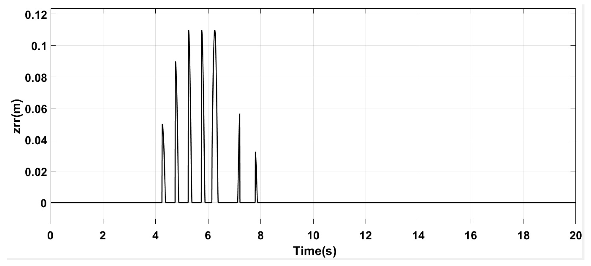
3.3.1. Case 1: Positive Road Disturbances

For convenience of analysis, positive road disturbances are considered in this case; therefore, the most common type of road disturbances used for analysis is of the form:
Y = A cos ( ω t + θ )
where range of time is taken from 0 to 30 s Front road disturbance is shown in Figure 4.
The rear road disturbance graph shown in Figure 5 is designed by giving a typical delay (used for analysis purposes) of 4.25 s to the graph of front road disturbance as first the disturbance is faced by front tyres and then by the rear tyres.

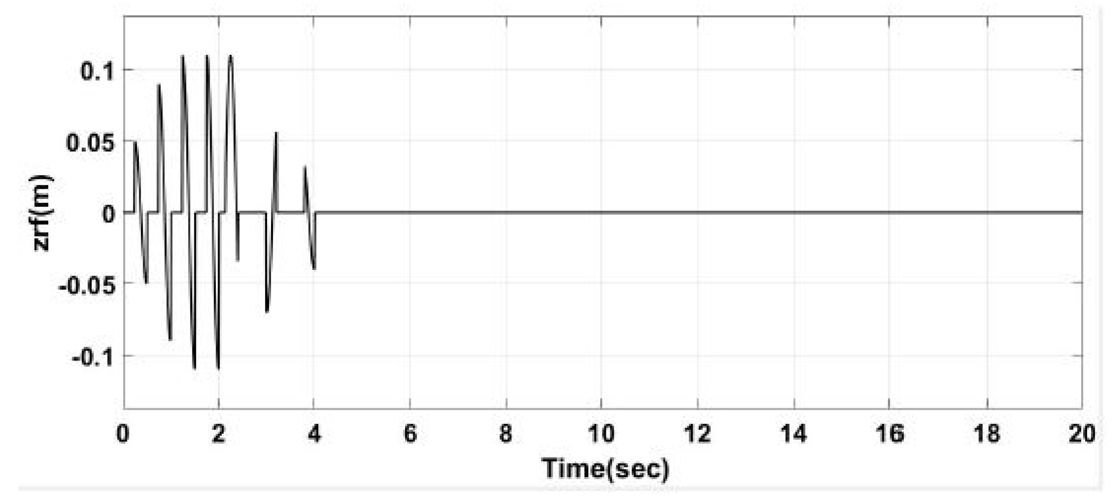
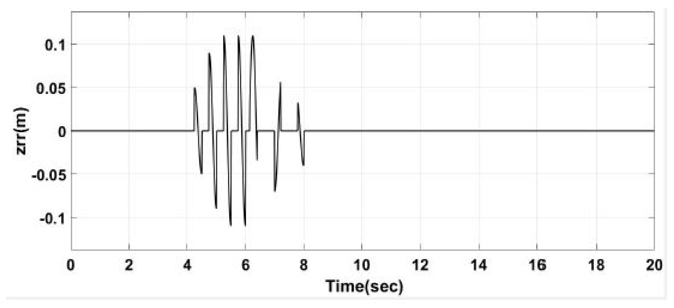
3.3.2. Case 2: Positive and Negative Road Disturbances

For practical purposes, both positive and negative road disturbances are taken into account as shown in Figure 6 and Figure 7 for both front and rear side respectively and then applied to the designed system. The Matlab function remains the same for both the cases except a product of 1 in the later case.
In Simulink, for designing the control law, R, E, I and H Blocks are coupled to the multiplexer in as per equations of control law u while K will be designed according to LQR Controller. Gain block is connected to demultiplexer as there are two outputs which will be the inputs of the those respective blocks of forced inputs u 1 and u 1 . The forced inputs will then eventually linearize the system. Finally, connecting all the blocks to a main block of Half-Car model as its inputs which actually contains all state equations of the system. The outputs of the main block are the actual variables to be controlled. The outputs of Road Disturbance sub-system and control law are now the inputs of the main block. The Simulink block diagram is shown in Figure 8. For simulation, typical half car model parameters are used.

4. Results and Discussions

When the whole system is coupled and simulated, the results for both the cases are shown in Figure 9, Figure 10, Figure 11, Figure 12, Figure 13 and Figure 14 for Case 1 and Figure 15, Figure 16, Figure 17, Figure 18, Figure 19 and Figure 20.

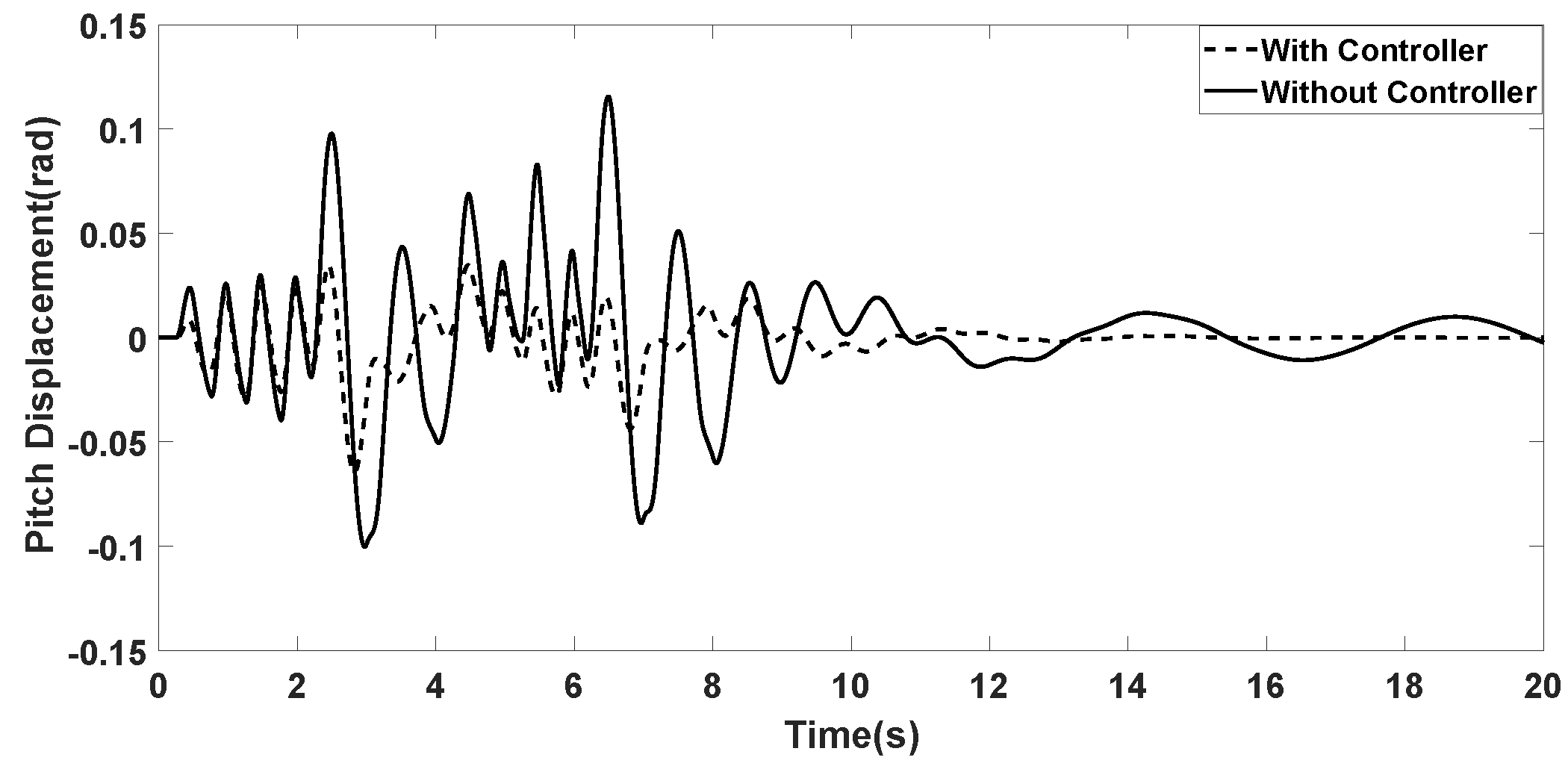
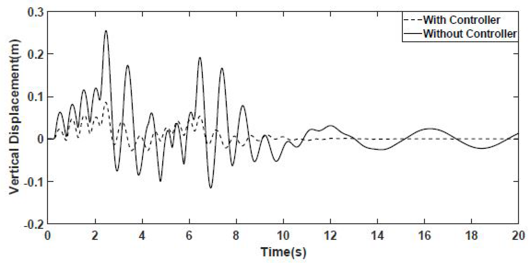
4.1. Results of Case 1: Positive Road Disturbances

In the graph of vertical displacement shown in Figure 9, the peak of vertical displacement has gone to 0.23 m but now, the peak has reduced to 0.08 m while on the other side the negative peak without controller is 0.15 m has reduced to nearly 0.04 m by using controller.
In the graph of pitch displacement shown in Figure 10, the peak of pitch displacement has gone to 0.125 m but now, the peak has reduced to 0.03 m while on the other side the negative peak without controller is 0.1 m has reduced to nearly 0.052 m by using controller. After the bumps, by using controller it came back to its steady state value 0 m while without using controller it took a time to reach its steady state value.
As vertical displacement and pitch displacement are our system outputs so, these both are very vital in this sense.
In the graph of vertical acceleration shown in Figure 11, the peak of vertical acceleration has gone to 18 but now, the peak has reduced to 8, similarly there are several other peaks so its better to see RMS value in this case which is given in Table 2.
In the graph of pitch acceleration shown in Figure 12, the peak of pitch acceleration has gone to 11 but now, the peak has reduced to 6, similarly there are several other peaks so its better to see RMS value in this case which is given in Table 2.
In the graph of front suspension travel shown in Figure 13, the peak of front suspension travel has gone to 0.014 but now, the peak has reduced to 0.02 while on the other side it is not 0 in rear suspension travel region but using controller it has reduced to almost 0 in that region.
In the graph of rear suspension travel shown in Figure 14, the peak of rear suspension travel has gone to 0.15 but now, the peak has reduced to 0.03 while on the other side it is not 0 in front suspension travel region but using this technique it has reduced to almost 0 in that region.

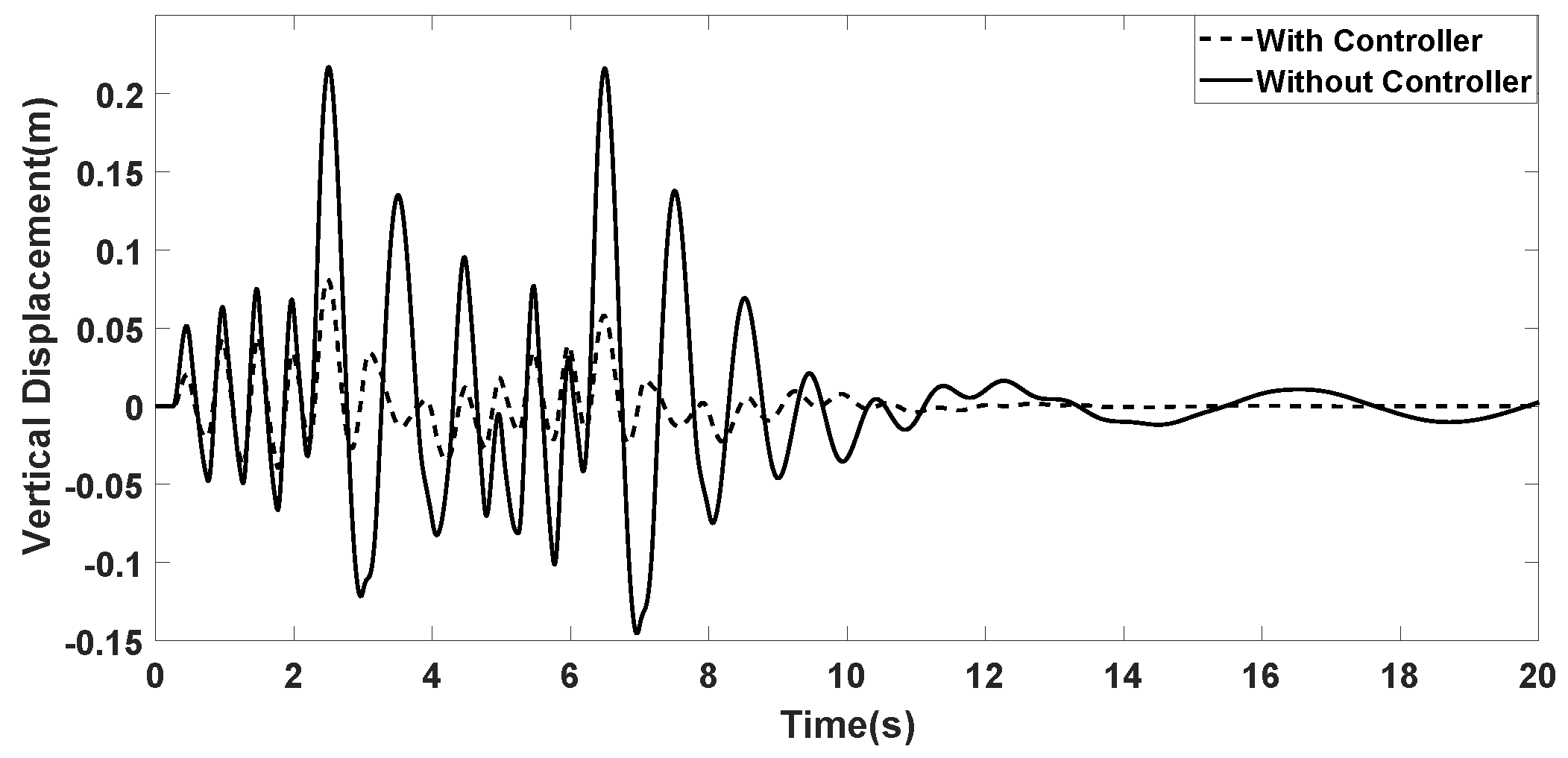
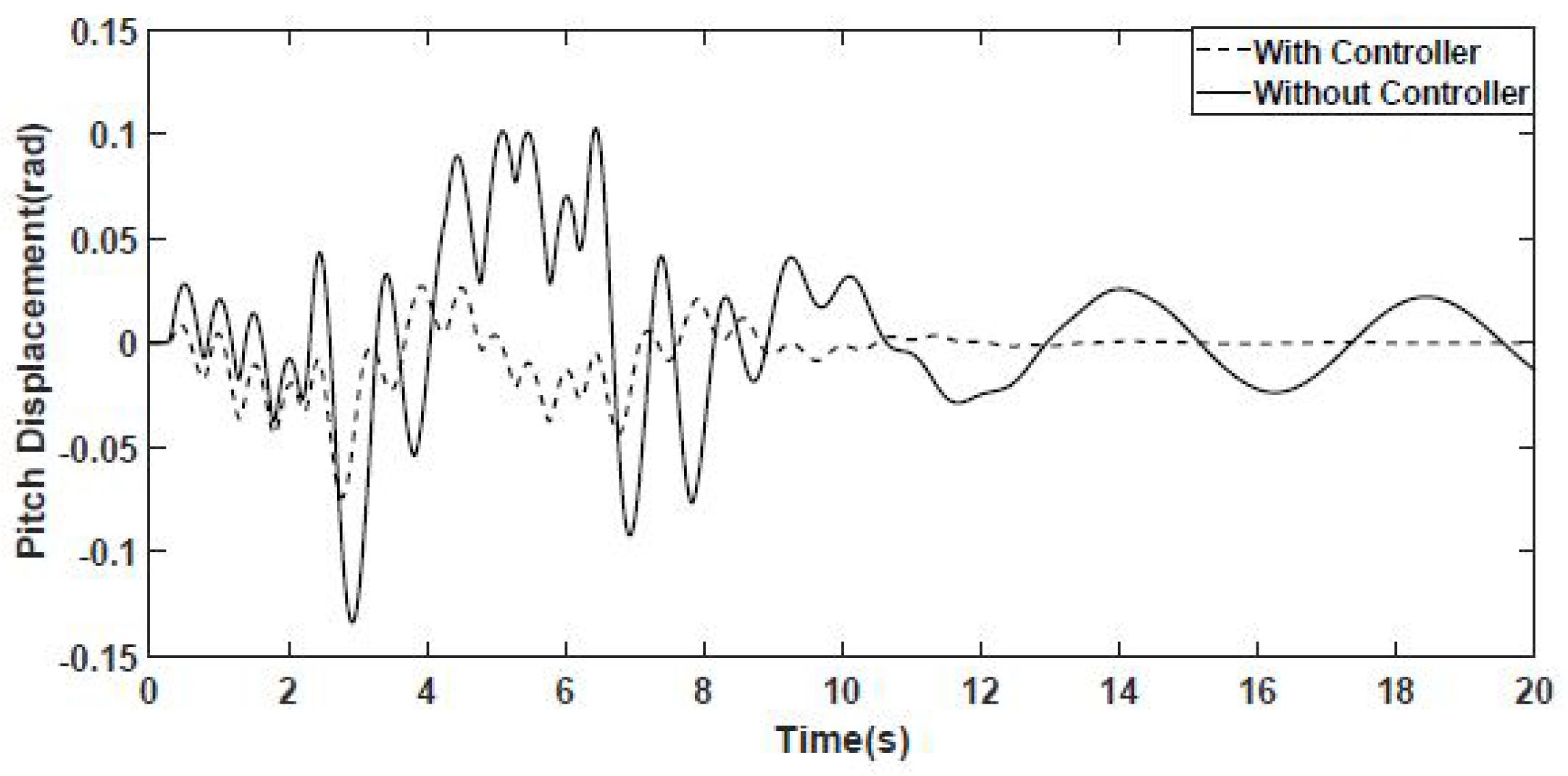
4.2. Results of Case 2: Positive and Negative Road Disturbances

In the graph of vertical displacement PN shown in Figure 15, the peak of vertical displacement has gone to 0.26 m but now, the peak has reduced to 0.08 m while on the other side the negative peak without controller is 0.13 m has reduced to nearly 0.02 m by using the controller.
In the graph of pitch displacement shown in Figure 16, the peak of pitch displacement has gone to 0.125 m but now, the peak has reduced to 0 m while on the other side the negative peak without controller is 0.14 m has reduced to nearly 0.07 m by using control law and the controller.
In the graph of vertical acceleration shown in Figure 17, the peak of vertical acceleration has gone to 16 but now, the peak has reduced to 5, similarly there are several other peaks so its better to see RMS value in this case which is given in Table 3.
In the graph of pitch acceleration shown in Figure 18, the peak of pitch acceleration has gone to 8.5 but now, the peak has reduced to 3.
In the graph of front suspension travel shown in Figure 19, the peak of front suspension travel has gone to 0.0125 but now, the peak has reduced to 0.03 while on the negative side it has reached to 0.15 but now it has reduced to almost 0.03 .
In the graph of rear suspension travel shown in Figure 20, the peak of rear suspension travel has gone to 0.15 but now, the peak has reduced to 0.03 and same reduction level on the other side.
Effect of road disturbances is reduced up to great extent in all the states. The results obtained in RMS values for Case 1 are compared with the previous techniques are given in Table 2. The values obtained from figures of Case 2 are given in Table 3 in which the values of states are compared without controller and with controller are given and the improvement is given in percentage. This technique has demonstrated the results which proved it to be the most economical solution for stabilizing and implementing this nonlinear system in the real world. This technique is cost effective as compared to other techniques i.e., road adaptive algorithm, PID and many others. Comparative analysis with the work [8,10] shows that states are much more stable in comparison to several previous techniques and the RMS values of the given states are much more reduced than as obtained in the above stated work.The simulation results exhibited that the half-car model considering road input conditions presented in [17] was found to have a maximum accuracy of 65% while the design proposed in this paper proves to have a maximum accuracy of 85% of which is significantly higher.

5. Conclusions

Effective road handling and better ride quality are two conflicting requirements in design of a suspension system. In active suspension system, additional design freedom is provided by the active element (linear actuator) present therein. In this paper, the objective of minimizing the road disturbances of a half-car model is achieved successfully using the Feedback Linearization technique and LQR controller. A nonlinear transformation is defined which transforms the nonlinear model of the active suspension system into normal form, which is then linearized using a nonlinear control law. Linearizing the nonlinear system and then applying an LQR greatly reduced the complexity of implementation in Simulink/Matlab as well as in real time. The technique proposed in this research solved the problem a great extent by maintaining a trade-off between the good quality ride and road handling performance by not letting the suspension travels to rise so much in presence of road disturbances. Simulation results of case 1 and case 2 presented in this paper revealed that compared with other techniques, Feedback linearization technique applied along with LQR controller has a better response in reducing the amplitudes of states, overshoot and good dynamic performance.
In this work, it has been assumed that states of the system are measurable. As a future work, an LQG controller may be designed to achieve better ride quality when all the states are not measurable. Furthermore, driver dynamics can be added in the model of Half Car Active Suspension system to make the system more accurate.

Author Contributions

M.A. proposed the concept, M.A.K. and M.A. did formal analysis and designed methodology, M.A.K. performed mathematical model, M.A.K. performed simulations, M.A. and N.A. supervised the research work. M.A.K. wrote the original draft of paper and M.A. supervised it. H.P. did funding acquisition. A.W. provided resources and administered the manuscript submission process. A.W. and H.P. review and supervised the manuscript for final submission. All authors have read and agreed to the published version of the manuscript.

Acknowledgments

This research was supported by Basic Science Research Program through the National Research Foundation of Korea (NRF) funded by the Ministry of Education (2017R1D1A3B03035693).

Conflicts of Interest

The authors declare no conflict of interest.

References

  1. Karnopp, D. Theoretical Limitations in Active Vehicle Suspensions. Veh. Syst. Dyn. 1986, 15, 41–54. [Google Scholar] [CrossRef]
  2. Yue, C.; Butsuen, T.; Hedrick, J.K. Alternative Control Laws for Automotive Active Suspensions. J. Dyn. Syst. Meas. Control. 1989, 111, 286–291. [Google Scholar] [CrossRef]
  3. Hrovat, D. Optimal Active Suspension Structures for Quarter-Car Vehicle Models. Automatica 1990, 26, 845–860. [Google Scholar] [CrossRef]
  4. Hrovat, D. Applications of Optimal Control to Advanced Automotive Suspension Design. J. Dyn. Syst. Meas. Control. 1993, 115, 328–342. [Google Scholar] [CrossRef]
  5. KrstiC, M.; Kokotovic, P.V. Adaptive Nonlinear Design with Controller-Identifier Separation and Swapping. IEEE Trans. Autom. Control. 1995, 40, 426–440. [Google Scholar] [CrossRef] [Green Version]
  6. Cho, B.K.; Ryu, G.; Song, S.J. Control Strategy of An Active Suspension for a Half Car Model with Preview Information. Int. J. Automot. Technol. 2005, 6, 243–249. [Google Scholar]
  7. Chander, B. Modelling and Analysis of Half Car Vehicle Suspension System Using Fuzzy Logic Controller. Bachelor’s Thesis, Mechancial Engineering Department, Sri Venkateshwara Univeristy College of Engineering, Tirupati, India, 2009. [Google Scholar]
  8. Huang, C.J.; Lin, J.S.; Chen, C.C. Road-Adaptive Algorithm Design of Half-Car Active Suspension System. Expert Syst. Appl. 2010, 37, 4392–4402. [Google Scholar] [CrossRef]
  9. Li, H.; Liu, H.; Hand, S.; Hilton, C. A Study on Half-Vehicle Active Suspension Control using Sampled-Data Control. In Proceedings of the Chinese Conference on Control and Decision, Mianyang, China, 23–25 May 2011; pp. 2635–2640. [Google Scholar]
  10. Alexandru, C.; Alexandru, P. Dynamic Analysis of a Half-Car Model with Active Suspension. In Proceedings of the 2nd International Conference on Circuits, Systems, Control and Signals, Prague, Czech Republic, 26–28 September 2011; pp. 36–41. [Google Scholar]
  11. Karuppaiah, N.; Sujatha, C.; Ramamurti, V. Modal vibration/stress analysis of a passenger vehicle by FEM. In Proceedings of the Symposium on International Automotive Technology, Nantes, France, 2–4 July 2012. [Google Scholar]
  12. Souilem, H.; Mehjoub, S.; Derbel, N. Intelligent Control for a Half-Car Active Suspension by Self-Tunable Fuzzy Inference System. Int. J. Fuzzy Syst. Adv. Appl. 2015, 2, 9–15. [Google Scholar]
  13. Ata, A.B.; Kunya, A.A. Half Car Suspension System Integrated With PID Controller. In Proceedings of the 29th European Conference on Modelling and Simulation, ECMS, Albena (Varna), Bulgaria, 26–29 May 2015. [Google Scholar]
  14. Turakhia, T.; Modi, M. Mathematical Modelling and Simulation of a Simple Half—Car Vibration Model. Int. J. Sci. Res. Dev. 2016, 4, 2321. [Google Scholar]
  15. Rizvi, S.M.H.; Abid, M.; Khan, A.Q.; Satti, S.G.; Latif, J. H control of 8 degrees of freedom vehicle active suspension system. J. King Saud-Univ. Eng. Sci. 2016, 30, 161–169. [Google Scholar] [CrossRef] [Green Version]
  16. Kadam, R.N.; Gangavane, S.A.; Shaikh, S.M.; Manjarekar, S.S.; Bamankar, P.B. Vibrational Analysis of Half Car Model. J. Int. Eng. Res. (IERJ) 2017, 1, 69–72. [Google Scholar]
  17. Wang, Z.-F.; Dong, M.-M.; Gu, L.; Rath, J.-J.; Qin, Y.-C.; Bai, B. Influence of Road Excitation and Steering Wheel Input on Vehicle System Dynamic Responses. Appl. Sci. 2017, 7, 570. [Google Scholar] [CrossRef] [Green Version]
  18. Shelke, G.D.; Mitra, A.C. Analysis and Validation of Linear Half Car Passive Suspension System with Different Road Profiles. In Proceedings of the 7th National Conference on Recent Developments in Mechanical Engineering RDME-2018, Ghent, Belgium, 9–10 July 2018; pp. 14–19. [Google Scholar]
  19. Nassar, A.; Al-Ghanim, A. Modeling, Simulation, and Control of Half Car Suspension System Using Matlab/Simulink. Int. J. Sci. Res. (IJSR) 2018, 7, 351–362. [Google Scholar]
  20. Hua, C.; Chen, J.; Li, Y.; Li, L. Adaptive prescribed performance control of half-car active suspension system with unknown dead-zone input. Mech. Syst. Signal Process. 2018, 111, 135–148. [Google Scholar] [CrossRef]
  21. Ghahremani, A.; Khaloozadeh, H.; Ghahremani, P. Adaptive sliding neural network-based vibration control of a nonlinear quarter car active suspension system with unknown dynamics. Vibroeng. Procedia 2018, 17, 67–72. [Google Scholar] [CrossRef] [Green Version]
  22. Gopala Rao, L.V.V.; Narayanan, S. Optimal response of half car vehicle model with sky-hook damper based on LQR control. Int. J. Dynam. Control 2019. [Google Scholar] [CrossRef]
  23. Sun, Z.Y.; Shao, Y.; Chen, C.C. Fast finite-time stability and its application in adaptive control of high-order nonlinear system. Automatica 2019, 106, 339–348. [Google Scholar] [CrossRef]
  24. Sun, Z.Y.; Zhang, D.; Meng, Q.; Chen, C.C. Feedback stabilization of time-delay nonlinear systems with continuous time-varying output function. Int. J. Syst. Sci. 2019, 50, 244–255. [Google Scholar] [CrossRef]
  25. Sun, Z.Y.; Dong, Y.Y.; Chen, C.C. Global fast finite-time partial state feedback stabilization of high-order nonlinear systems with dynamic uncertainties. Inf. Sci. 2019, 484, 219–236. [Google Scholar] [CrossRef]
  26. Hamdoon, F.O.; Faisal, B.M. Simulation of Active Suspension System for Half Vehicle Model under Different Road Profile. Univ. Thi-Qar J. Eng. Sci. 2019, 10, 13–17. [Google Scholar] [CrossRef]
  27. Rathai, K.M.M.; Sename, O.; Alamir, M. GPU-Based Parameterized NMPC Scheme for Control of Half Car Vehicle With Semi-Active Suspension System. IEEE Control. Syst. Lett. 2019, 3, 631–636. [Google Scholar] [CrossRef]
  28. Kanchwala, H. Vehicle Suspension Model Development using Test Track Measurements. Proc. Inst. Mech. Eng. Part J. Automob. Eng. 2020, 234, 1442–1459. [Google Scholar] [CrossRef]
  29. Isidori, A. Nonlinear Control Systems, 3rd ed.; Springer: London, UK, 1995; pp. 219–291. [Google Scholar]
Figure 1. Flowchart of Research.
Applsci 10 03075 g001
Figure 2. Half car model of ASS [8].
Applsci 10 03075 g002
Figure 3. Nonlinear System of Half Car ASS.
Applsci 10 03075 g003
Figure 4. Front Road Disturbance.
Applsci 10 03075 g004
Figure 5. Rear Road Disturbance.
Applsci 10 03075 g005
Figure 6. Front Road Disturbance PN.
Applsci 10 03075 g006
Figure 7. Rear Road Disturbance PN.
Applsci 10 03075 g007
Figure 8. Simulink model.
Applsci 10 03075 g008
Figure 9. Vertical Displacement.
Applsci 10 03075 g009
Figure 10. Pitch Displacement.
Applsci 10 03075 g010
Figure 11. Vertical Acceleration.
Applsci 10 03075 g011
Figure 12. Pitch Acceleration.
Applsci 10 03075 g012
Figure 13. Front Body Displacement.
Applsci 10 03075 g013
Figure 14. Rear Body Displacement.
Applsci 10 03075 g014
Figure 15. Vertical Displacement PN.
Applsci 10 03075 g015
Figure 16. Pitch Displacement.
Applsci 10 03075 g016
Figure 17. Vertical Acceleration.
Applsci 10 03075 g017
Figure 18. Pitch Acceleration.
Applsci 10 03075 g018
Figure 19. Front Body Displacement.
Applsci 10 03075 g019
Figure 20. Rear Body Displacement.
Applsci 10 03075 g020
Table 1. State Variables and Description.
StatesState VariablesVariable Names
x 1 zVertical Displacement
x 2 z ˙ Vertical Velocity
x 3 θ Angular Displacement
x 4 θ ˙ Angular Velocity
x 5 z s f z u f Front Suspension Travel
x 6 z ˙ u f Velocity of Front Unsprung Mass
x 7 z s r z u r Rear Wheel Suspension Travel
x 8 z ˙ u r Velocity of Rear Unsprung Mass
Table 2. RMS values comparison with previous techniques.
StatesValues (m)Research PapersReduction in Amplitude (%)Reduced rms Values (%)
Vertical Displacement0.0180.024 [10]73.325 [10]
Vertical Acceleration1.32.5 [10]7648 [10]
Pitch Displacement0.0140.0273 [10]55.648 [10]
Pitch Acceleration0.831.8 [10]45.553.9 [10]
Front Suspension Travel0.0110.022 [8]85.750 [8]
Rear Suspension Travel0.0120.020 [8]8040 [8]
Table 3. RMS values comparison with previous techniques.
StatesWithout Controller (m)With Controller (m)Improvement (%)
Vertical Displacement0.050.01668
Vertical Acceleration4.41.370.4
Pitch Displacement0.030.0166.7
Pitch Acceleration2.30.6970
Front Suspension Travel0.0220.01341
Rear Suspension Travel0.0250.01636

