Bentonite Extrusion into Near-Borehole Fracture

Abstract

In this paper, we discuss laboratory experiments of bentonite swelling and coupled finite element simulations to explicate bentonite extrusion. For the experiments, we developed a swell cell apparatus to understand the bentonite migration to the near-borehole fracture. We constructed the swell cell using acrylic, which comprised of a borehole and open fracture. Initially, the borehole of the swell cell was filled with bentonite and liquid. Then, the apparatus was sealed for observations. Due to the liquid saturation increase of bentonite, its swelling pressure increased. The developed pressure caused the extrusion of bentonite into the fracture, and the flow of bentonite from the borehole decreased with time. Moreover, for the effectiveness of bentonite-based plugging, there is a limiting condition, which represents the relation between the maximum bentonite migration length with the fracture aperture. Additionally, we also performed the bentonite free swelling test to assess the swelling potential to the fluid salinity, and we observed that with the increase of the salinity, the swelling potential decreased. In addition, we present a fully coupled two-phases fluids flow (e.g., liquid and gas) and deformation flow finite element (FE) model for the bentonite column elements and swell cell model. We also combined the Modified Cam Clay (MCC) model and the swelling model for the bentonite deformation flow model. Then, we also present the validation of the bentonite model. To model other sub-domains, we used the poro-elastic model. Additionally, we obtained the transition between the wetting phase (i.e., liquid) and non-wetting phase (i.e., gas) using the Brooks–Corey model. From the finite element results, we observed that due to the liquid intrusion into the bentonite, the developed capillary pressure gradient results in a change of the hydro-mechanical behavior of the bentonite. Initially, we observed that due to the high capillary pressure gradient, the liquid saturation and the swelling pressure increased, which also decreased with time due to a reduction in the capillary pressure gradient. Thereby, the swelling pressure-induced bentonite migration to the fracture also decreased over time, and after the equilibrium state (for a negligible pressure gradient), there was no significant transport of bentonite into the fracture.

1. Introduction

The plugging of boreholes to achieve zonal isolation is imposed through regulations to avoid unwanted fluid migration and to protect the environment. This isolation is achieved using well-plugging materials, such as cement [1] or bentonite [2], with the selection of borehole plugging material depending on several conditions, including the well purpose, downhole reservoir conditions, and well lifecycle status (temporary plugging or permanent abandonment). Application of bentonite offers advantageous performance in some cases due to its high sorption, high swelling capacity, low permeability, low diffusivity, self-healing ability, and retention properties [3]. For the success of well plugging using bentonite, it is essential to ensure the integrity of the bentonite barrier and understand the ability of the bentonite to expand into and seal the void space that would otherwise serve as a pathway for unwanted fluid migration.

Beswick [4] reported that deep boreholes’ drilling depth ranged from 500 m to 12.2 km depending on geologic exploration and engineering applications (e.g., oil and gas industry, geothermal energy exploration and production, and deep disposal of hazardous and radioactive waste). In the USA alone, there are known to be millions of existing deep boreholes, and Brady et al. [5] reported that approximately 40,000 new deep boreholes are drilled each year. Additionally, from the available sources of data, Townsend-Small et al. [6] reported that the number of onshore abandoned wells in the USA is approximately 2.3 million to 3.0 million. Townsend-Small et al. [6] also demonstrated the reasons behind the variation of the number of wells. Dilmore et al. [7] also showed that the estimated number of drilled wells in Pennsylvania only approximately ranged from 300,000 to 500,000. Moreover, from the Pennsylvania Department of Environmental Protection (PADEP) statistics, Mitchell and Casman [8] presented that the average cost to plug a 914-m well (shallow deep boreholes, see also Beswick [4]) is approximately $60,000, while the reclamation cost is about $100,000. Also, from the Cabot Oil and Gas Corporation data, Mitchell and Casman [8] demonstrated that the plugging and abandonment cost of the Marcellus Shale gas in Pennsylvania is approximately $700,000 per well. Costs to properly plug and abandon deep boreholes can be expected to be billions of dollars, and research to ensure the effectiveness of borehole sealing is warranted.

Over the last few decades, several researchers have performed experiments (e.g., Kanno and Wakamatsu [9]; Tanai and Matsumoto [10]), analytical solutions (e.g., Bolchover et al. [11]; Svoboda [12]), and numerical simulations (e.g., Kanno et al. [13]; Borrelli and Ahn [14]) to investigate the physical processes of bentonite barrier development and performance for the sealing of boreholes as well as near-borehole fracture. Even though in the abovementioned references the study domains’ geometry is different, those studies provided a basic understanding of essential phenomena contributing to the model system behavior. Also, those studies explain the mechanisms of bentonite migration. However, in the above cases, the plasticity of bentonite for multiphase media is ignored (see also Sanchez et al. [15]). Besides, it is noteworthy that there are very few attempts where coupled fluids and deformation flow through a near-borehole fracture were presented for a heterogeneous media, which is the motivation of this paper. Additionally, among others, Helmig [16] demonstrated the numerical complexities of fluid flow through heterogeneous media (see Kueper and Frind [17] experiments). For the two-phases fluids flow through porous media, the selection of fluids’ phase primary variables is crucial (see also Aziz and Settari [18]; Helmig [16]). For similar fluid flow cases in homogeneous media, the effect of fluids’ phases primary variables is negligible (see Park et al. [19]). Finite element (FE) modeling can address coupled deformation and fluids flow through near-borehole fractures. This modeling approach offers a means to capture the relevant complexity of the system and develop new insights into critical behavior. This is the motivation for the finite element modeling study described herein.

Additionally, Shad et al. [20] presented several methods to simulate fluid flow through fractured media, including two-phases flow, considering Darcy’s equation, miscible flow of two fluids, pipe flow model, and flow through parallel plates. Snow [21] and Witherspoon et al. [22] reported that fluid flow through a fracture bounded by two plates supports Darcy’s analogous equation, if (i) the intrinsic permeability $\left(\mathit{k}\right)$ is expressed as the cube of the hydraulic aperture divided by 12, (ii) the aperture (b) is uniform and temporally constant, (iii) fluid flow is assumed as laminar, and (iv) there are initially no materials in the fracture. Herein, we used the first approach to model flow behavior through the fracture.

In this study, we summarize results from a bentonite free swelling test and a bentonite swell cell experiment, and also present finite element (FE) modeling motivated by those experiments to explore the dynamics of bentonite swelling, fluids flow, and stress response.

2. Materials and Methods

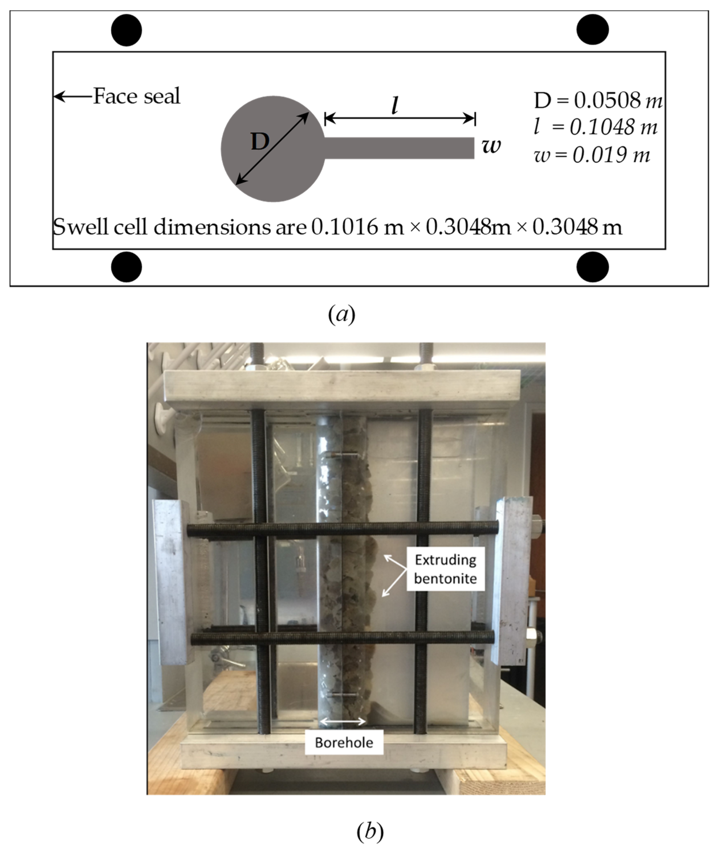
2.1. Experimental Setup

At ambient temperature and pressure, we allowed unconfined bentonite samples to swell freely in beakers when exposed to aqueous brines of a given salinity. We performed a total of six tests, varying salinity (g/L) across the following values: 0, 5, 7.5, 10, 15, and 20, where the value zero represents distilled water. After 24 h, we observed that the change of the swelled bentonite volume due to liquid intrusion was negligible, and we considered this state as the swelling equilibrium state. Then, we calculated the swelling potential as $s_p = \frac{\partial h}{h} = \frac{\partial V}{V_0}$, where $h$ and $\partial h$ are the height of the bentonite in the beaker before swelling and after swelling, respectively, while $V_0$ and $\partial V$ are the initial volume and change of volume (see Figure 1). The value of $s_p$ of an unconfined medium represents an indicator of the developed swelling pressure of the same medium under confining conditions [23].

Additionally, we developed a laboratory-scale swell cell apparatus, as illustrated in Figure 2. We performed swell cell experiments to understand bentonite’s migration behavior in the near-borehole fracture due to the expanded swelling pressure. We used transparent acrylic (poly (methyl methacrylate), PMMA) to ensure the bentonite extrusion could be observed in the swell cell. The exterior dimensions of the swell cell were 0.1016 m × 0.3048 m × 0.3048 m. A cylindrical chamber (diameter and height of 0.0508 and 0.3048 m, respectively) represented the boreholes. A slot (see Figure 2a) with a crack length $\left(l\right) \mathrm{of} 0.1048 \mathrm{m}$ and crack width $\left(w\right) \mathrm{of} 0.0109 \mathrm{m}$ was also included, which simulated the near-borehole crack.

To perform the swell cell test, we filled the borehole chamber with commercially available CETCO Puregold medium-coarse natural sodium bentonite pellets (0.0064 to 0.0095 m in size) and liquid. The bentonite was composed of Smectite group minerals, calcium carbonate, quartz, and cristobalite. Its density was 1109.28 kg/m³, while its pH in aqueous solution ranged between 8.5 to 11. We sealed the apparatus so that the incremental swelling pressure would not cause the apparatus to open or otherwise fail. We observed the swell cell over time to gain insight into how bentonite migrated into the near-borehole crack (see Figure 2b, bottom). Results from this experiment were qualitative in nature. While they did not provide parameter values to be used directly in the numerical model, nonetheless, they provided motivation for the geometry and conditions used in the modeled system.

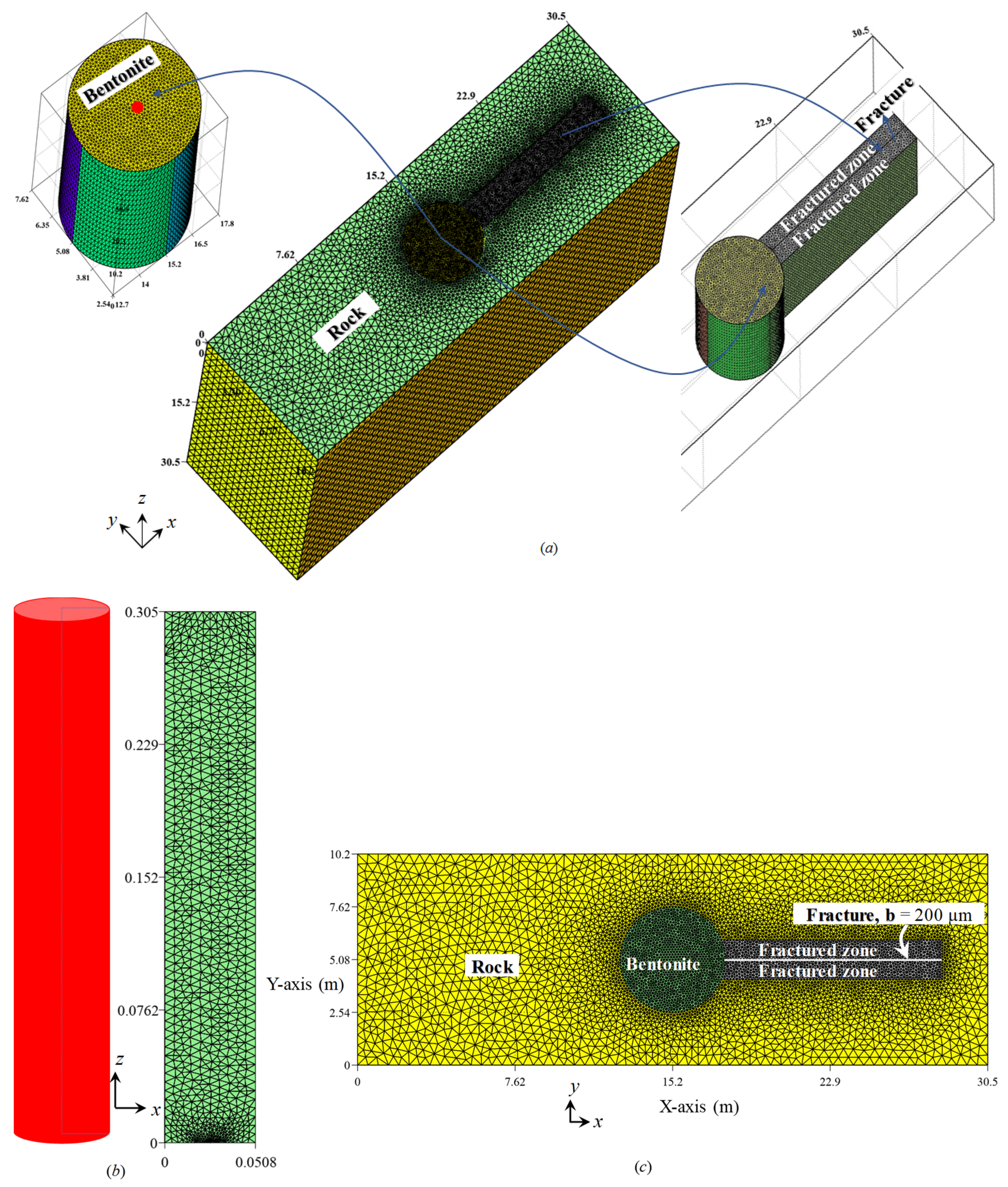
2.2. Numerical Modeling

For the FE solutions, mesh generation, and post-processing, we used open source code, OpenGeoSys [25], Gmsh [26], and VisIt [27], respectively. In FE solutions, two-phases flow is coupled with deformation flow. For the two-phases flow, we treated water and air as the wetting phase fluid and the non-wetting phase fluid, respectively. We also considered two primary variables for the two-phases flow: The capillary pressure and the gas pressure. Additionally, points of interests for the deformation flow were the displacement and stress variables. It is noteworthy that due to the unavailability of the testing facility to obtain the swell cell model data for the heterogeneous domains, we used model parameters from the published literature. Additionally, to make the model parameters coherent with the geometry domain, we also extended the swell cell geometry. In Figure 3, we illustrate details of the geometric sections that were used for the numerical simulations. In this paper, we present two types simulations. They are (i) bentonite column simulation (see Figure 3b) and (ii) swell cell equivalent simulation (see Figure 3c). In the homogeneous three-phases medium, to understand the bentonite swelling phenomena, we considered a small section of the borehole cylindrical bentonite sample, which is the motivation of the first case numerical simulation (see also Figure 3b). Additionally, to explore the similar swelling phenomena in the heterogeneous three-phases mediums and associated numerical complexities in the coupled finite element solutions, we considered a cross-section of the swell cell along the x-y plane (see Figure 2 and Figure 3c). The swell cell geometry comprised of a cylindrical hole representing the borehole, a rectangular block of acrylic illustrating the rock, and acrylic inserts that were used to control the fracture width, representing the fractured zones and fracture. Except for the fracture, to mesh all sub-domains in the swell cell, we used triangular elements, while for the fracture sub-domain, we used 1D line elements with constant aperture (b = 200 µm). It is noteworthy that dynamic fracture propagation is beyond the scope of this paper. Additionally, we also ignored the failure state and assumed that the medium was in a static equilibrium condition. For the bentonite model, we coupled the MCC model (Roscoe and Burland [28]), the swelling model (Rutqvist [29]), and two-phases fluids model. For all other sub-domains, we coupled the poro-elastic model (see Coussy [30]) with the two-phases fluids flow model.

Additionally, in the FE solutions, for each phase (solid, liquid, and gas), we also considered different shape functions (see Zienkiewicz et al. [31]). For the FE domain discretization, the importance of different shape functions for each phase depending on the discretized element shape (e.g., triangular) is emphasized in many multiphase flow FE modeling textbooks (see Lewis and Schrefler [32]; Ehlers and Bluhm [33]). For the sake of completeness, it should be noted that if the degree of freedom (DOF) for the deformation field (e.g., displacement, stress, strain) is inconsistent with the DOF for the fluids flow (e.g., gas and liquid), there is an accuracy as well as convergence issue for heterogeneous mediums (see Potts and Zdravkovic [34]; Zienkiewicz et al. [29]). Moreover, in the literature, for FE simulations, there are several coupling mechanisms to couple two-phases fluids and deformation flow, for example, monolithic coupling and sequential coupling (see Kolditz et al. [35]). It is noteworthy that without mass lumping and upwinding techniques (see Helmig [16]), achieving convergence in sequential coupling for heterogeneous mediums is challenging and in most cases impossible. Therefore, in this paper, for the coupling, we used monolithic coupling. Additionally, for the solutions of the linear and non-linear equations, we used the SpBICSGSTAB solver (see Chen et al. [36]) and the PICARD solver (see Paniconi and Putti [37]), respectively.

Moreover, we applied two-steps numerical simulation for bentonite migration into the near-borehole fracture. The first step involved the development of a representation of the wellbore excavation phase to arrive at the initial stress state, fluids pressure, and saturation after the completion of the excavation. Then, the excavation phase conditions were considered as the initial state in the mitigation phase, in which the bentonite was placed.

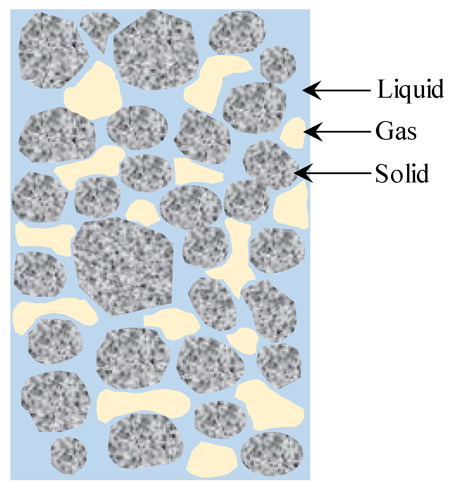
2.2.1. Governing Equations

We assumed that each domain consists of three phases: Solid, liquid, and gaseous phases (see Figure 4). We also assumed that (i) the medium is in the static equilibrium and the isothermal equilibrium, (ii) mediums support the small strain theory, (iii) interaction forces and dynamic actions or accelerations are negligible and ignored, (iv) fluid phases are immiscible, (v) microscopic solid particle are incompressible, (vi) phase component (e.g., vapor) and geochemical effects are ignored, (vii) solid phase is inert and isotropic, and (viii) fluids obey the Darcy’s law [38].

For the fluids phase, we considered as primary variables the capillary pressure, $p^c=p^g-p^l$, and the gas pressure ($p^g$), where $p^l$ stands for the liquid pressure. The governing equations for the two-phases flow in the deformable porous media included the momentum balance and mass balance equations, which are presented as follows (see also Bear and Bachmat [39]; Lewis and Schrefler [32]):

Momentum balance equation:

$$div \left[\acute{\mathit{\sigma }}-[p_g-S^l{p}_c\left]\mathit{I}\right]\right]+\left[\left(1-\phi \right){\rho }_R^s+\phi \left(1-S^l\right){\rho }_R^g+\phi S^l{\rho }_R^l\right]\mathit{g}=0.$$

(1)

Mass balance equation:

$$\phi {\rho }_R^l\frac{\partial S^l}{\partial p_c}\frac{\partial p_c}{\partial t}-div \left({\rho }_R^l\frac{k_{rel}^l\mathit{k}}{{\mu }^l}\left(\nabla p^g-\nabla p^c-{\rho }_R^l\mathit{g}\right)\right)+S^l{\rho }_R^{l}div\dot{\mathit{u}}=0.$$

(2)

$$-\phi {\rho }_R^g\frac{\partial S^l}{\partial p_c}\frac{\partial p_c}{\partial t}+\phi \left(1-S^l\right)\left(\frac{\partial {\rho }^g}{\partial p_g}\frac{\partial p_g}{\partial t}+\frac{\partial {\rho }^g}{\partial p_c}\frac{\partial p_c}{\partial t}\right)-div\left({\rho }_R^g\frac{k_{rel}^g\mathit{k}}{{\mu }^g}\left(\nabla p^g-{\rho }_R^g\mathit{g}\right)\right)+\left(1-S^l\right){\rho }_R^{g}div\dot{\mathit{u}}=0.$$

(3)

We made several constitutive assumptions in Equations (1)–(3), and corresponding models were applied within these governing equations to describe the system. Detailed derivation of the governing equations is presented in Appendix A. In Equations (1)–(3), ‘$div$’ is the divergence operator; $\mathit{I}$ is the identity tensor; $\mathit{g}$ is the gravitational acceleration acting only in the vertical direction; ${\rho }_R^s, {\rho }_R^g$, and ${\rho }_R^l$ are the reference density of the solid, gas, and liquid, respectively; $S^l = \frac{{\phi }^l}{\phi }$ and $S^g=\frac{{\phi }^g}{\phi }$ are the liquid saturation and gas saturation, respectively, which also holds $S^l + S^g = 1$; $\phi$, ${\phi }^l, \mathrm{and}$ ${\phi }^g$ are the medium porosity, liquid phase porosity, and gas phase porosity, respectively, which also supports $\phi = {\phi }^l + {\phi }^g$; $\acute{\mathit{\sigma }}$ is the effective Cauchy stress tensor (see also Terzaghi [40]); $\dot{\mathit{u}}$ is the velocity of solids; $\mathit{k}$ and $k_{rel}^j$ are the intrinsic permeability and relative permeability, respectively; ${\mu }^j$ is the viscosity of the fluid phase; and $j\in \left\{l,g\right\}$, l, and g stand for the liquid and gas, respectively.

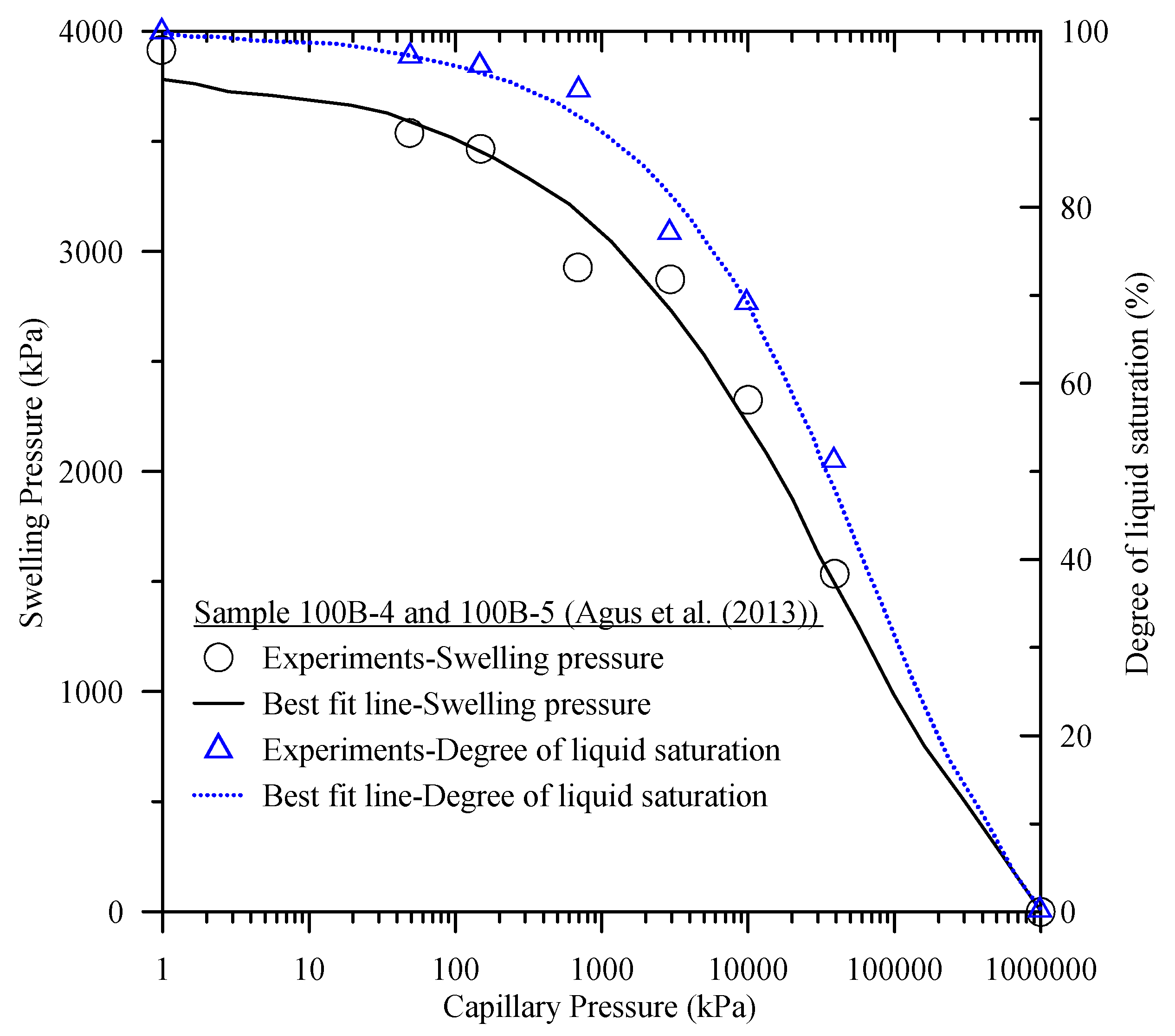
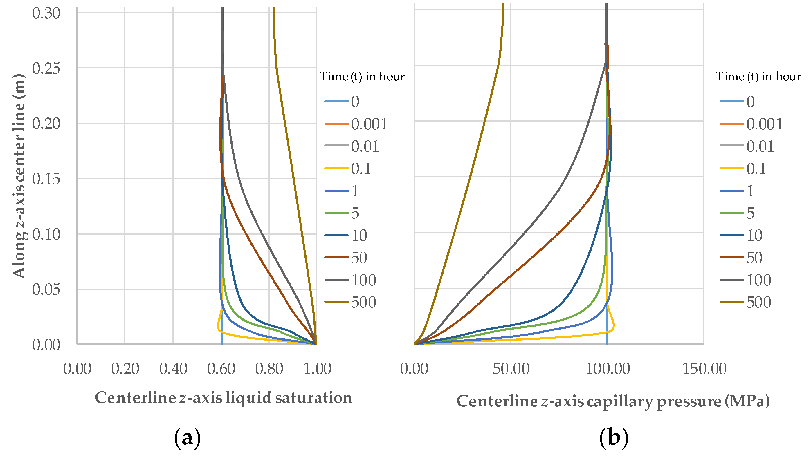
2.2.2. Capillary Pressure and Saturation Relations

In Equations (1)–(3), the capillary pressure and saturation relation can be obtained either from experiments (see also Fredlund and Rahardjo [41]) or by using curve fittings of empirical relations on the experimental results. For the latter case, there are many approaches, like the Brooks and Corey [42], model which is shown as follows:

$$S_e\left(p^c\right)=\frac{S^l-S^{rl}}{1-S^{rl}}={\left(\frac{p^c}{p^d}\right)}^{{\lambda }_{BC}} \mathrm{for} p^c\ge p^d,$$

(4)

where $S_e$, $S^l$, and $S^{rl}$ are the effective saturation, liquid saturation and residual liquid saturation; and $p^d$ and ${\lambda }_{BC}$ are Brooks and Corey’s [42] model parameters. Additionally,${\lambda }_{BC}$ is also known as the pore size distribution index while $p^d$ is known as the air entry pressure or the bubbling pressure (see also Bear and Bachmat [39]).

Again, in Equations (2) and (3), $k_{rel}^j$ is the relation of the liquid phase and gas phase with the effective saturation (see Equation (4)). For the Brooks–Corey model, such a relation was obtained using the Burdine theorem (see Burdine [43]) as follows:

$$k_{rel}^l={\left(S_e\right)}^{\frac{2+3{\lambda }_{BC}}{{\lambda }_{BC}}},$$

(5)

$$k_{rel}^g={\left(1-S_e\right)}^2\left(1-{\left(S_e\right)}^{\frac{2+{\lambda }_{BC}}{{\lambda }_{BC}}}\right).$$

(6)

It is worth to noting that Helmig [16] (see Chapter 2) discussed an empirical relation to transfer calibrated model parameters between the van Genuchten model parameters and the Brooks and Corey model parameters.

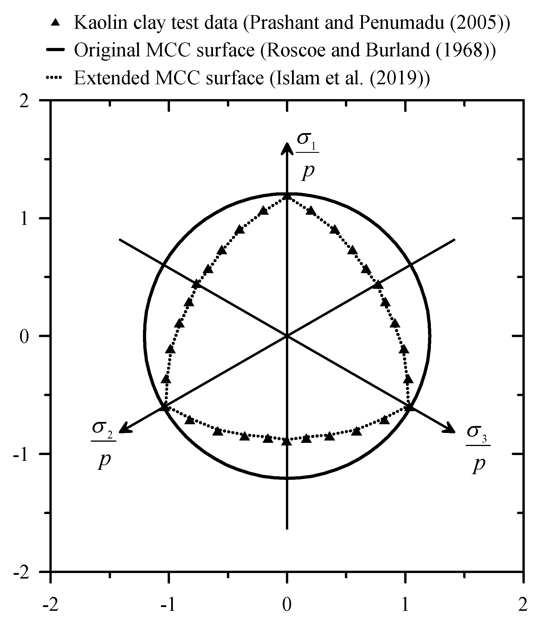
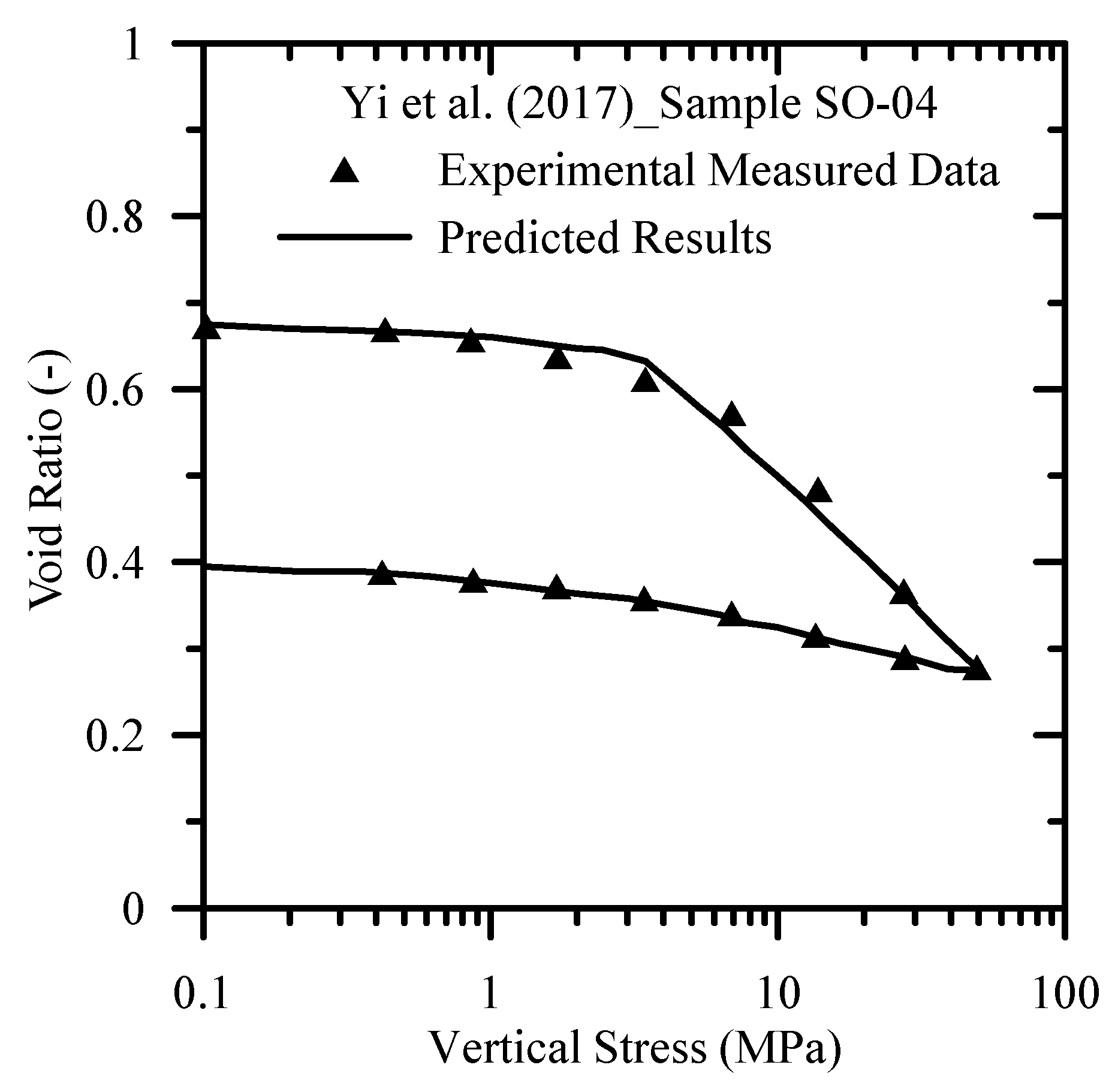
2.2.3. Constitutive Relations for Solid

To model the swell cell test scenario as detailed in the experimental methods section, we treated all solid phases as porous media through which two fluids phases (liquid and gas) flow. To model bentonite, we coupled two-phases flow, the Modified Cam Clay (MCC) model [28], and the bentonite swelling model proposed by Rutqvist [29]. For other media, two-phases flow was coupled with the linear poro-elastic model (see also Coussy [30]). For the poro-elastic medium, we assumed that the total strain has the elastic component only. In contrast, bentonite was assumed to exhibit incremental strain for elastic, swelling, and plastic strain. Thus:

$$d\mathit{\epsilon }=d{\mathit{\epsilon }}^e+d{\mathit{\epsilon }}^{sw}+d{\mathit{\epsilon }}^p,$$

(7)

where $d{\mathit{\epsilon }}^e$, $d{\mathit{\epsilon }}^{sw}$, and $d{\mathit{\epsilon }}^p$ are the elastic, swelling, and plastic strain, respectively.

For the small deformation and symmetry conditions, the strain–displacement relation can be written as:

$${\dot{\epsilon }}_{ij}=\frac{1}{2}\left(\frac{\partial {\dot{u}}_i}{\partial x_j}+\frac{\partial {\dot{u}}_j}{\partial x_i}\right),$$

(8)

where u is the displacement component.

Assuming (i) that isotropic material, (ii) small strain, and (iii) strain depends on the effective stress [40,44] and (iv) generalized Hooke’s law, we obtained the incremental elastic strain relation as follows (see Desai and Siriwardane [45]):

$$d{\mathsf{\sigma }}_{ij}^{\prime }=C_{ijkl}d{\epsilon }_{kl}^e,$$

(9)

where $d{\mathsf{\sigma }}_{ij}^{\prime }$ is the incremental effective stress and $C_{ijkl}$ is the fourth-order elastic stiffness tensor, which is also related to the fourth-order compliance tensor, $S_{ijkl}$:

$$C_{ijkl}=\frac{E}{2\left(1+\nu \right)}\left(\frac{2\nu }{1-2\nu }{\delta }_{ij}{\delta }_{kl}+{\delta }_{ik}{\delta }_{jl}+{\delta }_{il}{\delta }_{jk}\right),$$

(10)

where $E$ and $\nu$ are the elastic modulus and Poisson’s ratio, respectively; and $\delta$ is the Kronecker delta. Transferring $d{\mathit{\epsilon }}^e$ from Equation (7) to Equation (9), we can obtain:

$$\acute{\mathit{\sigma }}=\mathit{C} \left(d\mathit{\epsilon }-d{\mathit{\epsilon }}^{sw}- d{\mathit{\epsilon }}^p\right).$$

(11)

In Equation (11), Rutqvist [29] and Yi et al. [46] assumed $d{\mathit{\sigma }}^{sw}=-\mathit{C}d{\mathit{\epsilon }}^{sw}$ as the swelling-induced stress, in a confined space, which is a function of the maximum swelling pressure $\left({\mathit{\sigma }}_m^{sw}\right)$ and the liquid saturation $\left(S^l\right)$ as follows:

$$d{\mathit{\sigma }}^{sw}={\mathit{\sigma }}_m^{sw}d{S}^l\mathit{I},$$

(12)

where $\mathit{I}$ is the identity tensor, ${\mathit{\sigma }}_m^{sw}$ is the maximum swelling pressure, and $d{S}^l$ is the incremental liquid saturation.

The relationship between ${\mathit{\sigma }}_m^{sw}$ and $S^l$ for bentonite can be obtained from laboratory experiments. Additionally, in unsaturated soil mechanics, such types of experiments are also well known (see Fredlund and Rahardjo [41]). For the sake of completeness, typical experimental results (see Agus et al. [47]) are illustrated in Figure 5 to demonstrate the swelling pressure relation with the specific suction (also known as the matric suction or the capillary suction or the capillary pressure) and the degree of saturation. Additionally, from Figure 5, we observed that with the decrease of the suction, the degree of saturation and the swelling pressure also increase.

Additionally, the plastic component of the strain $\left(d{\epsilon }_{ij}^p\right)$ in Equations (7) and (11) can be written as [45]:

$$d{\epsilon }_{kl}^p=\mathsf{\Lambda }\frac{\partial f}{\partial {\acute{\sigma }}_{ij}}.$$

(13)

In Equation (13), $\mathsf{\Lambda }$ is the plastic multiplier, f represents the yield surface, f < 0 represents elastic behavior, f = 0 demonstrates that yielding is occurring, and f > 0 is not permissible (see Desai and Siriwardane [45]). Detailed derivation of Equation (13) can be found in many textbooks, and for the sake of completeness, we summarized it in Appendix B. In Equation (13), we revised the expression of the yield surface ($f$) in the original MCC model, and in Appendix B, we also present a comparison of the revised yield surface and the original MCC surface with the experimental results. More details about the importance of the extended MCC yield surface can be found in Islam et al. [48] and Islam and Gnanendran [49].

Additionally, a similar coupling of the MCC model with the Richards flow (see Richards [50]) is also applied in many field cases (e.g., SEALEX [46]; DECOVALEX [51]). It is noteworthy that in the two-phases fluids flow, assuming that the gas phase is immobile, the Richards flow is obtained. Also, the Richards flow application requires attention in field cases where both fluids are immiscible and mobile, e.g., CO₂ sequestration or a geothermal energy-type problem. In this regard, Wang et al. [52] demonstrated a comparison of the performance prediction in the Richards flow and two-phase fluid flow with experimental results.

Moreover, the original MCC model is formulated for two phases (liquid and solid) and is assumed as the fully liquid-saturated state (see also Roscoe and Burland [28]). In this paper, we considered the porous media as a three-phases system (solid, liquid, and gas, see Figure 4). To address the challenge of achieving convergence in a coupled three-phases system (see Park et al. [19]), we followed the monolithic coupling [35] of the fluids phases with the solid phase. Besides, we also introduced the mass lumping and upwinding techniques (Helmig [16]). It is noteworthy that from the evidence available in the literature of experimental results and analytical solutions, it is observed that for heterogeneous medium, when fluids pass the interface of dissimilar mediums, the selection of fluids’ phase primary variables is crucial (see also Helmig [16]; Park et al. [19]). Therefore, to avoid such a numerical instability in our heterogeneous composite domain of the swell cell’s equivalent finite element simulations, we considered the capillary pressure and gas pressure as the fluid phase’s primary variables.

Details of the coupled finite element solution are included in Appendix C of this manuscript.

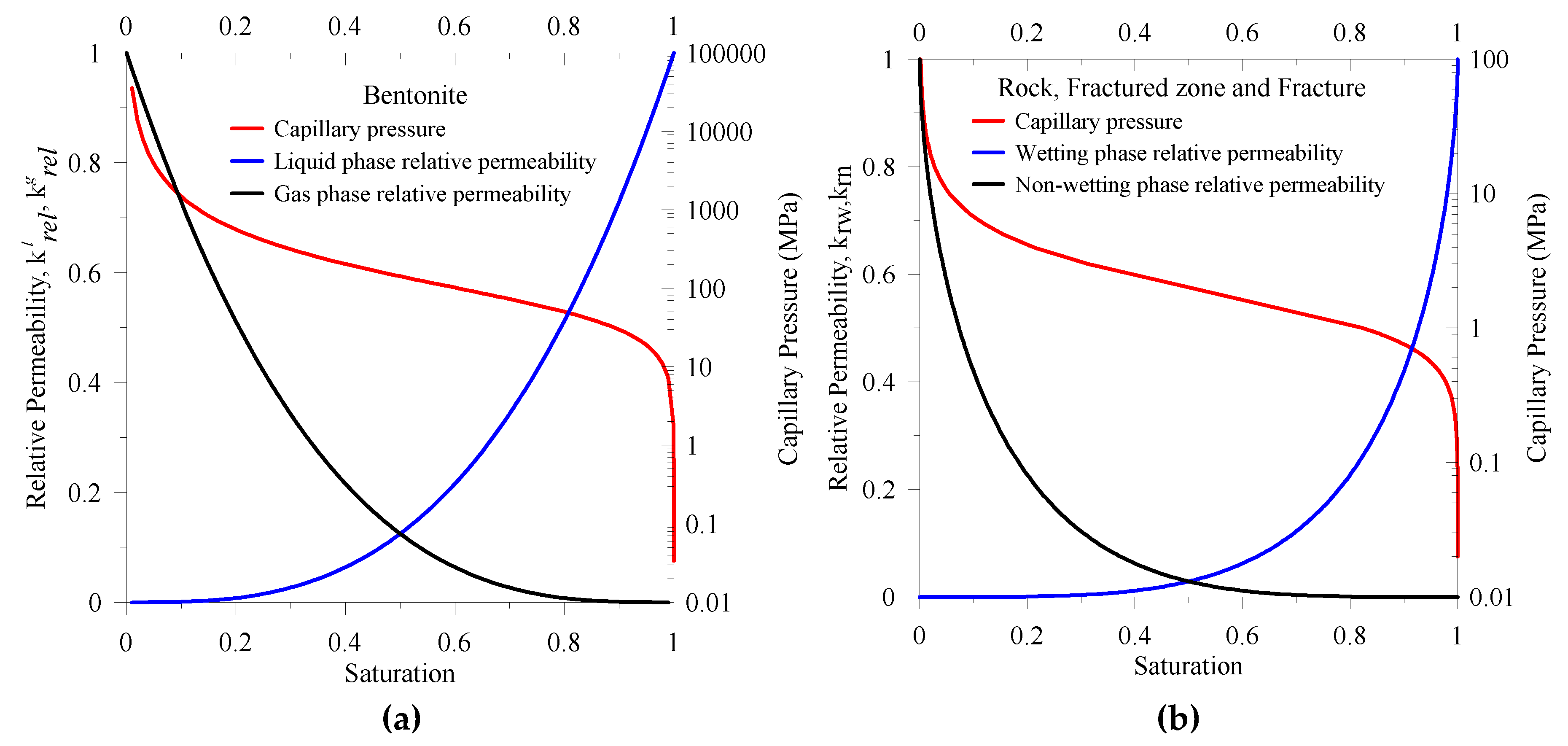
2.2.4. Constitutive Relations for Fluid Flow in the Fracture

Additionally, constitutive assumptions were used to facilitate the representation of the fluid flow in a near-borehole fracture. In this study, we assumed that fluids (liquid and gas) flow through a discrete fracture, which is bounded by two plates. For the finite element mesh generation of a fracture, we used 1D line elements with constant fracture aperture $\left(b\right).$ The intrinsic permeability $\left(\mathit{k}\right)$ in Equations (2) and (3) for the fracture is expressed, according to work by Yih [53] and Bear and Berkowitz [54], as:

$$k_f=\frac{b^2}{12}.$$

(14)

This equation has also been regularly used in experimental studies (e.g., Fourar and Bories [55]; Oron and Berkowitz [56]; Crandall et al. [57], among others).

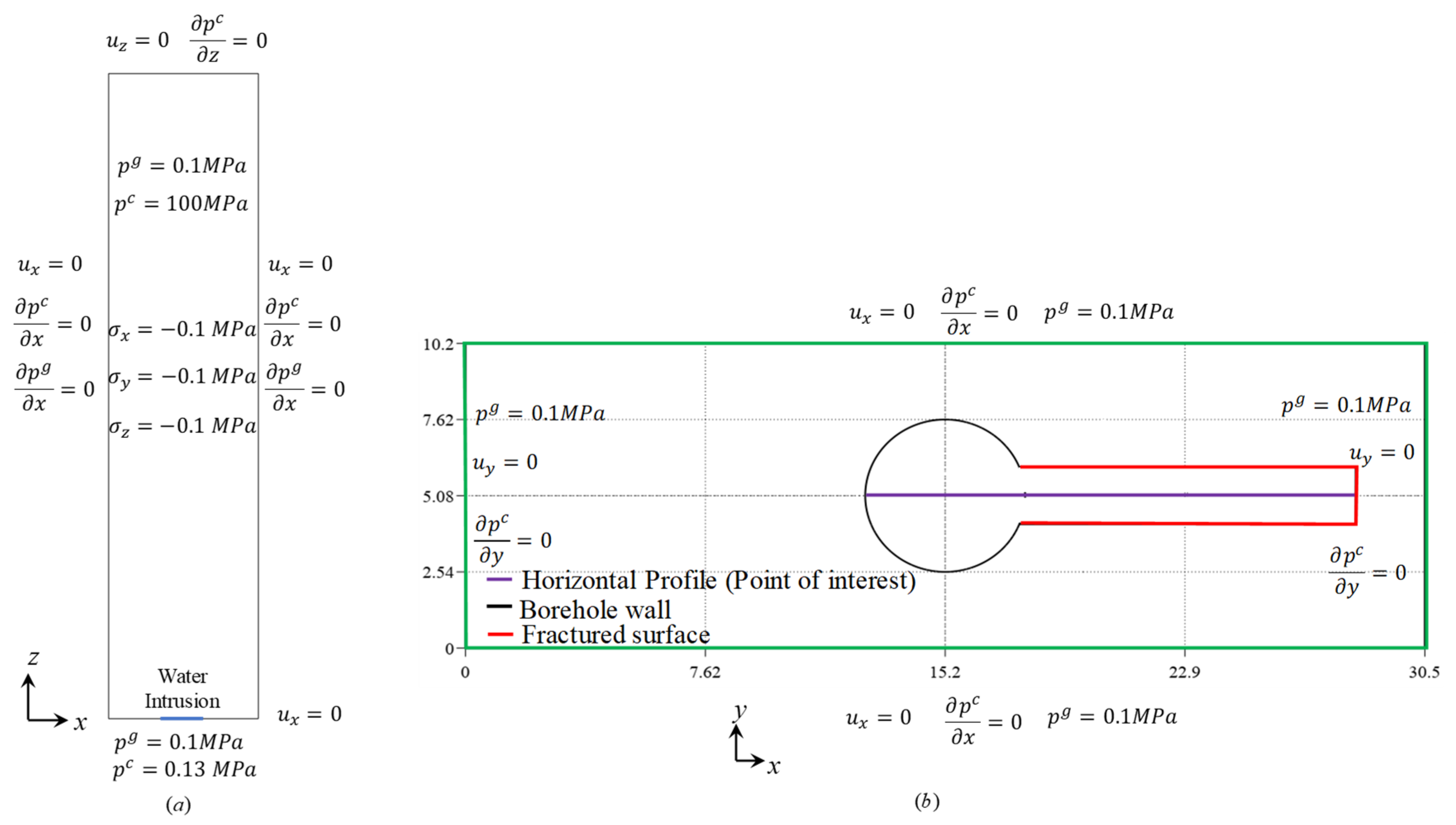
2.2.5. Initial and Boundary Conditions

Initial and boundary conditions for the finite element modeling were selected to describe a clay-filled borehole into which additional fluid is driven by pressure differences. Changes in the fluid saturation of the clay cause swelling and displacement, which induce stress changes in the clay medium and surrounding rock.

For the primary variables, the initial conditions were:

$$\mathit{u}\left(t=0\right)={\mathit{u}}_0\hspace{1em}\mathrm{in} \Omega ,$$

(15)

$$p^c\left(t=0\right)=p^{c0}\hspace{1em}\mathrm{in} \Omega ,$$

(16)

$$p^g\left(t=0\right)=p^{g0}\hspace{1em}\mathrm{in} \Omega ,$$

(17)

where subscript ‘$0$’ represents the initial state of the primary variables.

Boundary conditions were represented as:

$$\mathit{u}={\mathit{u}}_{\Gamma }\hspace{1em}\mathrm{on} {\Gamma }_u,$$

(18)

$$\mathit{\sigma }.\mathit{n}=\mathit{t}\hspace{1em}\mathrm{on} {\Gamma }_t,$$

(19)

$$p^c=p^{c\Gamma }\hspace{1em}\mathrm{on} {\Gamma }_{p^c},$$

(20)

$$p^g=p^{g\Gamma }\hspace{1em}\mathrm{on} {\Gamma }_{p^g},$$

(21)

$${\mathit{w}}_j.\mathit{n}=q^j\hspace{1em}\mathrm{on} {\Gamma }_{q^j}.$$

(22)

The boundary-applied displacement and tractions are ${\mathit{u}}_{\Gamma }$ and $\mathit{t}$, respectively. In the primary fluid variables, the superscript ‘$\Gamma$’ represents the equivalent primary variables on the surface, $\mathit{n}$ denotes the unit normal vector, and $q^j$ is the flux of the fluid phase $\left[j\in \left\{l,g\right\}\right].$ ${\Gamma }_u$, ${\Gamma }_{p^c}$, and ${\Gamma }_{p^g}$ represent the corresponding Dirichlet boundary condition. Additionally, ${\Gamma }_q$ and ${\Gamma }_t$ are the Neumann boundary conditions. For the three-phases mediums, with a domain, $\Omega$, the complementary part of the boundary, $\Gamma$, should satisfy the requirements of ${\Gamma }_u{{\displaystyle \cup }}^{ }{\Gamma }_t=\Gamma$, ${\Gamma }_{p^c}{{\displaystyle \cup }}^{ }{\Gamma }_{q^l}=\Gamma$, and ${\Gamma }_{p^g}{{\displaystyle \cup }}^{ }{\Gamma }_{q^g}=\Gamma$.

In this paper, we present two cases (see Section 2.2 and Figure 3). Details of the initial conditions and boundary conditions of those cases are shown in Figure 6. The first case is the bentonite column element test (see Figure 3a), where we restricted horizontal displacement along the lateral boundaries and at the bottom. Additionally, we also restricted vertical displacement at the top. Moreover, we considered that the top and lateral boundaries are impervious. Therefore, we only allowed bentonite swelling due to liquid intrusion (see Figure 6a) along the vertical direction, which behaves like free swelling in a confined space (see Figure 1). Along the water intrusion area, the capillary pressure and gas pressure were 0.1 and 0.13 MPa. Moreover, we also assumed that initially, the gas pressure inside the bentonite sample was equivalent to the atmospheric pressure, while the capillary pressure was 100 MPa. Therefore, due to the capillary pressure gradient, the liquid saturation increased from the bottom.

Additionally, for the swell cell-equivalent numerical modeling (see Figure 6b), we restricted the displacement along the outer boundary. We assumed that there is no flow along the exterior boundary. Additionally, in the swell cell test (see also Figure 2), we put water in the domain and sealed it. Therefore, to mimic the similar condition, we assigned the capillary pressure and gas pressure as 10 Pa and 0.1 MPa, respectively, along the wellbore wall, which corresponds to the degree of liquid saturation of 1. We also introduced capillary pressure for the bentonite, rock, fractured zone, and fracture as 95, 55, 75, and 70 MPa, respectively, while for similar sub-domains, we also assumed gas pressure as being equivalent to atmospheric pressure (0.1 MPa).

Moreover, for both cases, we also assumed that the overburden pressure (${\sigma }_z$), maximum horizontal stress (${\sigma }_x$), and minimum horizontal stress (${\sigma }_y$) are also equivalent to the atmospheric pressure.

It is noteworthy that for (i) two fluids only, (ii) the Richards flow coupled with the deformation flow and (iii) the two-phases flow coupled with the deformation flow, the number of equations and variables are 12 (see Bear and Bachmat [39]), 25 (see Anandarajah [58]), and 34, respectively (present study). In our solution algorithms, we used the linear momentum equations for (a) the solid phase (three equations), (b) liquid phase (three equations), and (c) gas phase (three equations). In Equation (1), we presented coupled linear momentum equation for the three phases. Additionally, we used three mass balance equations for three phases and their coupled form is presented in Equations (2) and (3). We also used six stress–strain relations (see Equation (9)). Moreover, assuming the symmetric conditions and small deformation theory, there are an additional six equations (see Equation (8); Anandarajah [58]). It is noteworthy that for bentonite, we considered poro-plasticity coupled with the swelling model, while other domains were modeled assuming poro-elasticity. In both cases, the number of stress–strain–displacement relation equations and variables were the same. However, depending on the poro-elasticity or poro-plasticity additional terms (e.g., swelling), their expressions were different. Additionally, we also used the Darcy’s law for liquid (three equations) and gas (three equations), where we used the absolute velocity terms to couple the solid and fluids (see Appendix A). The other four equations used included (i) the capillary pressure and saturation relation (see Appendix A, Equations (A9) and (A10)) and (ii) the three relations between the phase stress and phase density (see Appendix A, Equations (A4)–(A8) and Equations (A13)–(A15)). Thereby, we used a total of 34 equations.

Additionally, the total number of variables for the effective stress and strain were 12 (see Equation (9) and Appendix A, Equations (A5) and (A11)). For the velocity components of each phase and their absolute velocity, the total number of variables were 15. We assumed two fluids phases primary variables (the capillary pressure and gas pressure). For the effective saturation (see Equation (4)), for each phase density and porosity, we used five more variables. Thereby, for 34 variables, we used 34 equations.

2.3. Material and Fluid Properties

A total of four materials were investigated and their material properties are presented in

Table 1. Material properties of rock, bentonite, fractured zone, and fracture.

Properties	Symbol	Unit	Value
			Rock **	Bentonite *	Fractured Zone **	Fracture **
Density	$\rho$	Kg·m3	2700	1970	2000	1700
Porosity	$\phi$	---	0.01	0.279	0.3	1.0
Permeability	$\mathit{k}$	m2	1.0 × 10−17	4.3 × 10−21	1.0 × 10−15	$k_f$
Young’s Modulus	$E$	Pa	3.5 × 1010	8.6 × 106	3.5 × 107	3.5 × 106
Poisson’s ratio	$\nu$	--	0.40	0.30	0.30	0.30

Note: ** Assumed, Fracture permeability $k_f=\frac{b^2}{12}$, Aperture (b) = 200 µm, * Yi et al. [46]

. For the poro-elastic model (see Coussy [30]), the model parameters are the Young’s modulus and Poisson’s ratio. Additionally, for the plastic state model of bentonite, we obtained the MCC model parameters from Yi et al. [46], as shown in

Table 2. Modified Cam Clay model parameter of bentonite [see Yi, et al. [46] (Sample: SO-04)].

Parameter	Symbol	Unit	Value
Slope of the critical state line	$M$	-	1.84
Virgin compression index	$\lambda$	-	0.12
Swelling/recompression index	$\kappa$	-	0.024
Initial preconsolidation pressure	$p_{iso}$	MPa	2.43
Initial void ratio	$e$	-	0.6376

. Moreover, for the swelling model of bentonite, we assumed that the maximum swelling stress was 4.68 MPa, while we assumed an initial capillary pressure of bentonite of 65 MPa. We assumed the liquid phase density and viscosity were 1000 kg·m⁻³ and 1 × 10⁻³ Pa·s, respectively. For the gas phase density, we assumed the Clapeyron equation, while we assumed the gas phase viscosity was 1.8 × 10⁻⁵ Pa·s. Additionally, to present the saturation state transition between the liquid phase and gas phase, we used the data shown in Figure 7 to obtain the Brooks and Corey [42] model parameters (see Equations (4)–(6)).

We present the validation of the bentonite swelling model in Appendix D for sample SO-04 (see Yi et al. [46]).

3. Results and Discussions

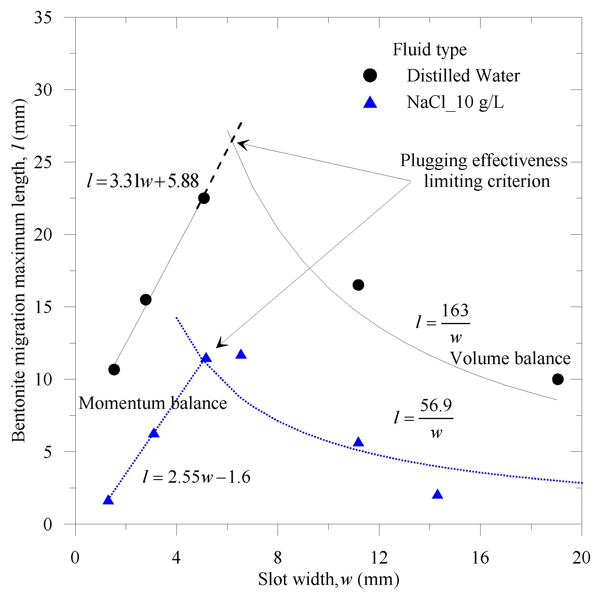
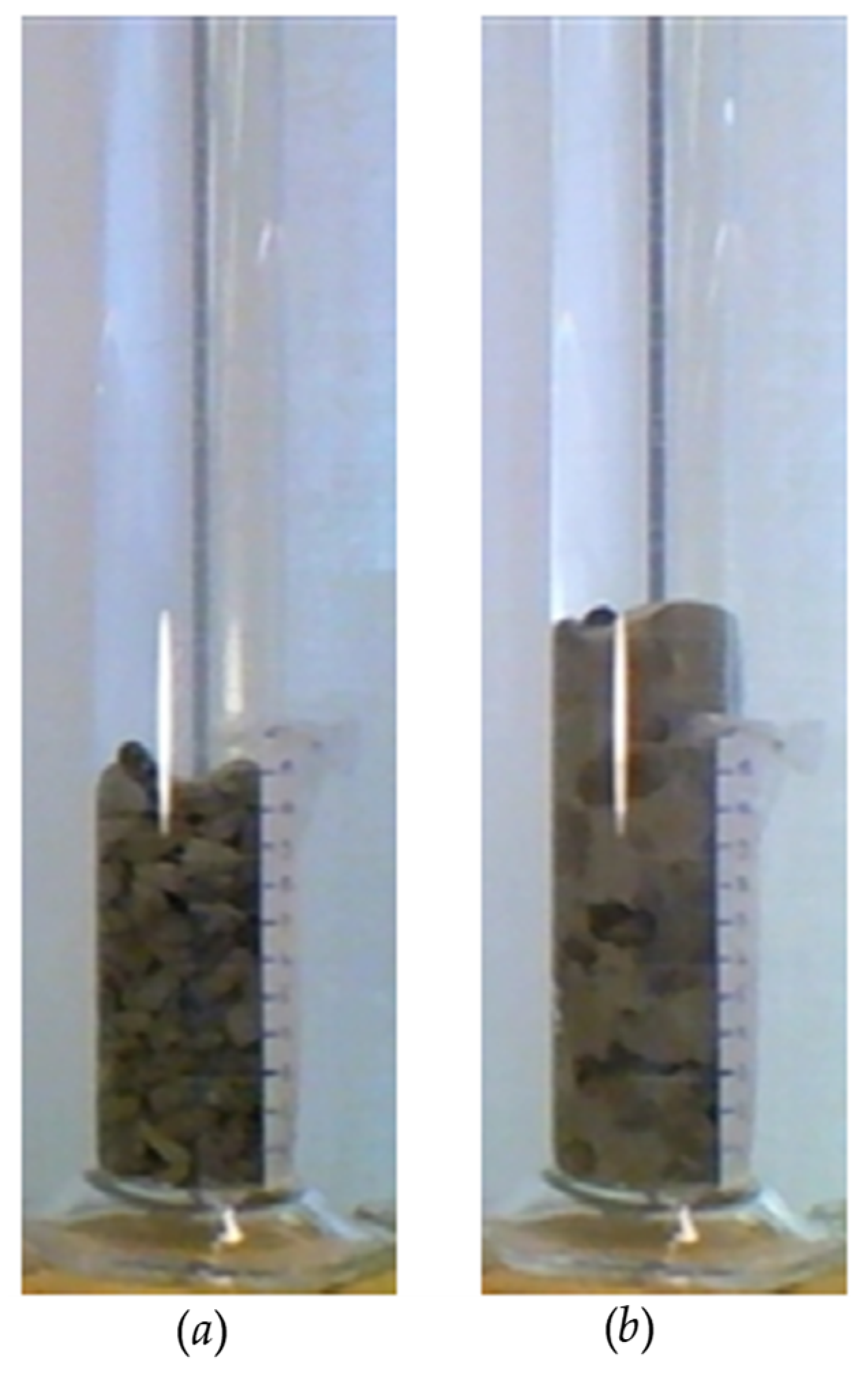
3.1. Experimental Results

We used the free swelling test of bentonite (see Section 2.1 and Figure 1), where we changed the liquid’s salinity and then measured the swelling potential. From the observation, we found that due to the change of salinity, the free bentonite swelling potential $\left(s_p\right)$ were 0.42, 0.38, 0.32, 0.25, and 0.16, respectively, representing the increase of salinity, and the value of $s_p$ decreasing, as shown in Figure 8.

In Figure 8, the salinity zero represents distilled water. We discussed earlier that the swelling potential is an indicator of the effectiveness of the developed swelling stress. Therefore, Figure 8 confirmed the importance of considering the geochemistry of the saturated fluid (see [59]).

Among others, Bolchover et al. [11], Svoboda [12], and Islam et al. [24] reported that when bentonite extrudes into a fracture (see the swell cell test experiments shown in Figure 2 in Section 2.1), two forces satisfy the equilibrium condition. They are the swelling-induced driving force and the resisting force. The bentonite extrusion stopping criterion depends on these forces’ equilibrium state, and the details are discussed in Appendix E. The driving force develops when the liquid saturation results in an increase of the swelling pressure (see also Figure 5), which pushes bentonite into the fracture. The driving force is the resultant of the swelling pressure and the fracture width (Svoboda [12]; Islam et al. [24] and see Equation (A46)). Additionally, the resisting force is the resultant of the bentonite extrusion length and the bentonite–slot contact shear strength (see Figure 2a, Figure 3a,c and Equation (A47)). According to the bentonite extrusion stopping criterion (see also Bolchover et al. [11]), bentonite migration is proportional to the slot width (or fracture aperture) (see Figure 2a and Equation (A49)). Additionally, for a fracture in a deposition hole, Kanno and Wakamatsu [9] demonstrated from the experimental results of two different bentonites (bentonite and bentonite–sand mixture) that initially, the swelling pressure increases linearly with respect to time, then it starts to decrease. Kanno and Wakamatsu [9] also presented that the swelling pressure decreases with the increase of the aperture, which is opposite to the bentonite extrusion stopping criterion. Such a decline of the swelling pressure may happen due to several reasons. Firstly, the increase of the fracture aperture results in an increase of the overall volumetric area of the fracture, where separation of bentonite happens, and Kanno and Wakamatsu [9] demonstrated such a separation from their experiments. Secondly, the fracture domain may be fully brine-saturated, and if the extrusion rate of bentonite from the host container into the fracture decreases, the existing bentonite into the fracture may start to dissolve in the brine (see also Baik et al. [60]). Thirdly, the capillary pressure gradient may decline between the host container of the bentonite and the fracture, which is also responsible for decreasing the swelling pressure (see also Figure 5), and such a phenomenon also may happen during dynamic propagation of the fracture (see also Chen et al. [61]).

In support of Kanno and Wakamatsu’s [9] findings, who showed the inverse results compared to the equilibrium theory, Islam et al. [24] proposed that during bentonite extrusion, two balance laws may work simultaneously. The first one is the momentum balance law, which supports the bentonite extrusion stopping criterion or the equilibrium state (see also Bolchover et al. [11]; Svoboda [12]). The second one is the volume balance law (see Islam et al. [24] and Appendix E in this manuscript), which is based on the swelling potential (Section 2.1 and Figure 1 and Figure 8). Additionally, for any bentonite with specified brine chemistry, fracture aperture, and reservoir condition, the intersection of the two balance laws is the limiting condition of the bentonite plugging’s effectiveness. To obtain such a limiting criterion, we developed a swell cell (see Section 2.1 and Figure 2).

Moreover, due to the gravitational force, the bentonite deposition started from the bottom of the swell cell (see Figure 2b). We observed only the final value of the bentonite migration length for different fracture widths and fluid types (e.g., distilled water, 10 g/L NaCl liquid). We performed the test at room temperature. From Figure 9, we observe that before the intersection of the momentum balance and the volume balance laws (see Appendix E), the maximum bentonite migration length is linearly proportional to the slot width, which also supports Bolchover et al. [11] and Svoboda [12]. After the bentonite plugging’s effectiveness limiting criterion, the maximum bentonite migration length decreased with respect to the slot width, which also supports Kanno and Wakamatsu [9]. It is interesting to note that in Figure 9, the ratio of the linear fittings’ line slope for the 10 g/L NaCl to the distilled water is about 0.770. Additionally, we discussed earlier from the experimental evidence of Wang et al. [23] that the free swelling potential is linearly proportional to the swelling pressure. Moreover, from Figure 8, we found that the swelling potential for the 10 g/L NaCl to the distilled water is 0.42 and 0.32, respectively, and their ratio is 0.762, which is also approximately consistent with the swell cell experimental results before the bentonite plugging’s effectiveness limiting criterion.

In the next section, we discuss the numerical modeling results. We note that in our finite element (FE) modeling, the geochemistry is beyond the scope of the present paper. Therefore, in the numerical modeling section, we ignored the chemical reaction due to fluid salinity. We only considered the distilled water as the liquid phase fluid. Thereby, we also disregarded the dissolution of bentonite in the liquid phase and assumed that the liquid phase properties are constant. We also ignored the thermal effect. Thereby, during experiments, we also disregarded evaporation of the liquid at room temperature. Additionally, in the numerical modeling section, we only considered phases (see also Figure 4) and ignored the components of each phase (see also Bear and Bachmat [39]; Lewis and Schrefler [32]). Moreover, in the swell cell test arrangement, we did not have the facilities to measure incremental bentonite migration or stress–strain or fluid phase relations with respect to time. In addition, due to the unavailability of testing facilities of unsaturated tests on bentonite, acrylic, or rock medium, we obtained numerical model parameters from the published literature (see Section 2.3).

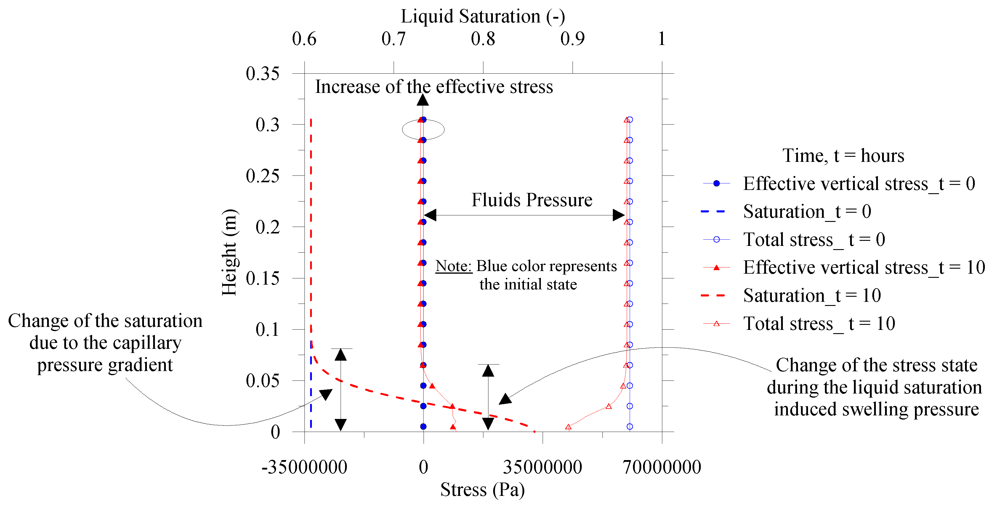
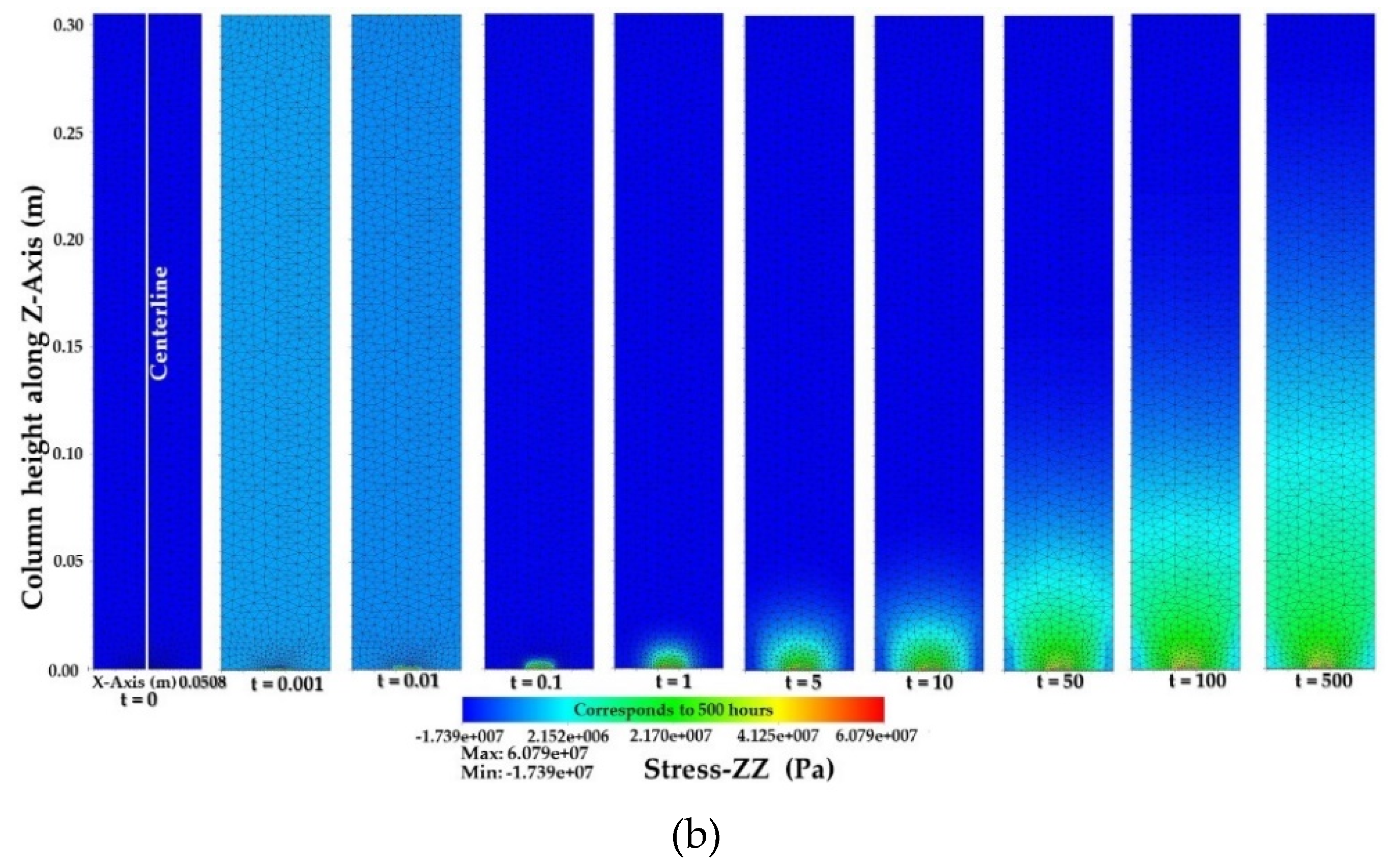
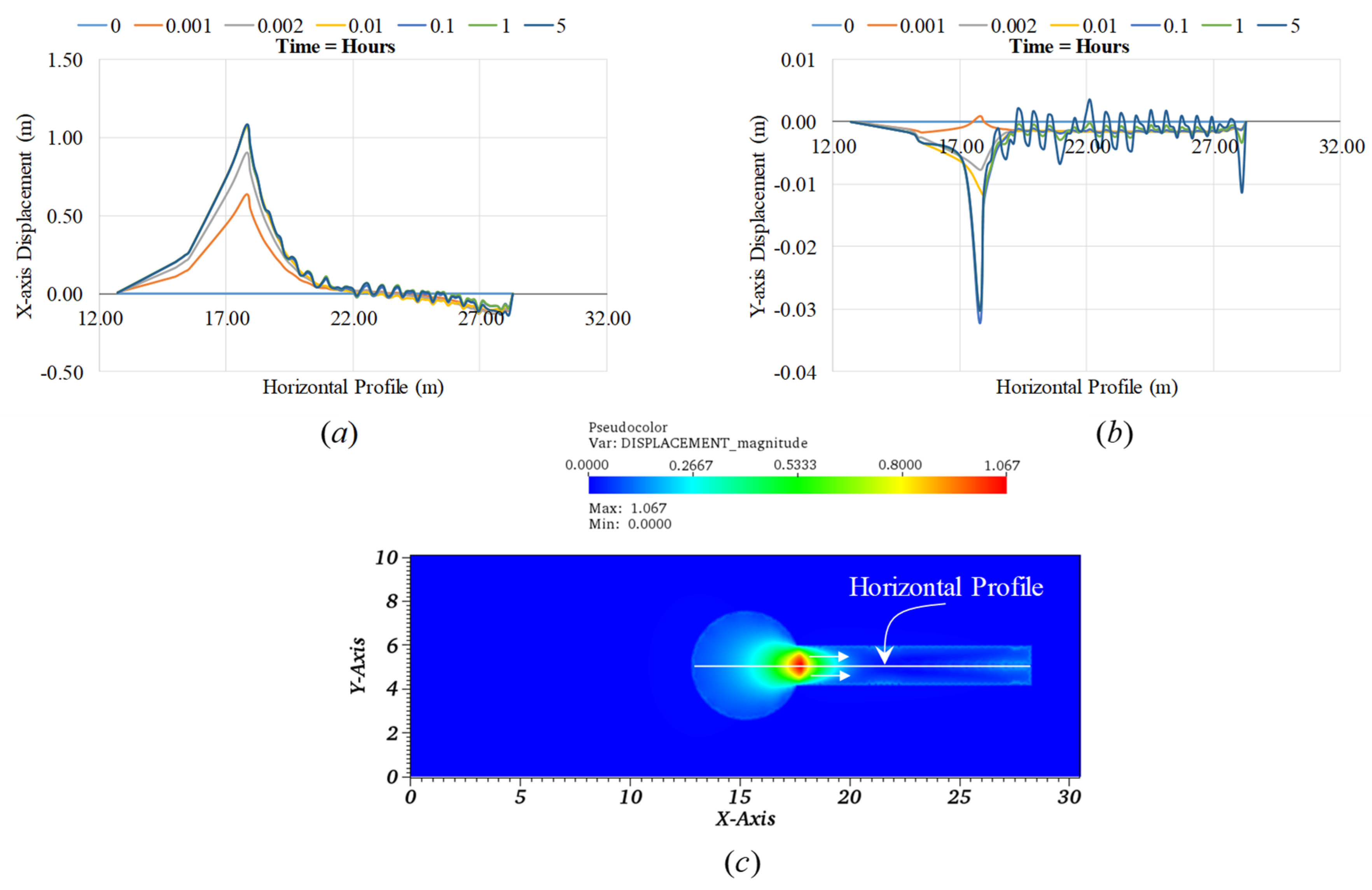
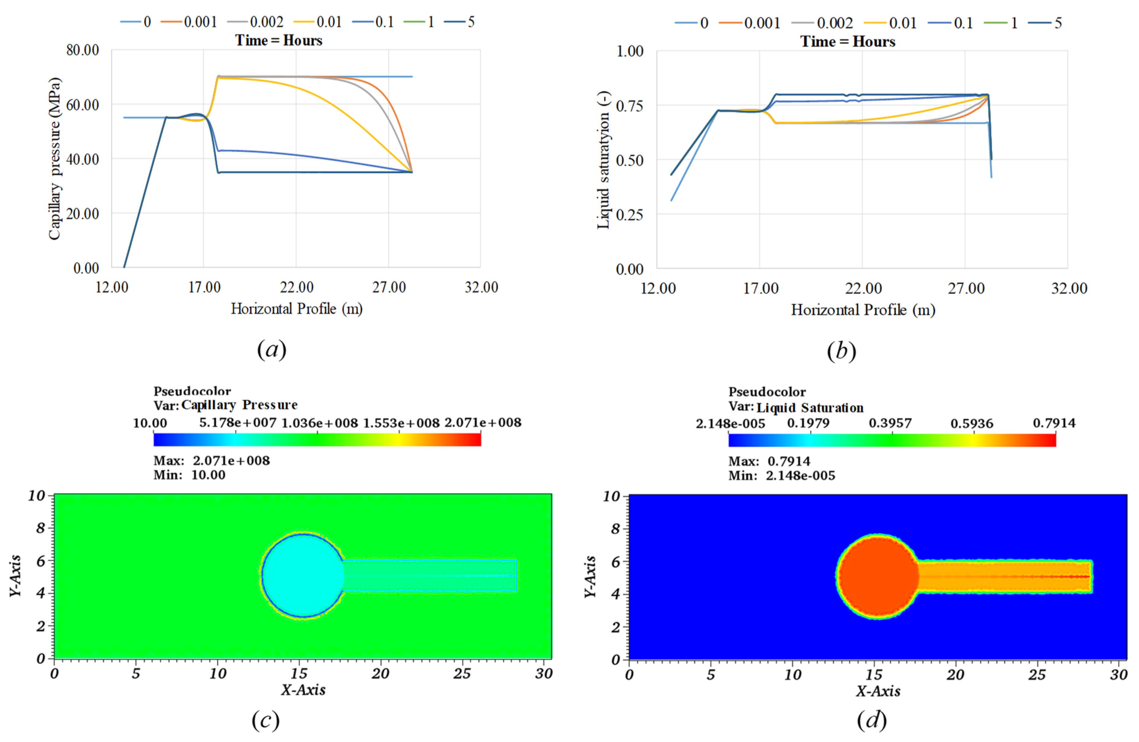
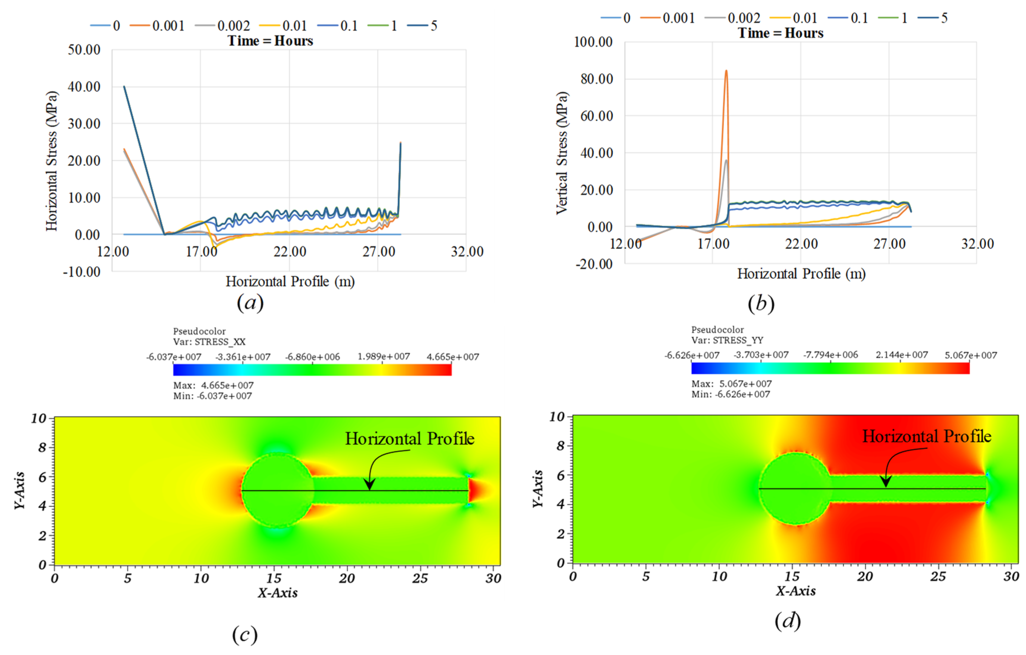
3.2. Numerical Simulation Results

In Section 2.2, we discussed two types of finite element simulations. They are bentonite column simulation and swell cell equivalent simulation. Additionally, in Figure 3, we also demonstrated the relation between the two types of simulation. The first one represents the homogeneous three-phases medium while the latter one illustrates the heterogeneous three-phases mediums. Additionally, we also discussed the justification of these numerical simulations in the earlier section (see the experimental results section). We also discussed the initial and boundary conditions of two types finite element simulations in Section 2.2.4. Moreover, we presented the material and fluid properties in Section 2.3.

In the initial state of the bentonite column element simulation (see Figure 6a), we assumed that inside the sample, the capillary pressure is high compared to the bottom boundary. We assumed that the bentonite initial water saturation is 0.28, while in the water intrusion area, the liquid saturation is 1.0 (see also Figure 6a and Figure 7a). Thereby, we introduced a high capillary pressure gradient. The capillary pressure gradient will lead to an increase in the saturation of the bentonite medium over time. Additionally, we allowed displacement and swelling pressure of bentonite to occur from the bottom of the column due to a surge of the liquid phase saturation. We also discussed details of the stress in Equations (1), (9), (11), and (A3)–(A8).

In Figure 10, we demonstrate the stress state and liquid saturation state change in the initial state condition and after 10 h. We observe that the shapes of the stress states are similar to the shape of the liquid saturation state. It is worth noting that in any confined space, bentonite swelling involves free swelling and back compaction (see Rutqvist et al. [62]; Xie et al. [63]). We considered liquid intrusion from the bottom, thereby changes of the liquid saturation and swelling-induced stress also started to change from the bottom. Among others, Birkholzer et al. [51] also demonstrated a similar finding for bentonite swelling.

In Figure 11a, we present the vertical displacement profile, and in Figure 12a, the centerline displacement with respect to time. We observed that after 0.001 h (3.6 s), the displacement profile exhibits a parabolic shape. Due to the capillary pressure gradient in the bentonite column domain and bottom boundary (see also Figure 6a), the water intrusion increases, which also changes the liquid saturation. Thereby, in the bottom of the bentonite column, an increase in the swelling pressure occurs, which accelerates the displacement profile. We also observe that as time increases, the maximum displacement at the column centerline develops at a column height of approximately 0.14 m and that the rate of change of vertical displacement is predicted to decrease significantly after 50 h. A similar trend is also observed for the stress distribution along the column height and we present them in Figure 11b and Figure 12b. Due to the induced swelling stress, at the bottom, the stress component along the z-axis (${\sigma }_z$) is high.

From Figure 13 and Figure 14, we observe that over time as the capillary pressure decreases, the liquid saturation progressively increases, which also supports Agus et al.’s [47] demonstrated laboratory experiments (see also Figure 5). The liquid saturation increase continues until an equilibrium state is achieved, or the capillary pressure gradient is negligible. Such a process is also known as the wetting process of bentonite. In this paper, we do not discuss the drying stage.

In Figure 6a, if we inverse the boundary and initial conditions, we will observe that the drying stage or wetting phase occurs in the reverse direction (e.g., from the bentonite medium to the boundary). In the wetting phase, we assigned a higher capillary pressure inside the bentonite domain, which we need to assign in the boundary to obtain the drying process. To avoid repetition of similar numerical simulations and identical illustrations, we ignored the drying state. However, in the bentonite-based borehole plugging, such a wetting and drying stage may happen depending on the bottom holes’ reservoir condition change with the course of time or due to the weathering effect (e.g., rain). Additionally, in the wetting phase and drying phase, the bentonite will swell and shrink, respectively, which is crucial for boreholes with compromised sections like a fracture. In the next section, we discuss the swell cell, where we considered a fracture in the domains.

In Figure 3a,c, we present the swell cell equivalent geometry for the numerical simulations. Additionally, in Figure 6b, we illustrate the initial and boundary conditions of the similar problem statement, while in Table 1 and Table 2 and Figure 7, we demonstrate the model parameters and material properties. Moreover, in the earlier section for the bentonite column numerical simulation, we considered the wetting process of bentonite. In the swell cell equivalent model, we also used the wetting process concept. As we discussed earlier, the main difference between the two numerical solution cases is the illustration of the three-phases homogeneous medium (e.g., bentonite column element) and the three-phases heterogeneous mediums (e.g., swell cell). Due to the application of the identical mechanisms, the capillary pressure gradient inside the bentonite domain of the swell cell (see also Figure 3a,c, and Figure 6b) increases the liquid saturation of bentonite. Thereby, the swelling pressure also increases due to the incremental liquid saturation (see Equations (7), (11), and (12) and Figure 5) and it continues until it reaches the maximum swelling pressure.

Additionally, Xie et al. [63] explain that an engineering barrier system may fail if the swelling pressure exceeds the tolerable limit of the barrier material or surrounding material. Moreover, Mielenz and King [64] also presented that the volume change in Na-montmorillonite and Ca-montmorillonite is 1400% to 2000% and 45% to 145%, respectively. In Equation (12) and Figure 5, we also present that the incremental swelling pressure is a function of the incremental liquid saturation and maximum swelling pressure. Therefore, for boreholes with fractures (e.g., swell cell equivalent field case), extra care is essential to determine the maximum swelling pressure. Otherwise, the success of borehole plugging may be jeopardized due to the developed stress through the compromised section (e.g., fracture). In such a case, prediction of the stress distribution and fluid phase saturation is essential.

In Figure 15, we present the displacement (x and y components) along the horizontal profile (see also Figure 6b) and after 5 h, the displacement profile in the x-y plane (see also Figure 3a,c). We observe that the maximum displacement is close to the wellbore center (see Figure 14a,b). After the initiation of the simulation, the displacement (x and y components) progressed sharply, then with the increase of time, the displacement magnitude decreased. After 1 h, we observed a negligible change in displacement, which represented that for the assigned initial and boundary conditions, material properties, and model parameters, the capillary pressure gradient in the domain approached the equilibrium state. Moreover, along the fracture line, we noticed oscillation in the displacement, which might be due to the thin aperture closed conduit, where, at the end, we restricted the displacement field to avoid instabilities in the numerical simulation. A similar trend is also observed in the stress distribution, which is shown in Figure 16. During the increase of liquid saturation, the stress state along the horizontal and the vertical directions will also increase until it reaches the maximum swelling pressure (see also Figure 15). Additionally, in Figure 17, we present the capillary pressure profile and liquid saturation profile, respectively, along the horizontal profile and X-Y plane after 5 h. We observed that due to the capillary suction inside of the bentonite, changes of the liquid saturation inside the bentonite domain are high compared to the fractured zone.

4. Conclusions and Discussions

To address the bentonite swelling behavior and its migration to the near-borehole crack, we performed laboratory tests, presenting an analytical model and coupled finite element model. From experiments of the free swelling test and the swell cell test, we observed that for the performance of the bentonite-based borehole plugging, liquid phase geochemistry plays a significant role in the swelling phenomena of bentonite. With the increase of salinity, the swelling potential of bentonite decreases, which also represents a decrease in bentonite expansion. Additionally, the swell cell results illustrate that for the effectiveness of the borehole plugging, there is a limiting criterion for the maximum bentonite intrusion length and fracture aperture. The analytical model also supports the swell cell results. By superimposing the momentum balance and volume balance in the analytical model, the limiting condition of the bentonite-based borehole plugging can also be found. In the momentum balance region, the maximum bentonite migration length is linearly proportional to the fracture width, which is opposite the volume balance region.

For the bentonite material model, the Modified Cam Clay model (MCC) was combined with the swelling model. The MCC model was used to capture the elasto-plastic state of the bentonite, while the swelling model was used to understand the swelling phenomena. The swelling phenomena of the bentonite model required only six parameters and five of them were identical to the MCC model. The other parameter was the maximum swelling pressure of the bentonite. All six parameters can be obtained from conventional triaxial tests, and the model does not require any fitting parameters. Additionally, in the two-phases flow model, the fluids were water and air, while the primary variables were the capillary pressure and gas pressure. During the wetting phase of bentonite, due to the capillary pressure gradient, water entered the bentonite medium, thereby increasing the liquid saturation and also increasing the swelling pressure, which is the driving force for the displacement and stress components. Additionally, we presented the validation of the bentonite model by comparing the experimental results obtained from the literature and the coupled finite element model.

In the bentonite column element test, we considered that the displacement along the x-axis is restricted. Thereby, two-phases fluids and deformation flow through porous media surrounded by the rigid body. Additionally, in the swell cell equivalent numerical simulation, rock and fractured zones also behave like rigid media like the bentonite column element test. Therefore, in the swell cell, the developed swelling pressure in the borehole forced bentonite to migrate to the near-borehole fracture. Such a migration continued until the change of the capillary pressure with respect to time was low, which is considered as the equilibrium state of the capillary pressure gradient. It is noteworthy that in practical borehole plugging, depending on the fracture zone geometry, mechanical and physical properties, and capillary pressure gradient, if bentonite migration from the borehole to the fracture zone is high, the developed stress may jeopardize the borehole plugging’s integrity. Therefore, careful attention is essential to select the bentonite type, geometry of the fracture, downhole reservoir condition, and liquid phase geochemistry.

Additionally, depending on the bentonite state of saturation, properties, and borehole reservoir environment, initially, the swelling-induced elasto-plastic state inside the borehole wall is high, which was also observed in the swell cell simulations. In this paper, we did not consider the creep of bentonite, which can be incorporated by changing Equation (7) and relevant constitutive laws (see also Islam and Gnanendran [49] and Islam et al. [48]). In addition, we presented in Equation (12) that the swelling pressure is a function of the maximum swelling pressure and liquid phase saturation. However, by changing the swelling model with respect to the density or the void ratio (see Sun [65]), it is also possible to obtain the density or the void ratio distribution. It is important to note that to incorporate the density- or void ratio-based swelling model in the coupled finite element solution, careful consideration is essential regarding the selection of fitting parameters. Otherwise, numerical convergence issues might be encountered and the consistency also needs to be considered. Moreover, we assumed constant fracture aperture, while dynamic fracture propagation also can be introduced by following Borst [66]. It is worthy to note that for the liquid phase only, the fracture propagation algorithm is relatively simple. However, for two-phases fluids, a composite heterogeneous domain, and poro-plasticity, the dynamic fracture propagation algorithm requires special attention. This is because incorporating such an algorithm may create the stress singularity problem during calculation of the internal stress vector and the stiffness matrix. In addition, in this paper, we assumed small deformation conditions (see Equation (8)), which might also need to be revised for fracture propagation.

References

1. Ide, S.T.; Friedmann, S.J.; Herzog, H.J. CO2 leakage through existing wells: Current technology and regulations. In Proceedings of the 8th Greenhouse Gas Technology Conference, Trondjhei, Norway, 19–22 June 2006; pp. 19–22. [Google Scholar]
2. Towler, B.F.; Firouzi, M.; Mortezapour, A.; Hywel-Evans, P.D. Plugging CSG wells with bentonite: Review and preliminary lab results. In Proceedings of the SPE Asia Pacific Unconventional Resources Conference and Exhibition, Brisbane, Australia, 9–11 November 2015; p. 10. [Google Scholar]
3. Yong, R.N.; Boonsinsuk, P.; Wong, G. Formulation of backfill material for a nuclear fuel waste disposal vault. Can. Geotech. J. 1986, 23, 216–228. [Google Scholar] [CrossRef]
4. Beswick, J. Status of technology for deep borehole disposal. Contract No. NP 01185 2008, 1185, 16–18. [Google Scholar]
5. Brady, P.V.; Freeze, G.A.; Kuhlman, K.L.; Hardin, E.L.; Sassani, D.C.; MacKinnon, R.J. Deep borehole disposal of nuclear waste: US perspective. In Geological Repository Systems for Safe Disposal of Spent Nuclear Fuels and Radioactive Waste, 2nd ed.; Woodhead Publishing: Cambridge, UK, 2017; pp. 89–112. [Google Scholar] [CrossRef]
6. Townsend-Small, A.; Ferrara, T.W.; Lyon, D.R.; Fries, A.E.; Lamb, B.K. Emissions of coalbed and natural gas methane from abandoned oil and gas wells in the United States. Geophys. Res. Lett. 2016, 43, 2283–2290. [Google Scholar] [CrossRef]
7. Dilmore, R.M.; Sams, J.I.; Glosser, D.; Carter, K.M.; Bain, D.J. Spatial and temporal characteristics of historical oil and gas wells in pennsylvania: Implications for new shale gas resources. Environ. Sci. Technol. 2015, 49, 12015–12023. [Google Scholar] [CrossRef] [PubMed]
8. Mitchell, A.L.; Casman, E.A. Economic incentives and regulatory framework for shale gas well site reclamation in Pennsylvania. Environ. Sci. Technol. 2011, 45, 9506–9514. [Google Scholar] [CrossRef] [PubMed]
9. Kanno, T.; Wakamatsu, H. Experimental Study on Bentonite Gel Migration from a Deposition Hole. In Proceedings of the third international conference on nuclear fuel reprocessing and waste management, RECOD′91, Sendai, Japan, 14–18 April 1991; pp. 1005–1010. [Google Scholar]
10. Tanai, K.; Matsumoto, K. A study of extrusion behavior of buffer material into fractures. Sci. Technol. Ser. 2008, 334, 57–64. [Google Scholar]
11. Bolchover, P.; Myers, T.G.; Peletier, M.A.; Ahmer, W.M. Behaviour of Bentonite Clay in Toxic Waste Barriers. In Proceedings of the European Study Group with Industry 1998 Final Reports, Southampton, UK, 22–27 March 1998; pp. 1–13. [Google Scholar]
12. Svoboda, J. The experimental study of bentonite swelling into fissures. Clay Miner. 2013, 48, 383–389. [Google Scholar] [CrossRef]
13. Kanno, T.; Iwata, Y.; Sugino, H. Modelling of bentonite swelling as solid particle diffusion. In Clay Science for Engineering; Adachi, K., Fukue, M., Eds.; CRC Press: Boca Raton, FL, USA, 2001; pp. 561–570. [Google Scholar]
14. Borrelli, R.A.; Ahn, J. Numerical modeling of bentonite extrusion and radionuclide migration in a saturated planar fracture. Phys. Chem. Earth. 2008, 33, S131–S141. [Google Scholar] [CrossRef]
15. Sanchez, M.; Gens, A.; do Nascimento Guimarães, L.; Olivella, S. A double structure generalized plasticity model for expansive materials. Int. J. Numer. Anal. Methods Geomech. 2005, 29, 751–787. [Google Scholar] [CrossRef]
16. Helmig, R. Multiphase Flow and Transport Processes in the Subsurface: A Contribution to the Modeling of Hydrosystems; Springer: New York, NY, USA, 1997. [Google Scholar]
17. Kueper, B.H.; Frind, E.O. Two-phase flow in heterogeneous porous media: 1. Model development. Water Resour. Res. 1991, 27, 1049–1057. [Google Scholar] [CrossRef]
18. Aziz, K.; Settari, A. Petroleum Reservoir Simulation; Applied Science Publishers Ltd.: London, UK, 1979. [Google Scholar]
19. Park, C.H.; Böttcher, N.; Wang, W.; Kolditz, O. Are upwind techniques in multi-phase flow models necessary? J. Comput. Phys. 2011, 230. [Google Scholar] [CrossRef]
20. Shad, S.; Maini, B.B.; Gates, I.D. Effect of gap and flow orientation on two-phase flow in an oil-wet gap: Relative permeability curves and flow structures. Int. J. Multiphase Flow 2013, 57, 78–87. [Google Scholar] [CrossRef]
21. Snow, D.T. Anisotropie permeability of fractured media. Water Resour. Res. 1969, 5, 1273–1289. [Google Scholar] [CrossRef]
22. Witherspoon, P.A.; Wang, J.S.Y.; Iwai, K.; Gale, J.E. Validity of Cubic Law for fluid flow in a deformable rock fracture. Water Resour. Res. 1980, 16, 1016–1024. [Google Scholar] [CrossRef]
23. Wang, Q.; Tang, A.M.; Cui, Y.-J.; Delage, P.; Gatmiri, B. Experimental study on the swelling behaviour of bentonite/claystone mixture. Eng. Geol. 2012, 124, 59–66. [Google Scholar] [CrossRef]
24. Islam, M.N.; Upadhyay, R.; Wehner, C.; Bunger, A.P. Experimental demonstration of mechanisms for effective near-borehole crack plugging with bentonite (ID: 19636). In Proceedings of the American Nuclear Society (ANS-2017), International High-Level Radioactive Waste Management (IHLRWM 2017), Charlotte, NC, USA, 9–13 April 2017; pp. 1–5. [Google Scholar]
25. Kolditz, O.; Bauer, S.; Bilke, L.; Böttcher, N.; Delfs, J.O.; Fischer, T.; Görke, U.J.; Kalbacher, T.; Kosakowski, G.; McDermott, C.I.; et al. OpenGeoSys: An open-source initiative for numerical simulation of thermo-hydro-mechanical/chemical (THM/C) processes in porous media. Environ. Earth Sci. 2012, 67, 589–599. [Google Scholar] [CrossRef]
26. Geuzaine, C.; Remacle, J.-F. Gmsh: A 3-D finite element mesh generator with built-in pre- and post-processing facilities. Int. J. Numer. Methods Eng. 2009, 79, 1309–1331. [Google Scholar] [CrossRef]
27. Bethel, E.W.; Childs, H.; Hansen, C. High Performance Visualization: Enabling Extreme-Scale Scientific Insight; CRC Press: Boca Raton, FL, USA, 2016. [Google Scholar]
28. Roscoe, K.H.; Burland, J.B. On the generalized stress-strain behavior of wet clay. In Engineering Plasticity; Heyman, J., Leckie, F.A., Eds.; Cambridge University Press: Cambridge, UK, 1968; pp. 535–609. [Google Scholar]
29. Rutqvist, J. Coupled Thermal-Hydrological-Mechanical Analysis with the Framework of DECOVALEX-THMC in ‘DECOVALEX-THMC Task D: Long-Term Permeability/Porosity Changes in the EDZ and Near Field Due to THM and THC Processes in Volcanic and Crystaline-Bentonite Systems’ by Birkholzer, J. et al. (2005); Lawrence Berkeley National Laboratory: Berkeley, CA, USA, 2005; pp. 204–249. [Google Scholar]
30. Coussy, O. Poromechanics; John Wiley and Sons: Hoboken, NJ, USA, 2004. [Google Scholar]
31. Zienkiewicz, O.C.; Taylor, R.L.; Zhu, J.Z. The Finite Element Method: Its Basis and Fundamentals, 6th ed.; Elsevier: New York, NY, USA, 2005. [Google Scholar]
32. Lewis, R.W.; Schrefler, B.A. The Finite Element Method in the Static and Dynamic Deformation and Consolidation of Porous Media, 2nd ed.; John Wiley & Sons: New York, NY, USA, 1998. [Google Scholar]
33. Ehlers, W.; Bluhm, J. Porous Media: Theory, Experiments and Numerical Applications; Springer: New York, NY, USA, 2002. [Google Scholar]
34. Potts, D.M.; Zdravkovic, L. Finite Element Analysis in Geotechnical Engineering: Theory; Thomas Telford: Heron Quay, London, UK, 1999. [Google Scholar]
35. Kolditz, O.; Gorke, U.-J.; Shao, H.; Wang, W. Thermo-Hydro-Mechanical-Chemical Processes in Fractured Porous Media: Benchmarks and Examples; Springer: Heidelberg, Germany, 2012. [Google Scholar]
36. Chen, Z.; Huan, G.; Ma, Y. Computational Methods for Multiphase Flows in Porous Media; Society for Industrial and Applied Mathematics: Philadelphia, PA, USA, 2006. [Google Scholar]
37. Paniconi, C.; Putti, M. A comparison of Picard and Newton iteration in the numerical solution of multidimensional variably saturated flow problems. Water Resour. Res. 1994, 30, 3357–3374. [Google Scholar] [CrossRef]
38. Darcy, H. Les Fontaines Publiques de la Ville de Dijon; Paris: Dalmont, 1856. Available online: https://gallica.bnf.fr/ark:/12148/bpt6k624312.image (accessed on 24 November 2019).
39. Bear, J.; Bachmat, Y. Introduction to Modeling of Transport Phenomena in Porous Media; Kluwer Academic Publishers: London, UK, 1990; Volume 4. [Google Scholar]
40. Terzaghi, K. Theoretical Soil Mechanics; Wiley: New York, NY, USA, 1943. [Google Scholar]
41. Fredlund, D.G.; Rahardjo, H. Soil Mechanics for Unsaturated Soils; John Wiley & Sons, Inc.: New York, NY, USA, 1993. [Google Scholar]
42. Brooks, R.H.; Corey, A.T. Hydraulic Properties of Porous Media, Hydrology Papers 3; Colorado State University: Fort Collins, CO, USA, 1964; p. 27. [Google Scholar]
43. Burdine, N.T. Relative Permeability Calculations from Pore Size Distribution Data. Pet. Trans. AIME 1953, 198, 71–78. [Google Scholar] [CrossRef]
44. Schofield, A.N.; Wroth, P. Critical State Soil Mechanics; McGrawHill: London, UK, 1968. [Google Scholar]
45. Desai, C.; Siriwardane, H.J. Constitutive Laws For Engineering Materials; Prentice-Hall: Upper Saddle River, NJ, USA, 1984. [Google Scholar]
46. Yi, H.; Wang, W.; Kolditz, O.; Shao, H.; Zhou, H. Hydromechanical modelling of the SEALEX experiments. Environ. Earth Sci. 2017, 76, 737. [Google Scholar] [CrossRef]
47. Agus, S.S.; Arifin, Y.F.; Tripathy, S.; Schanz, T. Swelling pressure–suction relationship of heavily compacted bentonite–sand mixtures. Acta Geotech. 2013, 8, 155–165. [Google Scholar] [CrossRef]
48. Islam, M.N.; Gnanendran, C.T.; Massoudi, M. Finite element simulations of an elasto-viscoplastic model for clay. Geosciences 2019, 9, 145. [Google Scholar] [CrossRef]
49. Islam, M.N.; Gnanendran, C.T. Elastic-viscoplastic model for clays: Development, validation, and application. J. Eng. Mech. 2017, 143. [Google Scholar] [CrossRef]
50. Richards, L.A. Capillary conduction of liquids through porous mediums. J. Appl. Phys. 1931, 1, 318–333. [Google Scholar] [CrossRef]
51. Birkholzer, J.; Rutqvist, J.; Sonnenthal, E.; Barr, D. DECOVALEX-THMC Task D: Long-Term Permeability/Porosity Changes in the EDZ and Near Field due to THM and THC Processes in Volcanic and Crystaline-Bentonite Systems, Status Report October 2005; Ernest Orlando Lawrence Berkeley NationalLaboratory: Berkeley, CA, USA, 2005. [Google Scholar]
52. Wang, W.; Rutqvist, J.; Görke, U.-J.; Birkholzer, J.T.; Kolditz, O. Non-isothermal flow in low permeable porous media: A comparison of Richards’ and two-phase flow approaches. Environ. Earth Sci. 2011, 62, 1197–1207. [Google Scholar] [CrossRef]
53. Yih, C.-S. Fluid Mechanics: A Concise Introduction to The Theory [see Equation 341]; McGraw-Hill: New York, NY, USA, 1969. [Google Scholar]
54. Bear, J.; Berkowitz, B. Groundwater flow and pollution in fractured rock aquifers. Developments in Hydraulic Engineering; Novak, P., Ed.; Elsevier: New York, NY, USA, 1987; Volume 4, pp. 175–238. [Google Scholar]
55. Fourar, M.; Bories, S. Experimental study of air-water two-phase flow through a fracture (narrow channel). Int. J. Multiphase Flow 1995, 21, 621–637. [Google Scholar] [CrossRef]
56. Oron, A.P.; Berkowitz, B. Flow in rock fractures: The local cubic law assumption reexamined. Water Resour. Res. 1998, 34, 2811–2825. [Google Scholar] [CrossRef]
57. Crandall, D.; Moore, J.; Gill, M.; Stadelman, M. CT scanning and flow measurements of shale fractures after multiple shearing events. Int. J. Rock Mech. Min. Sci. 2017, 100, 177–187. [Google Scholar] [CrossRef]
58. Anandarajah, A. Computational Methods in Elasticity and Plasticity Solids and Porous Media; Springer: Berlin, Germany, 2010. [Google Scholar]
59. Karnland, O. Bentonite swelling pressure in strong NaCl Solutions: Correlation of model calculations to experimentally determined data. (No. POSIVA-98-01); Posiva Oy: Eurajjoki, Finland, 1998. [Google Scholar]
60. Baik, M.-H.; Cho, W.-J.; Hahn, P.-S. Erosion of bentonite particles at the interface of a compacted bentonite and a fractured granite. Eng. Geol. 2007, 91, 229–239. [Google Scholar] [CrossRef]
61. Chen, Y.-G.; Jia, L.-Y.; Ye, W.-M.; Chen, B.; Cui, Y.-J. Advances in experimental investigation on hydraulic fracturing behavior of bentonite-based materials used for HLW disposal. Environ. Earth Sci. 2016, 75, 787. [Google Scholar] [CrossRef]
62. Rutqvist, J.; Börgesson, L.; Chijimatsu, M.; Nguyen, T.S.; Jing, L.; Noorishad, J.; Tsang, C.F. Coupled thermo-hydro-mechanical analysis of a heater test in fractured rock and bentonite at Kamaishi Mine—comparison of field results to predictions of four finite element codes. Int. J. Rock Mech. Min. Sci. 2001, 38, 129–142. [Google Scholar] [CrossRef]
63. Xie, M.; Wang, W.; De Jonge, J.; Kolditz, O. Numerical modelling of swelling pressure in unsaturated expansive elasto-plastic porous media. Transp. Porous Media 2007, 66, 311–339. [Google Scholar] [CrossRef]
64. Mielenz, R.C.; King, M.E. Physical-Chemical properties and engineering performance of clays. Clays Clay Miner. 1952, 1, 196–254. [Google Scholar] [CrossRef]
65. Sun, D.A.; Sun, W.; Fang, L. Swelling characteristics of Gaomiaozi bentonite and its prediction. J. Rock Mech. Geotech. Eng. 2014, 6, 113–118. [Google Scholar] [CrossRef] [Green Version]
66. Borst, R. Computational Methods for Fracture in Porous Media: Isogeometric and Extended Finite Element Methods; Elsevier: Amsterdam, The Netherlands, 2018. [Google Scholar]
67. Allen III, M.B.; Behie, G.A.; Trangenstein, J.A. Multiphase Flow in Porous Media: Mechanics, Mathematics and Numerics; Springer: Berlin, Germany, 1988. [Google Scholar]
68. Kwasniewski, M.; Li, X.; Takahashi, M. True triaxial Testing of Rocks; Taylor and Francis Group, CRC Press: London, UK, 2013. [Google Scholar]
69. Sheng, D.; Sloan, W.S.; Yu, S.H. Aspects of finite element implementation of critical state models. Comput. Mech. 2000, 26, 185–196. [Google Scholar] [CrossRef]
70. Habib, P. Influence of the variation of the average principal stress upon the shearing strength of soils. Proceedings of 3rd International Conference on Soil Mechanics and Foundation Engineering, Zurich, Switzerland, 16–27 August 1953; Volume 1, pp. 131–136. [Google Scholar]
71. Prashant, A.; Penumadu, D. A laboratory study of normally consolidated kaolin clay. Can. Geotech. J. 2005, 42, 27–37. [Google Scholar] [CrossRef]
72. Wood, W.L. Practical time-stepping schemes; Oxford University Press: Oxford, UK, 1990. [Google Scholar]
73. Wang, Q.; Cui, Y.-J.; Tang, A.M.; Barnichon, J.-D.; Saba, S.; Ye, W.-M. Hydraulic conductivity and microstructure changes of compacted bentonite/sand mixture during hydration. Eng. Geol. 2013, 164, 67–76. [Google Scholar] [CrossRef]
74. Vogel, P.; Mabmann, J.; Ziefle, G.; Yi, H.; Wang, W.; Zhou, H. Chapter 7: Hydro-Mechanical (Consolidation) Proceses. In Thermo-Hydro-Mechanical-Chemical Processes in Fractured Porous Media: Modelling and Benchmarking; Kolditz, O., Gorke, U.-J., Shao, H., Wang, W., Bauer, S., Eds.; Springer: Berlin, Germany, 2016. [Google Scholar]
75. Helwany, S. Applied Soil Mechanics with Abaqus Applications; John Wiley & Sons: Hoboken, NJ, USA, 2007. [Google Scholar]
Figure 1. Free swelling of bentonite: (a) 0 h and (b) after 24 h.
Geosciences 09 00495 g001
Figure 2. (a) Schematic representation of the swell cell in the cross-section (x-y plane) and (b) the bentonite extrusion in the swell cell (see also Islam et al. [24]).
Geosciences 09 00495 g002
Figure 3. Finite element mesh for bentonite extrusion to near-borehole fracture: (a) 3D section, (b) bentonite column element along the x-z plane (axisymmetric section), and (c) cross-section along the x-y plane.
Geosciences 09 00495 g003
Figure 4. Representative elementary volume for a three-phase system.
Geosciences 09 00495 g004
Figure 5. Swelling pressure vs. capillary pressure relation and degree of saturation vs. capillary pressure relation (see Agus et al. [47]).
Geosciences 09 00495 g005
Figure 6. Initial conditions and boundary conditions: (a) The bentonite column element geometry; and (b) the swell cell-equivalent geometry.
Geosciences 09 00495 g006
Figure 7. Relative permeability–saturation and capillary pressure–saturation relations of (a) bentonite and (b) rock, fractured zone, and fracture [51].
Geosciences 09 00495 g007
Figure 8. Effects of the liquid salinity on the swelling potential of bentonite (see Islam et al. [24]).
Geosciences 09 00495 g008
Figure 9. Relations between the bentonite migration maximum length and the slot width (see also Islam et al. [24]).
Geosciences 09 00495 g009
Figure 10. At the initial state and 10-h illustration of the stress states and liquid phase saturation.
Geosciences 09 00495 g010
Figure 11. Along the x-z plane (a) the displacement profile and (b) the vertical stress distribution, in the bentonite column due to liquid infiltration-induced swelling.
Geosciences 09 00495 g011aGeosciences 09 00495 g011b
Figure 12. Along the z-axis centerline: (a) the displacement profile and (b) the vertical stress distribution, in the bentonite column due to liquid infiltration-induced swelling.
Geosciences 09 00495 g012
Figure 13. Along the x-z plane: (a) the liquid saturation profile and (b) capillary pressure distribution, in the bentonite column due to liquid infiltration-induced swelling.
Geosciences 09 00495 g013
Figure 14. Along the z-axis centerline: (a) the displacement profile and (b) vertical stress distribution, in the bentonite column due to liquid infiltration-induced swelling.
Geosciences 09 00495 g014
Figure 15. The displacement profile (see also Figure 6b): (a) along the horizontal profile X-component, (b) along the horizontal profile Y-component, and (c) X-Y plane after 5 h.
Geosciences 09 00495 g015
Figure 16. Along the horizontal profile: (a) the horizontal stress and (b) vertical stress, and along the X-Y plane after 5 h, (c) the horizontal stress and (d) the vertical stress.
Geosciences 09 00495 g016
Figure 17. Along the horizontal profile: (a) the capillary pressure, (b) the liquid phase saturation, and along the X-Y plane after 5 h: (c) the capillary pressure and (d) the liquid saturation.
Geosciences 09 00495 g017