Fluid Flow Analysis in Fractured Rock Mass by Data Integration of Digital Outcrop Model and Discrete Fracture Network (DFN)

Abstract

Fracture characterization is crucial to constrain a realistic subsurface reservoir model. They are key elements, affecting fluid flow, permeability and consequently recovery factor and productivity. Considering a proper assessment of fracture network from subsurface investigation is often difficult; in recent years, the application of Digital Photogrammetry (DP) has become popular for fracture network characterization. In this paper, we combined DP and Discrete Fracture Network modeling (DFN) to assess the fluid circulation analysis of the Monte Antola Formation (Northern Apennines, Italy). Thanks to the application of DP, it is possible to reconstruct Digital Outcrop Models (DOMs) and acquire high-precision fracture measurements such as size, location, and orientation. Utilizing quantitative measurements, we performed DFNs to simulate rock mass permeability. The primary findings from the DFNs indicate that fluid circulation is primarily influenced by (1) regions with a high density of fractures, which are associated with the primary structural features observed throughout the study area, and (2) locally, by the orientation of the dominant and persistent fracture set. The proposed approach highlights the importance of the use of DOMs for better reconstruction of the fracture network and defining an important number of relevant parameters; such quantitative information remarkably improves the reliability of DFNs.

1. Introduction

The severe drought that affected Northern Italy, as well as large areas of Europe, in Spring and Summer 2022 shows that water resources may be critical in the future [1,2], especially in mountainous areas where freshwater supply is strongly dependent on snow melt [3,4]. Therefore, management of water resources should be improved by enhancing water recovery from different sources. In this context, the characterization of fractured rock masses could be critical to fully understand the subsurface flow and, therefore, to better manage water resources, ensuring a long-term and sustainable source of freshwater.

Fractures have an important role in the hydrological properties of rock mass [5,6,7,8]; generally, they influence permeability, affecting fluid flow. Therefore, their characterization has major implications not only for water supply but also for several industrial applications, such as hydrocarbon production, geothermal energy, hazardous waste disposal and carbon capture usage and storage (CCUS) (e.g., [9,10,11,12,13,14,15,16]). Therefore, the geometric and spatial characterization of fractures is of primary importance to understand how they can influence the fluid flow of rock masses [17,18,19,20,21,22].

Developments in computer geology have led to the integration of fractures in 3D geological models, creating the so-called Discrete Fracture Network (DFN) models. These models allow for the simulation of fracture network distribution on large rock volumes. The term DFN indicates a computation model expressed by the geometrical properties of the fractures and the topological relationships between fracture sets [7,23,24]. DFN can be a powerful tool for the prediction of fluid pathways in fractured rock masses. Whereas in literature, the term DFN can be used to express several kinds of fracture network models [7], such as deterministic (defined by the fracture mapped) and geomechanical-grown (defined by the rock properties and stress-field), in this work, the term DFN refers to the stochastic fracture network model as conventionally used.

The stochastic, or probabilistic, fracture network model is widely used in geo-engineering and fluid-flow studies (e.g., [25,26,27,28,29,30]) due to the awkwardness in achieving a complete analysis of the 3D rock fracture network [31]. During the analysis of complex geological systems such as fracture networks, it is difficult to avoid uncertainties; therefore, the use of single-valued predictions from deterministic methods can lead to extremely wrong results [7]. Instead, the probabilistic nature of DFN could be considered an advantage because it allows for obtaining more than one prediction, thereby addressing the geological uncertainties [7,32].

DFN modeling necessitates the characterization of fracture properties (e.g., orientation, length, intensity, aperture, termination) and their density distribution functions (e.g., normal, log-normal, exponential distributions) along with their associated parameters (e.g., mean, standard deviation, minimum, maximum, K-Fisher coefficient) to facilitate Monte Carlo simulations of fracture networks [25,28]. Consequently, the greater the accuracy and representativeness of the fracture data, the more representative the resulting DFN models become.

A proper characterization of subsurface fracture network is often difficult and expensive, since it mostly relies on wellbore investigation [15,33,34]. While the expenses for this kind of investigation can easily be covered by oil and gas companies, those working on water supplies often find it more difficult to afford them. Moreover, wellbore investigations are often limited in spacing and resolution [35] and can be affected by orientation biases [36] and, consequently, can lack important information about the fracture network, such as spatial intensity variability. Therefore, the study of surface outcrop analogs becomes of primary importance for the characterization of the subsurface fracture network.

Frequently, the analysis of fractured rock outcrops using traditional manual field measurements can be constrained by limitations that hinder the collection of data. These limitations may include the limited presence and accessibility of rock outcrops [37] and their unfavorable orientation [20,38]). Moreover, field-manual measurements could be affected by biases (e.g., orientation and truncation biases) due to the sampling technique (scanline, window, etc.) or to the local variation in orientation of measured features (waved/undulated surface). Previous studies [37,39] have shown that the use of digital photogrammetry for the development of Digital Outcrop Models (DOMs) helps to obtain more accurate parameters of rock discontinuity features (e.g., bedding and fractures). In previous works (e.g., [40,41,42,43,44,45]), we extensively demonstrated that DOMs help to overcome the limitations of traditional geological fieldwork, allowing the acquisition of a large quantitative fracture dataset.

In this paper, we present a fluid flow analysis of a fractured rock mass performed by a combination of DOMs and DFN modeling: DOMs allow a more statistically robust constraint of fracture network parameters, consequently increasing the reliability of DFN models. The aim of the paper is twofold: (1) analyze how DOMs and DFN modeling could help to better understand the fluid flow in a heterogeneous and structurally complex formation; and (2) present a methodology to predict the preferable orientation of the flow. We tested this methodology in the Upper Staffora Valley (Northern Apennines, Italy), where the Monte Antola Formation, a fractured flysch formation, extensively crops out.

2. Study Area and Geological Setting

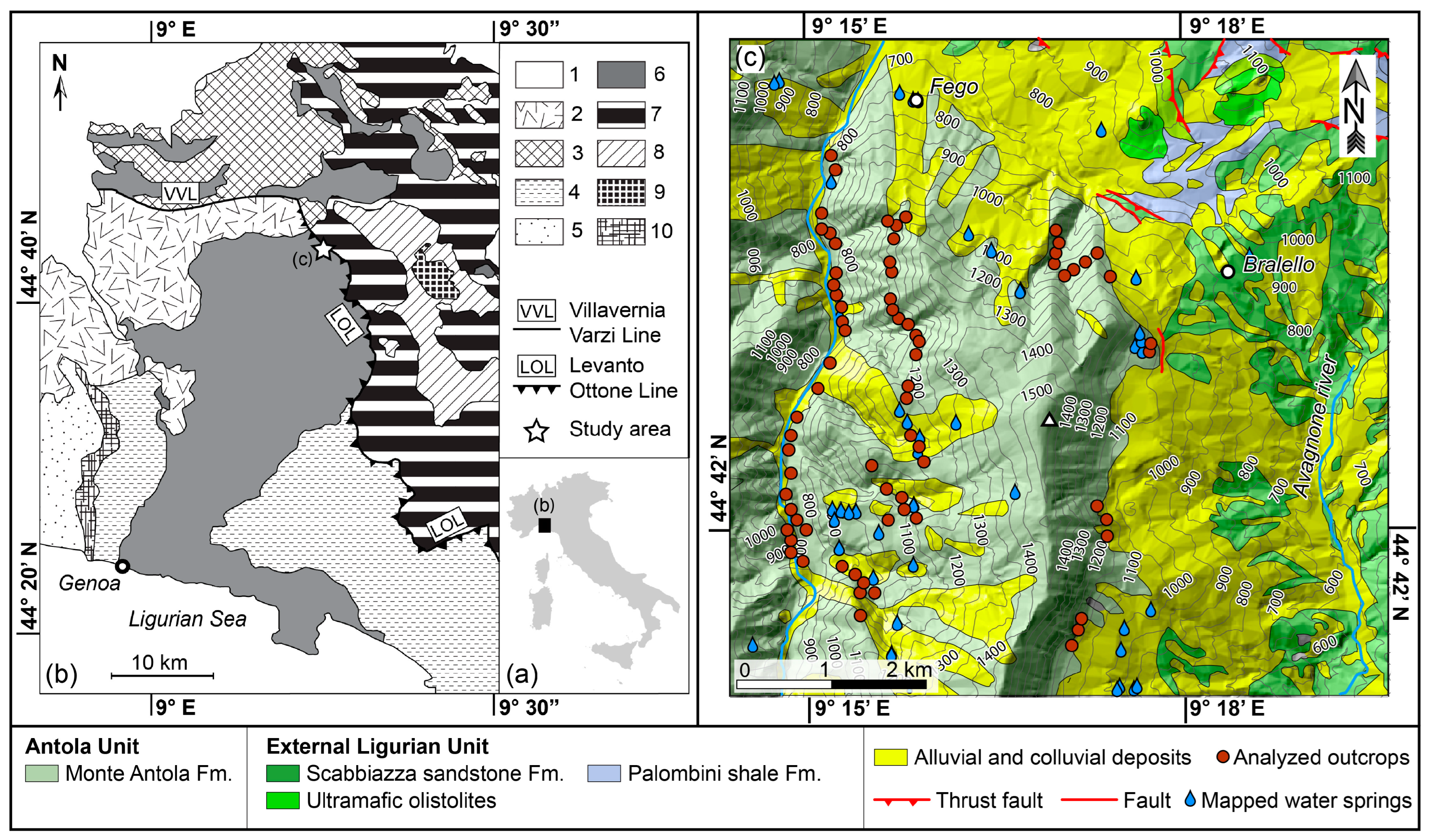
The study area is located in the North-Western Apennines, 50 km north of the city of Genoa (Figure 1).

The outcropping Monte Antola Formation, belonging to the Antola Unit (AU), crops out extensively in the study area, and it is tectonically deformed due to a complex structural evolution [47] developed under very low-grade metamorphic conditions (e.g., diagenesis-anchizone) [48]. Stratigraphically, the AU succession can be subdivided from the bottom to the top as follows [47,49,50]:

• Montoggio Shale: Varicolored hemipelagic shales (Late Cenomanian-Early Turonian);
• Gorreto Sandstone: Thin-bedded, siliciclastic and carbonatic turbidites (Early Campanian);
• Monte Antola Formation: Calcareous turbidite (Early Campanian-Early Maastrichtian);
• Bruggi-Selvapiana Formation: Siliciclastic-calcareous turbidite (Early Maastrichtian-Late Maastrichtian);
• Pagliaro Shale: Thin-bedded sandstone and calcareous turbidites alternated with shales (Late Maastrichtian-Late Paleocene).

The Antola Unit is topped by the Tertiary Piedmont Basin, a wedge-top basin located on top of the junction between the Western Alps and the Northern Apennines, which is characterized by a continuous deposition from the Mid Eocene (Monte Piano Marls) to the Late Miocene [51].

The study area, as well as the studied outcrops, is shaped in the Monte Antola Formation. In general, the Monte Antola Formation is composed of dominantly turbiditic calcareous graded beds, calcareous sandstones, sandstones and marlstones, with rare intervening thin, carbonate-free graded layers or uniformly fine-grained shale. The formation is interpreted as a deep-sea basin plain deposit, with local lateral facies variations, which range from proximal thick-bedded turbidites to distal turbidites with predominantly thickening upward cycles and a high percentage of pelites. The thickness of the more competent beds varies, ranging between 10 cm and 2 m [47].

3. Methodology

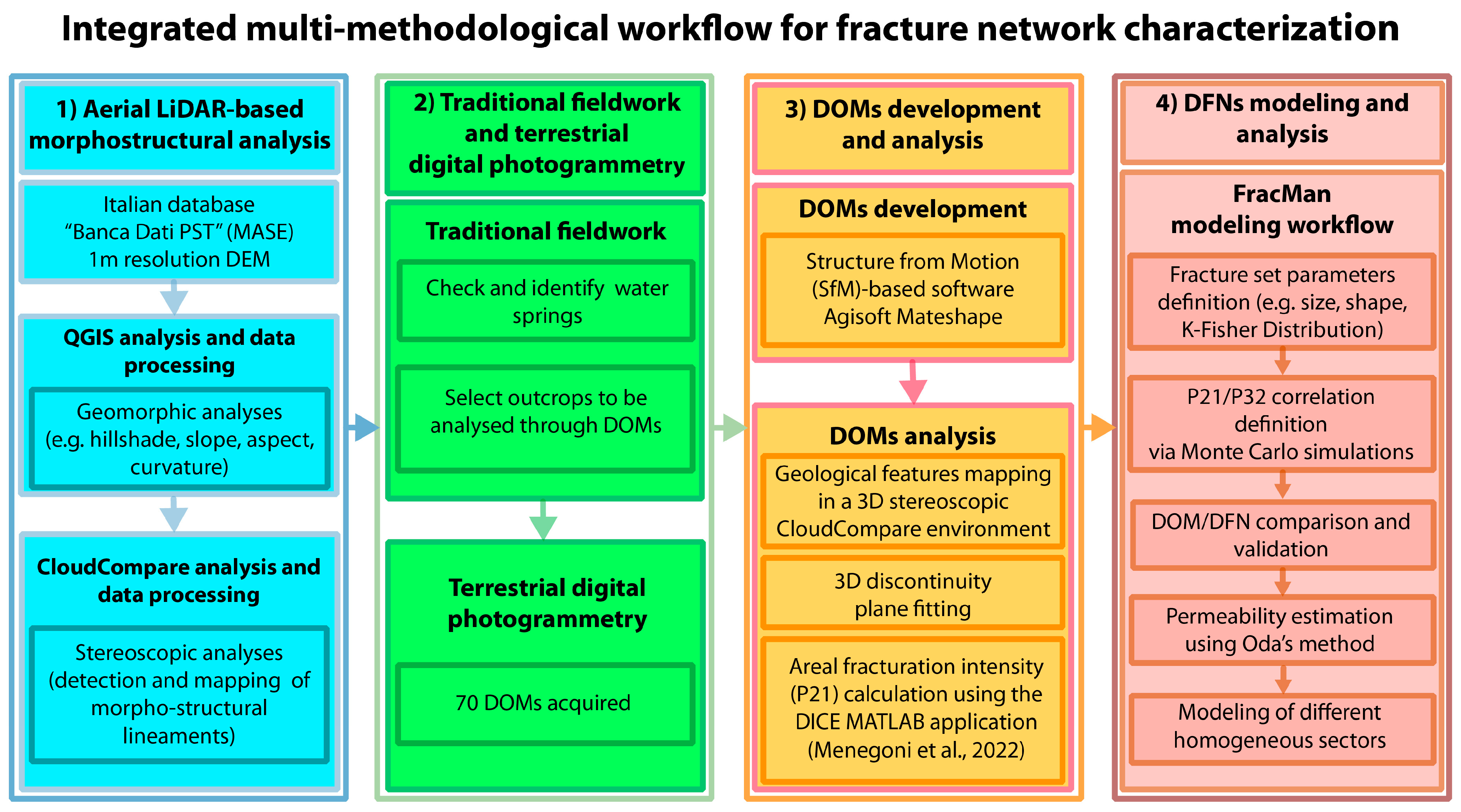
To quantitatively estimate the fracture network parameters and their distributions across the study area, this research is conducted using a multi-methodological approach, combining:

• Aerial LiDAR-based morphostructural analysis to map the main morphostructural lineaments of the study area;
• Traditional fieldwork and terrestrial photogrammetry, to collect major geological information, check and identify water springs together with the local water management authority, and select the best outcrops to be analyzed through DOMs;
• DOM development and analysis, to generate DOMs and quantitatively characterize the fracture network (e.g., dip and dip direction, K-Fisher coefficient, MTL, P21);
• DFN modeling, to predict the preferential fluid flow directions of the analyzed rock mass.

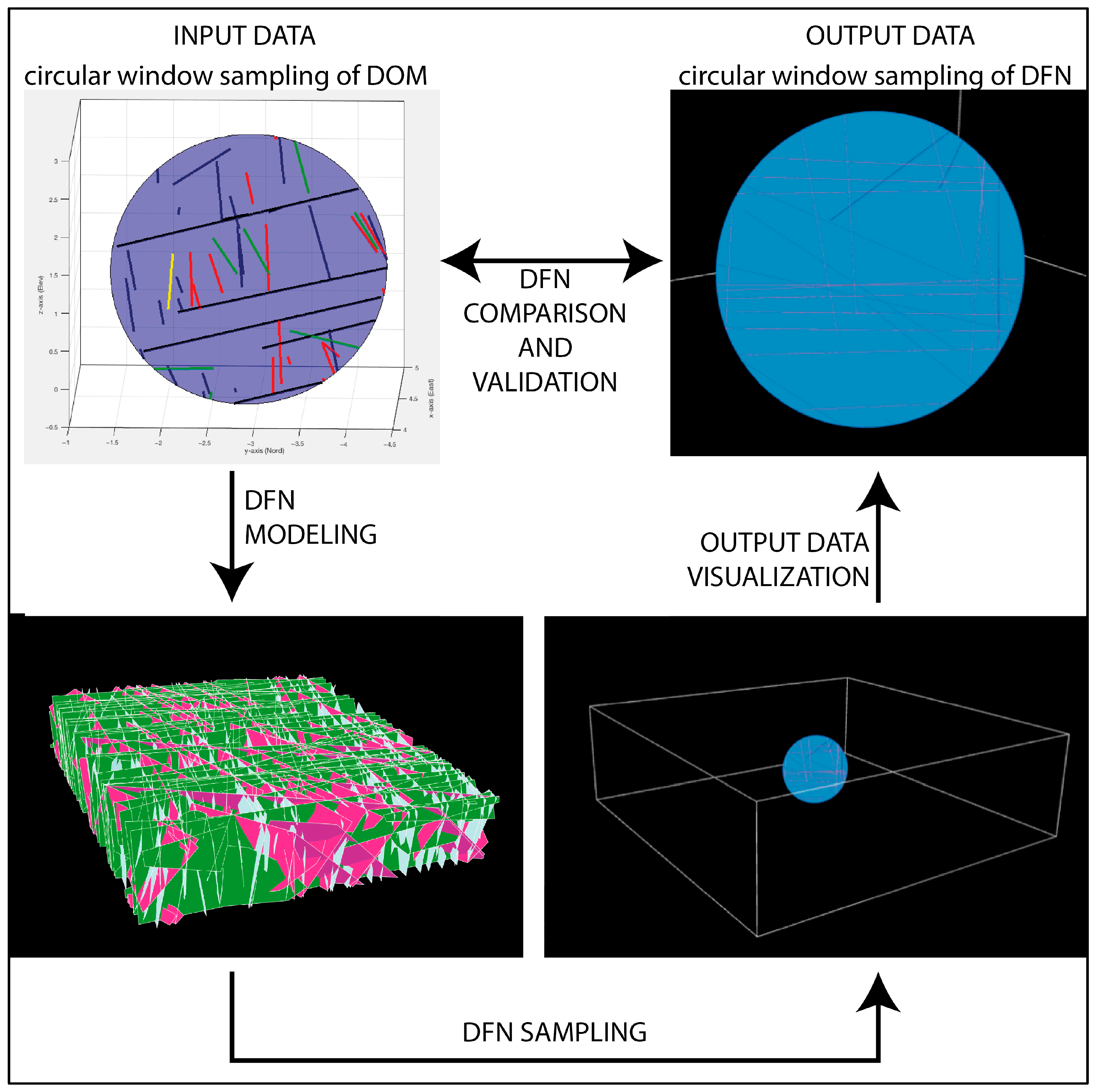
The following subsections describe the methodology, covering the aerial LiDAR-based morphostructural analysis, terrestrial digital photogrammetry, DOM development and analysis, and Discrete Fracture Network modeling. The integrated workflow is depicted in Figure 2.

3.1. Aerial LiDAR-Based Morphostructural Analysis

The aerial LiDAR-based morphostructural analysis was performed using a LiDAR-based Digital Elevation Model (DEM) retrieved from the Italian database “Banca Dati PST” (Ministero dell’Ambiente e della Sicurezza Energetica, MASE; https://sim.mase.gov.it/portalediaccesso/mappe/#/viewer/new/, accessed on 1 May 2026).

This DEM, derived from the aerial LiDAR of the “Piano Straordinario di Telerilevamento” (Ministero dell’Ambiente e della Sicurezza Energetica, MASE), has a resolution of 1 m. It was analyzed using the open-source software QGIS (3.16 “Hannover”)and CloudCompare software (v2.10.2 “Zephyrus”). QGIS allows us to perform several geomorphic analyses (i.e., hillshade, slope, aspect, curvature), while CloudCompare permits us to analyze the DEM in a 3D stereoscopic environment, allowing us to obtain geometric 3D information. The DEM analysis allowed the detection and mapping of the main morphostructural lineaments in the study area.

3.2. Terrestrial Fieldwork and Digital Photogrammetry

Fieldwork was performed in order to collect major geological information, check and identify the water springs together with the local water management authority and select the best outcrops to be acquired with the terrestrial digital photogrammetry approach (Figure 1c).

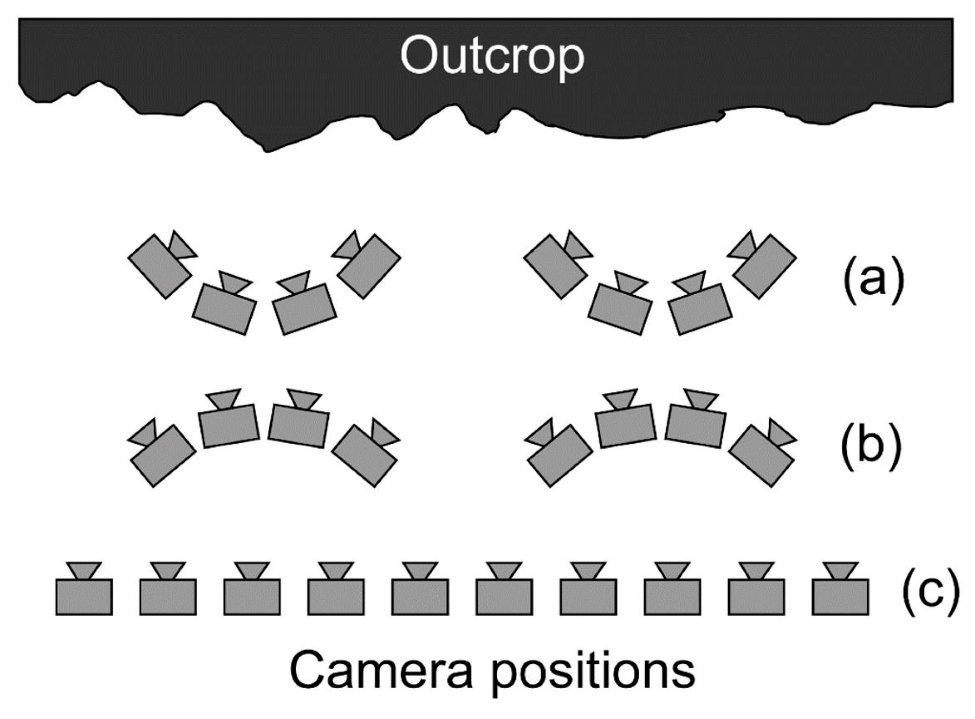
Specifically, we used the digital photogrammetry approach already tested in previous works [14,40,52,53] and a Canon EOS 5D 12.8 Megapixel camera (Canon, Nagasaki, Japan) and a zoom lens, acquiring 70 Digital Outcrop Models (DOMs). For all 70 terrestrial photogrammetric stations (Figure 1), the distance camera-outcrop was 6 m and the focal length 28 mm. The mean ground pixel size of the images, also called ground sampling distances, was 1.8 mm/pixel. Due to the geometry and the small dimension (length < 50 m and height < 10 m) of the analyzed outcrops, the images were acquired using confocal (Figure 3a) and/or strip (Figure 3c) geometries of acquisition.

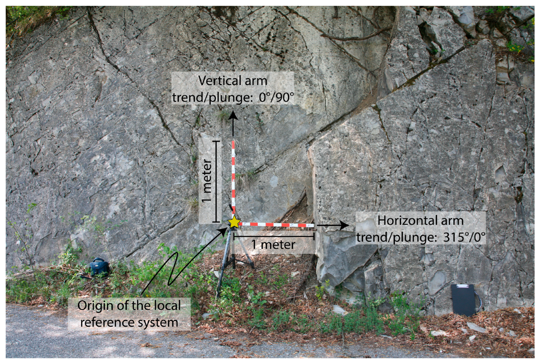
In order to correctly georeference the model in a local coordinate system, we used a photographic scale mounted on a tripod and composed of two arms of 1 m each (Figure 4).

The arms of the photographic scale were settled horizontally and vertically, and then the attitude of the horizontal arms was registered. Whereas the size of the arms is required to scale the DOMs, their attitude is required to correctly orient the DOMs in a local coordinate system in which the origin of the system is settled at the intersection of the arms (see Figure 4 above).

After the photo-acquisition, manual measures of the bedding and fracture were taken using the compass-clinometer. These measures are control measures and, therefore, they are taken into account to assess the validity of the generated DOMs. In general, only clearly exposed surfaces that can be recognized in the photographs have been measured.

3.3. DOM Development and Analysis

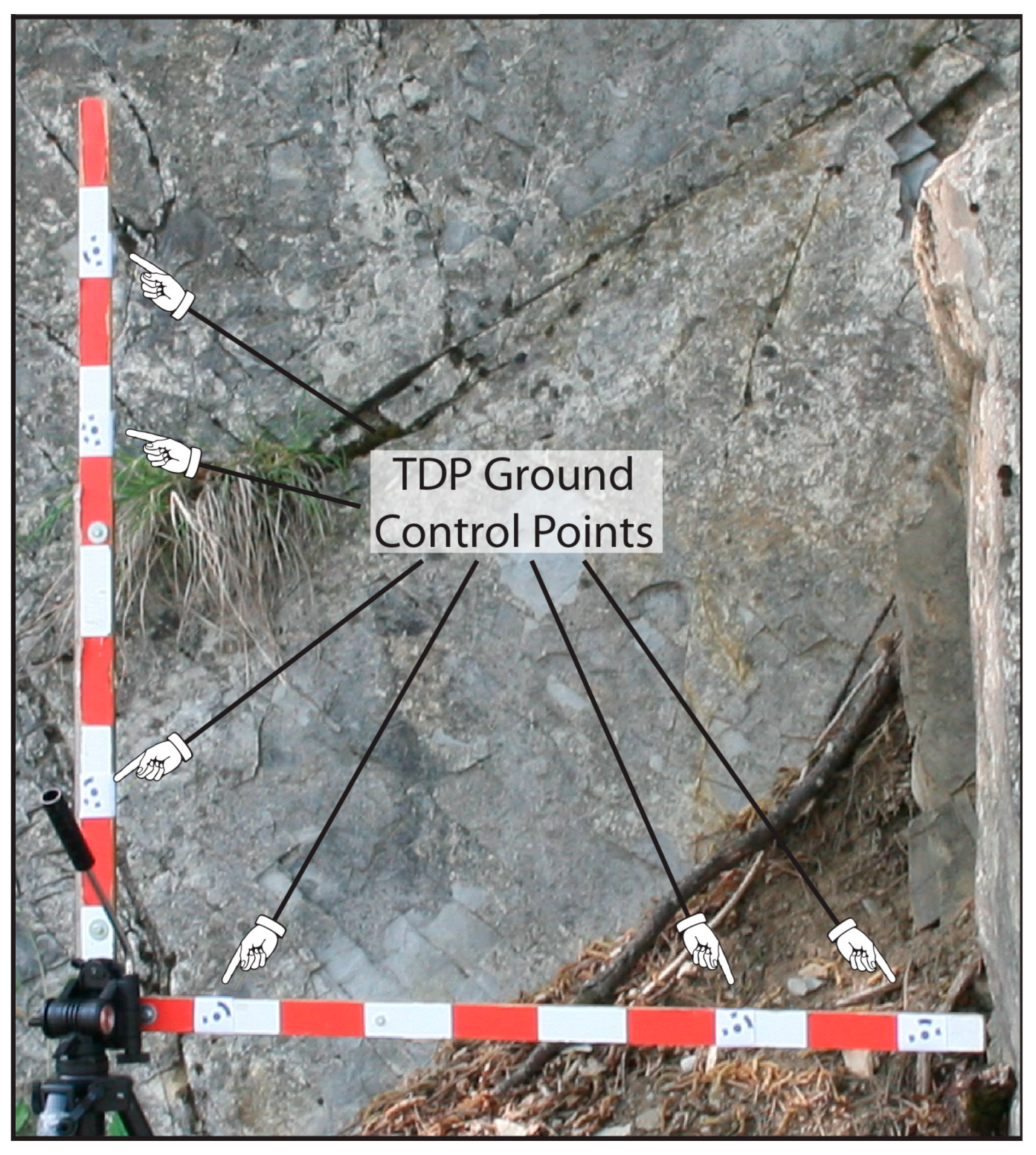
The DOMs were developed using the Structure from Motion (SfM)-based software Agisoft Metashape 2.2.1 (Agisoft LLC, Moscow, Russia). The images were aligned using their full resolution and considering the Ground Control Points (GCPs) present on the photographic scale (example in Figure 5).

Subsequently, the procedures for generating dense clouds were executed using the high-quality setting, accompanied by a mild filtering of the depth map. Following this step, the meshes were generated using the software’s high-quality settings and were textured exclusively with images possessing a quality factor greater than 0.9.

The generated DOMs were then analyzed using the open-source software CloudCompare v.2.9; this allows for DOM analysis and mapping of the geological features in a 3D stereoscopic environment. The stereo-visualization and the structural interpretation and mapping of the DOMs were performed by a Planar SD2220W stereoscopic device, composed of two separate polarized display monitors placed one above the other in a clamshell configuration, with a half-silvered glass plate bisecting the angle between the two displays.

Orientation, dimension, position of bedding and fractures were acquired using CloudCompare and related tools, like: Trace polyline tool, Segment tool, Fit plane tool, and Compass plugin [54]. The calculation of fracture intensity was conducted using the DICE MATLAB© application (Dice V.1.0.) (for full explanation, see [55]). This algorithm enables the computation of linear, area and volumetric fracture intensity (P10, P21 and P32, sensu [56]) in three-dimensional space, taking full advantage of the 3D nature of DOM and digital fracture data.

Among the different options for computing fracture intensity, we decided to analyze P21, since Digital Photogrammetry methods lack information concerning the persistence of fractures beyond outcrop surfaces [54]. The P21 [m⁻¹] is defined as the ratio between the total length of discontinuity traces [m] and the sampling area [m²] [31,56].

3.4. Discrete Fracture Network Modeling and Analysis

To model the DFNs, we used FracMan software (FracMan 8.6) (WSP). The DFN modeling workflow can be summarized as follows:

The first phase is the fracture set parameter definition:

• Fracture orientations, defined as the mean orientation of the fracture sets and their K-Fisher distribution coefficients, that express how tight the clusters of orientations are;
• Fracture size, defined as Mean Trace Length and a log-normal distribution;
• Fracture shape, defined as a rectangle to better represent the mechanical stratigraphy (i.e., stratabound fractures; e.g., [26]);
• Fracture intensity, defined as volumetric intensity value (P32) [56];
• Fracture aperture, defined as a log-normal distribution with a mean value of 0.1 mm [57,58,59].

Note that the definition of the aperture parameter is not based on actual measures and is set as the standard value of FracMan for all the sets. Therefore, the permeability results will be considered relatively and will be mainly affected by differences in fracture intensity and orientation.

The second phase consists of a series of Monte Carlo simulations to define the corrected intensity measure value [25]:

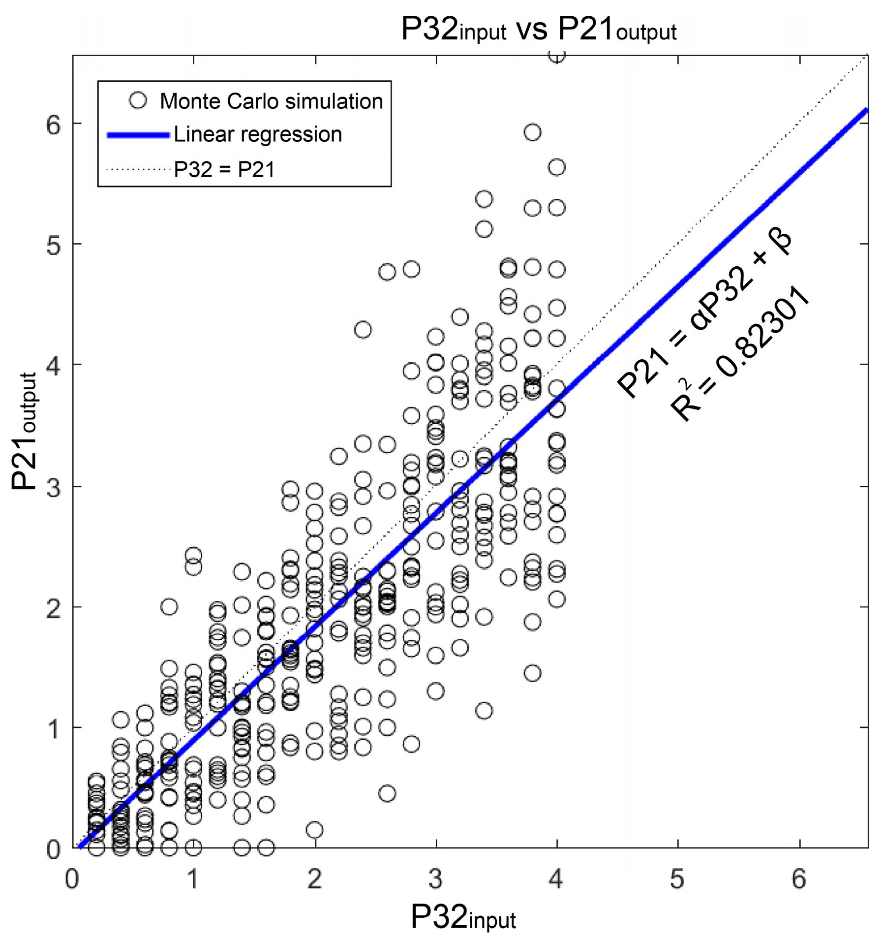
• Due to the impossibility of directly measuring the P32 intensity parameters, several Monte Carlo simulations with different values of P32 (specifically, 10 simulations with a P32 input value ranging from 0.2 to 4 with a step of 0.2 m⁻¹, for each set; 800 simulations) are performed to find the correlation between P32 input and P21 output determined from the DFN model (Figure 6);

2.

When the correlation indexes α and β have been determined, it is possible to infer the correct value of P32 to be used in the modeling from the P21/P10 measured on outcrop/borehole (Figure 7).

3.

The DFN model that best fits the measurements acquired from the outcrop is selected as the representative DFN.

When the DFN is modeled and validated, it is possible to calculate the connectivity of the fracture network and the equivalent permeability of the rock mass volume.

In particular, the permeability is estimated using Oda’s method [60], implemented in the software. Assuming fractures are impermeable in their orthogonal direction, it estimates the permeability according to the fracture orientation in each grid cell.

This procedure of DFN modeling creates homogeneous fracture networks, a case far away from the study area. For this reason, the DFNs were modeled in different homogeneous sectors. These sectors are:

• The zones of normal polarity beds and low fracture intensity;
• The zones of normal polarity beds and high fracture intensity;
• The zones of inverse polarity beds and low fracture intensity;
• The zones of inverse polarity beds and high fracture intensity.

4. Results

4.1. Aerial LiDAR Analysis

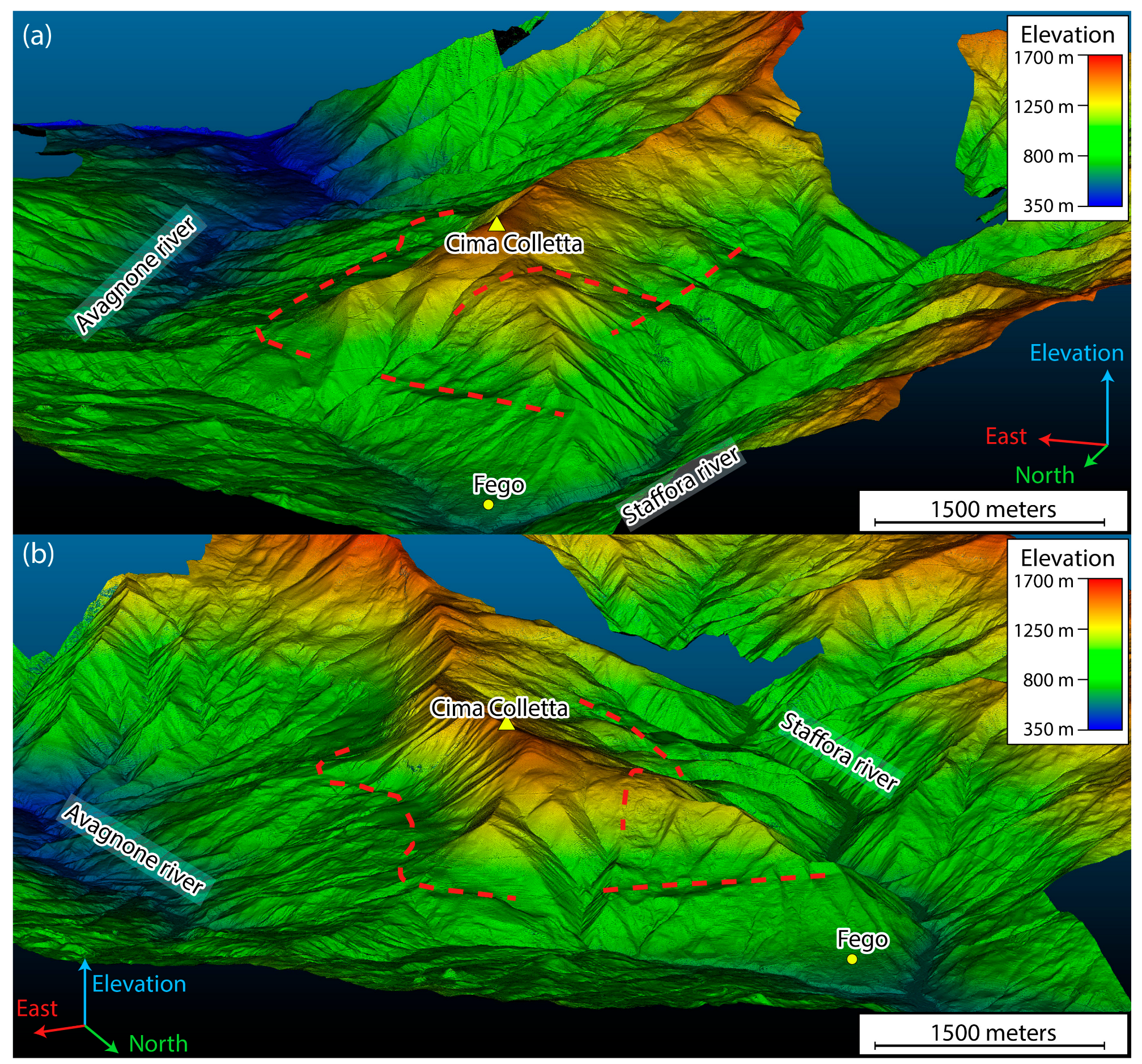
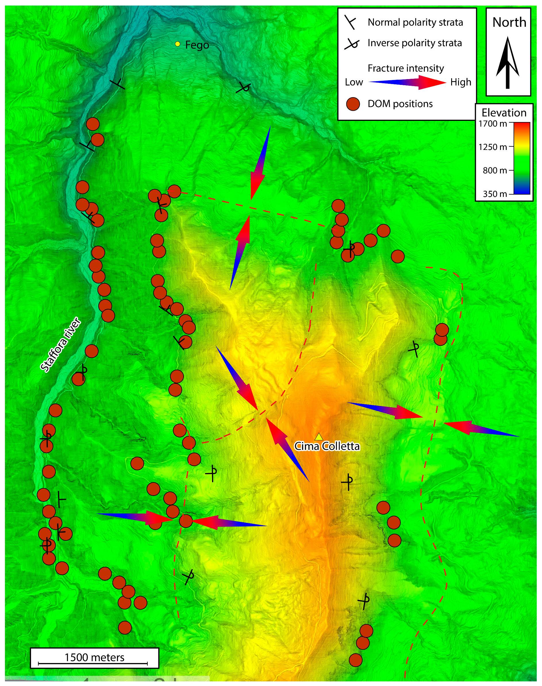
The morphostructural analysis of DEM (Figure 8) allows us to recognize three main counterslopes that delimitate the West, North and East slopes of the mount ‘Cima Colletta’, with an apparent horizontal orientation, and an N-lineament that connects the N with the W-counterslope, with an apparent steeply inclined orientation (Figure 9).

4.2. Fieldwork- and DOM-Based Analysis

The analysis of the sedimentological features of the turbiditic beds indicates the presence of normal and inverse polarity strata. The lineaments detected on the DEM seem to divide sectors of different strata polarity (Figure 9). Moreover, the quantitative analyses of fracture intensity performed respectively during the geological field survey and the 3D DOM analysis show that as one gets closer to the detected lineaments, the fracture intensity increases significantly.

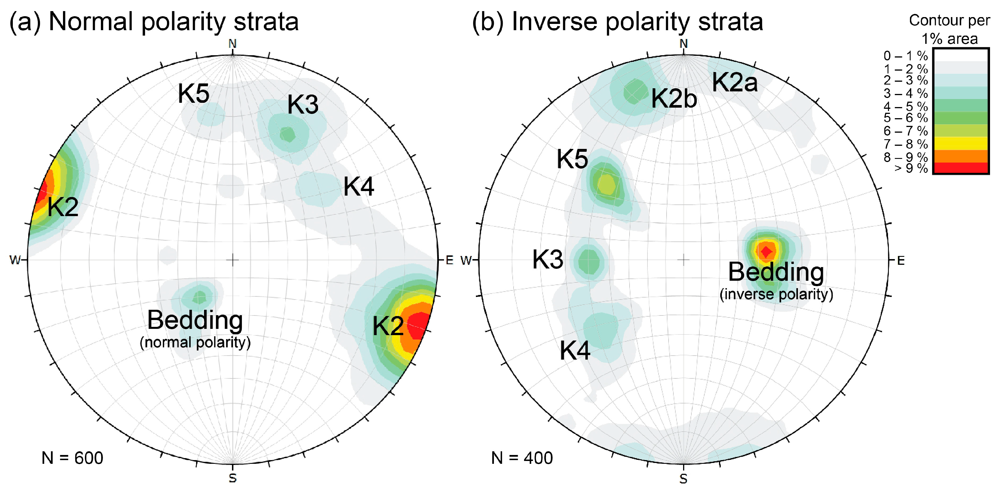
The analyses of DOMs performed in the different structural sectors (Figure 1c and Figure 9) highlight that the fracture sets maintain constant geometric relationships to bedding both in normal and inverse polarity strata (Figure 10).

This relation between fractures and bedding was already detected by the structural analysis of [61], performed on the Monte Antola Fm. cropping out about 6 km SW of the study area, and interpreted as a specific fracture orientation pattern related to folding: K2 possibly represents the longitudinal/radial/hinge-parallel fracture set; K3 the cross/extensional/hinge-orthogonal fracture set; and K4 and K5 the conjugate shear fractures.

Except for the fracture set orientation, DOMs also allowed for the acquisition of all the fracture parameters required for the DFN models, i.e., mean orientation of fracture sets, orientation dispersion of fracture sets (K-Fisher’s coefficient), fracture intensity and fracture mean trace length. These parameters are calculated considering the 3D nature of the fracture and sampling the properties using 3D sampling techniques (i.e., 3D circular scan plane of DICE).

Table 1. Fracture parameters obtained for DOMs with different polarities in low-intensity areas. Only the parameters required by DFN modeling are reported.

Fracture Parameters	Normal Polarity Strata				Inverse Polarity Strata
	K2	K3	K4	K5	K2	K3	K4	K5
Dip (°)	88	70	56	71	83	49	55	54
Dip Direction (°North)	291	203	232	172	175	88	49	134
K-Fisher coefficient	74.85	68.87	71.29	120.57	92.37	189.2	69.11	104.42
P21 (m−1)	4.06	12.57	10.12	3.62	2.48	14.10	13.09	2.48
Mean trace length (m)	0.63	0.72	1.90	0.39	1.15	5.06	4.17	1.12

and

Table 2. Fracture parameters obtained for DOMs with different polarities in ‘high’ fracture intensity. Only the parameters required by DFN modeling are reported.

Fracture Parameters	Normal Polarity Strata				Inverse Polarity Strata
	K2	K3	K4	K5	K2	K3	K4	K5
Dip (°)	89	72	58	70	87	48	53	60
Dip Direction (°North)	287	194	225	165	171	85	50	136
K-Fisher coefficient	83.65	74.68	71.90	100.34	70.36	133.12	80.91	95.13
P21 (m−1)	10.45	18.79	13.65	12.10	8.67	21.56	16.34	14.62
Mean trace length (m)	0.35	0.45	0.80	0.42	0.92	1.22	0.95	1.03

show the mean comprehensive fracture parameters retrieved from the full DOM dataset, reporting low- and high-intensity areas for both outcrops with normal and inverse polarities. These outcrop data will be later used for DFN modeling.

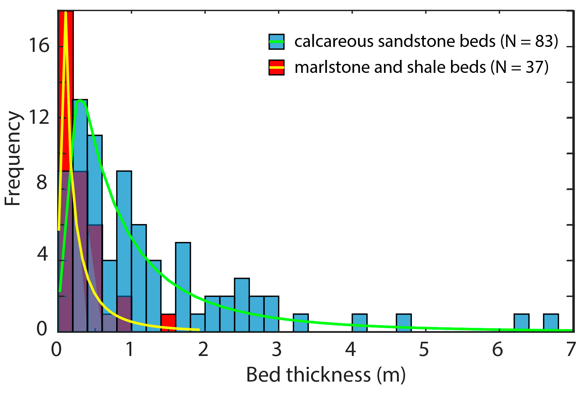
Along the analyzed structural stations, bedding appears highly persistent, with no pinch-out and/or abrupt lateral termination of strata, and nearly planar, with no evident folds but only small-scale undulations (maximum amplitude 5 cm and minimum wavelength of 20 cm). For this reason, for bedding, we considered constant orientation and a very high persistence, defining a fracture size higher than the DFN simulation volume size (i.e., >10 m). Moreover, using the P10: scanline sampling of DICE, the thickness of 120 beds was measured, showing a log-normal distribution with a mean thickness of about 30 cm (Figure 11).

4.3. DFN Modeling

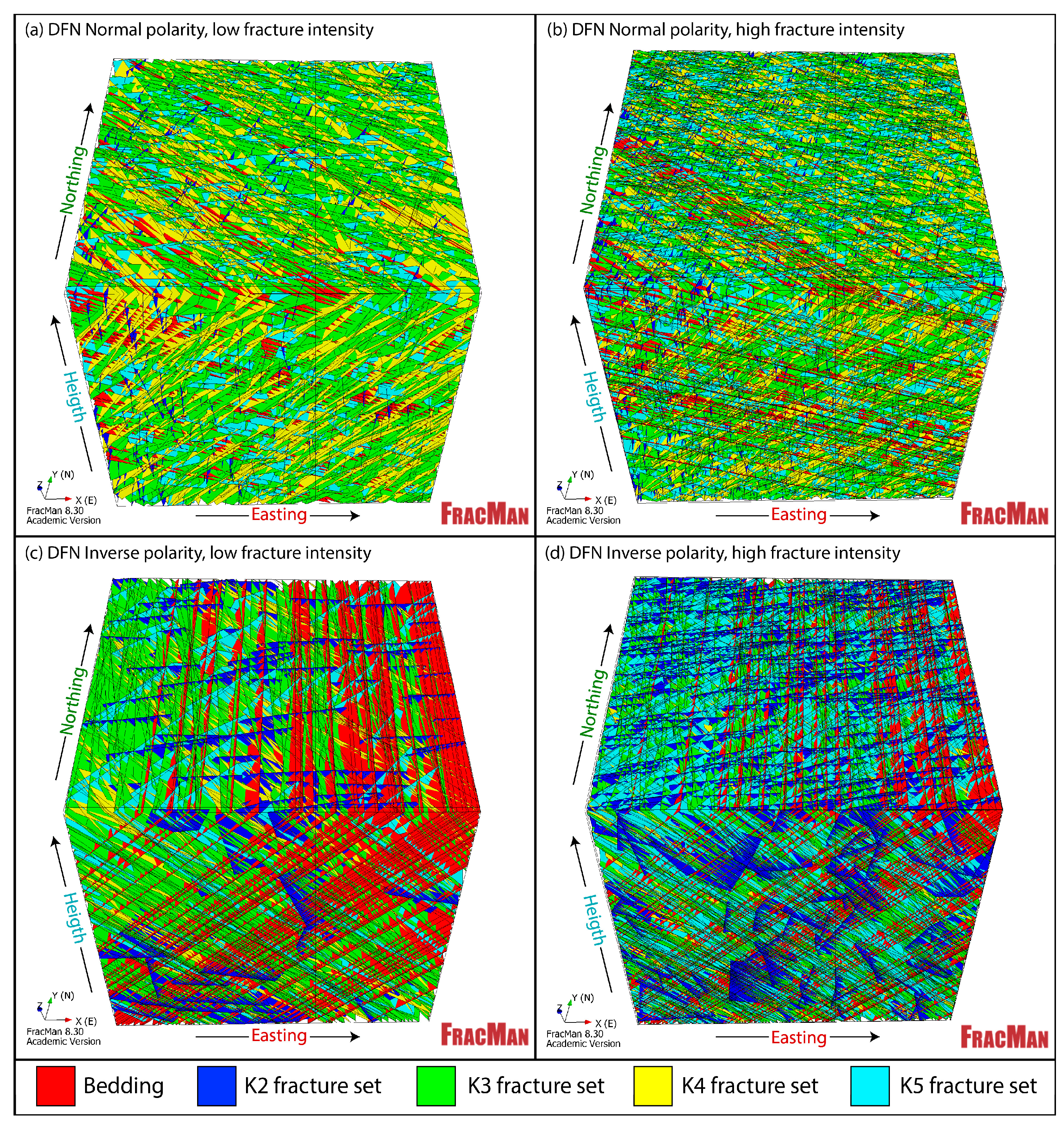
The DFN modeling and analysis were performed in a volume of 10 m × 10 m × 10 m (Figure 12) in order to decrease the amount of computational time and not overload the computer CPU.

Due to the mean trace length of the fractures, generally lower than 1 m, the settled volume does not affect the results negatively with truncation effect.

When fed by constant values and statistical distribution, as in our case, DFN modeling creates ‘statistically homogeneous’ fracture networks. Since we do not aim to build a reservoir-scale fracture network, but we want to highlight the differences between the different “structural sectors”, DFN models have been performed for normal and inverse polarities and low and high fracture intensities (Figure 10). For the same reason, an analysis of the representative elementary volume (REV) has not been performed since we do not need to build huge models and extract precise and accurate permeability parameters (as previously mentioned, we will consider the relative differences in permeability). The α and β values used for the correction of the P32 input values of the DFN models are 0.88 and −0.05, respectively. To assess the validity of the DFN models, the same circular windows used to extrapolate the fracture parameters onto the 3D DOM were used on the DFN models (as shown in Figure 6). This comparison shows similar results and, therefore, indicates a good validity of the models (example in

Table 3. Comparison between fracture parameters sampled on the DOM and on the DFN for low fracture intensity areas.

		Normal Polarity Strata				Inverse Polarity Strata
		K2	K3	K4	K5	K2	K3	K4	K5
Sampled on DOM	P21 (m−1)	4.06	12.57	10.12	3.62	2.48	14.10	13.09	2.48
	MTL (m)	0.63	0.72	1.90	0.39	1.15	5.06	4.17	1.12
Sampled on DFN	P21 (m−1)	4.15	12.30	10.10	3.02	2.34	13.59	13.60	2.28
	MTL (m)	0.62	0.64	1.82	0.50	1.24	4.87	5.28	1.43

and

Table 4. Comparison between fracture parameters sampled on DOM and on DFN for high fracture intensity areas.

		Normal Polarity Strata				Inverse Polarity Strata
		K2	K3	K4	K5	K2	K3	K4	K5
Sampled on DOM	P21 (m−1)	10.45	18.79	13.65	12.10	8.67	21.56	16.34	14.62
	MTL (m)	0.35	0.45	0.80	0.42	0.92	1.22	0.95	1.03
Sampled on DFN	P21 (m−1)	10.23	18.54	11.01	12.01	9.09	21.32	16.67	12.89
	MTL (m)	0.24	0.76	0.83	0.44	1.11	1.51	1.06	1.38

).

Moreover, using the FracMan toolbox Cluster Analysis, we calculated the pseudo connectivity of fractures (i.e., clustering). The analysis shows that for each sector, all the fractures are connected in a single cluster (i.e., 100% of fractures are connected).

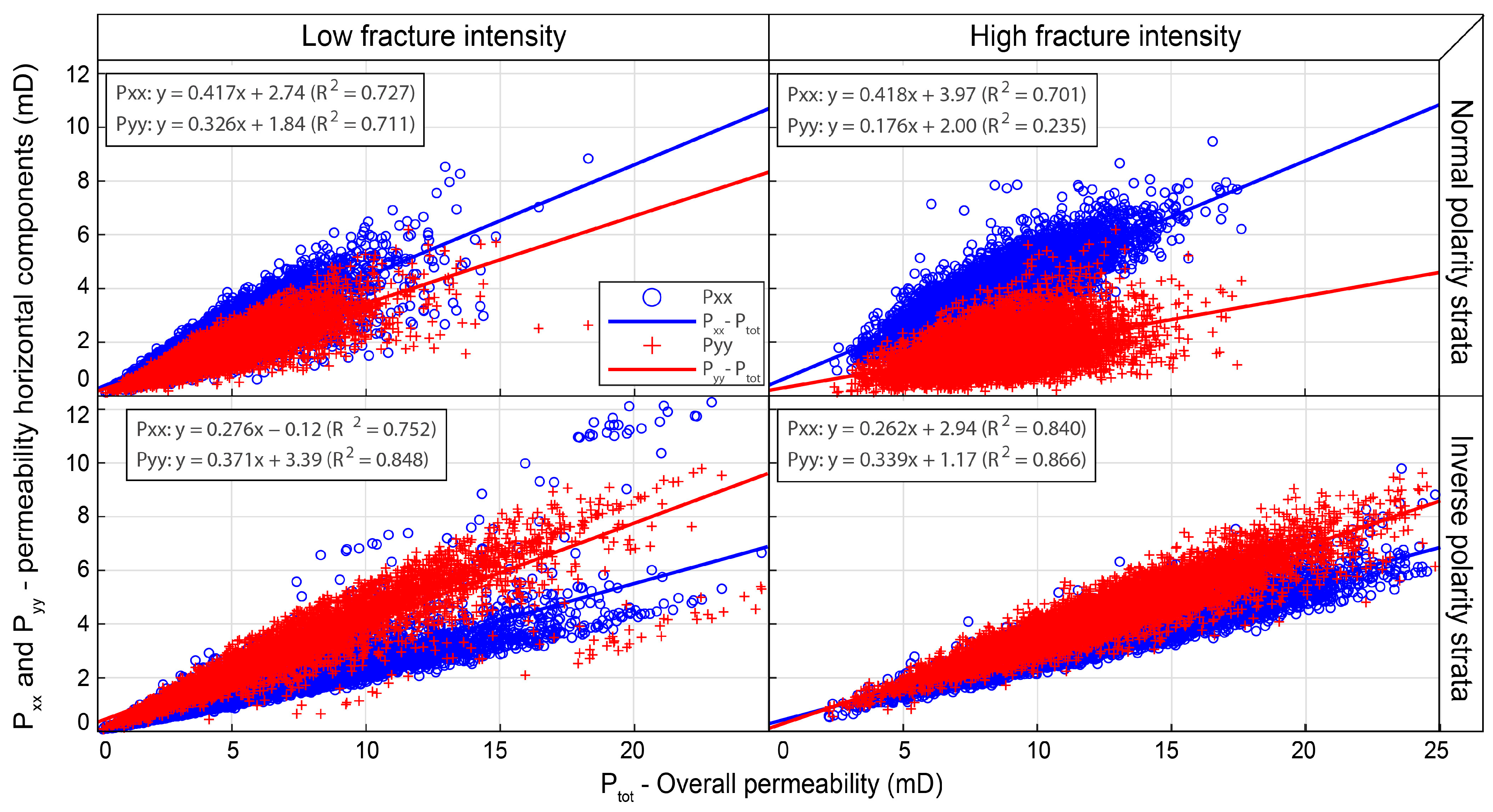
DFN-related permeability analysis was conducted by decomposing the permeability vectors in their xx and yy components in order to understand the principal direction of flow. This decomposition suggests that in both normal and inverse polarity strata, the higher permeability component is sub-parallel to the K3 direction, Pxx and Pyy, respectively, for normal and inverse polarity strata (Figure 13). Notwithstanding, the difference between them is small and therefore cannot strongly influence the fluid flow direction.

From the comparison of areas with low and high fracture intensity (Figure 13 and

Table 5. Mean value of the horizontal permeability components Pxx and Pyy for the normal (NP) and inverse polarity strata (IP), and for low (LP) and high fracture intensity (HP).

		Pxx (mD)	Pyy (mD)
NP	LI	2.2	1.7
	HI	3.9	2.6
IP	LI	2.7	4.4
	HI	3.6	4.5

), it is clearly visible that in high-intensity areas, the permeability values can be from 2% to 79% higher than the values of low-intensity areas and, therefore, could strongly influence the fluid circulation in the rock mass.

5. Discussion

The results presented in this paper are based on a combination of multiple approaches based on aerial LiDAR DEM remote sensing morphometric analysis, fieldwork observations, Digital Outcrop Model-based fracture analysis and DFN modeling. Through the DEM-based remote sensing analysis, we were able to detect and localize the four main morphostructural lineaments in the study area (Figure 8): three lineaments with an apparent horizontal attitude that delimit the W, N and E slopes of the mount ‘Cima Colletta’, and an NNE-SSW trending lineament with an apparent steeply inclined attitude.

The field-survey and DOM analysis suggests a correlation between the main lineaments in the study area and deformation structures like fold axial planes and faults, as already described in nearby areas [61]. This interpretation is supported considering that these lineaments separate different structural sectors where the Monte Antola Fm. has different bed polarity and are associated with an increase in the fracture intensity (Figure 9). During fieldwork, we were not able to clearly observe evidence of these structures due to the extensive debris and vegetation coverage. This is possibly because these areas are characterized by a very intense deformation that favors the development of soil and the growth of vegetation.

The analysis of the DOM, developed using terrestrial digital photogrammetry, shows the presence of four fracture sets clearly visible along the entire study area (Figure 10). These four sets keep the same mutual angular relationships with bedding in all the different structural positions. Thanks to the use of the DICE, it was possible to characterize the areal fracture intensity (P21) directly on the 3D Digital Outcrop Model. This novel technique allowed us to quantitatively describe fractures and, therefore, to calculate the parameters required for DFN modeling (Figure 12). Using this DOM-based 3D approach, we were able to avoid the errors that often affect the traditional field-based approach and the 2D image sampling technique (e.g., length and orientation biases). Note that, as shown in [55], the DOMs are 2.5D surfaces (2D surfaces in a 3D space) and, therefore, some limitation on the 3D geometrical definition of fractures may still persist.

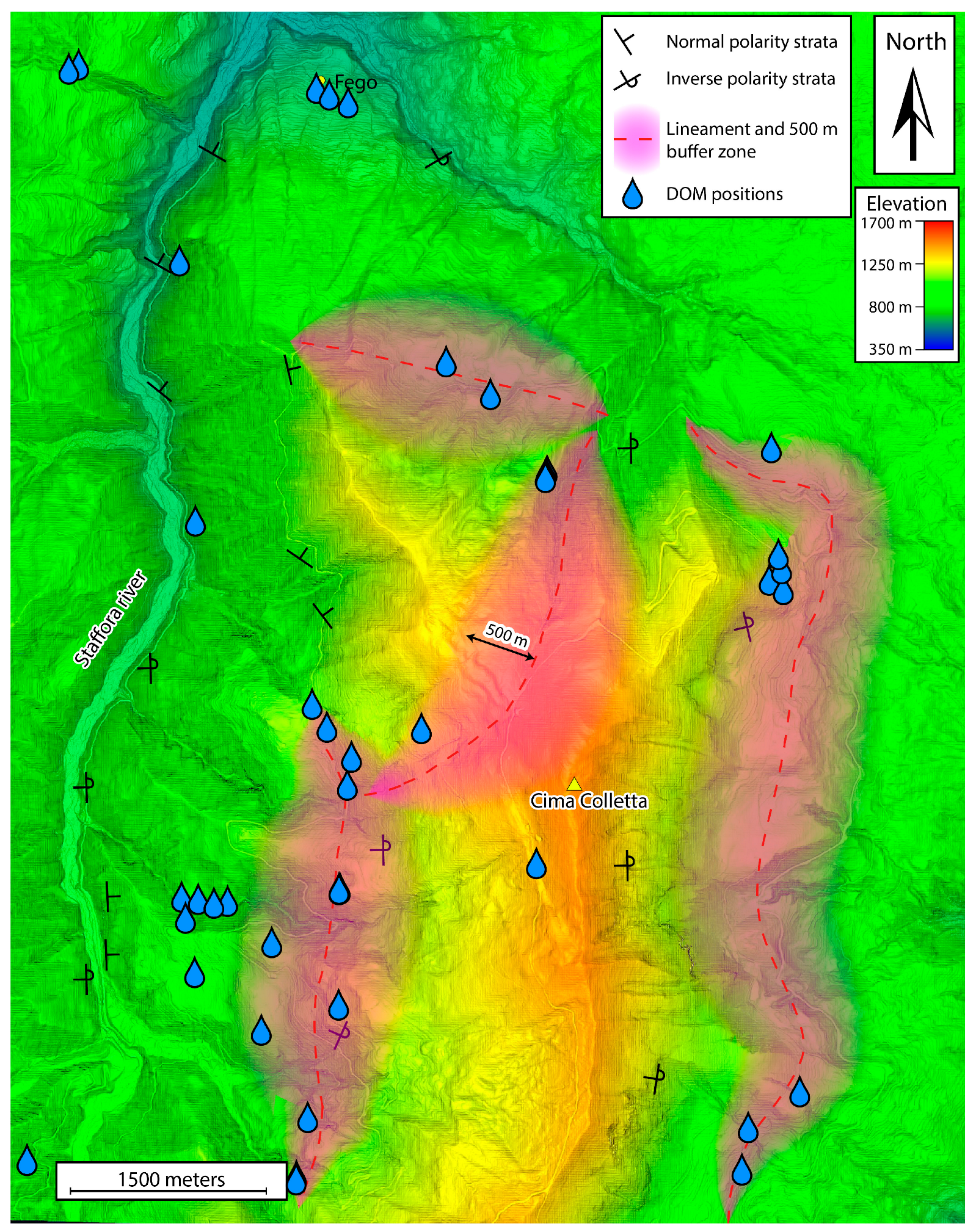
The developed DFN models show good validity because the comparison of the data acquired using a 3D circular window sampling onto the DOM and those acquired using the same 3D circular window onto the DFN is pretty similar (Table 3 and Table 4). The DFN properties of all the different structural sectors permit us to predict a fluid flow mainly concentrated along the K3 fracture set direction (Figure 13). In particular, due to the high fracture intensity, the DFN suggests a major fluid circulation in the lineament area, where the horizontal permeability components parallel to K3 increase from 3% (inverse polarity strata) to 79% (normal polarity strata) (Table 5). The positions of the water springs allow us to check and validate the DFN permeability results; water springs seem to be aligned along a preferential direction in the surroundings of the main morphostructural lineaments (Figure 14).

In particular, most of the water springs seem to be located in a buffer zone of about 500 m with respect to the mapped lineaments. This suggests that these zones can be characterized by a higher fracture intensity and, therefore, drive the fluid flow. Most probably, these areas correspond to fold-hinges characterized by a high abundance of hinge parallel fractures (K3).

Despite these considerations, our DFN simulations are affected by the following main limitations:

• Aperture has been considered constant for all the sets and structural sectors, without differentiating fractures that can have a different origin (e.g., mode-I, II and III) and evolution (impacting on roughness and terminations);
• Major structural elements such as incipient faults or fracture corridors have not been considered;
• Oda’s assumptions (e.g., impermeable matrix, parallel-plate flow, full intra-cell connectivity, and no roughness/tortuosity) may not perfectly fit the fracture formation, in which partially cemented fractures can be present;
• The parametric Monte Carlo framework requires distributional assumptions at every step; each contributes to increasing uncertainties [62].

For these reasons, the permeability values retrieved from DFN and Oda’s permeability simulations should be considered relatively and not as precise and accurate values that can populate a reservoir permeability model. Despite that, our analysis shows that with these limitations, our “simplified” model agrees with the observation about water springs. Further studies based on the accurate set-by-set characterization of fracture aperture, roughness and termination, the definition of major structural elements outcropping in the area, and the use of an alternative framework to Oda’s and Monte Carlo simulations (e.g., FracGen; [62]) will allow us to build a more realistic and accurate quantitative model of the reservoir.

6. Conclusions

In this paper, we present an integrated workflow offering a robust methodology to enhance the DFN model using DOM fracture measurements. Using a combination of traditional fieldwork and DP, it was possible to obtain quantitative information on fracture networks, defining the main fracture sets affecting the Monte Antola Formation in the Upper Staffora Valley area (Northern Apennines, Italy). A proper characterization of the fracture network is crucial, as fractures significantly influence the permeability and fluid flow circulation in the subsurface. This has significant implications for the characterization of various types of fractured reservoirs, such as those related to water supply, hydrocarbons, geothermal energy, and carbon capture and storage. For this reason, the accurate development of DFN models is crucial to predict reservoir behavior. The main results are listed as follows:

• Through the use of DOMs, we were able to obtain high-accuracy and high-resolution 3D fracture measurements and, therefore, accurately quantify the fracture parameters required to model the DFNs.
• DFN models allowed estimation of permeability tensors, suggesting that fluid flow is mainly concentrated along the fracture set K3 and the lineament zones.
• Water springs tend to be located in correspondence with the main morphostructural lineaments detected during the analysis of the aerial LiDAR DEM, suggesting an influence on fluid flow of fractures at a larger scale.

In conclusion, we have shown that the DOM and DFN model can be effective for the analysis of fractured reservoirs, giving the possibility to perform reliable predictions on fluid flow. We established a link between the fracture set observed along outcrop and subsurface fluid flow. Despite that, to fully understand the geohydrological system, further studies are required in order to reconstruct the 3D subsurface geological model, including the main deformation structures.

References

1. Baronetti, A.; Dubreuil, V.; Provenzale, A.; Fratianni, S. Future droughts in northern Italy: High-resolution projections using EURO-CORDEX and MED-CORDEX ensembles. Clim. Chang. 2022, 172, 22. [Google Scholar] [CrossRef] [Scilit]
2. Boyko, O.; Reggiani, P.; Todini, E. Post-processing climate projections of precipitation for the Po river basin: Will Italy’s North become water-constrained? Hydrol. Res. 2022, 53, 1414–1427. [Google Scholar] [CrossRef] [Scilit]
3. Koehler, J.; Dietz, A.J.; Zellner, P.; Baumhoer, C.A.; Dirscherl, M.; Cattani, L.; Kuenzer, C.; Vlahović, Ž.; Alasawedah, M.H.; Mayer, K.; et al. Drought in Northern Italy: Long Earth Observation Time Series Reveal Snow Line Elevation to Be Several Hundred Meters Above Long-Term Average in 2022. Remote Sens. 2022, 14, 6091. [Google Scholar] [CrossRef] [Scilit]
4. Colombo, N.; Guyennon, N.; Valt, M.; Salerno, F.; Godone, D.; Cianfarra, P.; Romano, E.; Freppaz, M.; Maugeri, M.; Manara, V.; et al. Unprecedented snow-drought conditions in the Italian Alps during the early 2020s. Environ. Res. Lett. 2023, 18, 074014. [Google Scholar] [CrossRef] [Scilit]
5. Zimmerman, R.; Main, I. Chapter 7 Hydromechanical Behavior of Fractured Rocks. Int. Geophys. 2004, 89, 363–421. [Google Scholar] [CrossRef] [Scilit]
6. Park, R.G. Foundation of Structural Geology; Taylor & Francis: London, UK, 2013; pp. 1–202. [Google Scholar] [CrossRef] [Scilit]
7. Lei, Q.; Latham, J.-P.; Tsang, C.F. The use of discrete fracture networks for modelling coupled geomechanical and hydrological behaviour of fractured rocks. Comput. Geotech. 2017, 85, 151–176. [Google Scholar] [CrossRef] [Scilit]
8. Han, S.; Wang, G.; Li, M. A trace map comparison algorithm for the discrete fracture network models of rock masses. Comput. Geosci. 2018, 115, 31–41. [Google Scholar] [CrossRef] [Scilit]
9. Finkbeiner, T.; Barton, C.A.; Zoback, M.D. Relationships among in-situ stress, fractures and faults, and fluid flow: Monterey Formation, Santa Maria Basin, California. AAPG Bull. 1997, 81, 1975–1999. [Google Scholar] [CrossRef] [Scilit]
10. de La Vaissière, R.; Armand, G.; Talandier, J. Gas and water flow in an excavation-induced fracture network around an underground drift: A case study for a radioactive waste repository in clay rock. J. Hydrol. 2015, 521, 141–156. [Google Scholar] [CrossRef] [Scilit]
11. Junkin, W.; Janeczek, D.; Bastola, S.; Wang, X.; Cai, M.; Fava, L.; Sykes, E.; Munier, R.; Srivastava, R.M. Discrete fracture network generation for the Äspö TAS08 tunnel using MoFrac. In Proceedings of the 51st US Rock Mechanics/Geomechanics Symposium; ARMA: Prague, Czech Republic, 2017; Volume 2, pp. 1247–1256. [Google Scholar]
12. McNamara, D.D.; Milicich, S.D.; Massiot, C.; Villamor, P.; McLean, K.; Sépulveda, F.; Ries, W.F. Tectonic controls on Taupo Volcanic Zone geothermal expression: Insights from Te Mihi, Wairakei geothermal field. Tectonics 2019, 38, 3011–3033. [Google Scholar] [CrossRef] [Scilit]
13. Tóth, E.; Hrabovszki, E.; Schubert, F.; Tóth, T.M. Discrete fracture network (DFN) modelling of a high-level radioactive waste repository host rock and the effects on its hydrogeological behaviour. J. Struct. Geol. 2022, 156, 104556. [Google Scholar] [CrossRef] [Scilit]
14. Fedorik, J.; Delaunay, A.; Losi, G.; Panara, Y.; Menegoni, N.; Afifi, A.M.; Arkadakskiy, S.; Al Malallah, M.; Oelkers, E.; Gislason, S.R.; et al. Structure and fracture characterization of the Jizan group: Implications for subsurface CO2 basalt mineralization. Front. Earth Sci. 2023, 10, 946532. [Google Scholar] [CrossRef] [Scilit]
15. Massiot, C.; Milicich, S.D.; Sepulveda, F.; Sophy, M.J.; Lawrence, M.J.F.; Griffin, A.G.; Rickman, M.; Carson, L.B.; Rosenberg, M.; Simpson, M. Highlights of Borehole Imaging, Tauhara Geothermal Field Drilling, New Zealand. In Proceedings of the World Geothermal Congress, Beijing, China, 17–21 April 2023; International Geothermal Association (IGA): Hague, The Netherlands, 2023. [Google Scholar]
16. Rosenqvist, M.P.; Meakins, M.W.; Planke, S.; Millett, J.M.; Kjøll, H.J.; Voigt, M.J.; Jamtveit, B. Reservoir properties and reactivity of the Faroe Islands Basalt Group: Investigating the potential for CO2 storage in the North Atlantic Igneous Province. Int. J. Greenh. Gas Control 2023, 123, 103838. [Google Scholar] [CrossRef] [Scilit]
17. Zoback, M.D. Reservoir Geomechanics; Cambridge University Press: New York, NY, USA, 2007; ISBN 978-0-521-77069-9. [Google Scholar]
18. Faulkner, D.R.; Jackson, C.A.L.; Lunn, R.J.; Schlische, R.W.; Shipton, Z.K.; Wibberley, C.A.J.; Withjack, M.O. A review of recent developments concerning the structure, mechanics and fluid flow properties of fault zones. J. Struct. Geol. 2010, 32, 1557–1575. [Google Scholar] [CrossRef] [Scilit]
19. Vidal, J.; Genter, A. Overview of naturally permeable fractured reservoirs in the central and southern Upper Rhine Graben: Insights from geothermal wells. Geothermics 2018, 74, 57–73. [Google Scholar] [CrossRef] [Scilit]
20. Inama, R.; Menegoni, N.; Perotti, C. Syndepositional fractures and architecture of the lastoni di formin carbonate platform: Insights from virtual outcrop models and field studies. Mar. Pet. Geol. 2020, 121, 104606. [Google Scholar] [CrossRef] [Scilit]
21. Cardona, A.; Finkbeiner, T.; Santamarina, J.C. Natural rock fractures: From aperture to fluid flow. Rock Mech. Rock Eng. 2021, 54, 5827–5844. [Google Scholar] [CrossRef] [Scilit]
22. Kissling, W.M.; Massiot, C. Modelling of flow through naturally fractured geothermal reservoirs, Taupō Volcanic Zone, New Zealand. Geotherm. Energy 2023, 11, 20. [Google Scholar] [CrossRef] [Scilit]
23. Kharrat, R.; Ott, H. A Comprehensive Review of Fracture Characterization and Its Impact on Oil Production in Naturally Fractured Reservoirs. Energies 2023, 16, 3437. [Google Scholar] [CrossRef] [Scilit]
24. Hu, L. A review of mechanical mechanism and prediction of natural fracture in shale. Arab. J. Geosci. 2022, 15, 474. [Google Scholar] [CrossRef] [Scilit]
25. Elmo, D.; Rogers, S.; Stead, D.; Eberhardt, E. Discrete fracture network approach to characterise rock mass fragmentation and implications for geomechanical upscaling. Min. Technol. 2014, 123, 149–161. [Google Scholar] [CrossRef] [Scilit]
26. Zambrano, M.; Tondi, E.; Korneva, I.; Panza, E.; Agosta, F.; Janiseck, J.M.; Giorgioni, M. Fracture properties analysis and discrete fracture network modelling of faulted tight limestones, Murge Plateau, Italy. Ital. J. Geosci. 2016, 135, 55–67. [Google Scholar] [CrossRef] [Scilit]
27. Cacciari, P.P.; Futai, M.M. Modeling a shallow rock tunnel using terrestrial laser scanning and discrete fracture networks. Rock Mech. Rock Eng. 2017, 50, 1217–1242. [Google Scholar] [CrossRef] [Scilit]
28. Rogers, S.F.; Bewick, R.P.; Brzovic, A.; Gaudreau, D. Integrating photogrammetry and discrete fracture network modelling for improved conditional simulation of underground wedge stability. In Proceedings of the Eighth International Conference on Deep and High Stress Mining; Wesswloo, J., Ed.; Australian Centre for Geomechanics: Perth, Australia, 2017; pp. 599–610. [Google Scholar] [CrossRef] [Scilit]
29. Monsalve, J.J.; Baggett, J.; Bishop, R.; Ripepi, N. Application of laser scanning for rock mass characterization and discrete fracture network generation in an underground limestone mine. Int. J. Min. Sci. Technol. 2019, 29, 131–137. [Google Scholar] [CrossRef] [Scilit]
30. Fang, H.; Zhu, J.; Qiu, J.; Su, Y.; Xia, D. Laminar and turbulent groundwater flows in confined two- and three-dimensional discrete fracture networks. Eng. Geol. 2022, 308, 106824. [Google Scholar] [CrossRef] [Scilit]
31. Dershowitz, W.; Einstein, H. Characterizing rock joint geometry with joint system models. Rock Mech. Rock Eng. 1988, 21, 21–51. [Google Scholar] [CrossRef] [Scilit]
32. Rogers, S.; Moffitt, K. Probabilistic slope and tunnel block stability analysis using realistic fracture network models. In ARMA US Rock Mechanics/Geomechanics Symposium; ARMA: Prague, Czech Republic, 2006. [Google Scholar]
33. Menegoni, N.; Fedorik, J.; Panara, Y.; Berno, D.; Addassi, M.; Omar, A.; Finkbeiner, T.; Oelkers, E.; Afifi, A.; Hoteit, H.; et al. Subsurface fracture network characterization for a CO2 basalt mineralization target: New insight on fluid flow from wellbore logs for the Jizan Group. Geoenergy 2025, 3, geoenergy2024-037. [Google Scholar] [CrossRef] [Scilit]
34. Fulcher, S.A.; Jordan, T.E.; Laubach, S.E.; Elliott, S.J.; Herrera, V.N. Improving borehole fracture characterization using oriented sidewall cores for geothermal assessment—An example in central New York State USA. Geothermics 2026, 136, 103589. [Google Scholar] [CrossRef] [Scilit]
35. Einstein, H.H.; Baecher, G.B. Probabilistic and statistical methods in engineering geology. Rock Mech. Rock Eng. 1983, 16, 39–72. [Google Scholar] [CrossRef] [Scilit]
36. Terzaghi, R.D. Sources of error in joint surveys. Geotechnique 1965, 15, 287–304. [Google Scholar] [CrossRef] [Scilit]
37. Sturzenegger, M.; Stead, D. Close-range terrestrial digital photogrammetry and terrestrial laser scanning for discontinuity characterization on rock cuts. Eng. Geol. 2009, 106, 163–182. [Google Scholar] [CrossRef] [Scilit]
38. Sewnun, D.; Wesseloo, J.; Egan, M.H. A review of structural data collection methodologies for discrete fracture network generation. In Proceedings of the Caving 2022: Fifth International Conference on Block and Sublevel Caving; Australian Centre for Geomechanics: Perth, Australia, 2022; pp. 1047–1060. [Google Scholar] [CrossRef] [Scilit]
39. Sturzenegger, M.; Stead, D.; Elmo, D. Terrestrial remote sensing-based estimation of mean trace length, trace intensity and block size/shape. Eng. Geol. 2011, 119, 96–111. [Google Scholar] [CrossRef] [Scilit]
40. Menegoni, N.; Inama, R.; Panara, Y.; Crozi, M.; Perotti, C. Relations between Fault and Fracture Network Affecting the Lastoni di Formin Carbonate Platform (Italian Dolomites) and Its Deformation History. Geosciences 2022, 12, 451. [Google Scholar] [CrossRef] [Scilit]
41. Panara, Y.; Menegoni, N.; Carboni, F.; Inama, R. 3D digital outcrop model-based analysis of fracture network along the seismogenic Mt. Vettore Fault System (Central Italy): The importance of inherited fractures. J. Struct. Geol. 2022, 161, 104654. [Google Scholar] [CrossRef] [Scilit]
42. Panara, Y.; Khanna, P.; Chandra, V.; Finkbeiner, T.; Vahrenkamp, V. 3D Digital Outcrop Model-Based Fracture Network Analysis of Reservoir Outcrop Analogue, Upper Jubaila Formation, Saudi Arabia. In Proceedings of the 83rd EAGE Annual Conference & Exhibition; European Association of Geoscientists & Engineers: Bunnik, The Netherlands, 2022; Volume 5, pp. 3149–3153. [Google Scholar] [CrossRef] [Scilit]
43. Manna, L.; Perozzo, M.; Menegoni, N.; Tamburelli, S.; Crispini, L.; Federico, L.; Seno, S.; Maino, M. Anatomy of a km-scale fault zone controlling the Oligo-Miocene bending of the Ligurian Alps (NW Italy): Integration of field and 3D high-resolution digital outcrop model data. Swiss J. Geosci. 2023, 116, 15. [Google Scholar] [CrossRef] [Scilit]
44. Menegoni, N.; Maino, M.; Toscani, G.; Mordeglia, L.I.; Valle, G.; Perotti, C. Holocene deformations at the Po Plain–southern Alps transition (Lake Maggiore, Italy): Inferences on glacially vs. tectonic-induced origin. Geosciences 2023, 13, 286. [Google Scholar] [CrossRef] [Scilit]
45. Menegoni, N.; Cipriani, A.; Scarani, R.; Stori, L.; Citton, P.; Romano, M.; Ronchi, A.; Nicosia, U. The Cala Viola-Torre del Porticciolo coastal area: A key tectono-stratigraphic site to unravel the polyphase tectonics in NW Sardinia. Ital. J. Geosci. 2024, 143, 75–104. [Google Scholar] [CrossRef] [Scilit]
46. Marroni, M.; Ottria, G.; Pandolfi, L. Foglio 196” Cabella Ligure” Della Carta Geologica d’Italia in Scala 1: 50. 2010. Available online: https://www.isprambiente.gov.it/Media/carg/196_CABELLA_LIGURE/Foglio.html (accessed on 1 October 2023).
47. Levi, N.; Ellero, A.; Ottria, G.; Pandolfi, L. Polyorogenic deformation history recognized at very shallow structural levels: The case of the Antola Unit (Northern Apennine, Italy). J. Struct. Geol. 2006, 28, 1694–1709. [Google Scholar] [CrossRef] [Scilit]
48. Costa, E.; Bonazzi, A. Influence of deformation on illite crystallinity. Boll. Soc. Geol. Ital. 1991, 110, 631–638. [Google Scholar]
49. Catanzariti, R.; Ellero, A.; Levi, N.; Ottria, G.; Pandolfi, L. Calcareous nannofossil biostratigraphy of the Antola Unit succession (Northern Apennines, Italy): New age constraints for the Late Cretaceous Helminthoid Flysch. Cretac. Res. 2007, 28, 841–860. [Google Scholar] [CrossRef] [Scilit]
50. Marroni, M.; Meneghini, F.; Pandolfi, L. Anatomy of the Ligure-Piemontese subduction system: Evidence from Late Cretaceous–middle Eocene convergent margin deposits in the Northern Apennines, Italy. Int. Geol. Rev. 2010, 52, 1160–1192. [Google Scholar] [CrossRef] [Scilit]
51. Cavanna, F.; Di Giulio, A.; Galbiati, B.; Mosna, S.; Perotti, C.; Pieri, M. Carta geologica dell’estremità orientale del bacino terziario ligure-piemontese. Atti Ticinesi Sci. Terra 1989, 32. [Google Scholar]
52. Panara, Y.; Chandra, V.; Finkbeiner, T.; Petrovic, A.; Zühlke, R.; Khanna, P.; Vahrenkamp, V. Fracture intensity and associated variability: A new methodology for 3D digital outcrop model analysis of carbonate reservoirs. Mar. Pet. Geol. 2023, 158, 106532. [Google Scholar] [CrossRef] [Scilit]
53. Panara, Y.; Menegoni, N.; Finkbeiner, T.; Zühlke, R.; Vahrenkamp, V. High-resolution analysis of 3D fracture networks from Digital Outcrop Models, correlation to plate-tectonic events and calibration of subsurface models (Jurassic, Arabian Plate). Mar. Pet. Geol. 2024, 167, 106998. [Google Scholar] [CrossRef] [Scilit]
54. Thiele, S.T.; Grose, L.; Samsu, A.; Micklethwaite, S.; Vollgger, S.A.; Cruden, A.R. Rapid, semi-automatic fracture and contact mapping for point clouds, images and geophysical data. Solid Earth 2017, 8, 1241–1253. [Google Scholar] [CrossRef] [Scilit]
55. Menegoni, N.; Giordan, D.; Inama, R.; Perotti, C. DICE: An open-source MATLAB application for quantification and parametrization of digital outcrop model-based fracture datasets. J. Rock Mech. Geotech. Eng. 2022, 15, 1090–1110. [Google Scholar] [CrossRef] [Scilit]
56. Dershowitz, W.S.; Herda, H.H. Interpretation of fracture spacing and intensity. In Proceedings of the 33rd U.S. Rock Mechanics Symposium (USRMS); ARMA: Prague, Czech Republic, 1992; pp. 757–766. [Google Scholar] [CrossRef] [Scilit]
57. Laslett, G.M. Censoring and edge effects in areal and line transect sampling of rock joint traces. J. Int. Assoc. Math. Geol. 1982, 14, 125–140. [Google Scholar] [CrossRef] [Scilit]
58. Pickering, G.; Bull, J.; Sanderson, D. Sampling power-law distributions. Tectonophysics 1995, 248, 1–20. [Google Scholar] [CrossRef] [Scilit]
59. Mauldon, M. Estimating mean fracture trace length and density from observations in convex windows. Rock Mech. Rock Eng. 1998, 31, 201–216. [Google Scholar] [CrossRef] [Scilit]
60. Oda, M. Permeability tensor for discontinuous rock masses. Geotechnique 1985, 35, 483–495. [Google Scholar] [CrossRef] [Scilit]
61. Menegoni, N.; Meisina, C.; Perotti, C.; Crozi, M. Analysis by UAV digital photogrammetry of folds and related fractures in the Monte Antola Flysch Formation (Ponte Organasco, Italy). Geosciences 2018, 8, 299. [Google Scholar] [CrossRef] [Scilit]
62. Zhou, C.; Lyu, B.; Wang, Y. FracGen: Natural fracture networks reconstruction and upscaling using generative adversarial networks. Int. J. Rock Mech. Min. Sci. 2025, 191, 106116. [Google Scholar] [CrossRef] [Scilit]
63. Menegoni, N. Rock Fractures Analysis Using Structure from Motion Technology: New Insight from Digital Outcrop Models. Doctoral dissertation, Università degli Studi di Pavia, Pavia, Italy, 2019. Available online: https://hdl.handle.net/11571/1474691 (accessed on 12 May 2025).
Figure 1. (a) Location of the study area and (b) structural map of the Northern Apennines (1, Quaternary Deposits; 2, Tertiary Piedmont Basin deposits; 3: Epiligurian Succession; 4, Internal Ligurian Units; 5: Voltri Group; 6: Antola Unit; 7: External Ligurian Units; 8: Subligurian Units; 9: Tuscan Units (Tuscan Nappe); 10, Sestri-Voltaggio Zone.). (c) Simplified lithological map of the study area (modified [46]), where the locations of the analyzed outcrops are marked with red dots.
Geosciences 16 00257 g001
Figure 2. Flowchart illustrating the integrated multi-methodological workflow of the present study.
Geosciences 16 00257 g002
Figure 3. (a) Confocal, (b) fan and (c) strip image acquisition techniques.
Geosciences 16 00257 g003
Figure 4. Example of the image orientation procedure. The vertical arm is settled vertically (plunge equals to 90°) and the horizontal arm is settled horizontally (plunge equals to 0°), with direction approximately parallel to the outcrop face. The yellow mark represents the origin of the local reference system.
Geosciences 16 00257 g004
Figure 5. Example of Ground Control Points (GCPs) of the photographic scale. The accuracy of the GCP position is 1 mm.
Geosciences 16 00257 g005
Figure 6. Results correlation process to derive α and β.
Geosciences 16 00257 g006
Figure 7. Example of DFN validation process.
Geosciences 16 00257 g007
Figure 8. (a) SE and (b) SW views of the DEM rendered in CloudCompare. Red dashed lines highlight the main lineaments recognized in the area.
Geosciences 16 00257 g008
Figure 9. Map view of the shaded DEM, where black indicators represent the attitude and the polarity of the strata; the red dashed lines represent the recognized lineaments.
Geosciences 16 00257 g009
Figure 10. Lower hemisphere equal-angle projection of the bedding and fracture mapped onto some selected DOMs in different structural positions.
Geosciences 16 00257 g010
Figure 11. Histogram of the bed thickness of the calcareous sandstone, marlstone and shale strata.
Geosciences 16 00257 g011
Figure 12. 3D DFN models performed with FracMan. Four different DFNs were performed in order to represent all the structural features of the Monte Antola Formation in the study area.
Geosciences 16 00257 g012
Figure 13. Plots of overall permeability (Ptot) versus xx and yy permeability components (Pxx and Pyy). High fracture intensity areas have higher permeability values. In normal and inverse polarity areas, the components with higher value are, respectively, Pxx and Pyy.
Geosciences 16 00257 g013
Figure 14. DEM rendered in CloudCompare. The positions of water springs are aligned with the main lineaments in the area.
Geosciences 16 00257 g014