Simulations of Different Helmholtz Coil Configurations for Induction Magnetometers in Archaeomagnetic Applications

Abstract

Archaeomagnetic studies provide crucial information on the spatial and temporal evolution of the geomagnetic field as recorded in rocks and archeological artifacts, offering insights into both Earth’s magnetic evolution and past geological and human activities. Measurements of the direction, intensity, and relative variations in the Earth’s Magnetic Field (EMF) are performed using sensitive magnetometers. Among these, induction magnetometers exploit Faraday’s law of electromagnetic induction to measure magnetic fields with high precision. In this work, we present a comparison between two different configurations of Helmholtz-based induction magnetometers carried out through the analysis of the magnetic field distribution obtained through analytical simulations. The study examines both the uniformity and intensity of the magnetic fields produced by each configuration, highlighting the influence of coil geometry on field homogeneity and sensitivity. The results reveal differences between the two configurations, providing important insights for optimizing magnetometer design, improving measurement accuracy, and facilitating analytical procedures in archaeomagnetic research.

1. Introduction

Archaeomagnetic studies exploit the magnetic records preserved in rocks and archeological materials to investigate the temporal and spatial evolution of the Earth’s magnetic field (EMF). These studies provide valuable insights into both geophysical processes and aspects of human history, including the chronology of fired archeological structures and volcanic deposits. Materials heated to high temperatures (i.e., the Curie temperature specific to each mineral) acquire a stable Thermo Remanent Magnetization (TRM), aligned with the EMF at the time of cooling. The measurement of TRM, along with the direction, intensity, and relative variations in the EMF, relies on magnetometers, which can detect even very weak magnetic signals [1].

Historically, the earliest magnetometers were mechanical instruments, such as balanced compass needles and astatic systems, which were gradually replaced by more sensitive and reliable electronic devices [2]. These first instruments, though simple, represented a crucial step in understanding natural magnetism and allowed for the first quantitative assessments of geomagnetic field variations.

Among the instruments most commonly used today, the spinner magnetometer remains the most widespread, relying on a fluxgate sensor that offers good sensitivity, a compact design, industrial availability, and relatively low cost. Its main limitations, however, lie in the fact that it only accepts small cubic or cylindrical cores (about 2.5 × 2.5 cm) extracted with a diamond-tipped drill bit. In the case of hard volcanic materials, this coring procedure can induce secondary magnetization on the surface of the sample as previously described by several authors [3] (and references therein), which may alter the accuracy of the archaeomagnetic signal and represents a significant drawback for precise applications.

Similarly, Vibrating Sample Magnetometers (VSMs), although characterized by high sensitivity and rapid measurements, are generally optimized for relatively small, homogeneous specimens. Their application to large and heterogeneous archaeomagnetic samples is therefore limited, particularly when the preservation of the original orientation and bulk magnetic properties of the specimen is required.

Another option is the cryogenic magnetometer, which employs a Superconducting Quantum Interference Device (SQUID) operating at liquid helium temperatures. This instrument is by far the most sensitive available and even allows the measurement of unconsolidated or “living” samples. However, its advantages are counterbalanced by very high costs, the need for perfect magnetic shielding, bulky instrumentation, complex analytical protocols, and an easily saturating signal in the presence of strong magnetic sources [3,4].

An alternative option is the induction magnetometer, which measures the magnetic moment through a pair of copper Helmholtz coils. This design offers a large measurement cell, permitting the analysis of samples on the order of decimeters in size, and provides reliable results for both weakly and strongly magnetized materials. Its main drawback is that it is not commercially produced, but rather a handcrafted apparatus, relatively cumbersome and not widely available.

Overall, the selection of a magnetometer is closely tied to the nature of the materials under study, the size and shape of the samples, and the analytical objectives of the investigation, as different instruments offer distinct advantages and limitations.

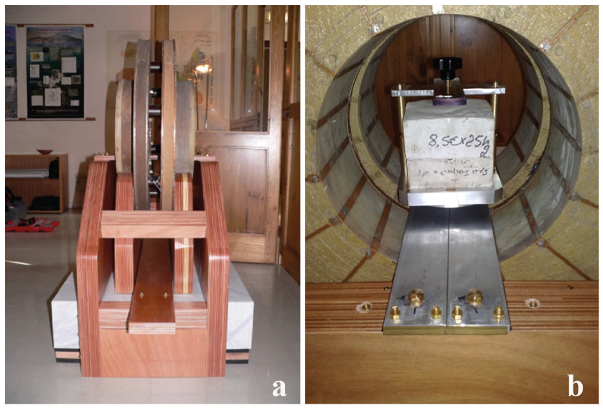
Among these instruments, rotating induction magnetometers (or inductometers) operate in accordance with Faraday’s law of electromagnetic induction. In this configuration, the rotation of the sample within the magnetic field produces a time-varying magnetic flux, which induces an electromotive force in a detection coil. This induced signal is then used to estimate weak remanent magnetic moments in the samples investigated. The first induction magnetometer designed for studying the EMF was the “reversed magnetometer” by Émile Thellier in 1938, followed by the “Bellevue magnetometer,” which was later built at the Centre National de la Recherche Scientifique (CNRS) laboratories in Bellevue (France) in 1956 [5]. In 1975, Maxime Le Goff developed at the Institut de Physique du Globe de Paris (IPGP) laboratory of Saint-Maur-des-Fossés (France) a large cell induction magnetometer based on a Helmholtz coil for measuring weak remanent magnetization [6]. One copy of this prototype instrument is currently installed at the ArchaeoLab laboratory of Consiglio Nazionale delle Ricerche, Institute of Geosciences and Earth Resources (CNR-IGG) in Pisa (Italy) (Figure 1a). Large cell induction magnetometers enable highly precise measurements, even for weakly magnetized samples, although they require large sample sizes and are characterized by the lack of automation features. These instruments are still considered prototypes and suffer from the lack of automation typical of instruments developed during that period, as well as the difficulties of shielding from the Earth’s magnetic field, especially in preparing and conditioning large samples (Figure 1b) before they are measured with this type of equipment. For this reason, all large-cell magnetometers of this type built to date have been positioned in environments with minimal possible disturbance to the local electromagnetic field (i.e., away from electrical power lines or railways, roads with heavy vehicular traffic, bodies of water, etc.). Environments with these characteristics typically occur in natural parks, such as the Migliarino San Rossore and Massaciuccoli Regional Natural Park, near Pisa, where the CNR-IGG large-cell inductometer is now located, allowing precise archaeomagnetic measurements under optimal and controlled conditions. Moreover, to shield the on-site magnetic field, this type of inductometer has been equipped with an additional compensation coil, positioned externally to the Helmholtz coil system and properly oriented and calibrated to compensate for the Earth’s magnetic field, thereby minimizing its influence during measurements. In addition, to mitigate mechanical instability, the instrument structure has been carefully designed to minimize the transmission of mechanical vibrations from the rotation axis to the detection coils. The coils are mounted on a high-mass support equipped with an anti-vibration base and are physically separated from the rotation axis, the support of which rests on an independent structure. Moreover, typical rotation speeds are kept within a range that minimizes dynamic imbalance effects while still preserving sufficient signal amplitude for reliable detection. In addition, the measurement protocol itself contributes to reducing noise-related errors. The standard measurement procedure involves rotating each sample successively in three mutually orthogonal orientations, so that each spatial component of the remanent magnetization vector can be independently measured. In practice, the sample is positioned such that two of its reference axes (X, Y, and Z) are alternately perpendicular to the rotation axis during each measurement cycle. Since the induced signal depends on the projection of the magnetic moment relative to the rotation axis and detection coils, this procedure allows the separate determination of the magnetization components along the three spatial directions. Repeating the measurements in different orientations and with opposite directions further improves accuracy by averaging random noise, compensating for minor alignment errors, and reducing the effects of sample inhomogeneity or residual magnetization associated with the sample holder. The complete three-dimensional remanent magnetization vector is subsequently reconstructed from the combination of these independent measurements.

Archaeomagnetic materials contain magnetic minerals carrying natural remanence that are mineralogically and structurally heterogeneous, leading to non-uniform magnetization caused by structural or fabric anisotropy at the grain scale (domain), or, in the case of kilns and artifacts, by magnetic refraction effect related to the geometry of the sampled structure. In addition, several secondary magnetizations can affect the rocks/material before, during, and after sampling. Among these are the Chemical Remanent Magnetization, the Viscous Remanent Magnetization (VRM), the Thermo-viscous Remanent Magnetization, the Partial Thermoremanent Magnetization, the Post-Depositional Remanent Magnetization, and the Shock Remanent Magnetization (see [7] and references therein for further details).

The identification of the magnetic minerals present in a rock, and of those carrying the remanent magnetization, is often essential for understanding its magnetic history and the processes affecting its formation and subsequent evolution. This is commonly achieved through routine thermal analysis. When heated to their Curie temperatures and beyond, remanence-carrying minerals lose their magnetic hysteresis behavior and their ability to retain permanent magnetization, becoming paramagnetic. Stepwise thermal analysis therefore not only allows the identification of the magnetic carrier or carriers, but also the detection of anomalous behavior associated with secondary magnetizations or mineralogical alterations.

The presence of anisotropy and secondary magnetization effects makes both the selection of sampling sites and the choice of sampling methods particularly critical and requires the application of specific analytical procedures for their identification and correction. These procedures are essential to isolate the primary remanent magnetization and to retrieve the original Earth’s magnetic field recorded by the material at the time of cooling below its Curie temperature. Once this primary field direction or intensity has been determined, it can be compared with appropriate secular variation curves of the geomagnetic field to estimate the age of the sampled structure.

Today, well-defined secular variation curves are available for each of the major regions characterized by magnetic homogeneity into which the globe has been subdivided, and for different chronological intervals. These curves are the result of decades of collaborative research and provide a robust framework for dating archeological structures, volcanic deposits, and other geologically relevant formations. For Europe and more generally for the circum-Mediterranean area, highly refined reference curves exist for the past 2000 years, with reliable reconstructions extending up to approximately 14,000 years BP [8].

The most critical factors of induction magnetometers are the signal strength and signal-to-noise ratio generated by the sample, which are related to the volume fraction of the sample immersed in the coil, as well as the coil structure and amplifier [9]. Earlier theoretical and experimental work by Thellier [10] on “big-sample spinner magnetometers” demonstrated that these instruments are capable of measuring the total magnetic moment of a magnetized object as the vector sum of its elementary contributions, independently of sample heterogeneity and shape. Such studies explicitly considered key parameters such as rotation frequency and sample volume and demonstrated reliable measurements for specimens with volumes on the order of 1 dm³, provided that the coil geometry and the detection circuit ensure a sufficiently homogeneous magnetic field within the measurement volume.

In this framework, this study focuses on numerical simulations, aiming to compare the magnetic field patterns generated by two different induction magnetometer configurations. The goal is to optimize coil geometry and dimensions to design a compact, high-sensitivity magnetometer, while preserving the stability and precision of traditional large-cell systems. Such improvements are expected to reduce the size of the instrument, simplify routine archaeomagnetic measurements, and thereby facilitate the transition from prototype devices to commercially produced instruments available on the geoscience market, supporting broader applications in both academic research and industrial geophysics.

2. Materials and Methods

2.1. Helmholtz Coils

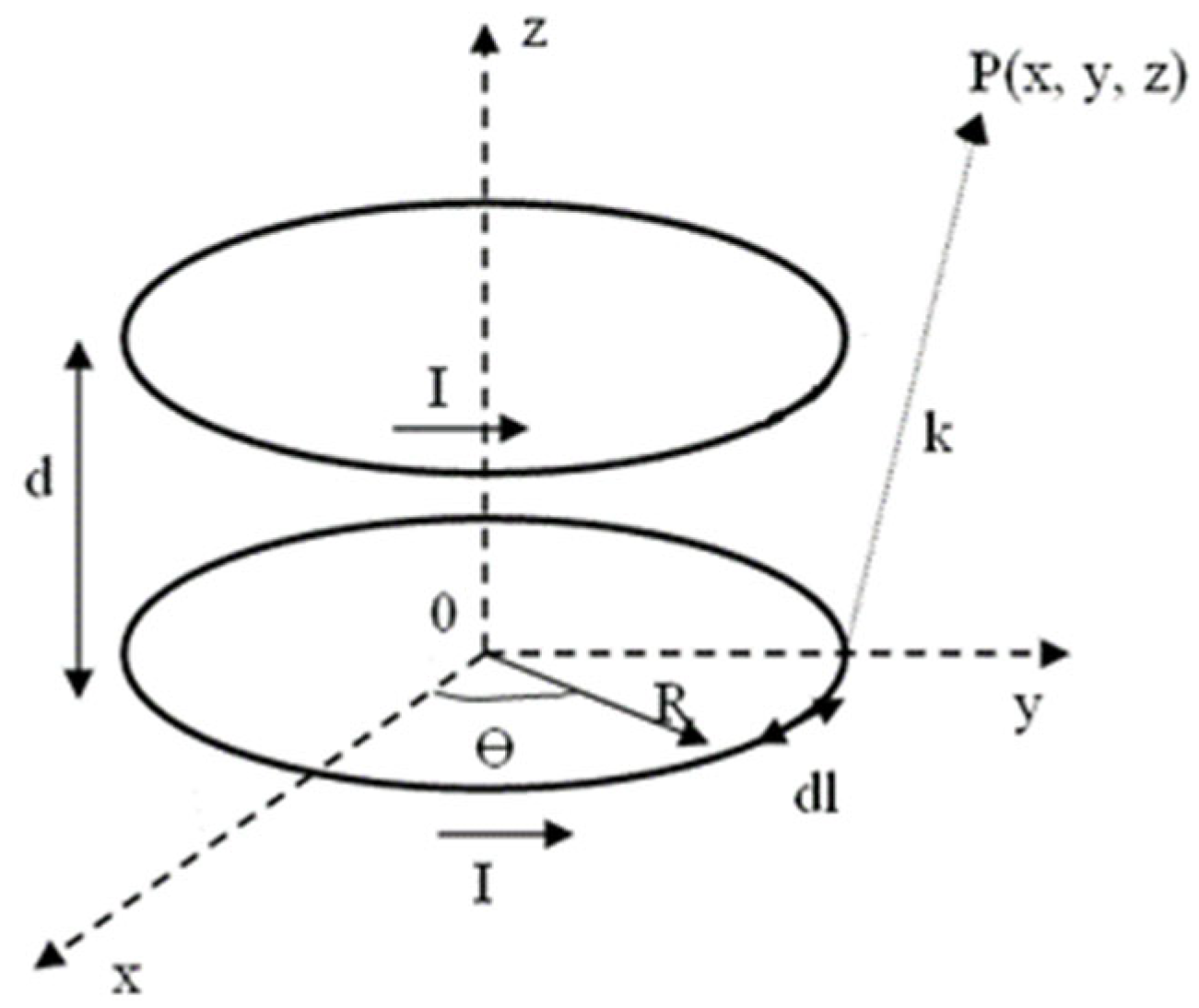
Helmholtz configuration is the simplest coil arrangement to manufacture and is able to produce a homogeneous magnetic field, with the additional advantage of easy sample positioning, both along its axial direction and orthogonally to it [11]. Such coils consist of two coaxial circular loops, made by a flat strip (rectangular shape) or circular wire (cylindrical rod) conductor, whose radius R is equal to the distance d between the two loops, and within phase currents flowing through each loop, as schematized in Figure 2.

Thanks to its configuration symmetry, such a structure produces a highly homogeneous magnetic field along the coil axis since the magnetic field’s second derivative with respect to the z-coordinate is zero at the isocentre.

2.2. Magnetic Field Calculation

Although the induction magnetometers do not generate a magnetic field but rather detect induced voltage signals produced by the magnetic moment of the sample during rotation [4], their receiving characteristics were evaluated by simulating them in transmit mode according to the reciprocity principle [12]. In particular, the static magnetic field generated by a line current I flowing in an arbitrary closed contour C can be evaluated with the magnetostatic theory, based on the Biot-Savart law [13]:

$$B\left(r\right)={\displaystyle \frac{{\mu }_{0}I}{4\pi }}{\int }_C{\displaystyle \frac{dl\times k}{k^3}}$$

(1)

where μ₀ = 4π × 10⁻⁷ Henry per meter (H/m) is the permeability of free space, dl is the infinitesimal vector tangential to contour C, and k is the distance between the observation point P and the loop conductor, as shown in Figure 2.

In the present application, this law was used to estimate the three-dimensional magnetic field distribution of two inductors based on the Helmholtz configuration by explicitly accounting for the finite cross-section of the coils, by modeling the coils as having a square cross-section and a finite number of turns. Within each coil, the turns are assumed to be evenly distributed in both the radial and axial directions, forming a regular 2D grid across the square cross-section. In the numerical implementation, the field contribution of each infinitesimal segment of current is calculated and then summed over the radial layers and over the axial layers of each coil, by implementing a double sum over the inner-to-outer radius and bottom-to-top of the coil, accounting for the finite size and thickness of the winding.

For the lower circular loop in the coil structure shown in Figure 2, the infinitesimal segment components in the conductor path for each turn are [14]:

$$dl=\left(dx,dy,dz\right)=R\left(-sin\theta ,cos\theta ,0\right)d\theta$$

(2)

and the coordinates of k vector are:

$$k=(x-Rcos\theta ,y-Rsin\theta ,z)$$

(3)

Using Equation (1), the three components of the single loop magnetic field can be calculated as:

$$B_x\left(x,y,z\right)={\displaystyle \frac{{\mu }_{0}I}{4\pi }}{\int }_0^{2\pi }{\displaystyle \frac{Rzcos\theta d\theta }{{\left[{\left(x-Rcos\theta \right)}^2+{\left(y-Rsin\theta \right)}^2+z^2\right]}^{\frac{3}{2}}}}$$

(4)

$$B_y\left(x,y,z\right)={\displaystyle \frac{{\mu }_{0}I}{4\pi }}{\int }_0^{2\pi }{\displaystyle \frac{Rzsin\theta d\theta }{{\left[{\left(x-Rcos\theta \right)}^2+{\left(y-Rsin\theta \right)}^2+z^2\right]}^{\frac{3}{2}}}}$$

(5)

$$B_z\left(x,y,z\right)={\displaystyle \frac{{\mu }_{0}I}{4\pi }}{\int }_0^{2\pi }{\displaystyle \frac{\left(R^2-Rysin\theta -Rxcos\theta \right)d\theta }{{\left[{\left(x-Rcos\theta \right)}^2+{\left(y-Rsin\theta \right)}^2+z^2\right]}^{\frac{3}{2}}}}$$

(6)

The same formalism can be used to calculate the magnetic field generated by the upper loop of the structure in Figure 3, by replacing z with z-d, then the Helmholtz coil magnetic field is given by the sum of the homologous field components.

The total magnetic field is obtained by summing the contributions from all the elementary loops that discretize the coil cross-section. Formally,

$$B\left(r\right)={\displaystyle {\sum }_{i=1}^{Nr}}{\displaystyle {\sum }_{j=1}^{Nz}}∆B_{ij}\left(r\right)$$

(7)

where each term ΔB_ij represents the magnetic field computed using the Biot–Savart law for a circular loop of radius r_i located at the axial position z_j. Here, N_r and N_z denote the number of discretization steps along the radial direction (from the inner to the outer coil diameter) and along the axial direction (from the bottom to the top of the winding), respectively.

Such equations were implemented using the IDL 6.0 (Interactive Data Language, Visual Information Solutions, Boulder, CO, USA) software tool. To increase the magnetic field homogeneity compared with that provided by the standard Helmholtz pair, the literature describes the development of structures composed of different coaxial coils [15].

2.3. Big Samples Plaster Method (BSPM)

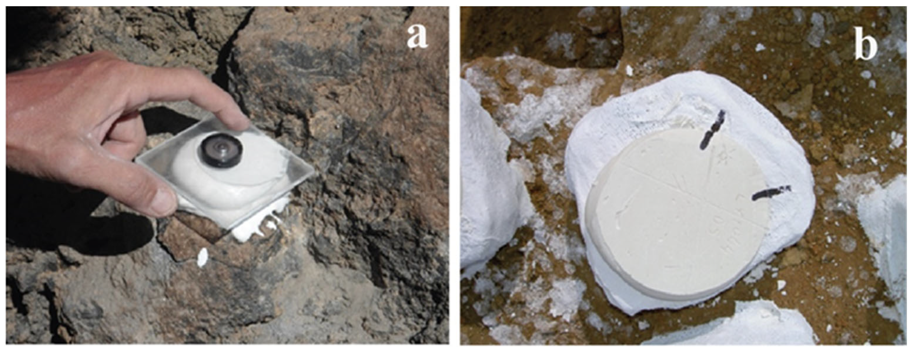
To minimize the effects of anisotropy and secondary magnetizations and to improve the analytical result of samples characterized by weak TRM components, both large-cell magnetometers and large sampling methods have been developed (e.g., [1] and references therein). The so-called “Big Samples Plaster Method” (BSPM) is a field sampling and analytical procedure in which a perfectly horizontal plaster cap, typically 5–6 cm in diameter (Figure 3), is prepared directly on rock blocks, which are then carefully extracted by hammering. For baked clay materials, plaster bandage and spatula are used instead, ensuring the preservation of fragile surfaces and maintaining the original geometry of the structure. The direction of Magnetic North and the solar azimuth line are marked on the cap, and the precise time of tracing the sun-shadow line is recorded, allowing the original orientation of the sample to be reconstructed in the laboratory with extreme precision, typically within a few tenths of a degree. In the laboratory, the oriented blocks are mounted in 12 × 12 × 12 cm plaster molds. This heavy plaster support establishes a set of three orthogonal reference axes (x, y, z), providing a robust geometric framework. The angles between the orientation data recorded in the field on the plaster cap and these reference axes are then carefully measured and entered into the analytical procedure, ensuring that the original spatial geometry of the sample is preserved throughout the analysis.

The analytical protocol, developed by the French school of Émile Thellier and described in detail in [10], is designed to minimize the VRM effect, which can be acquired when samples remain for extended periods in a magnetic field different from that in which they cooled through the Curie temperature.

This protocol involves several critical steps: (i) storing (“trainage” phase) the plaster cubes in a magnetically undisturbed environment, approximately oriented as in the field, for at least twenty days to allow any transient magnetization to equilibrate; (ii) measuring the samples in a large-cell magnetometer in the three spatial directions to record the primary TRM (direct phase); (iii) repositioning the samples in the storage environment rotated by 180° for a similar period; and (iv) repeating the measurement cycle in order to further cancel any directional VRM through vector subtraction (reverse phase). Each of these steps is carefully designed to isolate the original remanent magnetization from secondary effects, ensuring that the final results accurately reflect the geomagnetic field at the time of cooling. This meticulous procedure, while labor-intensive and time-consuming, is fundamental for producing reliable archaeomagnetic data.

3. Results

In the next two subsections, we summarize the results of analytical simulation, in terms of magnetic field patterns, of two induction magnetometers whose geometries are schematically illustrated and simulated according to the previously described theory, based on the magnetostatic numerical integration of the Biot–Savart law.

3.1. Thellier Inductor

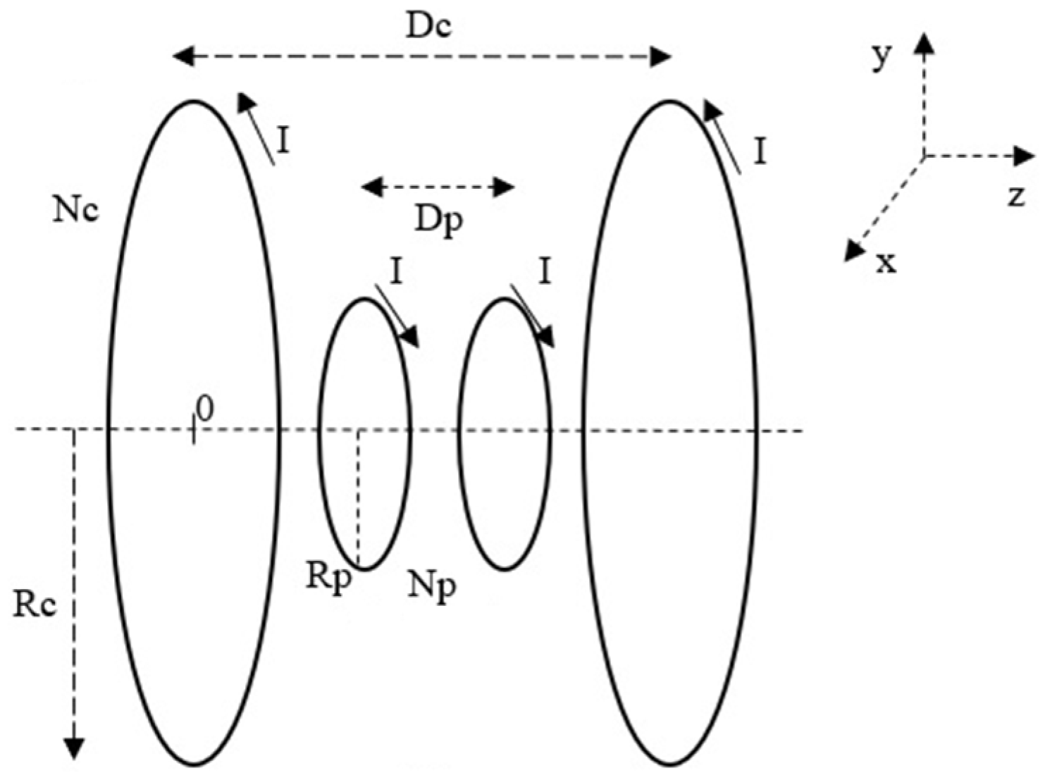
Thellier type inductor [16] consists of a couple of coaxial Helmholtz coils: the primary coil consist of 6540 loops (Np) and its Rp radius (equal to the distance Dp between the loops) is 20 cm, while the second coil, used for magnetic field compensation and whose current flows in the opposite direction to that of the primary coil, consist of 1635 loops (Nc) and its Rc radius (equal to Dc distance between loops) is 40 cm. The copper wire used in the windings has a diameter of 0.7 mm. This configuration results in a square cross-section with a side length of 80 mm for the main coils and 40 mm for the compensating coils. Figure 4 shows a schematization of this coil configuration.

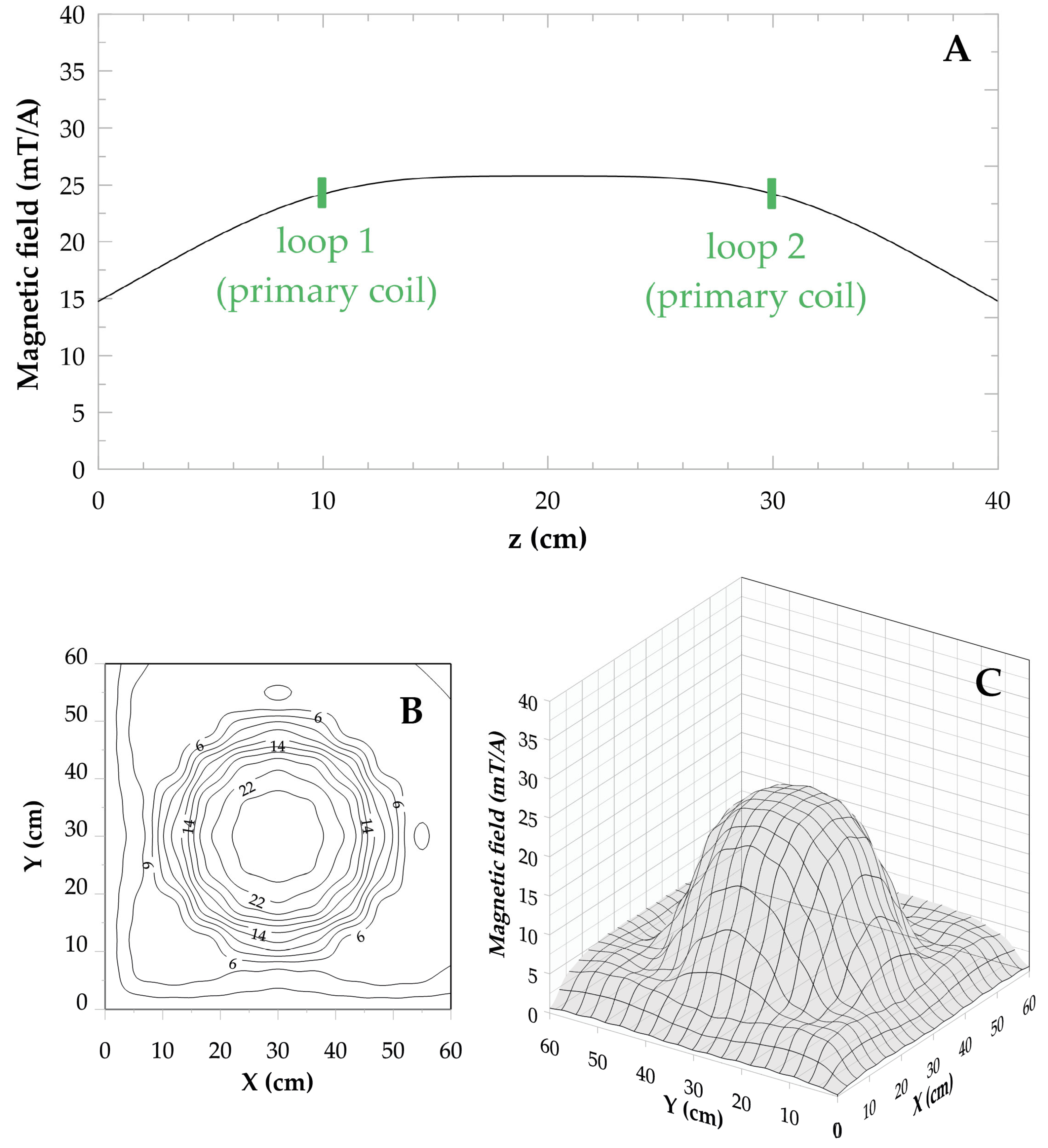
Figure 5A shows the profile plot of the normalized magnetic field pattern along the z-axis of the Thellier inductor, where the two vertical segments indicate the position of the primary coil loops. Figure 5B and Figure 5C illustrate the magnetic field contour plot and 3D plot, respectively, calculated in the transverse xy-plane at a z-coordinate of 20 cm.

The magnetic field pattern generated by the Thellier coil is very homogeneous, ensuring uniform magnetic field exposure across the sample in a region where the maximum value of the magnetic field B results in 25.8 mT/A. The magnetic field B homogeneity, defined as 100 × (max(B) − min(B))/max(B), was calculated in a field of view of 12 cm and 10 cm along the z-axis with respect to the inductor structure center. This field of view corresponds to samples of 12 × 12 × 12 cm and 10 × 10 × 10 cm, respectively. As shown in

Table 1. Simulation results for the Thellier and Le Goff coil configurations.

Inductor	Principal Coil Size (RP = DP), in cm	Field Homogeneity (%) in a z-Axis 12 cm FOV	Field Homogeneity (%) in a z-Axis 10 cm FOV	Field Homogeneity (%) in a Cubic 12 cm3 FOV	Field Homogeneity (%) in a Cubic 10 cm3 FOV	Magnetic Field Intensity (mT/A)	K (%) in the 12 cm3 Cubic Faces	K (%) in the 10 cm3 Cubic Faces
Thellier	20	98.89	99.53	94.49	97.45	25.8	0.94	0.47
	15	96.80	98.57	83.93	92.33	35.6	3.27	1.65
	25	99.52	99.80	97.72	98.94	19.9	0.36	0.18
Le Goff	20	99.49	99.77	93.47	96.82	37.4	0.89	0.62
	15	97.23	98.46	82.91	91.71	52.4	2.99	1.42
	25	99.70	99.78	96.57	98.21	28.4	1.07	0.70
Helmholtz N = 6540	20	99.15	99.50	95.12	97.75	29.5	0.83	0.41
Helmholtz N = 1635	40	99.94	99.97	99.71	99.86	3.7	0.04	0.02

, for the smaller sample size, the magnetic field homogeneity increases. By decreasing the Thellier primary coil radius and their relative distance from 20 cm to 15 cm, the magnetic field intensity increases, but the field homogeneity decreases, whereas increasing the radius and distance up to 25 cm, the magnetic field intensity decreases and the field homogeneity increases.

3.2. Le Goff Inductor

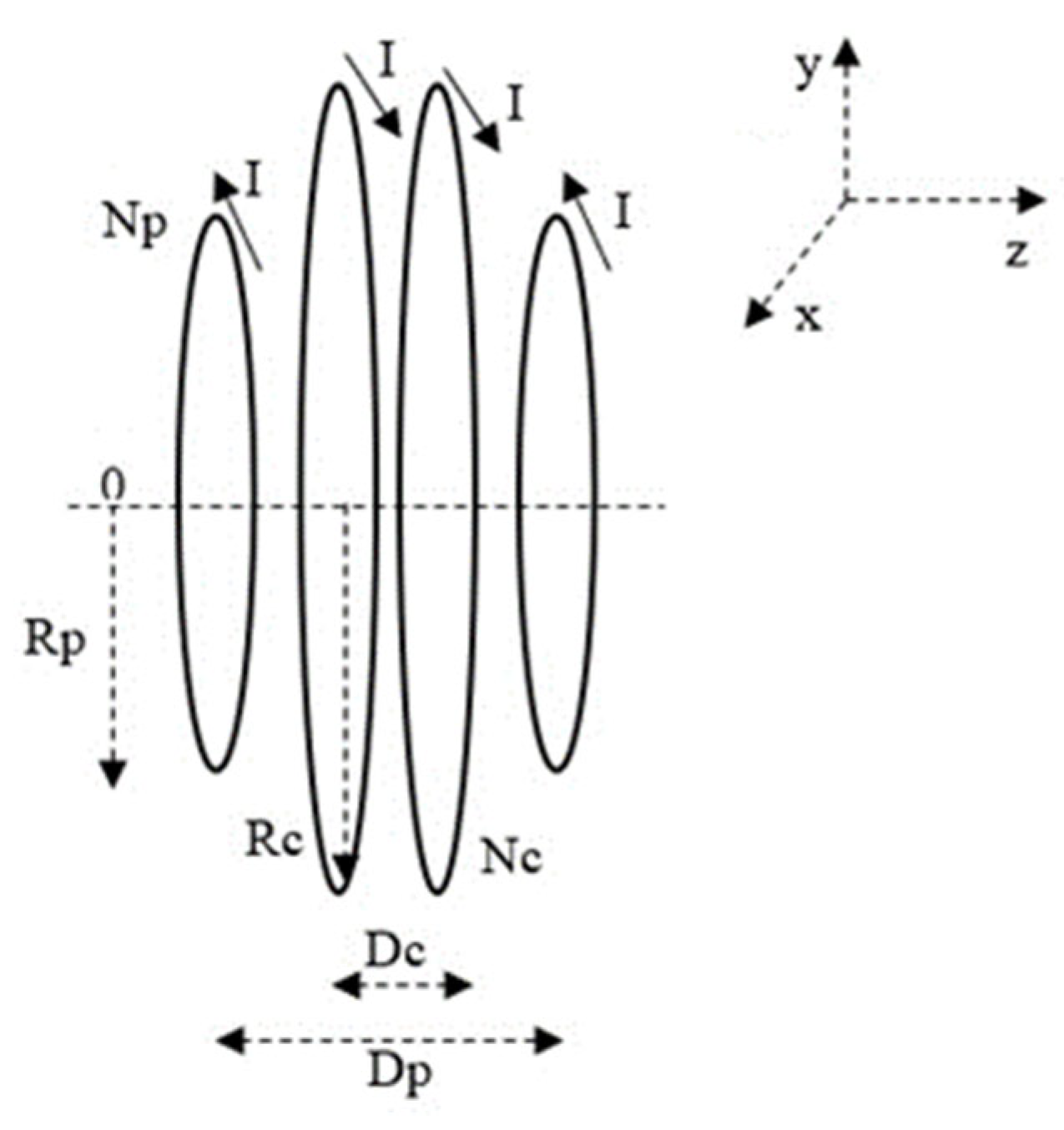
The Le Goff inductor [17] consists of a Helmholtz coil acting as the primary coil (with Rp radius equal to the inter-coil distance Dp = 20 cm and Np = 10,000 turns) and a secondary coil for magnetic field compensation (Rc radius = 40 cm, Dc distance between loops = 10 cm, Nc number of loops = 2500) carrying an opposite electric current I. The coil configuration adopts the same winding structure as the Thellier inductor. Figure 6 depicts a schematic representation of the Le Goff inductor.

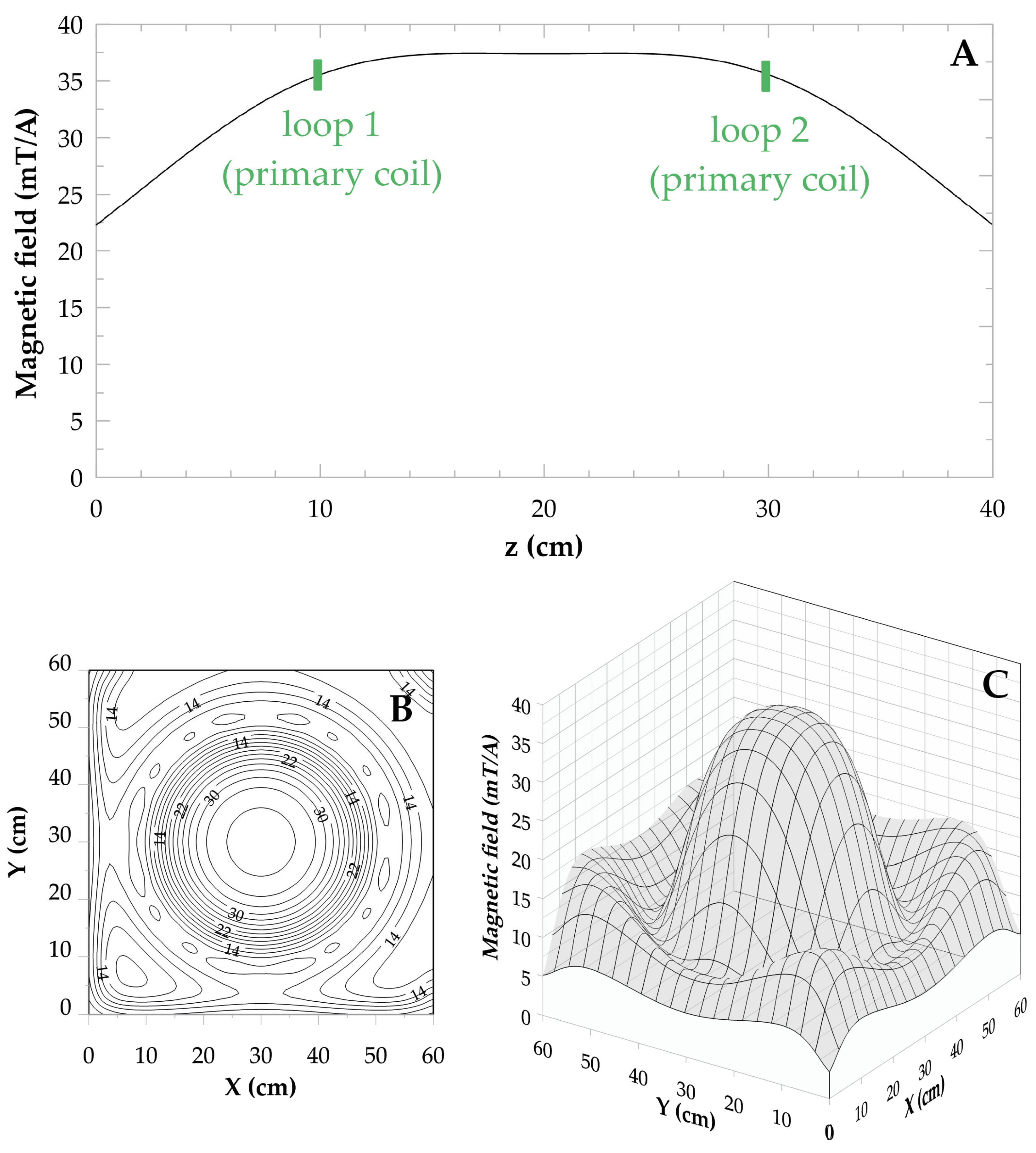
Figure 7A shows the profile plot of the normalized magnetic field pattern along the z-axis in the space between the two loops of the principal coil, located as indicated by the two vertical segments. Figure 7B and Figure 7C illustrate the magnetic field contour plot and 3D plot, respectively, calculated in the transverse xy-plane at a z-coordinate of 20 cm (at the structure center).

The maximum value of the magnetic field is 37.4 mT/A. Table 1 reports the magnetic field (B) homogeneity evaluated within a field of view (FOV) of both 12 cm and 10 cm along the z-axis relative to the center of the inductor structure. As observed for the Thellier inductor, the magnetic field homogeneity increases when considering the smaller sample size. By decreasing the Le Goff principal coil radius and the distance between the coils from 20 cm to 15 cm, the magnetic field intensity increases, and the field homogeneity decreases, whereas increasing the radius and distance up to 25 cm, the magnetic field intensity decreases and the field homogeneity increases. Overall, compared to the Thellier coil, the Le Goff type configuration achieves higher magnetic field intensity and a similar field homogeneity. To perform a comparison with the standard configuration, two Helmholtz inductors (a 20 cm radius/N = 6540 turns and a 40 cm radius/N = 1635 turns) were also simulated. However, the sample embedded in the plaster is unlikely to be perfectly centered with respect to the rotation axis. Under such conditions, magnetization components in the x and y directions that are offset from the axis may be partially projected onto the z direction during rotation. This geometrical misalignment may therefore produce an apparent z-component magnetization signal. To evaluate the off-axis behavior of the magnetic field generated by the coil systems, we considered: (1) the spatial variation in the magnetic field magnitude within cubes with side lengths of 10 cm and 12 cm centered on the midpoint between the coils; (2) the ratio K between the transverse (Bx and By) and axial (Bz) magnetic field components at the boundaries of the sample region (i.e., evaluated on the six faces of the cube). This parameter provides an estimate of the maximum contribution of off-axis fields, accounting for potential sample misalignment and ensuring that any apparent axial magnetization arising from off-axis components during rotation is properly taken into consideration. In particular, the K parameter was calculated as the ratio between the maximum absolute values of the Bx and By field components and the maximum absolute value of the axial Bz component evaluated on the six faces of the central cube, according to:

K = max(∣Bx∣faces, ∣By∣faces)/max(∣Bz∣faces).

3.3. Experimental Benchmark Validation

To assess the reliability of the developed simulation software, the magnetic field generated by a Helmholtz coil configuration previously characterized experimentally in the literature [18] was numerically simulated. The investigated Helmholtz pair (coil radius a = 65 cm, inter-coil distance d = 65 cm, and N = 250 turns per coil, wound around the edge of a 0.635 cm thick plywood board) was experimentally characterized by supplying the coils at 60 Hz and measuring the magnetic field using a flux probe.

Table 2. Simulated and experimentally measured magnetic field values for a Helmoltz coil [18].

Direction	Coordinate	Normalized Simulated Field (Bsim)	Normalized Measured Field (Bexp)	Relative Error (%)
Axial	z/a = 0.0	1.000	1.000	0.00
	z/a = 0.1	1.000	1.001	0.10
	z/a = 0.2	0.998	1.000	0.20
	z/a = 0.3	0.991	0.994	0.30
	z/a = 0.4	0.975	0.974	0.10
Radial	r/a = 0.0	1.000	1.000	0.00
	r/a = 0.1	1.000	1.002	0.20
	r/a = 0.2	0.999	1.001	0.20
	r/a = 0.3	0.996	0.998	0.20
	r/a = 0.4	0.987	0.990	0.30
	r/a = 0.5	0.967	0.968	0.10
	r/a = 0.6	0.925	0.928	0.32
	r/a = 0.7	0.851	0.849	0.23

compares the simulated and experimentally measured magnetic field values. The values were normalized with respect to the magnetic field value at the center of the coil system (z/a = 0 for axial measurements and r/a = 0 for radial measurements, where z/a and r/a represent the axial and the radial coordinates normalized to the coil radius, respectively). The percentage error was evaluated as 100 × |Bsim − Bexp|/Bexp.

Excellent agreement was observed both along the coil axis and in the radial direction within the central plane, confirming the reliability of the adopted numerical methodology in reproducing experimentally measured magnetic-field distributions. The discrepancy between simulated and experimental values remained below 0.5% at all the measurement positions considered.

4. Discussion

4.1. Limitations and Assumptions of the Simulation Approach

The numerical simulations presented in this study are based on an idealized representation of the induction magnetometer coils and rely on several simplifying assumptions that should be explicitly considered when interpreting the results. In particular, the magnetic field calculations are performed using the Biot–Savart law assuming infinitely thin conductors, perfectly circular coils, and uniform current distribution, while neglecting the finite cross-section of the wires and possible manufacturing imperfections. Moreover, external magnetic disturbances and small coil misalignments that may occur in actual experimental conditions are not considered. Despite these simplifications, the adopted approach provides a robust first-order description of the magnetic field geometry and homogeneity within the measurement volume. As a result, the simulations are well-suited for comparative analysis between different coil configurations and for guiding design choices, though experimental validation remains essential for fully characterizing instrument performance under operational conditions.

4.2. Archeomagnetic Implications

The Big Samples Plaster Method (BSPM), first introduced by Émile Thellier and later refined through subsequent improvements, was specifically developed for oriented samples intended for analysis using the Large Cell Induction Magnetometer developed by Maxime Le Goff in 1975. This approach enables high-precision archaeomagnetic measurements, exceeding the accuracy typically obtained using diamond coring techniques, which often require follow-up analyses with spinner or cryogenic magnetometers. The remarkable precision of BSPM is derived from a combination of a sampling procedure that preserves large, intact specimens and a sufficiently large measurement cell capable of fully accommodating them, thereby minimizing disturbances to the natural remanent magnetization [1,10].

The simulations performed in this study indicate that the maximum effective sample size for accurate measurements is approximately 12 cm. However, for optimal results and to preserve the highest possible magnetic field homogeneity within the measurement volume, samples should preferably not exceed 10 cm in size. Exceeding the 12 cm threshold does not provide any significant improvement in measurement quality, even for specimens characterized by very weak remanent magnetization, because the increase in sample size does not compensate for the potential decrease in field uniformity. This finding has important practical implications for instrument design and sample preparation. It suggests induction magnetometers with smaller measurement cells could be developed, while still preserving the analytical advantages of the BSPM approach. At the same time, field samples could continue to be conditioned and oriented following the same meticulous procedures currently employed, while being housed in slightly smaller plaster molds of approximately 10 cm rather than the traditional 12 cm. Such an adaptation would preserve the same level of precision and sensitivity in their archaeomagnetic analyses, while potentially reducing the size, weight, and material requirements of both the measurement equipment and sample supports, thereby improving the efficiency and practicality of routine measurements.

Alternative methods recently proposed in the literature for analyzing large samples using spinner magnetometers [19] are certainly of interest, but differ from our approach, which is based on directional analyses of declination and inclination, since they focus exclusively on intensity measurements. Furthermore, the use of commercial fluxgate sensors (e.g., Mag-03MS100, Bartington Instruments Ltd., Witney, UK) is not suitable in this context due to sensitivity limitations, which are significantly exceeded by the performance of our instrument [9].

Finally, to assess the off-axis contributions of the magnetic field, we computed the ratio of the transverse components (Bx and By) to the principal axial component (Bz) on the faces of the central cube. This ratio provides a quantitative measure of field purity along the axial direction: smaller ratios indicate that the field is predominantly aligned along z, whereas larger ratios reflect more significant transverse components. Such transverse components are particularly relevant when the sample is not perfectly centered, as they can manifest as apparent z-axis magnetization upon rotation. Our results, which show that reducing the cube size led to a decrease in this ratio, indicate that the field within the smaller cube is more purely axial and thus less prone to off-axis artifacts.

Moreover, the results show that the 20 cm classical Helmholtz configuration provides a level of field homogeneity within the cubic sample volume that is comparable to that of the standard Thellier and Le Goff geometries. Additionally, the ratio between transverse and longitudinal field components is found to be slightly lower for the Helmholtz configuration, indicating a marginally reduced sensitivity to off-axis effects. The magnetic field intensity at the center is also slightly lower for the Helmholtz configuration. However, these differences remain small over the spatial extent of the sample. Therefore, when evaluated under realistic experimental conditions relevant to archeomagnetic applications, all configurations provide comparable performance in terms of field uniformity and control of transverse components. The choice of coil geometry may therefore depend primarily on practical considerations, such as ease of construction and accessibility to the sample, rather than on field uniformity alone.

5. Conclusions

This study provides a detailed comparison between two different induction magnetometer configurations, both based on Helmholtz coil design, with particular focus on their magnetic field patterns as calculated using the Biot-Savart law. The simulation method described here is straightforward to implement mathematically, allowing it to be incorporated into a standard computational software package and providing accurate results within a relatively short computational time. This approach offers a flexible and efficient way to evaluate the performance of different coil arrangements, enabling researchers to assess the uniformity and intensity of the magnetic field generated by each configuration.

Moreover, the simulation framework allows for the modeling of inductors with varying sizes and geometries, which can be tailored to accommodate smaller sample volumes. By adjusting the input parameters in the simulation, it is possible to predict the resulting magnetic field homogeneity and intensity, thereby optimizing the design for specific measurement requirements. This capability is particularly valuable for improving analyses of weakly magnetized specimens, where higher magnetic field uniformity directly translates into more precise and reliable results.

The insights gained from these simulations can be directly applied to the development of a new generation of optimized induction magnetometers. Such instruments would feature coils and measurement cells of reduced dimensions while preserving the high sensitivity, stability, and accuracy characteristics of traditional large-cell systems. This miniaturization could offer several practical advantages, including reduced instrument footprint, lower material and construction costs, and easier handling of samples, without compromising analytical performance.

Future work could involve the experimental validation of the optimized induction magnetometer configurations proposed in this study. Prototype instruments may be constructed according to the simulated coil geometries and cell dimensions, enabling preliminary tests on well-characterized reference samples. Such experiments would aim to assess the precision, sensitivity, and reproducibility of the devices, particularly when measuring weakly magnetized archaeomagnetic specimens. Careful calibration and repeated measurements could help identify potential limitations or sources of systematic error, providing valuable feedback for further refinement of the design.

Prospective developments may also explore additional miniaturization of the instrument without compromising the stability and high sensitivity observed in traditional large-cell systems. The implementation of semi-automated sample positioning and data acquisition protocols could enhance measurement efficiency and reduce operator-induced variability. Furthermore, adjustable coil arrangements might allow for the analysis of samples with varying dimensions while maintaining optimal magnetic field homogeneity. Although these developments remain speculative at this stage, they offer a plausible roadmap for translating the current simulation results into practical, high-performance archaeomagnetic instrumentation. If successful, such innovations could significantly facilitate routine laboratory analyses, improve measurement accuracy, and expand the applicability of archaeomagnetic techniques in both research and applied geoscience contexts.

References

1. Le Goff, M.; Gallet, Y.; Warme, N.; Genevey, A. An updated archeomagnetic directional variation curve for France over the past two millennia, following 25 years of additional data acquisition. Phys. Earth Plan. Int. 2020, 309, 106592. [Google Scholar] [CrossRef] [Scilit]
2. Courtillot, V.; Le Mouël, J.-L. The study of Earth’s magnetism (1269–1950): A foundation by Peregrinus and subsequent development of geomagnetism and Paleomagnetism. Rev. Geoph. 2007, 45, RG3008. [Google Scholar] [CrossRef] [Scilit]
3. Genevey, A.; Gallet, Y.; Boudon, G. Secular variation study from non-welded pyroclastic deposits from Montagne Pelee volcano, Martinique (West Indies). Earth Planet. Sci. Lett. 2002, 201, 369–382. [Google Scholar] [CrossRef] [Scilit]
4. Collinson, D.W. Methods in Rock Magnetism and Palaeomagnetism; Chapman and Hall: London, UK, 1983. [Google Scholar]
5. Thellier, E. Le champ magnétique terrestre fossile. Nucleus 1966, 7, 1–35. [Google Scholar]
6. Le Goff, M.; Daly, L.; Dunlop, D.J.; Papusoi, C. Émile Thellier (1904–1987), a pioneer in studies of the “fossil” Earth’s magnetic field. In Historical Events and People in Aeronomy, Geomagnetism and Solar-Terrestrial Physics; Schröder, W., Ed.; Arbeitskreis Geschichte Geophys. und Kosm. Phys.: Potsdam, Germany, 2006; pp. 98–112. [Google Scholar]
7. Butler, R.F. Paleomagnetism: Magnetic Domains to Geological Terranes; Blackwell Scientific Publications: Oxford, UK, 1992. [Google Scholar]
8. Pavón-Carrasco, F.J.; Rodríguez-González, J.; Osete, M.L.; Torta, J.M. A matlab tool for archaeomagnetic dating. J. Archaeol. Sci. 2011, 38, 408–419. [Google Scholar] [CrossRef] [Scilit]
9. van Oorschot, B.P.J.; Ridler, P.F. A sensitive spinner magnetometer using a coil detector. Geophys. J. Int. 1976, 45, 569–581. [Google Scholar] [CrossRef] [Scilit]
10. Thellier, E. A “Big Sample” Spinner Magnetometer. Methods in Palaeomagnetism. Dev. Solid Earth Geophys. 2013, 3, 149–154. [Google Scholar]
11. Mispelter, J.; Lupu, M.; Briguet, A. Nmr Probeheads for Biophysical and Biomedical Experiments: Theoretical Principles and Practical Guidelines; Imperial College Press: London, UK, 2006. [Google Scholar]
12. Hoult, D.I. The principle of reciprocity in signal strength calculations? A mathematical guide. Concepts Magn. Reson. 2000, 12, 173–187. [Google Scholar] [CrossRef] [Scilit]
13. Jin, J. Electromagnetic Analysis and Design in Magnetic Resonance Imaging; CRC: Boca Raton, FL, USA, 1999. [Google Scholar]
14. Giovannetti, G. Comparison between circular and square loops for low-frequency Magnetic Resonance applications: Theoretical performance estimation. Concepts Magn. Reson. Part B 2016, 46B, 146–155. [Google Scholar] [CrossRef] [Scilit]
15. Ghaly, S.M.A.; Al-Snaie, K.A.; Mohammad, O.K. Spherical and Improved Helmholtz Coil with High B1 Homogeneity for Magnetic Resonance Imaging. Am. J. Appl. Sci. 2016, 13, 1413–1418. [Google Scholar] [CrossRef] [Scilit]
16. Thellier, E. Methods of Sample Collection and Orientation for Archaeomagnetism. Methods Palaeomagnetism. Dev. Solid Earth Geophys. 2013, 3, 16–20. [Google Scholar]
17. Le Goff, M. Inductomètre à Rotation Continue Pour la Mesure de Faibles Aimantations Rémanentes et Induites en Magnétisme des Roches. Master’s Thesis, CNAM, Paris, France, 1975. [Google Scholar]
18. Bell, G.B.; Marino, A.A. Exposure system for production of uniform magnetic fields. J. Bioelectr. 1989, 8, 147–158. [Google Scholar] [CrossRef] [Scilit]
19. Uehara, M.; Gattacceca, J.; Quesnel, Y.; Lepaulard, C.; Lima, E.A.; Manfredi, M.; Rochette, P. A spinner magnetometer for large Apollo lunar samples. Rev. Sci. Instrum. 2017, 88, 104502. [Google Scholar] [CrossRef] [Scilit] [PubMed]
Figure 1. Induction magnetometer at CNR-IGG of Pisa. (a) Lateral view of large-cell induction magnetometer with Le Goff configuration of the Helmholtz coils (b) Frontal view of the large-cell loaded with 12 cm cubic molds inside (photo by C.P.).
Geosciences 16 00220 g001
Figure 2. Helmholtz coil sketch used for magnetic field pattern calculation.
Geosciences 16 00220 g002
Figure 3. Sampling method: (a) preparation of a perfectly horizontal plaster cap on a lava block during field sampling; (b) marking of the sun-shadow line and the magnetic north direction on a kiln fragment wrapped with a plaster bandage, allowing accurate orientation of the sample for subsequent laboratory analyses. (Photo by C.P.).
Geosciences 16 00220 g003
Figure 4. Schematic representation of the setup of coils in the Thellier inductor.
Geosciences 16 00220 g004
Figure 5. Thellier inductor magnetic field pattern: (A) variation in the magnetic field along the z-axis, the segments indicate the principal coil position, (B) contour plot at z = 20 cm, and (C) three-dimensional plot at z = 20 cm providing a comprehensive visualization of the field’s geometry and uniformity within the measurement region.
Geosciences 16 00220 g005
Figure 6. Schematic representation of the setup of coils in Le Goff inductor.
Geosciences 16 00220 g006
Figure 7. Le Goff inductor magnetic field pattern: (A) variation in the magnetic field along the z-axis, the segments indicate the principal coil position, (B) contour plot at z = 20 cm, and (C) 3D plot at z = 20 cm providing a clear view of the field’s geometry and uniformity.
Geosciences 16 00220 g007