Article

Subsoil Characterisation in an Abandoned Dam in Central Mexico Using Geoelectrical Methods

by
Ximena Michelle Trejo-Martínez
1,
Omar Delgado-Rodríguez
1,*,
José Alfredo Ramos-Leal
1,
Héctor José Peinado-Guevara
2 and
Simón Eduardo Carranco-Lozada
3
1
Instituto Potosino de Investigación Científica y Tecnológica, Camino a la Presa San José 2055, Lomas 4ta Sección, San Luis Potosí 78216, Mexico
2
Faculty of Economic and Administrative Sciences, Autonomous University of Sinaloa, Guasave 81100, Mexico
3
Instituto Politécnico Nacional (IPN), CECyT 15 D.A.E., Cda. Gaston Melo 41, Tenantitla, Milpa Alta, San Antonio Tecómitl, Mexico City 12100, Mexico
*
Author to whom correspondence should be addressed.
Geosciences 2026, 16(6), 209; https://doi.org/10.3390/geosciences16060209
Submission received: 26 March 2026 / Revised: 8 May 2026 / Accepted: 18 May 2026 / Published: 22 May 2026
(This article belongs to the Section Geophysics)

Abstract

In central Mexico, ground failure and subsidence have accelerated, as evidenced by the Villa de Reyes graben, particularly at the El Hundido Dam, with the primary cause attributed to groundwater overexploitation. This study integrates electromagnetic profiling (EMP), electrical resistivity tomography (ERT), and transient electromagnetic (TEM) surveys to determine the origin of the fractures at the El Hundido Dam. Based on the TEM survey, a geoelectric section was obtained that models the depth and morphology of the igneous bedrock. At the El Hundido Dam, the igneous basement exhibits convex deformation due to transpressional stresses, which favours the formation of a positive flower-type fault structure. Deformations caused by the basement topography and the fault system are evident in the 100 m-thick Quaternary sequence, as revealed by ERT studies. ERT and EMP surveys showed the presence of a clayey layer that acted as a barrier to surface water infiltration, allowing it to be stored in the past, and which is now destroyed by fractures. Although the drop in the water table has contributed to polygonal cracking, hydro-compaction, and ground subsidence, local tectonics is the primary factor controlling subsoil faulting at the El Hundido Dam.

1. Introduction

Ground failure and land subsidence are phenomena that affect several regions worldwide [1,2]. They are caused by natural factors such as tectonic features, geological faults, regional seismic activity [3], hydro-compaction [4], and karst processes [5], as well as anthropogenic factors, such as overexploitation of groundwater and changes in land use [2,6]. Over the past two decades, synthetic aperture radar interferometry (InSAR) has become an effective tool worldwide for studying ground subsidence [7].
In Mexico, fracturing and land subsidence have intensified in parallel with rapid urban expansion and increased groundwater extraction [8]. Approximately 16 cities in Mexico exhibit high rates of ground failure and land subsidence [9], accelerated by changes in agricultural land use due to massive urban and industrial infrastructure construction and the consequent increase in groundwater withdrawal. In Ciudad Guzmán, in the state of Jalisco [3], and in Morelia city, in the state of Michoacán [10], InSAR studies have shown that critical damage to urban infrastructure and subsidence associated with fracture zones result from a combination of natural and anthropogenic factors. Mexico City deserves particular attention due to the high rate of subsidence and ground fracturing, as demonstrated by InSAR surveys [11,12]. In the city of San Luis Potosí, SLP, Persistent Scatter Interferometry (PSI) studies conducted by Navarro-Hernández et al. [13] demonstrated that land subsidence is mainly due to excessive groundwater extraction.
One of the most representative cases of land subsidence in Mexico occurs in the aquifer system of the Mexico Basin. This phenomenon represents a major challenge for water management in Mexico City because understanding and modelling this process requires a clear conceptual model that integrates the factors that generate it together with the stratigraphy, the geomechanical properties of the subsurface, and field data that allow the causes of ground subsidence to be identified before numerical modelling is carried out [14].
Geophysical methods are also effective tools for the study of land subsidence and associated faulting. Geophysical methods rely on measurable physical properties to identify and delineate subsurface features, providing reliable characterisation for civil engineering and geological studies through non-invasive, non-destructive techniques that enable accurate imaging of underground conditions without permanently altering the ground structure [15].
The analysis of the three-dimensional deformation velocity field combined with transient electromagnetic (TEM) surveys revealed the tectonic influence on land subsidence in Zamora, Mexico, where the maximum subsidence and its spatial pattern coincide with the main tectonic graben, indicating that understanding this phenomenon requires not only analysing subsidence rates and their spatial distribution but also considering the configuration of the bedrock and the thickness of the overlying sediments [16].
Dindi [15] evaluated the effectiveness of electromagnetic, magnetic and gravity methods at a site located southwest of the town of Nakuru in Kenya. Very-low-frequency electromagnetic and magnetic studies showed a good response in areas affected by subsidence and faulting. The gravimetric method, although it responded similarly in some cases, did not in others due to its low sensitivity in detecting density contrasts in areas with narrow fractures. In Querétaro city, Mexico, Pacheco et al. [17] applied the gravimetric method to model the topographic variations of the aquifer base, which they define as responsible for the differential subsidence and associated ground failures.
Geoelectrical methods such as TEM sounding, electrical resistivity tomography (ERT) and spontaneous potential (SP) have been successfully applied to identify groundwater-rich zones and infiltration pathways, allowing the development of three-dimensional subsurface models that reveal how aquifer recharge commonly occurs through fractures and weathered zones [18].
Monge-Cerda et al. [19] conducted a geological and geophysical study in the southern portion of the Villa de Reyes Graben, at four sites located near the municipalities of Villa de Reyes (San Luis Potosí) and Jaral de Berrios (Guanajuato) (Figure 1A), using electromagnetic profiling (EMP), ERT, and Ground Penetrating Radar (GPR) methods. The EMP results showed high apparent resistivity anomalies associated with unfilled fractures in the subsoil that do not always outcrop at the surface. The application of the ERT method enabled more accurate characterisation of the areas defined by the EMP, revealing a system of nearly vertical fractures that join at greater depth, consistent with field evidence of positive and negative flower-type structures. These structures could not be clearly identified using the GPR method, particularly at the El Hundido site, in the state of San Luis Potosí (Figure 1A,B), presumably due to the high clay content of the alluvial unit, which caused significant signal attenuation and reduced the ability to delineate the fractures.
Monge-Cerda et al. [19] conducted a 1120 m long ERT survey at the El Hundido Dam, with an electrode spacing of 10 m (medium resolution), reaching a depth of 110 m. Based on the ERT results and direct field observations, they concluded that the predominant stress regime is transtensional, resulting in negative flower-shaped faults. However, they also considered indications of transpressional deformation from GPR analysis and the positive flower-type deformations observed in the dam wall. The results of Monge-Cerda et al. [19] demonstrate that surface geological structures can be identified. However, techniques such as GPR and EMP have a significant limitation in terms of their depth range. This restriction means that current knowledge focuses primarily on surface levels, leaving a significant gap in the characterisation of structures at greater depths, particularly in the basement beneath the sedimentary sequence. Consequently, there is a clear gap in deep geophysical research, necessitating the exploration and implementation of alternative methods capable of reaching greater depths to assess the continuity and presence of such structures at deeper levels.
Higher-resolution, deeper geophysical studies are needed to determine whether the fracturing of the subsoil beneath the El Hundido Dam is due to natural causes, such as geological faults, or exclusively to human factors, such as the overexploitation of groundwater. To address this research gap, electrical and electromagnetic studies were conducted using EMP, ERT, and TEM methods.
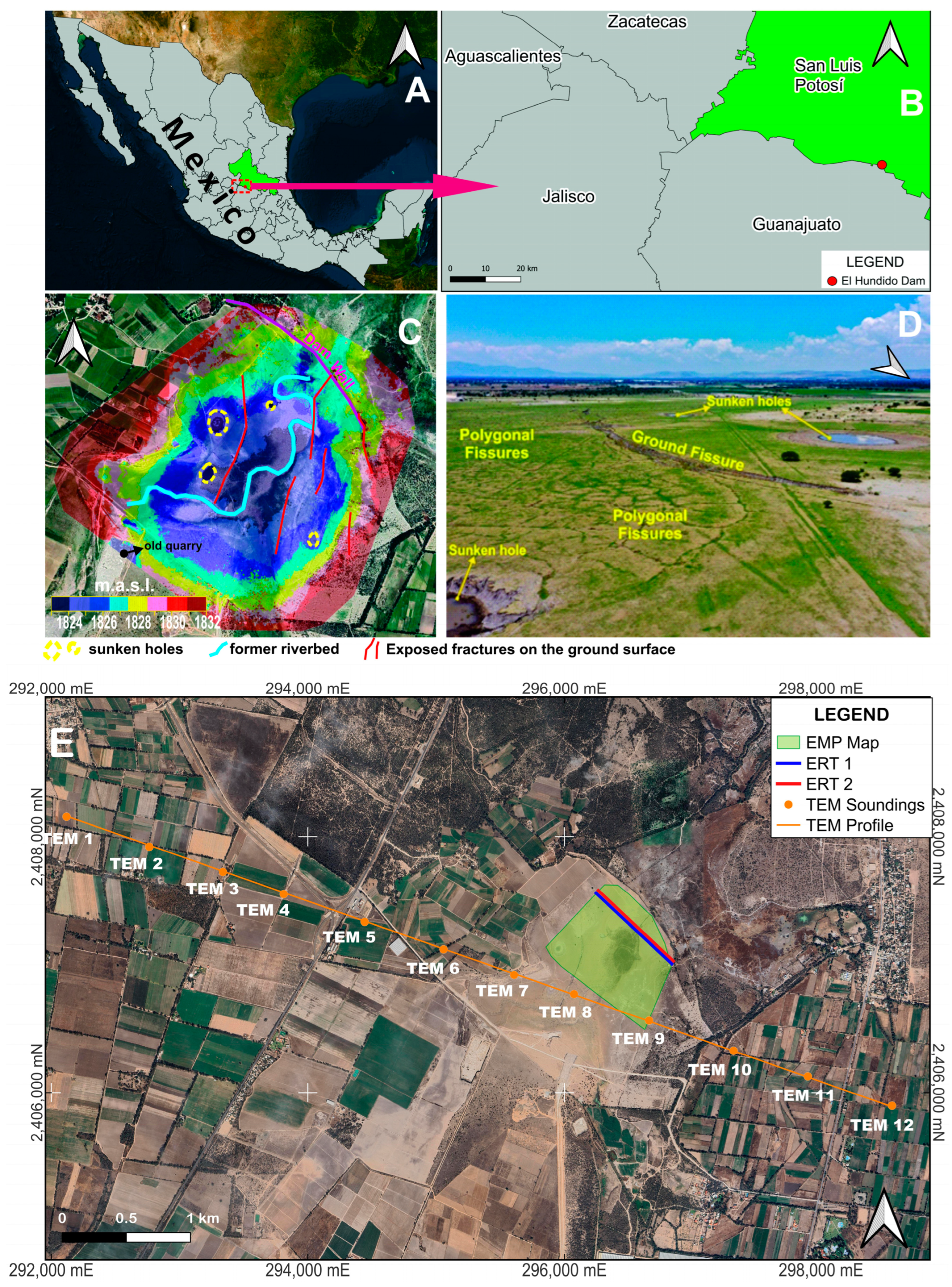
El Hundido is an old dam that failed due to structural rupture and the presence of large ground fissures and sunken holes upstream, which prevent water retention (Figure 1C,D). The process of ground failures has accelerated over the last decade, with evidence of land subsidence affecting agricultural and livestock farming in the region.

Study Site Description

The former dam is located next to the town of El Hundido (Figure 1), in the municipality of Villa de Reyes, in southern San Luis Potosí, Mexico (Figure 1B).
The El Hundido Dam site has UTM-WGS84 coordinates in zone 14Q 296,279 m E and 2,406,860 m N. It is located on the old La Hilada or El Refugio river (Figure 1C). According to CONAGUA [20], it was built by private owners in 1952 to carry water to the San Miguel Ejido. However, because it is very old, there are no official records of its construction or a reliable chronology of events that have occurred within it, such as the rupture of the dam wall and its causes, so its history, purpose, and current state raise many questions [21]. At present, the former dam basin comprises an extensive plain of around 240 hectares, characterised by solonchak soils, typical of floodplains, used for grazing cattle and sheep. In the Villa de Reyes valley, the average annual temperature in the study area is 16 to 18 °C, and the total annual precipitation recorded is 376 mm [22].
Currently, large fissures can be seen on the ground surface in the El Hundido Dam basin, reaching a maximum width of 7 m and a depth of 10 m (Figure 1D). These fractures vary in orientation from N-S to SW-NE (Figure 1C). Although previous studies suggest the existence of positive–negative flower-type fractures, the geological-structural model is still undetermined for the El Hundido Dam [19]. The riverbed that supplied the reservoir is now a paleochannel filled with highly permeable granular sediments. Across the central section of the dam, particularly in the north–central part, there is a notable presence of polygonal fractures (Figure 1C,D), which creates a “vein system” that facilitates the dissolution and infiltration of fine sediments into the subsoil, especially during the rainy season. This process can intensify in certain areas, causing ductile settlement of the overburden and creating a suffosion sinkhole [23,24]. At the study site, suffosion sinkholes of varying diameter range from a few to tens of meters (Figure 1C,D). Hereinafter, suffosion sinkholes will be referred to as “sunken holes”, to avoid associating the term “sinkhole” with dissolution processes in carbonate environments (karst).
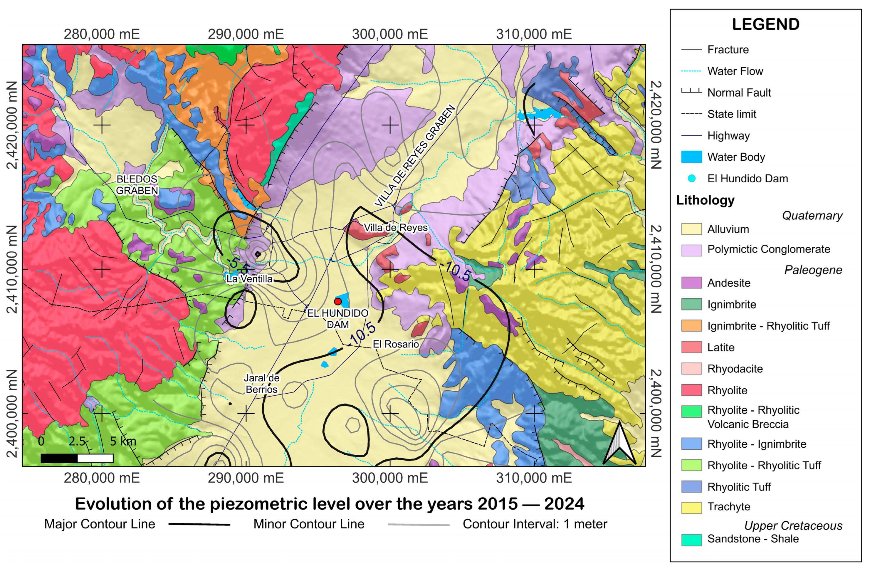
The El Hundido Dam is located at the southern part of the Villa de Reyes graben and south-east of the Bledos Semi-Graben. According to the geological map (Figure 2), this region is covered by pyroclastic flow deposits, lacustrine and alluvial sediments [25]. At the same time, the bedrock is composed of igneous rocks, especially rhyolites and ignimbrites, bounded by faults (Figure 2). The fault system that gave rise to the Villa de Reyes Graben was very active during the Early Oligocene and less active during the Late Oligocene, where it extended into the Early Miocene [26]. Currently, an active fault system is developing, with faults and fractures oriented NE-SW, which does not correspond to the N 30° system that gave rise to the Villa de Reyes Graben.
The effects of active faulting on the terrain and its relationship to aquifer recharge were supported by Perez-Martinez et al. [22]. Photographic evidence of active faulting at the study site was included in the Supplementary Materials.
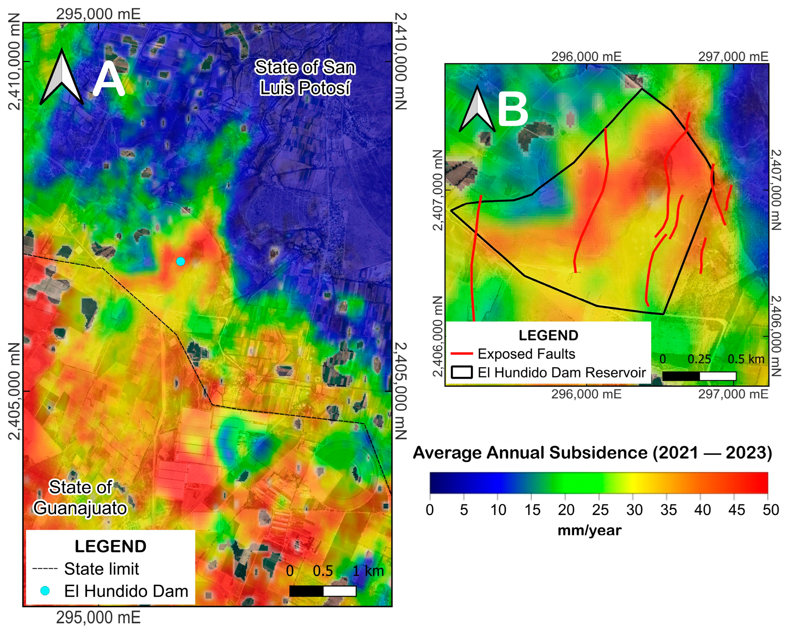
According to INEGI [31] data for 2021–2023, the study site is located on the northern edge of a significant subsidence zone (Figure 3A) within the Villa de Reyes graben, bordering the states of San Luis Potosí and Guanajuato.
Specifically, at the El Hundido Dam, the subsidence rate is variable, with the highest values of approximately 50 mm/year occurring in the central area of the former reservoir (Figure 3B). This area of higher subsidence includes zones with polygonal fracturing and fractures visible at the surface.
From a hydrogeological perspective, the area comprises a granular aquifer and a fractured aquifer. The upper granular aquifer is bounded by a clay unit 50 to 100 m thick. A thin layer of compact material with low hydraulic conductivity covers both the granular and fractured units in the valley. The granular aquifer ranges from 200 to 500 m thick, while the fractured aquifer can reach up to 400 m thick. At the valley’s edge, the piezometer reaches a depth of 120 m, whereas in the El Hundido area, it reaches approximately 64 m [32]. Groundwater flow originates from the mountainous areas and flows from southwest to northeast. From 2015 to 2024, the piezometric level at El Hundido Dam dropped by 9 m [30].

2. Materials and Methods

Three geoelectric methods were applied to characterise the subsoil in the study area. A TEM survey was conducted along a profile-oriented WSW-ESE line that crosses the dam to establish the stratigraphy of the sedimentary package in the subsoil and to characterise the topography of the igneous basement. The EMP method was applied to obtain apparent resistivity maps and to visualise lateral variations in electrical resistivity at different study depths. Finally, an ERT profile was carried out perpendicular to the fracture, with measurements taken for two electrode spacing, ensuring not only sufficient study depth but also high resolution in the shallowest part of the geoelectric section.

2.1. Transient Electromagnetic (TEM) Sounding

The transient electromagnetic (TEM) survey method is a time-domain controlled-source geoelectric technique [33]. The maximum depths that can be studied using the TEM method are in the order of hundreds of metres, depending on the electrical properties of the geological medium, the measurement time, and the dimensions of the cable loop. TEM sounding has been widely used in hydrogeological studies [34,35,36], in the delineation of saline intrusion [37,38,39], in mineral exploration [40,41,42], and in the modelling of bedrock [43,44,45].
A TerraTEM24 metre (Monex GeoScope, Melbourne, Victoria, Australia) [46], which has 12 data channels, and a single-wire loop were used for the TEM survey. The data logging was sampled simultaneously over the range 78 kHz to 625 kHz. A 150 × 150 m cable loop was used to reach a maximum study depth of 500 m.
The operating principle of the TEM method is as follows: a transmitter–receiver cable loop is placed on the ground surface, through which a short-pulse alternating current flows. The current induces an electromagnetic field in the geological medium, creating a secondary electromagnetic field that attenuates as it penetrates the subsoil. Once the source is turned off, the secondary electromagnetic field gradually attenuates, and the secondary fields detected by the receiver correspond to greater depths as the recording time elapses [47,48]. Therefore, it is possible to obtain an electromagnetic field decay curve and, subsequently, an apparent resistivity versus time (time after turning off the primary field) curve through a receiver wire loop [49].
The WinGLink software ver. 2.1.1 [50] was used to convert the apparent resistivity vs. time curve (experimental) into a 1-D geoelectric model. Using the “Edit” option, data affected by electromagnetic noise can be excluded (masked) from the inversion process. Additional information on the processing of TEM data is provided as Supplementary Materials. Initially, an automatic inversion and smoothing process comprising 18 layers was performed using the Nekut algorithm [51]. The generated multilayer model serves as the basis for a simplified 1-D model consisting of parallel, horizontal, and homogeneous layers. The theoretical apparent resistivity curve (the solution to the direct problem in geophysics) is calculated from the 1-D model. Next, the difference between the experimental and calculated curves is minimised until the standard root mean square error (RMSE) falls below 5%. Finally, the resulting 1-D model is considered as the solution to the inverse problem, obtained from a TEM survey.
In this work, twelve TEM soundings were carried out along profile (Figure 4A), with the main objective of modelling the topography of the igneous basement and determining whether geotectonic factors favour subsoil fracturing at the El Hundido Dam.

2.2. Electromagnetic Profiling (EMP) Method

When electrical measurements are taken at the surface of a homogeneous medium, the measured resistivity equals the medium’s actual electrical resistivity. In a heterogeneous medium, which is common in different geological environments, the resistivity measured at the surface includes contributions from all materials of different resistivities through which the electric or electromagnetic field flows and is called apparent resistivity (ρa).
EMP is a fast, non-contact method used to obtain apparent conductivity (σa) values in mS/m. The EMP method involves generating an EM field using a transmitter coil, inducing currents in the subsoil. These induced currents generate a secondary magnetic field. The apparent conductivity value can be calculated at a specific study depth from the relationship between the secondary and primary magnetic fields [52].
There are two ways to perform an EMP survey, depending on the orientation of the coils with respect to the ground surface: vertical dipole (VD) and horizontal dipole (HD). The VD mode consists of placing the R and T coils horizontally with respect to the ground surface. For the HD, both coils are placed vertically and aligned with the ground surface.
A CMD DUO metre (GF Instruments, Brno, Czech Republic) was used to perform the EMP survey. The CMD-DUO [53] consists of two coils, a receiver (R) and a transmitter (T), connected by a cable that defines their separation.
At the study site, all measurements were performed in VD mode and georeferenced.
The methodology applied for the fieldwork was as follows: three surveys were carried out, one using the 10 m cable, ensuring a maximum study depth of 15 m, on a 10 m × 10 m measurement grid, covering a total area of 0.33 km2 and 2185 measurement points. A second and third survey were carried out on a 40 m × 40 m measurement grid using 20 m and 40 m cables, ensuring maximum study depths of 30 m and 60 m, respectively, covering, in both cases, an approximate area of 0.63 km2 and a total of 15,850 measurement points. In all cases, σa (mS/m) values were converted to ρa (Ωm) values for mapping using the relationship ρa = 1000/σa.

2.3. Electrical Resistivity Tomography (ERT)

The ERT method applied along a profile allows a two-dimensional geoelectric model of subsoil resistivity distribution to be obtained, i.e., to determine variations in resistivity in both the vertical and horizontal directions [54], based on many ρa measurements taken on the ground surface. The method consists of inserting a set of equidistant electrodes into the ground along a profile, through which current will be injected and potential measured. The electrodes can be connected and disconnected either manually or automatically, the latter being achieved using smart or multi-core cables, which ensure greater efficiency. The ERT method is widely used in environmental [55], soil [56], archaeological [57], and groundwater [58] studies, as well as in the characterisation of active faults [59], among other applications.
For the ERT survey, a SuperSting R8 multi-electrode resistivity metre (Advanced Geosciences, Austin, Texas, United States of America) with multi-channel cables and 56 electrodes [60] was used to acquire ρa values automatically.
For any surface geophysical method, vertical resolution decreases with increasing study depth. For ERT, the spatial resolution depends on the electrode spacing. The smaller the electrode spacing, the higher the resolution. On the other hand, the study depth depends on the total distance covered by the electrode array.
Taking the above into account, two ERT data acquisition processes were designed along a single profile using the dipole–dipole array to obtain and compare geoelectric sections at different study depths and resolutions.
In the first (ERT1), a 10 m electrode spacing yielded a 56-electrode array 550 m long, ensuring a maximum study depth of 110 m. The ERT profile can be extended using the roll-along technique, which involves adding a section of smart cable with a limited number of electrodes, each of length 1/2 or 1/4 of the total array length [61]. A 275 m roll-along was then added, bringing the total ERT1 profile length to 825 m.
A second data acquisition process (ERT2) was carried out on the same profile with an electrode spacing of 3 m and an array length of 56 electrodes (165 m), which provided higher resolution and a shallower study depth (34 m). Eight roll-along lengths of 82.5 m were added for a total length of 825 m, equal to ERT1. For both ERT1 and ERT2, electrical contact between the electrode and ground was improved by adding saline solution, resulting in contact resistance (Rc) values below 1 KΩ in most connections. The SuperSting R8 was programmed to use the maximum output current of 2000 mA and a maximum voltage of 800 v.
The ERT study was conducted on an almost flat surface. According to the digital elevation model (see Figure 1C), the topographic variations. The ERT study was conducted on an almost flat surface. According to the digital elevation model (see Figure 1C), topographic variations along the profile were less than 2 m, so topographic corrections were not necessary for the geoelectric models derived from ERT1 and ERT2.
From the ERT survey, two apparent electrical resistivity sections are obtained and inverted to two electrical resistivity sections using Res2DInv, version 3.01 [62]. The Res2DInv software allows editing of apparent resistivity data collected in the field. Using the “exterminate bad datum points” option, it is possible to remove noisy data, primarily those affected by a high Rc value (>2.5 KΩ). In both ERT1 and ERT2, the removed ρa values did not exceed 3%.
The Res2DInv software uses an inversion routine based on Gauss–Newton least-squares methods with smoothness and finite-element constraints [63,64,65]. The robust inversion method was used to obtain better results in cases where the subsurface consists of homogeneous bodies that exhibit sharp contrasts with one another (e.g., igneous dykes or faults) [66]. To quantify the difference between the calculated and measured apparent resistivity, the root mean square (RMS) error was used, with convergence achieved in at most 6 iterations. An RMS error of 9.7% was obtained for ERT1, while ERT2 had an RMS error of 3.6%. The main inversion settings are presented in the Supplementary Materials. After inversion, the data were plotted in Surfer 16.3. [67] to improve the image quality of both ERT profiles.

3. Results

3.1. TEM Results

3.1.1. Geoelectrical Section

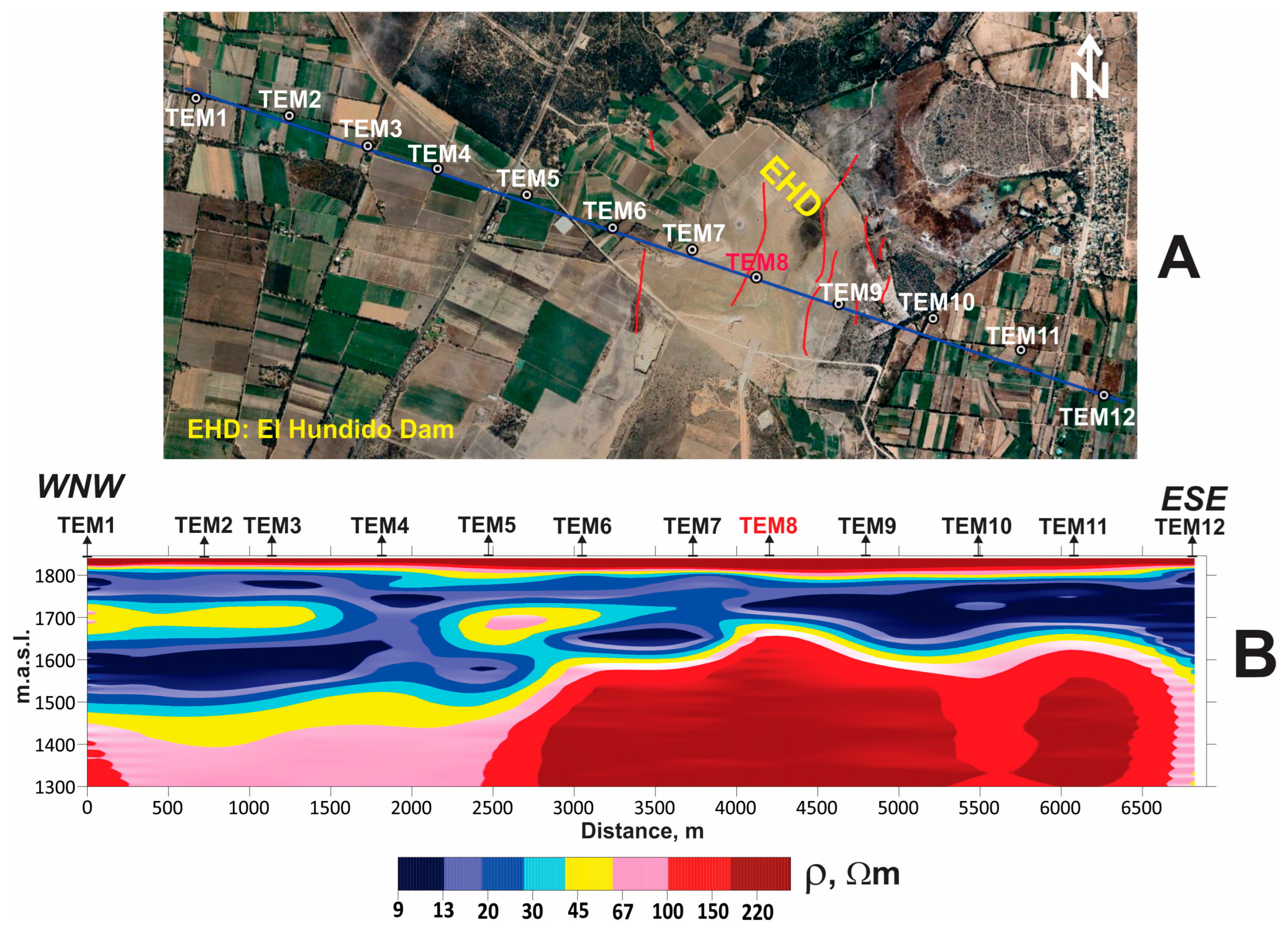
The TEM profile, with a length of 6800 m and a WNW-ESE orientation, includes 12 soundings (TEM 1 to TEM12), with TEM8 located in the centre of the El Hundido Dam (Figure 4A).
Figure 4B shows the geoelectric section resulting from the interpolation of the twelve 1-D models obtained from the TEM survey carried out in profile. In general, three geoelectric units are observed. A first resistive layer (ρ > 65 Ωm, Figure 4B) with a variable thickness between 30 m and 60 m corresponds to the dry and friable alluvial material observed on the ground surface and into fractures. This first unit is underlain by a second conductive unit with a resistivity ranging from 9 to 55 Ωm (Figure 4B). Based on the piezometric level maps of the region, this unit must include the local aquifer, so increased moisture leads to lower resistivity values. Finally, there is a resistive (ρ > 65 Ωm, Figure 4B) bedrock (third unit). The depth to the top of the bedrock is highly variable; for the 3000–6500 m interval of the profile, the bedrock rises, reaching a minimum depth of 140 m for TEM8, where resistivity values are greater than 100 Ωm (Figure 4B). For the first 2500 m of the profile, the depth to the bedrock increases, reaching a maximum of 450 m in TEM2, where electrical resistivity values decrease (ρ ~ 70 Ωm, Figure 4B).

3.1.2. 1D Geological-Geoelectric Model of a Dam Reservoir

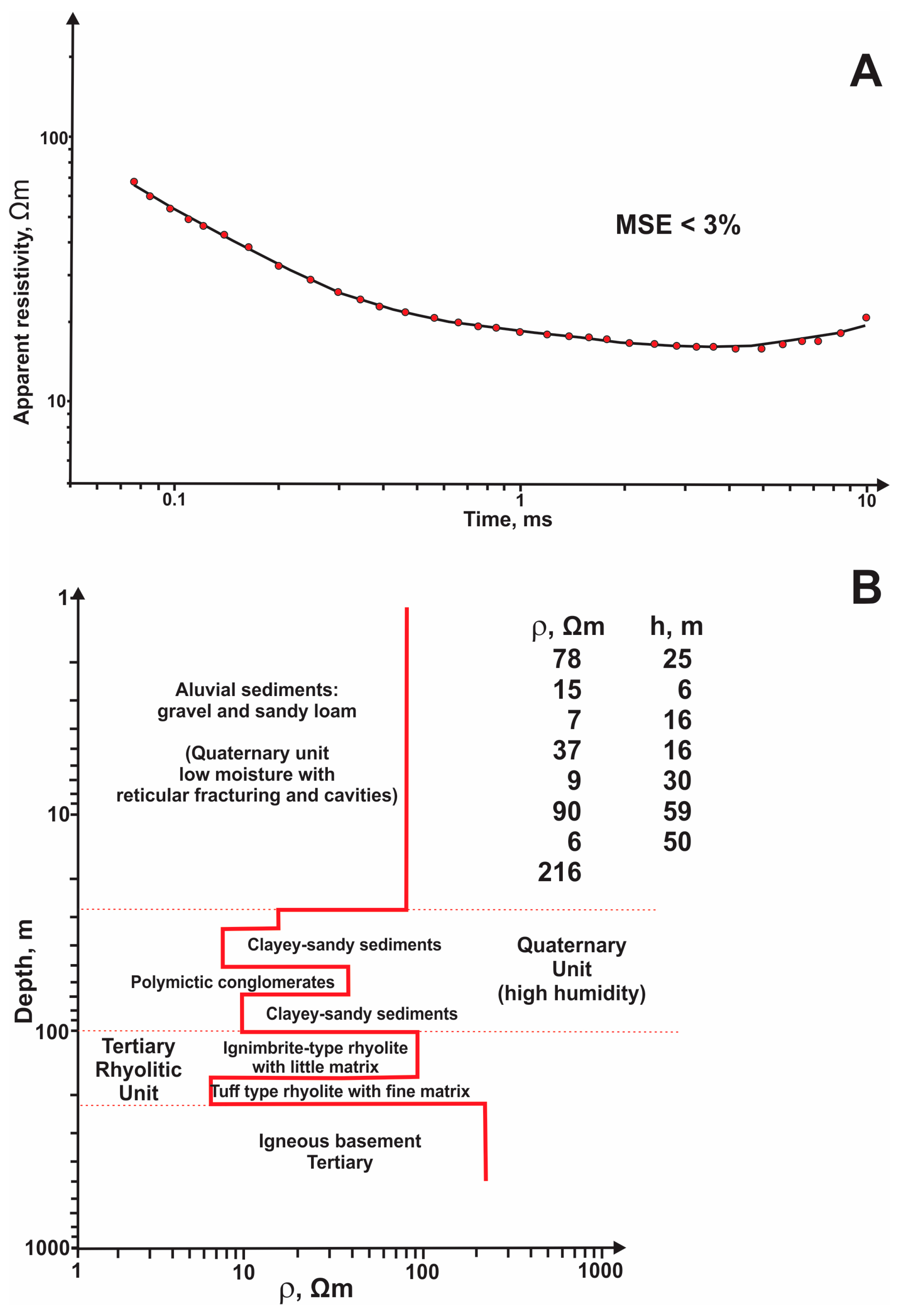
To provide an overview of the subsoil lithological composition in the dam reservoir, the 1D model from the TEM8 sounding is shown in Figure 4.
In Figure 5A, the ρa curve of observed data is shown as red dots, while the solid line corresponds to the calculated ρa curve for the 1D model, presented in Figure 5B. The root mean square error (RMSE) between the two curves is less than 3%, according to the parameters provided by the WingLink software ver. 2.1.1 [50].
According to the outcrops and geological map of the area (SGM [27], Figure 2), the first layer, ρ = 78 Ωm and 25 m thick (Figure 5B), corresponds to Quaternary alluvium composed of gravels and sandy–loamy sediments. This first layer, very dry at the time of the TEM study, with numerous fractures and sunken cavities, exhibits a high resistivity value due to its low moisture content and friability. These conditions favour hydro-compaction due to rainwater infiltration into the soil structure, which redistributes particles and, consequently, modifies their volume, causing subsidence.
Underlying the resistant surficial unit, there is a second group of conductive layers composed of clayey–sandy sediments and Quaternary polymictic conglomerates, which outcrop on the slopes of the Sierra de San Miguelito (Figure 2). The increased clay content in the sediments and the gradual increase in moisture, reaching saturation at depths greater than 64 m, are reflected in resistivity values below 10 Ωm for the clayey–sandy sediments, while for the conglomerates the value is slightly below 40 Ωm. This high-moisture Quaternary unit reaches a thickness of 68 m (Figure 5B).
A third Tertiary rhyolitic unit underlies the Quaternary conglomerates and sediments, with a total thickness of approximately 109 m. According to the geological outcrop map (Figure 2), this unit is in the areas adjacent to the Sierra de San Miguelito. It is divided into two subunits: an upper resistive subunit and a lower conductive subunit. This behaviour is typical of the Panalillo Rhyolite, which has two members [28]: an upper member formed by well-welded ignimbrites with little matrix (more permeable and resistive, with ρ = 90 Ωm, Figure 5B) and a lower member of fragmented tuff with fine-grained sediments (less permeable and more conductive, with ρ = 6 Ωm, Figure 5B).
Finally, we have a basement of igneous rocks, whose resistivity corresponds to the Portezuelo Latite, where variable resistivities between 51 and 500 Ωm have been reported, depending on the degree of alteration and fracturing [29]; at the study site, it reaches a value of approximately 216 Ωm (Figure 5B).
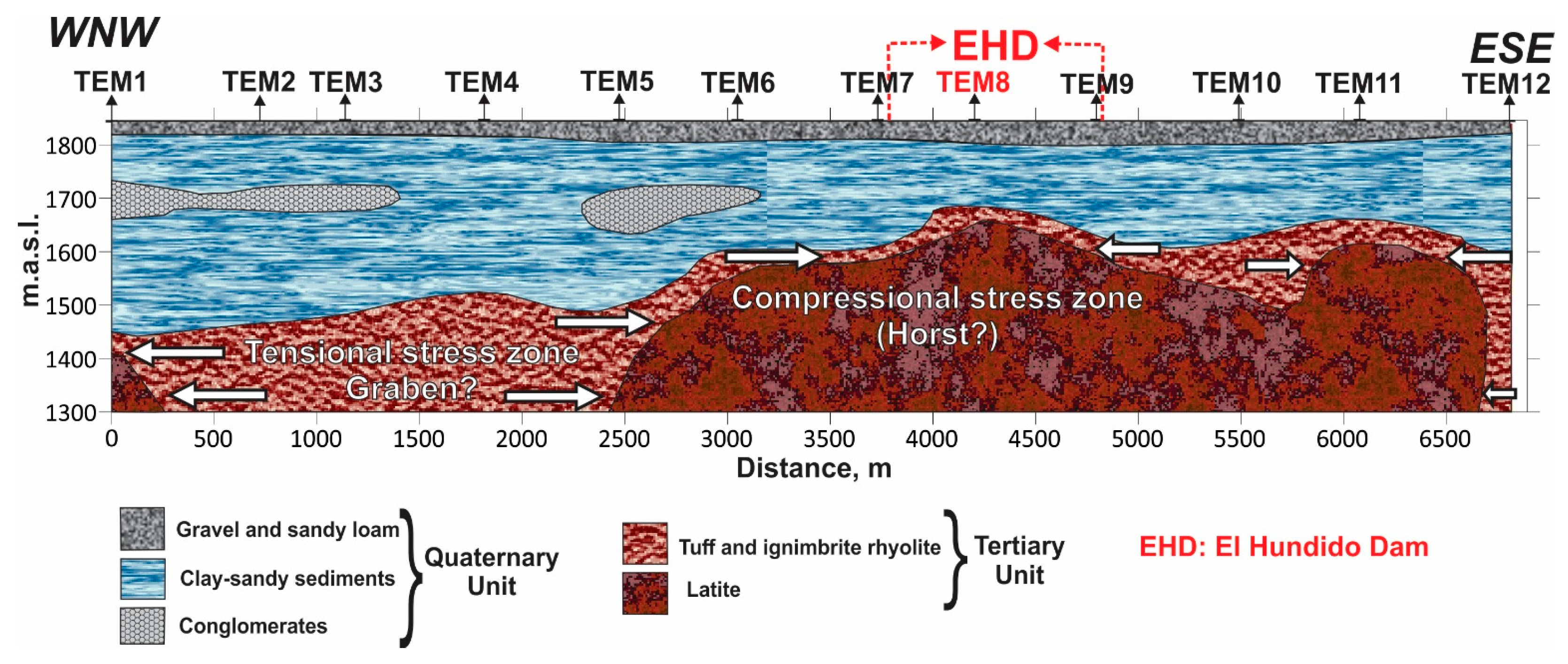
Based on the geological interpretation of the TEM8 geoelectric model (centre of the El Hundido Dam, Figure 5B), the geoelectric section of the TEM profile (Figure 4B) was converted into the geological section shown in Figure 6. Noteworthy is the topography of the igneous basement (Tertiary unit) in the interval between 2450 m and 6600 m, where the latite rises in what appears to be a horst, descending to a depth greater than 550 m in the interval between 250 m and 2450 m, forming a graben filled with rhyolitic material (Figure 6).

3.2. EMP Survey

The resistivity data resulting from each EMP survey were processed and converted into ρa maps using Surfer 16.6 software [67].
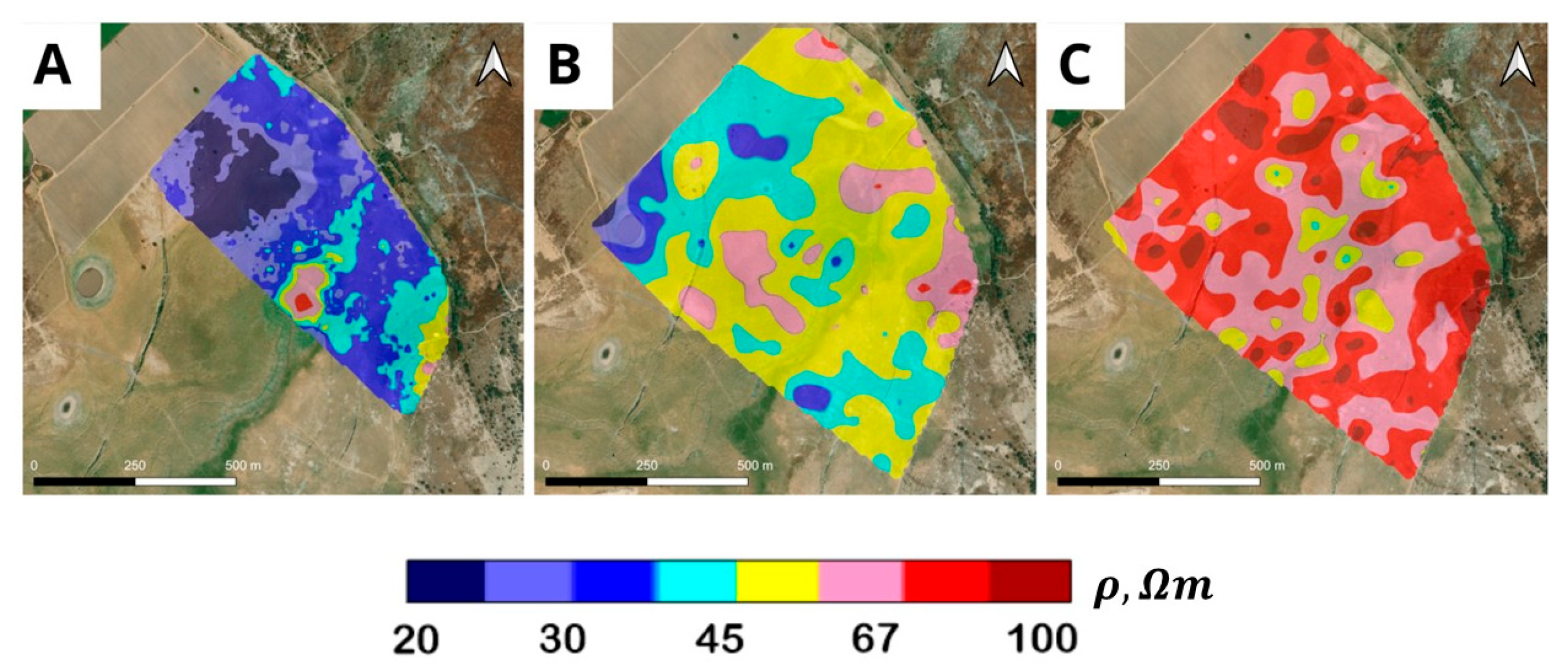
Figure 7 shows the ρa maps for the maximum study depths of 15 m, 30 m, and 60 m. The map in Figure 7A shows the geoelectric behaviour of the shallowest part of the subsurface. A low-resistivity anomaly (ρa < 30 Ωm) stands out in the northwest, indicating the possible presence of clayey material and coinciding with the absence of surface fractures in the terrain.
Toward the south–southeast, ρa values increase, evidencing the absence of clayey material and the presence of fractures and sunken holes. In the south-central part of the map, along the polygonal fracture zone, a small high-resistivity anomaly is observed, indicating the presence of dry, friable material with abundant voids.
The second map shows the lateral variations of ρa up to a maximum study depth of 30 m. In Figure 7B, neither the low-resistivity anomaly associated with the clayey material nor the high-resistivity anomaly associated with the polygonal fracturing zone can be observed, which limits the presence of both to depths below 20 m. In general, the map shows a more uniform environment, with most resistivity values ranging from 30 to 60 Ωm; increased humidity with depth can reduce resistivity contrasts.
Figure 7C shows the third and final ρa map corresponding to a maximum study depth of 60 m. In general, ρa values show a significant increase. The values of ρa are mostly in the range of 37 to 90 Ωm. This increase may be due to the influence of polymictic conglomerates. CONAGUA [68] reported static levels for the region with minima of 64 m in the El Hundido area, so these conglomerates are considered to comprise the local aquifer.

3.3. ERT Results

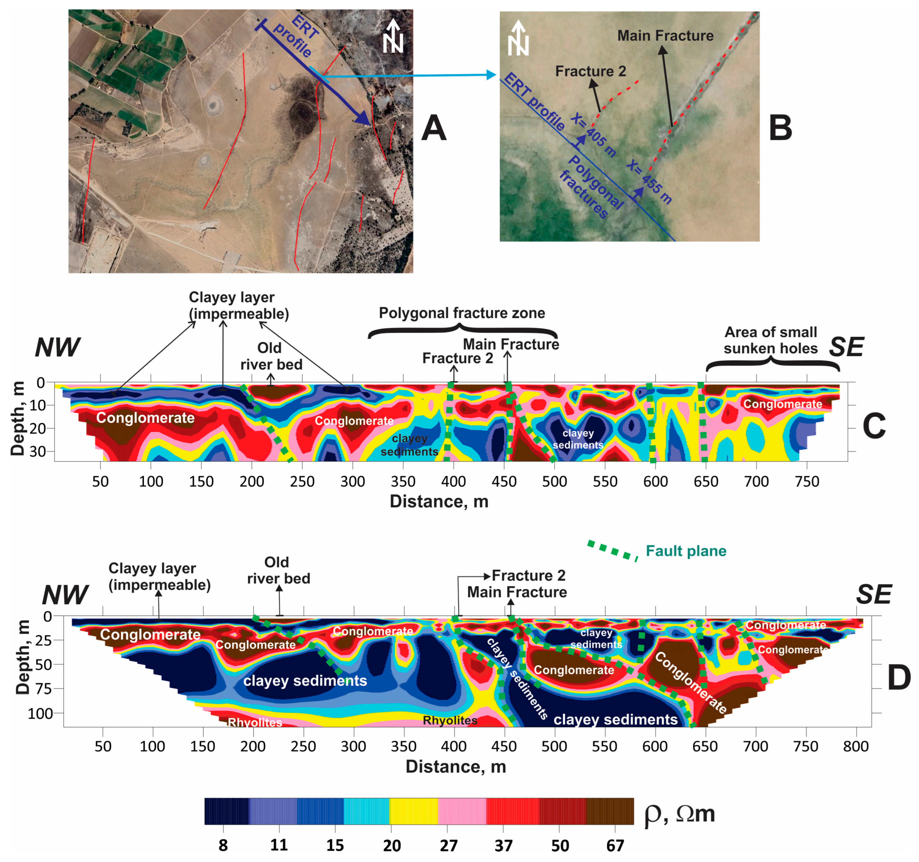
Although the TEM survey results provided information on the topography of the tertiary basement, the 1-D models obtained cannot model fractures. To model faults and fractures, a 2-D inversion is necessary. Therefore, an ERT profile was surveyed in a NW-SE direction (Figure 8A) so that it would intersect perpendicularly one of the visible fractures (hereinafter “the main fracture”) in the dam reservoir (Figure 8B). The first ERT profile was performed with an electrode spacing of 3 m to obtain a high-resolution model for the first 34 m depth. A second profile, coincident with the first, is performed with 10 m electrode spacing to obtain a medium-resolution model reaching 110 m depth, exceeding the saturation levels in the subsoil.
  • Geoelectrical section for 34 m study depth (high resolution)
A conductive surface layer (ρ = 6–16 Ωm) approximately 6–7 m thick is observed in the first 325 m of the profile (Figure 8C). This layer occupies a large part of the northern portion of the dam reservoir. It is the cause of the conductive anomalies described in the ρa map for the study depth of 15 m (Figure 7A). This layer, which outcrops in some areas of the dam reservoir with high clay content, appears discontinuously and with less thickness in the last 200 m of the profile (Figure 8C). This clayey layer acted as a barrier to surface water infiltration, allowing it to be stored in the dam reservoir. In the central part of the profile, between 325 m and 575 m, the clay layer disappears, coinciding with the area where the terrain is most affected by small and large fractures, as well as sunken holes, in addition to being crossed by the main fracture (Figure 8B). The absence of this impermeable layer in the central part of the reservoir makes it impossible to retain rainwater, which infiltrates quickly, aided by the fractures in the terrain.
Other notable features of the high-resolution profile include the cross-sectional view of the former streambed that fed the reservoir (now permanently dry) (Figure 8C). This riverbed appears as a marked resistive anomaly due to its fill composed of gravel and sand of different grain sizes. In the last 175 m of the profile, a surface layer with an average thickness of 3 m stands out as a resistive anomaly (ρ > 55 Ωm, Figure 8C), corresponding to the area where several small sunken holes appear.
Finally, one of the most important aspects of the section is the modelling of the main fracture (Figure 8B,C). The fracture plane shows an area of high resistivity due to the presence of friable, dry material with a predominance of voids, where hydro-compaction is favoured and the highest subsidence rates are observed (Figure 3).
  • Geoelectrical section for 110 m study depth (medium resolution)
The second profile (ERT2) was carried out coinciding with the first (ERT1), but with a 10 m electrode separation, reaching a maximum study depth of 110 m. The 2D model presented in Figure 8D was fed back into its first 34 m with information from the first model (ERT1) shown in Figure 8C.
A notable feature is a reverse geological fault associated with the two fractures modelled in the high-resolution model (ERT1). The fault, bounded by the two fractures, is in the interval 405 m and 470 m, with the hanging-wall block to the NW and the foot-wall block to the SE (Figure 8D). The presence of a reverse fault is characteristic of a positive flower-type fracture system. On the left side of the “fracture 2” (<400 m), the stratigraphy corresponds to that described in the TEM8 model, where the Quaternary unit reaches a depth of 100 m, below which the resistive rhyolite ignimbrites appear (Figure 8D). On the right side of the main fracture (>460 m, Figure 8D)), the stratigraphy changes, becoming more chaotic, showing resistive bodies (ρ > 60 Ωm) corresponding to the rhyolite ignimbrites starting at a depth of 30–40 m. In the 400–460 m interval of the profile, a wide fault plane is characterised by low resistivity values (ρ < 10 Ωm), caused by the migration and accumulation of fine, moist sediments across the fracture, especially during the rainy season. The main fracture is at a depth greater than 100 m, below the water table (64 m), which rules out an anthropogenic origin; otherwise, faulting would occur only in the surface layers at depths shallower than 64 m.
In the tomographic profile at an exploration depth of 110 m (Figure 8D), thick packages of sedimentary material (sands, silts, and clays) predominate, interrupted by more resistant materials consisting of sand and conglomerates (ρ > 20 Ωm). In the central part of the profile, a thinning of the conglomerate layer and slight deformation of the underlying sandy–clayey material (ρ < 20 Ωm) are visible. The presence of fractures interrupts these sedimentary bodies in the surface and central portions of the profile.

4. Discussion

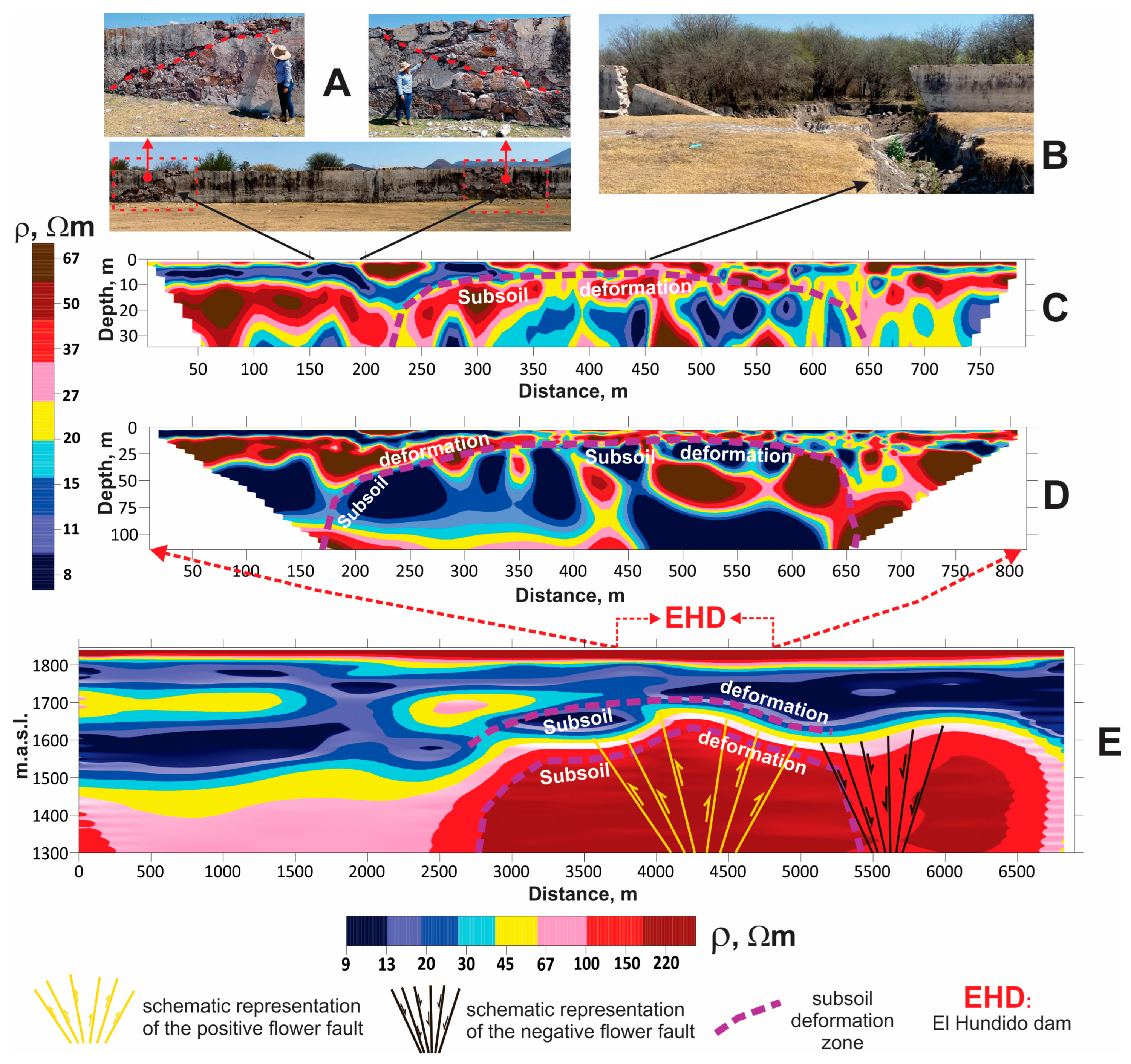
Figure 9 shows the geoelectric sections obtained at different study depths, along with surface evidence of compressive stress (Figure 9A) and active faulting (Figure 9B).
As mentioned previously, the geoelectric section obtained from the TEM study, derived from correlations among the twelve one-dimensional models (Figure 9E), while not permitting modelling of a fracture plane, generally shows the convex topography of the igneous basement (latite).
The ERT2 geoelectric section (medium resolution, Figure 9D) shows a distribution of deformed conglomerate material in the central part of the profile (central part of the dam), interrupted by sedimentary material with lower resistivity associated with fractures. In the deformation zone, there are fractures (such as the main fracture, Figure 8) that extend deep into the ground beyond the saturation zone of the subsoil (~64 m) (Figure 9D). Consequently, large fractures (such as the main fracture, Figure 9B) oriented NNE-SSW are geological faults rather than surface fractures. At higher resolution, the ERT1 geoelectric section (Figure 9C) provides a more detailed representation of subsurface deformation caused by bedrock uplift in the 200–600 m section of the profile. At higher resolution, the ERT1 geoelectric cross-section (Figure 9C) provides a more detailed representation of subsurface deformation caused by bedrock uplift in the 200 m to 600 m interval of the profile. In the northwestern section of the dam, EMP (Figure 7A) and ERT (Figure 8C,D) studies show the presence of a clayey (impermeable) surface layer that was essential for water storage in the reservoir. Currently, this layer has been destroyed across most of the dam.
Therefore, it can be concluded that there is a natural conditioning factor (local tectonics) for the subsurface faulting. Active faulting, combined with the drop in the water table (anthropogenic cause), favours polygonal faulting and hydro-compaction processes (subsidence) in the surface alluvial sediments, primarily in the central area of the dam. The subsurface deformation is expressed at the surface in the dam wall (Figure 9A,B), confirming the shallower structures described by Monge-Cerda et al. [19].
Similar results were obtained by Villaseñor-Reyes et al. [16] in the city of Zamora, Michoacán, where the PSI technique was applied for the period 2014–2021, delimiting areas with subsidence rates between 102 and 108 mm/year, while the results of applying TEM sounding made it possible to define a model of the bedrock, including the presence of graben, semi-graben and horst, that tectonically condition subsidence in the city.
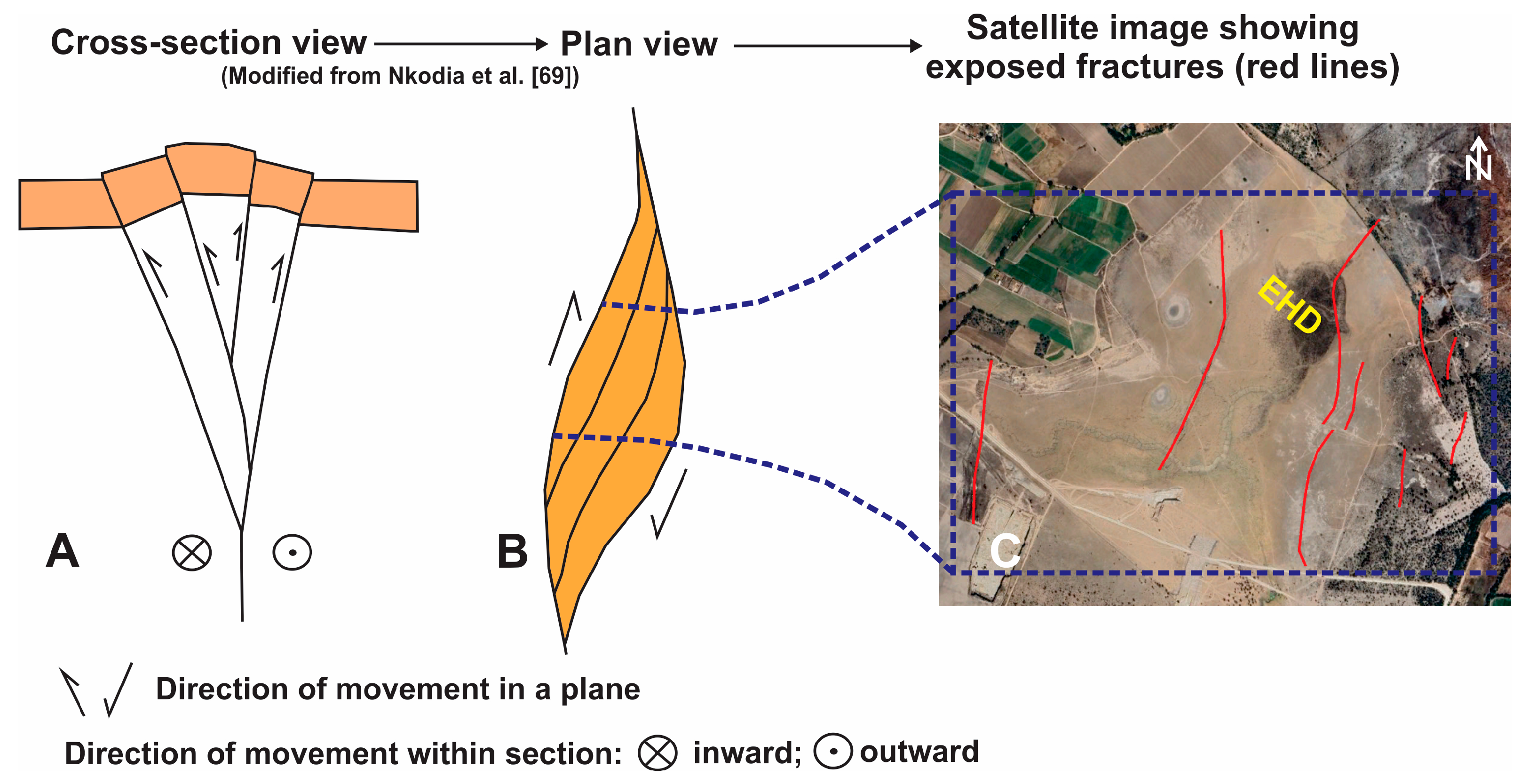
The uplift of the igneous bedrock in the dam area (Figure 9E) is caused by transcompressive stresses that generate subsurface deformations within a fault system, corresponding to the positive flower pattern described by Nkodia et al. [69]. Flower-type faults appear in cross-section as a system of fractures that branch out at depth from a common trunk and diverge upwards (see Figure 10A). When the fracture zone has a convex geometry, it is referred to as a “positive flower” [69]. In the El Hundido Dam zone, the TEM survey results obtained in this study show a Tertiary igneous basement with deformations typical of compressive stress (Figure 6), which are the conditioning factor in the site’s faulting, specifically positive flower faults (Figure 10A).
The convex geometry of the igneous basement is not clearly visible on the surface (except in the dam wall) due to the thickness (~100 m) of the Quaternary unit and the differential compaction that has occurred in the dam basin caused by the accelerated decline of the piezometric level. However, the visible faults (Figure 10C), with a predominant SSW-NNE orientation, correspond to the plan view of the positive flower-type fault system (Figure 10B) described by Nkodia et al. [69]. The extent of these surface fractures cannot be determined because agricultural activity obscures them.

5. Conclusions

This integrated geoelectric study of the El Hundido Dam provides strong evidence that surface deformations and fracturing are controlled by deep, active tectonic activity.
TEM results delineate a volcanic basement with a convex morphology, interpreted as a horst bounded by reverse faults. ERT images confirm the presence of fault structures and macrostructures that cut and deform the overlying materials. The integration of different profiles at various resolution levels reveals a positive flower-type fault system generated by compressive and transpressional stresses.
While local tectonics is a conditioning factor in the formation of geological faults, the overexploitation of groundwater and the drop in the water table magnify the phenomenon and contribute to the formation of polygonal surface cracking, hydro-compaction-induced subsidence, and sunken holes.
The results of this study highlight the importance of integrating geophysical methods at multiple resolution levels to distinguish anthropogenic from tectonic factors in areas with active faulting. This distinction is important for risk assessment, urban development planning, and land use management in tectonically active basins. The methodological approach of this work is transferable to other regions with similar tectonically active basins worldwide.
Future work should incorporate other methods, such as high-resolution seismic and magnetotelluric surveys, to better define the geometry of tectonic structures at depth and, using InSAR techniques, to monitor and quantify the rate of ground deformation.

Supplementary Materials

The following supporting information can be downloaded at: https://www.mdpi.com/article/10.3390/geosciences16060209/s1, Figure S1: locations of the points where photographs of the fractures were taken and their effects on the dam’s infrastructure; Figure S2: Photographs of the fissures and their effects on the dam wall; Figure S3: Changes in piezometric levels for the 2015–2024 period in the region that includes the El Hundido Dam; Figure S4: (A) Photograph of the central part of the dam showing evidence of polygonal fracturing and a larger sunken hole. (B) Close-up view of the polygonal fracturing. (C) Photo of a small sunken hole; Figure S5: Display of the Terra TEM24 meter; Table S1: Main inversion settings using the Res2DInv software.

Author Contributions

X.M.T.-M. and O.D.-R.: Conceptualisation, methodology, investigation and writing—original draft preparation. J.A.R.-L., H.J.P.-G. and S.E.C.-L.: Formal analysis, supervision and writing—review and editing. All authors have read and agreed to the published version of the manuscript.

Funding

This research received no external funding.

Data Availability Statement

The data used in this work are available upon request from the corresponding author.

Acknowledgments

This work was supported by grants from the Instituto Potosino de Investigación Científica y Tecnológica A.C. (IPICYT) and by the Secretaría de Ciencia, Humanidades, Tecnología e Innovación (SECIHTI). The authors would like to thank Ángel Frías García, director of Gogorrón National Park, for serving as a liaison between us and the communal landowners. Special thanks to David Ernesto Torres-Gaytán for their fieldwork assistance.

Conflicts of Interest

The authors declare no conflicts of interest.

References

  1. Davydzenka, T.; Tahmasebi, P.; Shokri, N. Unveiling the Global Extent of Land Subsidence: The Sinking Crisis. Geophys. Res. Lett. 2024, 51, e2023GL104497. [Google Scholar] [CrossRef] [Scilit]
  2. Devi, A.; Moisio, S. How ‘Sinking Cities’ Can Address Subsidence Challenges. World Economic Forum. Available online: https://www.weforum.org/stories/2024/10/how-sinking-cities-can-address-subsidence-challenges/ (accessed on 25 March 2026).
  3. Brunori, C.A.; Bignami, C.; Albano, M.; Zucca, F.; Samsonov, S.; Groppelli, G.; Norini, G.; Saroli, M.; Stramondo, S. Land subsidence, Ground Fissures and Buried Faults: InSAR Monitoring of Ciudad Guzmán (Jalisco, Mexico). Remote Sens. 2015, 7, 8610–8630. [Google Scholar] [CrossRef] [Scilit]
  4. Zisman, E.D.; West, S.D. Hydrocompaction Considerations in Sinkhole Investigations. NCKRI Symp. 2015, 5, 605–611. [Google Scholar] [CrossRef] [Scilit]
  5. Zumpano, V.; Pisano, L.; Parise, M. An integrated framework to identify and analyze karst sinkholes. Geomorphology 2019, 332, 213–225. [Google Scholar] [CrossRef] [Scilit]
  6. Bagheri-Gavkosh, M.; Mossa-Hosseini, S.; Ataie-Ashtiani, B.; Sohani, Y.; Ebrahimian, H.; Morovat, F.; Ashrafi, S. Land subsidence: A global challenge. Sci. Total Environ. 2021, 778, 146193. [Google Scholar] [CrossRef] [Scilit]
  7. Raspini, F.; Caleca, F.; Del Soldato, M.; Festa, D.; Confuorto, P.; Bianchini, S. Review of satellite radar interferometry for subsidence analysis. Earth-Sci. Rev. 2022, 235, 104239. [Google Scholar] [CrossRef] [Scilit]
  8. Castellazzi, P.; Arroyo-Domínguez, N.; Martel, R.; Calderhead, A.I.; Normand, J.C.L.; Gárfias, J.; Rivera, A. Land subsidence in major cities of Central Mexico: Interpreting InSAR-derived land subsidence mapping with hydrogeological data. Int. J. Appl. Earth Obs. Geoinf. 2016, 47, 102–111. [Google Scholar] [CrossRef] [Scilit]
  9. Chaussard, E.; Amelung, F.; Wdowinski, S.; Cabral-Cano, E. Magnitude and extent of land subsidence in central Mexico revealed by regional InSAR ALOS time-series survey. Geophys. Res. Abstr. 2013, 15, EGU2013-4841. [Google Scholar]
  10. Figueroa-Miranda, S.; Hernández-Madrigal, V.; Tuxpan-Vargas, J. Evolution assessment of structurally-controlled differential subsidence using SBAS and PS interferometry in an emblematic case in Central Mexico. Eng. Geol. 2020, 279, 105860. [Google Scholar] [CrossRef] [Scilit]
  11. Cigna, F.; Tapete, D. Present-day land subsidence rates, surface faulting hazard and risk in Mexico City with 2014–2020 Sentinel-1 IW InSAR. Remote Sens. Environ. 2021, 253, 112161. [Google Scholar] [CrossRef] [Scilit]
  12. Chaussard, E.; Havazli, E.; Fattahi, H.; Cabral-Cano, E.; Solano-Rojas, D. Over a century of sinking in Mexico City: No hope for significant elevation and storage capacity recovery. J. Geophys. Res. Solid Earth 2021, 126, e2020JB020648. [Google Scholar] [CrossRef] [Scilit]
  13. Navarro-Hernández, M.I.; Tomás, R.; Lopez-Sanchez, J.M.; Cárdenas-Tristán, A.; Mallorquí, J.J. Spatial Analysis of Land Subsidence in the San Luis Potosi Valley Induced by Aquifer Overexploitation Using the Coherent Pixels Technique (CPT) and Sentinel-1 InSAR Observation. Remote Sens. 2020, 12, 3822. [Google Scholar] [CrossRef] [Scilit]
  14. Zapata-Norberto, B.; Morales-Casique, E.; Contreras-Galván, R.; Ramos-Leal, J.A. Land subsidence in Mexico City: New insights from field data and numerical modeling. Groundw. Sustain. Dev. 2025, 29, 101432. [Google Scholar] [CrossRef] [Scilit]
  15. Dindi, E. An assessment of the performance of the geophysical methods as a tool for the detection of zones of potential subsidence in the area southwest of Nakuru town, Kenya. Environ. Earth Sci. 2015, 73, 3643–3653. [Google Scholar] [CrossRef] [Scilit]
  16. Villaseñor-Reyes, C.I.; Hernández-Madrigal, V.M.; Delgado-Rodríguez, O.; Guevara-Alday, J.A.; Flores-Lázaro, N. 3D deformation velocity field analysis and TEM method to detect the tectonic influence on the land subsidence in Zamora, Mexico. Eng. Geol. 2024, 338, 107636. [Google Scholar] [CrossRef] [Scilit]
  17. Pacheco, J.; Arzate, J.; Rojas, E.; Arroyo, M.; Yutsis, V.; Ochoa, G. Delimitation of ground failure zones due to land subsidence using gravity data and finite element modeling in the Queretaro valley, Mexico. Eng. Geol. 2006, 84, 143–160. [Google Scholar] [CrossRef] [Scilit]
  18. Wang, P.; Li, F.; Lu, K.; Huang, W. Detection of water-rich areas and seepage channels via the transient electromagnetic method, electrical resistivity tomography, and self-potential method. Sci. Rep. 2025, 15, 15905. [Google Scholar] [CrossRef] [Scilit] [PubMed]
  19. Monge-Cerda, F.; Ramos-Leal, J.; Delgado-Rodríguez, O.; Torres-Hernández, J.; Belmonte-Jiménez, S.; Torres-Gaytán, D. Geophysical, geological and tectonic study of active faulting inside the Villa de Reyes Graben, Central México. Near Surf. Geophys. 2025, 23, 460–482. [Google Scholar] [CrossRef] [Scilit]
  20. CONAGUA. Informe de Inspección a la Presa San Francisco en el Municipio de Villa De Reyes; Subgerencia de Seguridad de Presas; S.L.P. Gerencia Estatal En San Luis Potosí: San Luis Potosí, Mexico, 2000; Volume 3093, p. 7. [Google Scholar]
  21. Murillo, R. Presas de Tierra y sus Fallas. XXVI Reunión Nacional de Mecánica de Suelos e Ingeniería Geotécnica. Sociedad Mexicana de Ingeniería Geotécnica, A.C. Cancún, Quintana Roo, México. 2012. Available online: https://www.studocu.com/pe/document/universidad-cesar-vallejo/obras-hidraulicas/presas-de-tierra-y-sus-fallas/83484880 (accessed on 18 March 2026).
  22. Pérez-Martínez, I.; Ramos-Leal, J.A.; Cardona-Benavides, A.; Morán-Ramírez, J.; Villanueva-Estrada, R.E. Caracterización hidrogeoquímica para la identificación y cuantificación de los flujos que dan origen al agua subterránea en un valle tectónico. Environ. Earth Sci. 2021, 80, 772. [Google Scholar] [CrossRef] [Scilit]
  23. Gutiérrez, F.; Guerrero, J.; Lucha, P. A genetic classification of sinkholes illustrated from evaporite paleokarst exposures in Spain. Environ. Geol. 2008, 53, 993–1006. [Google Scholar] [CrossRef] [Scilit]
  24. Fannin, R.; Slangen, P. On the distinct phenomena of suffusion and suffosion. Géotechnique Lett. 2014, 4, 289–294. [Google Scholar] [CrossRef] [Scilit]
  25. Tristán-González, M. Estratigrafía y Tectónica del Graben de Villa de Reyes, en los Estados de San Luis Potosí y Guanajuato; Universidad Autónoma de San Luis Potosí, Instituto de Geología: San Luis Potosí, Mexico, 1986; Volume 107, p. 91. [Google Scholar]
  26. Nieto-Samaniego, Á.F.; Alaniz-Álvarez, S.A.; Labarthe-Hernández, G. La deformación cenozoica poslaramídica en la parte meridional de la Mesa Central, México. Rev. Mex. Cienc. Geológicas 1997, 14, 13–25. [Google Scholar]
  27. SGM. Carta Geológico-Minera, Santa María del Río F14-C14, San Luis Potosí y Guanajuato [Map]. Secretaría de Economía. 1997. Available online: http://mapserver.sgm.gob.mx/Cartas_Online/geologia/1462_F14-C14_GM.pdf (accessed on 25 March 2026).
  28. Labarthe-Hernández, G.; Tristán-González, M.; Aranda-Gómez, J.J. Revisión Estratigráfica del Cenozoico de la Parte Central del Estado de San Luis Potosí; Universidad Autónoma de San Luis Potosí, Instituto de Geología y Metalurgia: San Luis Potosí, Mexico, 1982; p. 85. [Google Scholar]
  29. Ramos-Leal, J.; López-Loera, H.; Martínez-Ruiz, V.; Aranda-Gómez, J. Sucesión de eventos y geometría de la parte central del acuífero del graben de Villa de Reyes (San Luis Potosí, México) inferida a partir de datos geoeléctricos. Rev. Mex. Cienc. Geológicas 2007, 24, 31–46. [Google Scholar]
  30. CONAGUA. Consulta De Mediciones Piezométricas. Gerencia De Aguas Subterráneas. 2024. Available online: https://sigagis.conagua.gob.mx/rp20/ (accessed on 20 April 2026).
  31. INEGI. Distribución Espacial y Magnitud de la Subsidencia en Villa de Reyes, San Luis Potosí en 2022. 2024. Available online: https://www.inegi.org.mx/app/biblioteca/ficha.html?upc=794551118177 (accessed on 20 April 2026).
  32. Hernández Bocanegra, P.I. Exploración Geofísica e Hidrogeoquímica en el Graben de Villa de Reyes, Para Estudiar el Origen de las Fallas Activas y sus Implicaciones en el Acuífero. Master’s Thesis, Instituto Potosino de Investigación Científica y Tecnológica, San Luis Potosí, Mexico, 2023. Available online: http://hdl.handle.net/11627/6463 (accessed on 17 March 2026).
  33. Telford, W.M.; Geldart, L.P.; Sheriff, R.E. Resistivity Methods. In Applied Geophysics, 2nd ed.; Cambridge University Press: Cambridge, UK, 1990; pp. 353–358. [Google Scholar] [CrossRef] [Scilit]
  34. McLachlan, P.; Vang, M.Ø.; Pedersen, J.B.; Kraghede, R.; Christiansen, A.V. Mapping the Hydrogeological Structure of a Small Danish Island Using Transient Electromagnetic Methods. Groundwater 2025, 63, 280–290. [Google Scholar] [CrossRef] [Scilit]
  35. Lévesque, Y.; Walter, J.; Chesnaux, R. Transient Electromagnetic (TEM) Surveys as a First Approach for Characterizing a Regional Aquifer: The Case of the Saint-Narcisse Moraine, Quebec, Canada. Geosciences 2021, 11, 415. [Google Scholar] [CrossRef] [Scilit]
  36. Zhang, Y.; Wu, Y.; Zheng, H.; Xu, Y.; Cheng, X. Application of TEM and HDRM in hydrogeophysical surveys in Meisibulake coal mine. Sci. Rep. 2022, 12, 21368. [Google Scholar] [CrossRef] [Scilit]
  37. Rajab, J.A.; Yogeshwar, P.; Tezkan, B. Transient electromagnetic imaging of saltwater intrusion at the shrinking Dead Sea. Sci. Rep. 2025, 15, 30250. [Google Scholar] [CrossRef] [Scilit] [PubMed]
  38. Zhu, Z.; Shan, Z.; Pang, Y.; Wang, W.; Chen, M.; Li, G.; Sun, H.; Revil, A. The transient electromagnetic (TEM) method reveals the role of tectonic faults in seawater intrusion at Zhoushan islands (Hangzhou Bay, China). Eng. Geol. 2024, 330, 107425. [Google Scholar] [CrossRef] [Scilit]
  39. Zamora-Luria, J.C.; McLachlan, P.; Christiansen, A.V. Long-term monitoring of water table and saltwater intrusion dynamics through time-lapse transient electromagnetic. Near Surf. Geophys. 2024, 22, 636–651. [Google Scholar] [CrossRef] [Scilit]
  40. Law, D.; Mohd Noh, K.A.; Md Rafek, A.G. Application of transient electromagnetic (TEM) method for delineation of mineralized fracture zones. In Proceedings of the OP Conference Series: Earth and Environmental Science, The International Conference on Geoscience, Makassar, Indonesia, 1–2 November 2018; Volume 279. [Google Scholar] [CrossRef] [Scilit]
  41. Wu, J.; Zhi, Q.; Wang, X.; Deng, X.; Liu, Y.; Chen, X. Fixed-loop TEM surveying using the SQUID magnetometer for deep mineral exploration in a conductive area. J. Geophys. Eng. 2022, 19, 1300–1307. [Google Scholar] [CrossRef] [Scilit]
  42. Guo, Z.; Xue, G.; Liu, J.; Wu, X. Electromagnetic methods for mineral exploration in China: A review. Ore Geol. Rev. 2020, 118, 103357. [Google Scholar] [CrossRef] [Scilit]
  43. Barsukov, P.O.; Fainberg, E.B. Mapping bedrock topography and moraine deposits by transient electromagnetic sounding: Oslo graben, Norway. Near Surf. Geophys. 2020, 18, 123–133. [Google Scholar] [CrossRef] [Scilit]
  44. Bastani, M.; Persson, L.; Löfroth, H.; Smith, C.A. Comparison between ATEM, RMT, ERT and CPTR Data at a Quick Clay Site in Sweden. In Proceedings of the Presented at the Second European Airborne Electromagnetics Conference, Malmö, Sweden, 3–7 September 2017. [Google Scholar] [CrossRef] [Scilit]
  45. Dhamiry, N.M.; Zouaghi, T. Near-surface geophysical surveys for bedrock investigation and modeling for grain silos site, Yanbu City, Western Saudi Arabia. Model. Earth Syst. Environ. 2020, 6, 51–61. [Google Scholar] [CrossRef] [Scilit]
  46. Monex GeoScope. Introducing the terraTEM24 Transient EM System. 2022. Available online: https://www.monexgeoscope.com.au/wp-content/uploads/2022/07/terraTEM24-brochure.pdf (accessed on 25 March 2026).
  47. Kaufman, A.A.; Keller, G.V. The Magnetotelluric Sounding Method. Methods in Geochemistry and Geophysics; Elsevier Scientific: Amsterdam, The Netherlands, 1981; Volume 15, pp. 357–421. [Google Scholar] [CrossRef] [Scilit]
  48. Nabighian, M.N. Quasi-static transient response of a conducting half-space: An approximate representation. Geophysics 1979, 44, 1700–1705. [Google Scholar] [CrossRef] [Scilit]
  49. Christiansen, A.V.; Auken, E.; Sorensen, K. The transient electromagnetic method. In Groundwater Geophysics; Kirsch, R., Ed.; 2006; pp. 179–225. [Google Scholar] [CrossRef] [Scilit]
  50. Geosystem, S.R.L. WingLink Ver 2.1.1: A Guide to Using; Geosystem, S.R.L: Florence, Italy, 2003; pp. 158–165. Available online: https://es.scribd.com/document/455228621/winglink-2-01-01 (accessed on 25 March 2026).
  51. Nekut, A.G. Direct inversion of time-domain electromagnetic data. Geophysics 1987, 52, 1431–1435. [Google Scholar] [CrossRef] [Scilit]
  52. Grant, F. Explorationist’s Guide. (Book Reviews: Electrical Methods in Geophysical Prospecting). Science 1967, 155, 1234. [Google Scholar] [CrossRef] [Scilit]
  53. Gf Instruments, S.R.O. CMD Electromagnetic Conductivity Meters for Multi-Layer Survey. Geophysical Equipment and Services. 2020. Available online: http://www.gfinstruments.cz/version_cz/downloads/CMD_2020.pdf (accessed on 15 March 2026).
  54. Loke, M.H.; Dahlin, T.; Leroux, V. Constrained time-lapse inversion of 3-D resistivity surveys data. In Proceedings of the Near Surface 2011-17th EAGE European Meeting of Environmental and Engineering Geophysics, Leicester, UK, 12–14 September 2011; Available online: https://www.earthdoc.org/content/papers/10.3997/2214-4609.20144428 (accessed on 25 March 2026).
  55. Delgado-Rodríguez, O.; Flores-Hernández, D.; Amezcua-Allieri, M.A.; Shevnin, V.; Rosas-Molina, A.; Marin-Córdova, S. Joint interpretation of geoelectrical and volatile organic compounds data: A case study in a hydrocarbon contaminated urban site. Geofísica Int. 2014, 53, 183–198. [Google Scholar] [CrossRef] [Scilit]
  56. Cordero-Vázquez, C.Y.; Delgado-Rodríguez, O.; Cisneros-Almazán, R.; Peinado-Guevara, H.J. Determination of Soil Physical Properties and Pre-Sowing Irrigation Depth from Electrical Resistivity, Moisture, and Salinity Measurements. Land 2023, 12, 877. [Google Scholar] [CrossRef] [Scilit]
  57. Çağlayan Balkaya, C.; Ekinci, Y.L.; Çakmak, O.; Blömer, M.; Arnkens, J.; Kaya, M.A. A challenging archaeo-geophysical exploration through GPR and ERT surveys on the Keber Tepe, City Hill of Doliche, Commagene (Gaziantep, SE Turkey). J. Appl. Geophys. 2021, 186, 104272. [Google Scholar] [CrossRef] [Scilit]
  58. Singh, S.; Tripura, J. Combined ERT survey and pumping test for correlation analysis of geoelectrical and aquifer parameters in hilly terrain. J. Earth Syst. Sci. 2023, 132, 43. [Google Scholar] [CrossRef] [Scilit]
  59. Monge-Cerda, F.E.; Delgado-Rodríguez, O.; Ramos-Leal, J.A.; Sánchez-Higueredo, L.E. Geoelectrical characterization of non-filled active faults in Jaral de Berrios, Guanajuato, México. J. Appl. Geophys. 2024, 227, 105431. [Google Scholar] [CrossRef] [Scilit]
  60. AGI. SuperSting Wi-Fi 2023. Available online: https://www.agiusa.com/node/159 (accessed on 25 March 2026).
  61. Loke, M.H. Tutorial: 2-D and 3-D Electrical Imaging Surveys. Revised version November. 2025. Available online: https://www.geotomosoft.com/downloads.php (accessed on 20 April 2026).
  62. Loke, M.H. RES2DMOD Ver. 3.01, Rapid 2-D Resistivity forward Modeling Using the Finite-Difference and Finiteelement Methods, Geotomo Software. 2002. Available online: https://is.muni.cz/el/phil/podzim2012/AEB_124/35662789/EL_pdf_5_RES2DMOD.PDF (accessed on 25 March 2026).
  63. Sasaki, Y. Resolution of resistivity tomography inferred from numerical SIMULATION1. Geophys. Prospect. 1992, 40, 453–463. [Google Scholar] [CrossRef] [Scilit]
  64. Loke, M.H.; Barker, R.D. Rapid Least-Squares Inversion of Apparent Resistivity Pseudosections by a Quasi-Newton Method. Geophys. Prospect. 1996, 44, 131–152. [Google Scholar] [CrossRef] [Scilit]
  65. Suski, B.; Brocard, G.; Authemayou, C.; Muralles, B.; Teyssier, C.; Holliger, K. Localization and characterization of an active fault in an urbanized area in central Guatemala by means of geoelectrical imaging. Tectonophysics 2010, 480, 88–98. [Google Scholar] [CrossRef] [Scilit]
  66. Loke, M.H.; Rucker, D.F.; Chambers, J.E.; Wilkinson, P.B.; Kuras, O. Electrical Resistivity Surveys and Data Interpretation. In Encyclopedia of Solid Earth Geophysics; Encyclopedia of Earth Sciences Series; Gupta, H., Ed.; Springer: Cham, Germany, 2020. [Google Scholar] [CrossRef] [Scilit]
  67. Golden Software. Surfer 16 User’s Guide. Golden Software: Golden, CO, USA, 2018; p. 194. Available online: http://downloads.goldensoftware.com/guides/Surfer16UsersGuidePreview.pdf (accessed on 25 March 2026).
  68. CONAGUA. Actualización de la disponibilidad media anual de agua en el acuífero Jaral de Berrios-Villa de Reyes (2412), Estado de San Luis Potosí. Subdirección General Técnica. Gerencia De Aguas Subterráneas. 2020. Available online: https://sigagis.conagua.gob.mx/gas1/Edos_Acuiferos_18/sanluispotosi/DR_2412.pdf (accessed on 17 March 2026).
  69. Nkodia, H.M.D.-V.; Miyouna, T.; Delvaux, D.; Boudzoumou, F. Flower structures in sandstones of the Paleozoic Inkisi Group (Brazzaville, Republic of Congo): Evidence for two major strike-slip fault systems and geodynamic implications. S. Afr. J. Geol. 2020, 123, 531–550. [Google Scholar] [CrossRef] [Scilit]
Figure 1. (A) Geographic location of the study area in central Mexico. (B) The red circle at the location of the El Hundido Dam in the state of San Luis Potosí. (C) Satellite image of the dam showing its topography, as well as the old riverbed (now dry), the location of the exposed surface fractures, sunken holes and the polygonal fracturing zone. (D) Aerial photo of the northern portion of the dam showing surface evidence of the ground fracturing process. (E) Satellite image showing the location of the geophysical methods employed: EMP, ERT, and TEM at the El Hundido Dam.
Geosciences 16 00209 g001
Figure 2. Geological map of the Villa de Reyes graben and the evolution of the piezometric level, based on Tristán-González [25], SGM [27], Labarthe-Hernández et al. [28], Ramos-Leal et al. [29], and CONAGUA [30] (additional information is provided in the Supplementary Materials).
Geosciences 16 00209 g002
Figure 3. (A) Subsidence map of the border area between the states of San Luis Potosí and Guanajuato (data from INEGI [31]). (B) Enlarged image for a better view of the study area. Exposed fractures on surface are indicated by red lines.
Geosciences 16 00209 g003
Figure 4. (A) Satellite image with the location of twelve TEM soundings along the WNW-ESE oriented profile. Exposed fractures on surface are indicated by red lines. The TEM8 sounding (in red) is in the centre of the dam. (B) Geoelectric section corresponding to TEM profile.
Geosciences 16 00209 g004
Figure 5. Geoelectric model obtained from the TEM8. (A) Observed and calculated ρa curves. (B) 1-D geoelectric model with lithological interpretation.
Geosciences 16 00209 g005
Figure 6. Geological section of the TEM profile. The location of the El Hundido Dam and the mechanism that triggers fractures in the subsoil. The TEM8 sounding (in red) is in the centre of the dam.
Geosciences 16 00209 g006
Figure 7. Resistivity maps resulting from the application of the EMP method for maximum study depths (A) 15 m, (B) 30 m, and (C) 60 m.
Geosciences 16 00209 g007
Figure 8. Results obtained from the ERT survey. (A) Location of the ERT profile, 825 m long and oriented NW-SE. Exposed fractures on surface are indicated by red lines. (B) The profile crosses a fracture (fracture 2) at a distance of 405 m and the main fracture at a distance of 455 m. (C) Geoelectric section for the acquisition stage with electrode spacing of 3 m (ERT1, high resolution) and a maximum depth of study of 34 m. (D) Geoelectric section for the acquisition stage with electrode spacing of 10 m (ERT2, medium resolution) and a maximum depth of study of 110 m.
Geosciences 16 00209 g008
Figure 9. Comparative analysis between geoelectric sections with different study depths and the surface evidence. (A) Fractures in the dam wall (red dashed lines) with evidence of compressive stress. (B) Damage caused by the main fracture in the dam wall. High (C) and low (D) resolution ERT geoelectric sections, including fracture planes and deformation zones. (E) 1-D geoelectric section resulting from the TEM survey, schematically indicating the positive and negative flower structures, as well as the deformation zones.
Geosciences 16 00209 g009
Figure 10. Schematic representation of the positive flower fault, (A) sectional view (B) and plan view. (C) Satellite image of the El Hundido Dam showing the location of exposed fractures on surface (red lineaments).
Geosciences 16 00209 g010
Disclaimer/Publisher’s Note: The statements, opinions and data contained in all publications are solely those of the individual author(s) and contributor(s) and not of MDPI and/or the editor(s). MDPI and/or the editor(s) disclaim responsibility for any injury to people or property resulting from any ideas, methods, instructions or products referred to in the content.