Article

Assessing 40 Years of Flood Risk Evolution at the Micro-Scale Using an Innovative Modeling Approach: The Effects of Urbanization and Land Planning

Department of Civil, Environmental and Architectural Engineering, University of Padova, 35131 Padua, Italy
*
Author to whom correspondence should be addressed.
Geosciences 2023, 13(4), 112; https://doi.org/10.3390/geosciences13040112
Submission received: 14 March 2023 / Revised: 29 March 2023 / Accepted: 4 April 2023 / Published: 6 April 2023
(This article belongs to the Special Issue Flood Hazard and Risk in Urban Areas)

Abstract

:
The present work is aimed at assessing the change in time of flood risk as a consequence of landscape modifications. The town of San Donà di Piave (Italy) is taken as a representative case study because, as most parts of the North Italy floodplains, it was strongly urbanized and anthropized in the last several decades. As a proxy for flood risk, we use flood damage to residential buildings. The analysis is carried out at the local scale, accounting for changes to single buildings; GIS data such as high-resolution topography, technical maps, and aerial images taken over time are used to track how the landscape evolves over time, both in terms of urbanized areas and of hydraulically relevant structures (e.g., embankments). Flood hazard is determined using a physics-based, finite element hydrodynamic code that models in a coupled way the flood routing within the Piave River, the formation of levee failures, and the flooding of adjacent areas. The expected flood damage to residential buildings is estimated using an innovative method, recently proposed in the literature, which allows estimating how the damage evolves during a single flood event. The decade-scale change in the expected flood damage reveals the detrimental effect of urbanization, with flood risk growing at the pace of a fraction of urbanized areas. The within-event time evolution of the flood damage, i.e., how it progresses in the course of past or recent flood events, reflects changes in the hydrodynamic process of flooding. The general methodology used in the present work can be viewed as a promising technique to analyze the effects on the flood risk of past landscape evolution and, more importantly, a valuable tool toward an improved, well-informed, and sustainable land planning.

1. Introduction

Flood risk is rapidly increasing worldwide due to both climate change, improper land planning, and urban sprawl [1,2,3,4,5,6,7,8,9,10,11,12,13,14]. Flood risk is determined by the combination of hazard, vulnerability, and exposure. Thus, a reduction (or at least the control) of flood risk can be pursued by acting on its determinants, which means following three main approaches [15,16,17]: (i) protection, to reduce hazard through the construction of structures and systems, (ii) management, to reduce vulnerability through non-structural measures aimed at improving preparedness and resilience, and (iii) retreat and/or interdiction, to reduce exposure by relocation to safer areas and by preventing new settlements in flood-prone areas.
Up until the recent past, attention and efforts were mainly focused on structural mitigation measures, with the construction of engineered structures aimed at reducing flood hazard [18,19,20,21]. Structural defense measures, such as river confinement with levees, have been shown to be the subject of intrinsic limitations and negative byproducts: the overloading of the downstream river stretches [22] and the false perception of safety that encourages human settlement in flood-prone areas, also known as the levee effect [23,24,25,26,27,28,29]. This has prompted the scientific community to overcome or, at least, to support the protection-against-floods paradigm with a wealth of flood-management approaches aimed at dealing with floods to limit the expected flood damage [19,30,31,32,33,34]. Alternative measures were proposed mainly to reduce the vulnerability of exposed assets at a property level; for example, considering buildings, door seals, and small walls can prevent water from entering houses; making the ground floor a bit higher than the surrounding area may ensure a larger safety margin against nuisance flooding, etc. [35,36,37,38,39].
Less attention is generally paid to exposure and to its key role in determining the flood risk, possibly due to factors such as people’s difficulty to consider low-probability events which have a high-impact and strong economic and financial interests associated to urbanization. For example, in most of ex-ante flood damage analyses, the main focus is on measures for reducing hazard or vulnerability, whereas exposed items are considered as a fixed (i.e., untouchable) characteristic of the region. Moreover, restrictive measures on exposure (e.g., evacuations of existing buildings or preventing from new constructions) are generally imposed only in the most hazardous regions, such as floodplains or areas immediately adjacent to water courses, whereas less severe restrictions to limit exposure are given to the surrounding, flood-prone areas. However, the number and the location of elements susceptible to floods play a fundamental role in determining flood risk [40]. Hence, exposure should be carefully considered in flood risk assessment and in the identification of proper mitigation measures [41].
It is unfortunately a known fact that built-up areas are continuously expanding and, in some parts of the world, they expand at exceptional rates, demanding for land and natural resources [42]. On the one hand, unregulated urbanization entails detrimental effects on flood hydrology, with a reduction in concentration times and an increase in peak discharges [10,43,44,45,46]. On the other hand, land-use changes from natural to urban environment largely increase flood exposure because of the increased asset value and the higher flood susceptibility of buildings and structures composing the urban landscape [47,48]. This has been highlighted by several previous studies that, upon analyzing the past trends of floods, showed an increase in flood losses during the second half of the 20th century, e.g., [49,50]. While most of them provided only a qualitative perspective, a few studies quantitatively assessed the historical evolution of exposed areas as well [51,52,53]. When proper normalization procedures were used to disregard temporal differences in socio-economic exposure [54], no significant positive trends of flood losses were found [53], indicating that the trace of climate change on flood risk was still poorly detectable. Particularly on short-term periods, the growth of urban settlements near water courses and the accumulation of assets in flood-prone areas [55,56,57] may overcome the climate-related effects in shaping the flood risk [4,58,59,60], making urban sprawl the key factor for flood risk growth [61,62,63,64].
This is especially important for developing countries, where urban settlements are growing fast year-by-year; here, the rapid increase in exposure can massively increase flood risk in the near future. Considering that structural protection measures require huge monetary resources [65], the future development calls for a proper, well-informed land planning.
The analysis of the historical evolution of exposure is a fundamental preliminary step to assess future trends of flood risk. Previous analyses have usually considered the regional, national, or global scale with the goal of identifying general trends. These large-scale analyses typically relied on gridded data with relatively poor spatial resolution, as for example, aggregated land-use information providing the predominant land cover at each element of the computational grid. While reducing the needed effort, such kind of data entails unavoidable inaccuracies at the local-scale [49,66,67,68]. Considering that urban sprawl typically proceeds on a district-by-district level, large-scale analyses are unable to reveal the local-scale mechanisms that affect flood exposure, and hence to shed light on effective strategies and possible solutions that may reduce such exposure [69]. In fact, small-scale, high-resolution analyses revealed that not only the amount, but also the layout of the urban environment (i.e., density and location of exposed items within flood-prone areas) play a role in shaping the expected flood damage [70,71].
In this work, the goal is to estimate the effects of landscape modifications on flood risk at the micro-scale. We consider a real case study and apply a physics-based methodology to track the evolution of flood risk in time. The expected damage to residential buildings is used as a proxy for flood risk, a choice motivated by the fact that residential buildings represent by far the most exposed asset category in the study area. The land-use changes in the last 40 years are tracked using geographical information extracted from aerial photographs and other high-resolution data sources. A deterministic analysis at the single building scale avoids uncertainties linked to the spatial aggregation of land-use data on structured grids. Interestingly, the expected flood damage to residential buildings is estimated using the innovative method recently proposed by Lazzarin et al. [72], which also allows estimating how the damage evolves during a single flood event, implicitly accounting for the duration of flood events at the local scale. Information on how the damage progresses in the course of flood events, i.e., the within-event time evolution of flood damage, is an interesting exercise as it can reflect the effects ascribed to changes in the hydrodynamics of flooding processes and how they interact with the damaging of exposed assets.

2. Materials and Methods

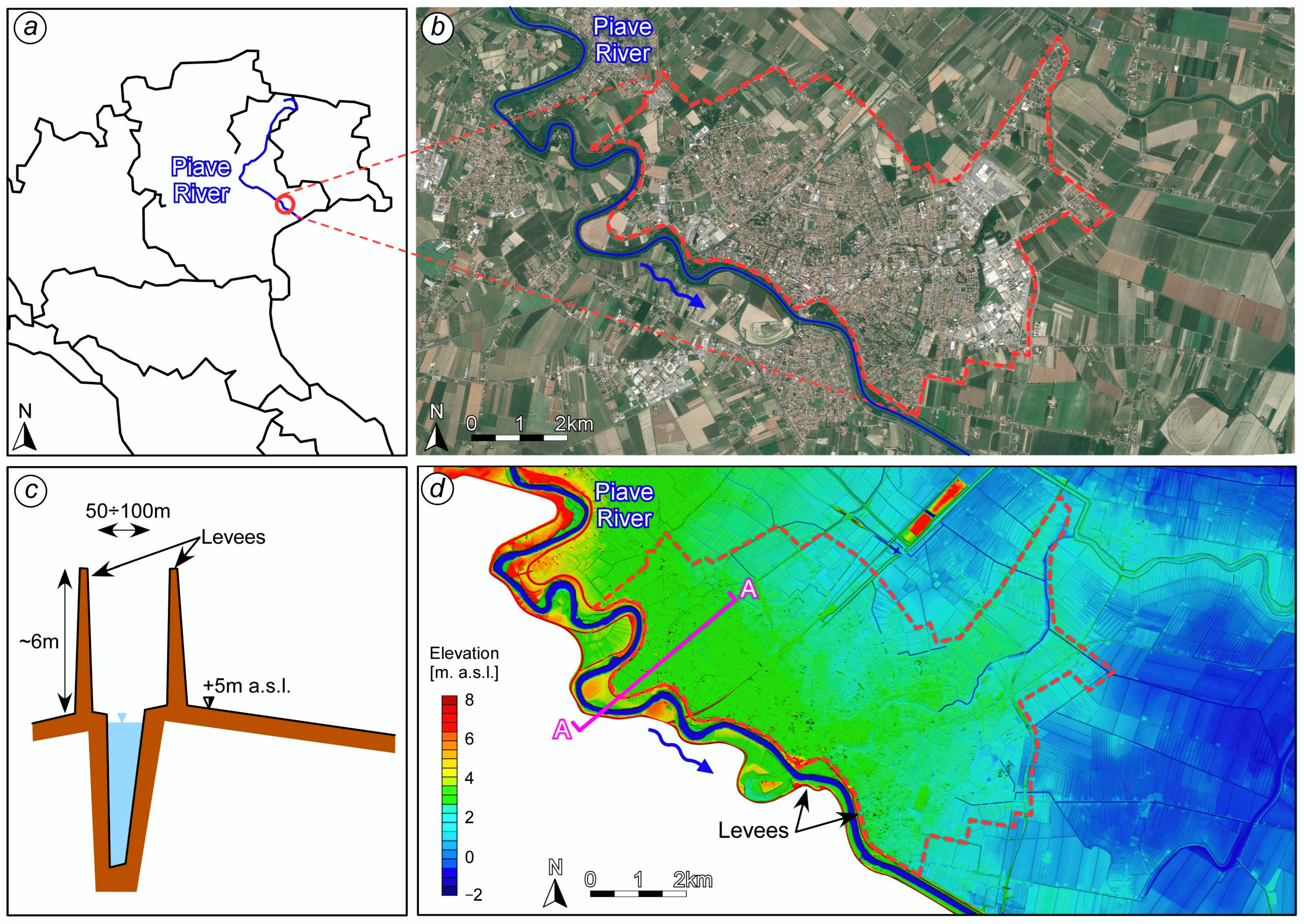
2.1. Study Area and Available GIS Data

The study area (15.04 km2) is located in the northern part of Italy, in the municipality of San Donà di Piave, adjacent to the Piave River (Figure 1a,b). The Piave River is 230 km long; the average flow discharge is of the order of 100 m³/s. Close to the study area, the river has a width spanning from 50 m to 100 m and can convey a discharge as high as ~2700 m³/s during floods. Continuous levees, ~6 m high over the external terrain, separate the compound cross-section of the river from the external floodplains (Figure 1c,d). In the study area, the terrain slope is directed to the south–east, with elevations ranging from 5 m above the sea level (a.s.l.) close to the Piave levees in the northern part to −1 m a.s.l. in the southeastern portion (Figure 1d).
The terrain elevations are derived from LiDAR surveys carried out between 2004 and 2009 by the Italian Ministry of the Environment (http://www.pcn.minambiente.it, accessed on 13 March 2023). Both the digital surface model (DSM) and the digital terrain model (DTM) are available with a spatial resolution of ~1 m. The DSM is derived from the first-pulse data and allows identifying the presence (and the elevation) of treetops and building roofs; in the DTM, data referring to roof and canopy are treated as outlier, and the elevation is interpolated based on that of the neighboring points so as to recover the elevation of the bare soil.
A set of aerial images, taken in 1983, 1990, 1999, and 2004, were extracted from the repository of the Veneto region (https://idt2.regione.veneto.it, accessed on 13 March 2023); additional aerial images, for 2015 and 2021, were retrieved from Google Earth. Technical maps in vector form, derived from photogrammetric data retrieved between 1987 and 2003, were downloaded from the same repository.

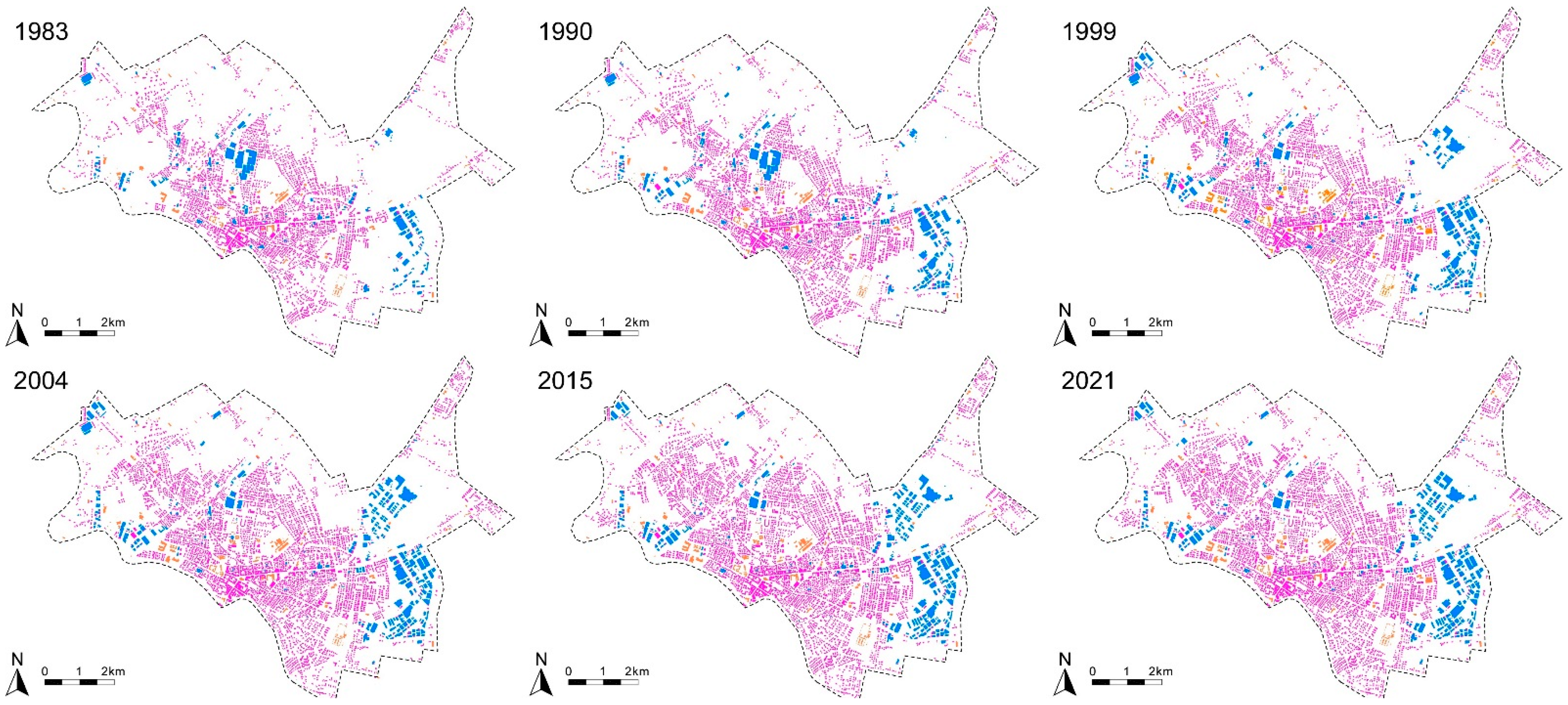
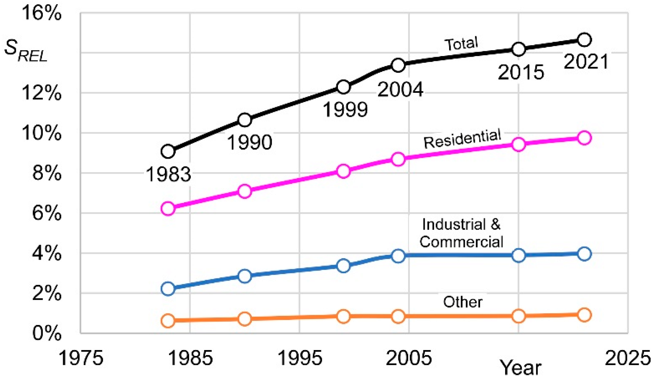
2.2. Tracking the Landscape Change in Time

Exposure to flooding is one of the key parameters in flood risk. Among different possible definitions of exposure [73], here, we consider flood exposure as the presence of items potentially subject to flood damage, which can be quantified through the number or the value of assets in the flood-prone area [49,74]. Changes in time of exposed items and, in particular, residential buildings, are then considered as a proxy for flood risk in the study area.
The evolution of the landscape in the study area was analyzed using the available aerial images. To obtain a digital representation in a vector form of the building footprints at the different years, we started from the building footprints that were present in the technical map, and removed or added building footprints so as to match the configuration of each single aerial image. The six different layouts obtained from the available aerial images are shown in Figure 2, in which the building footprints are grouped into the three categories of residential buildings, industrial and commercial buildings, and other buildings.
Table 1 collects the value of absolute (S) and relative (SREL) footprint surface area, as well as their increase compared to the 1983 initial layout, for the different categories. Areas occupied by residential, industrial/commercial, and other kind of buildings have all increased along the years (see also Figure 3). The largest variation involves the surface occupied by residential buildings, which passes from 937,000 m2 to 1,467,209 m2 (+56.6% in 38 years). In the same period, the areas occupied by industrial/commercial and by other buildings also show large increments, since they have grown by 78.4% and 47.4%, respectively, compared with that of 1983. Globally, considering the whole urban settlement, the footprint area of buildings increased by a factor of 1.61 (from 1.37 km2 to 2.20 km2). A similar trend has been obtained for similar periods in different geographical contexts: de Moel et al. [52] reported factors of 1.94 and 1.50 for the Netherlands in the 1960–2000 and 1980–2015 time intervals, respectively; Jongman et al. [67], for the number of properties in areas at risk and not at risk in the Netherlands, obtained 2.13 and 1.50 for the 1974–2012 time interval; and Fuchs et al. [70] obtained 1.7 for the territory of Austria for the 1977–2015 time interval.
Of course, such an increase in urbanized area has notable implications on flood risk, especially because the region is adjacent to a large river with high levees and insufficient discharge capacity. The Piave River caused various and severe flooding events in the recent past; the most notable example is the disruptive inundation occurred in 1966, when an exceptional flood wave led to the collapse of levees in different parts of the final reach of the Piave River. The return period between of the 1966 flood event at Nervesa della Battaglia (about 40 km upstream of San Donà di Piave) was estimated to be in the range between 100 and 300 years.
The spatial distribution of exposed buildings during the last 40 years, shown in the above Figure 2, allows for some additional considerations. In the 1983 layout, most of the urban settlements were confined in the older, historical center of San Donà di Piave, located in the southwestern part. The industrial and commercial buildings were few and surrounded by relatively large non-built areas; just outside the historical center, the land was mostly agricultural with the presence of a few isolated housing units. In the last few years, the residential areas increased their size along some preferential pathways that changed within the considered period. In 2021, the densely urbanized area has expanded to occupy most of the study area, strongly reducing agricultural land. A similar trend is observed for the industrial and commercial areas. The nature of change in land use is twofold for both the residential and industrial/commercials areas [75,76], consisting of both expansion (i.e., the enlargement of the urban area) and densification (i.e., the increase in building concentration). While the total number of items exposed to a potential flood is greatly increased, not all parts of the study area showed the same developing trend. While the central, residential part has changed little during the years, most of the urbanization involved the surrounding area, where the exposed items increased at a very large rate.
A final important aspect concerns local changes of the topography. In particular, it has to be stressed that the flooding of nearly plain areas is largely affected by the presence of “linear” obstacles, such as road and railway embankments, as well as by the levees of artificial channels forming complex irrigation and drainage networks. In the study area, the DTM includes all the relevant linear obstacle that are present in the most recent layout (i.e., year 2021). To obtain a realistic DTM for the previous scenarios (i.e., 1983 to 2015), the elevation of levees and embankments has been adjusted to match the aerial images.

2.3. Hydrodynamic Model for Hazard Assessment

The hazard scenario is derived using the two-dimensional (2-D) hydrodynamic model 2DEF [44,77,78,79,80,81], which allows for a physics-based description of the flood routing within the Piave River, of the formation of levee failures, and of the flooding of adjacent areas in a coupled fashion. The numerical approach, the model effectiveness in reproducing the river flow, the levee failure, and the subsequent flooding processes have been described in Viero et al. [80]. Essentially, the model solves a modified version of the traditional shallow water equations (SWEs) to account for wetting–drying processes [44,78,79,82], which read:
η ( h ) h t + · q = 0
g h + D D t q Y + J · R e = 0
where t denotes time; (x; y) are the axes of the Cartesian reference frame; g is gravity; h is the free surface elevation; q = (qx; qy) is the depth-integrated velocity (i.e., flow rate per unit width); D/Dt is the Lagrangian (or material) total derivative that lumps local and advective accelerations; Y is the equivalent water depth (i.e., water volume per unit area, see Defina’s [78]); J = (jx, jy) is the energy dissipation due to the bottom stress, which is computed with the Gauckler–Strickler formula; and the tensor Re accounts for the Reynolds stresses in the horizontal plane. In the continuity Equation (1), η(h) is a storativity coefficient that accounts for the wetted areal fraction of the computational domain (it is computed on a cell-by-cell basis, [44,77]).
A mixed Eulerian–Lagrangian approach is used to express the Lagrangian derivative of velocity in the momentum Equation (2) in a finite-difference form [79]. The shallow water equations are then solved using an efficient, semi-implicit, finite element Galerkin method on unstructured triangular grids. As for the modeling of flood-prone rural areas, the model allows coupling 2D triangular cells with one-dimensional (1-D) channel elements to include the main drainage network in a convenient and numerically efficient way. The presence of minor channel networks, such as ditches and furrows, can be accounted for by means of a sub-grid approach for anisotropic flow resistance [83]. Other kinds of 1D special elements [84] allows modeling weirs, sills, regulation devices, pumping stations, and the formation of breaches in earthen levees, induced either by overflowing or by piping [80]. Urbanized areas can be modeled at a large scale by exploiting the efficient artificial porosity approach [77,85].
The model has long been used to study the hydro- and morpho-dynamics of major Italian rivers [32,80,86], as well as lagoon hydro- and morpho-dynamics [87,88], water renewal [89], and temperature dynamics [90] in tidal environments.
In the present study, the computational mesh covers an area of ~589 km2. It includes the Piave River from Nervesa della Battaglia to the mouth in the Adriatic Sea at Cortellazzo, east of the Venice Lagoon. The flexible unstructured grid allows using computational elements of very different sizes, with cell-side length of ~500 m far from the study area, to far less than 10 m in the urban area, where a detailed description is needed. To obtain a detailed description of the flow field in the vicinity of buildings, the building-block technique is used [91]; the polygons describing the building footprint are used to force the generation of the grid, and then the cells that fall within these building footprints are assigned based on the DSM. Then, the elevation of the remaining cells has been assigned based on the DTM, so that the bare soil elevation is considered elsewhere.
The hydrodynamic model of the downstream stretch of the Piave River was calibrated in previous studies [92,93]. Standard values of the Strickler coefficients were given to the computational elements of the external flood-prone areas, depending on the local land-use, and a sensitivity analysis showed that they have a minor impact on the model results. This is because the terrain slope, and in turn the flow velocity, are quite modest in the external area, and the flood pattern is mainly dictated by the embankments and similar obstacles that characterize the local topography.
To generate a verisimilar flood scenario in the study area, we used the flood wave of the recent flood event which occurred in 2018, with a peak discharge of ~2400 m³/s at San Donà di Piave (about 3200 m³/s at Nervesa della Battaglia, corresponding to a return period of about 40 years). While no overflowing nor levee failure were recorded during this event, in the present analysis, we consider a possible levee breach to occur in the upstream part of the analyzed area. The physics-based approach proposed by Viero et al. [80] is used to model the formation and the evolution of the breach in the left levee of the Piave River. A 1D special element at the failure location is used to simulate the initial piping phase, with the progressive erosion of a preferential flow pathway through the core of the levee, up to the collapse of the levee; the breach formation continues by simulating the lateral erosion of the levee margins. During the receding phase of the flood, the shear stresses decrease, thus preventing a further breach enlargement. During the process of breach formation, the discharge through the breach is computed according to the water levels just within and outside the breach, thereby capturing the coupled nature of the phenomenon and the mutual feedbacks of within- and outside-river hydrodynamic processes. For further details, the reader is referred to Viero et al. [80].
In the external areas, the computational domain extends sufficiently so that floodwaters continue flowing toward the downstream low-lying areas, without the need of prescribing outflow boundary conditions close to the study area.

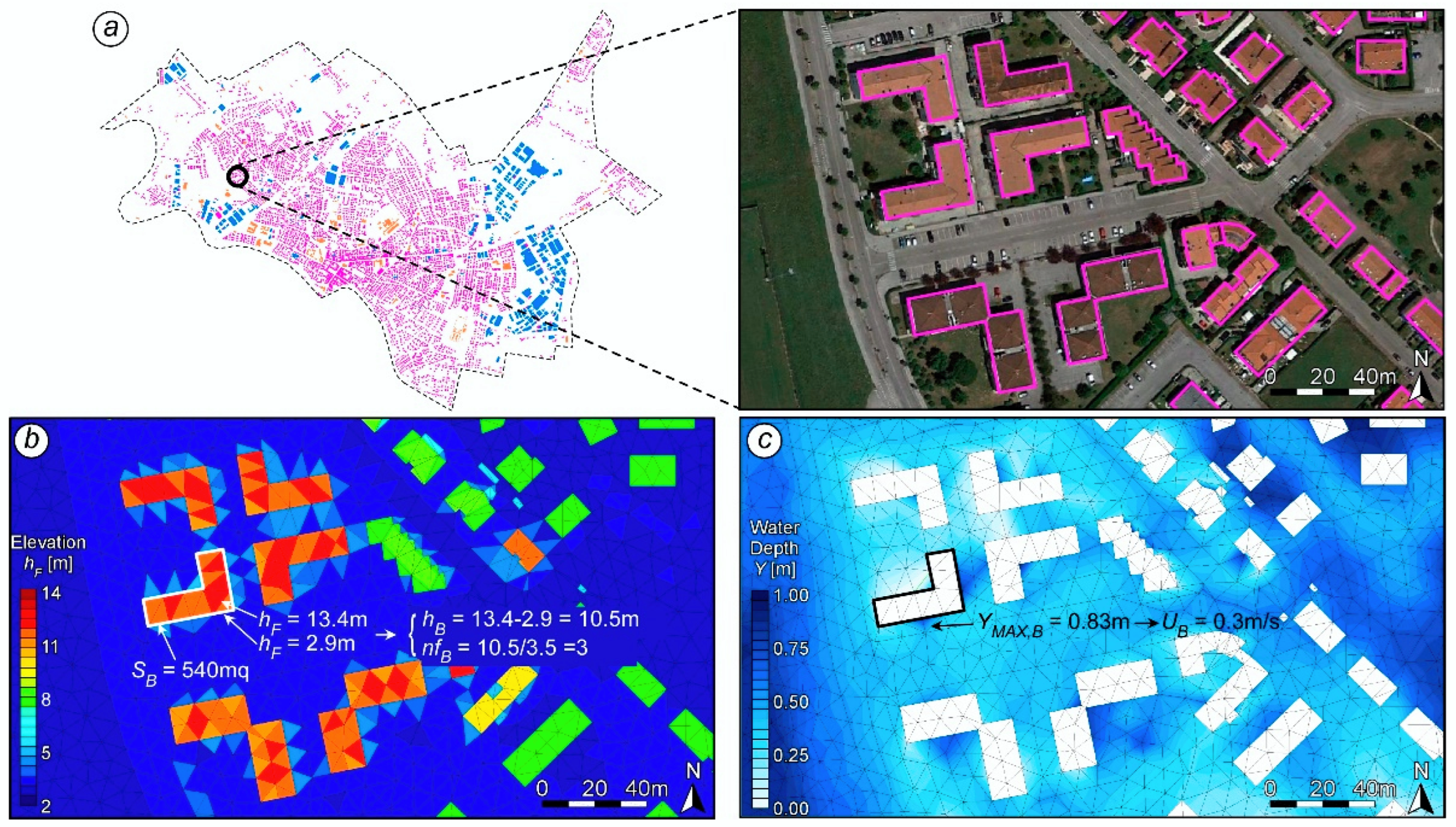
2.4. A Model for the Within-Event Time-Evolution of Damage to Residential Buildings

A damage model has been coupled to the hydrodynamic model 2DEF. In the present analysis, the focus is on the damage pertaining to the residential buildings, and the formulation proposed by Lazzarin et al. [72] has been used for the damage assessment. The parameter W [94] describes the hydrodynamic forcing considering both water depth and velocity from a physical point-of-view; it is defined as a function of the water depth Y and the Froude number F as:
W = Y Y W α 1 + β F 2
with YW = 3.5 m, α = 1.0, and β = 0.3 for residential buildings.
To describe the temporal evolution of the damaging process, the relative damage DREL is computed for each item by integrating over time the rate at which it progresses. The rate is computed using the logistic-type equation:
d D R E L d t = c D R E L 1 γ 1 D R E L m a x V , D R E L 1 + γ
where c is the damage rate factor, γ is a calibration parameter in the range 0 < γ < 1, and V is the vulnerability (i.e., fraction of the exposed items that can be damaged when solicited by a constant hydrodynamic forcing, W, lasting for a reasonably long period of time).
The parameter γ and the functions V(W) and c(W) must be calibrated in a preliminary phase. For residential buildings, through a comparison with the results provided by the synthetic damage model INSYDE [95], Lazzarin et al. [72] found γ = 1.0 and c(W) = pWq (with p = 0.04 h−1, q = 1.3). The vulnerability function is applied in the form V(W) = bWa with a = 0.8 and b = 0.41 for 1-floor buildings, and b equals to 0.22, 0.14, and 0.10 for 2-, 3-, and 4-floor buildings, respectively; when the number of floors, nfB, exceeds 4, b = 0.41/nfB is assumed. In this way, if the water depth is high enough to almost completely damage the ground floor of a building, and not to affect the higher stories, D R E L is close to unity for single-story buildings, and ~1/nfB for multistory buildings.

2.5. Coupling of Hydrodynamic and Damage Models

As damage typically increases with exposure, the different layouts of the study area are expected to produce increasing flood damage through the years [60]. However, different layouts can also change the flood hydrodynamics, which can be affected by the presence or absence of buildings and infrastructures in the urban and peri-urban areas; hence, the hydrodynamic and the damage models have to be run sequentially for each of the six urban layouts considered in the study.
The hydrodynamic model provides water depths and flow velocity at each point of the computational domain for the entire duration of the flood, which are the primary variables for the computation of flood damage to buildings.
To compute the damage, the location and extent of the buildings within the study area are saved as a set of polygons (Figure 4a). For each polygon, which represents a single building (Figure 4b), the model computes the surface area, SB, and identifies the grid cells falling within the polygon and the external cells adjacent to the polygon sides. The height of the building, hB, is estimated as the difference between the elevation, hF, of the cells within the polygon and that of the elements just outside the building footprint. Then, the number of floors, nfB, is determined as a function of the mean inter-floor height (~3 m).
For each time step of the hydrodynamic model and for each polygon, the model evaluates the maximum water depth occurring on the adjacent cells, YMAX,B (Figure 4c). The flow velocity, UB, is then computed by the model at the same cell where the maximum depth occurs. The time-varying hazard degree for each building is estimated in terms of the W parameter, for each item category, according to Equation (3). Given the vulnerability and the damage rate functions, V(W) and c(W), defined for each item category, the model evaluates the within-event time-evolution of the relative damage, DREL, for each object. The monetary damage, D€,REL, can be finally obtained by multiplying DREL by the reconstruction/replacement cost per unit area.
As a simplifying assumption, in the present application to residential buildings, the reconstruction/replacement cost is assumed to be 80% of the market value of the building, where the market value of a residential building in the analyzed area is approximatively composed of the cost of construction (80%) and the value of the land (20%). The market value for the town of San Donà di Piave is found in the database provided by the Italian Revenue Agency (Agenzia delle Entrate). For residential buildings with a normal state of maintenance, values for 2021 range from 1100 EUR /m2 to 1350 EUR /m2. Accordingly, the mean market value is assumed to be 1250 EUR /m2, and the reconstruction/replacement value 1000 EUR /m2. The direct tangible damage D for each building can be estimated as the product of the monetary relative damage D€,REL (per unit area) and the exposed area, which is computed as the product of the footprint surface, SB, and the number of floors, nfB. The total damage D€,TOT affecting the whole region can be finally obtained by adding the values of the damage D for items of all the considered categories. The monetary estimates of damage, associated to previous building layouts, all refer to the present market value; this is equivalent to estimating the expected damage in the present day, supposing that the building layout has not changed since, e.g., 1983. This allows estimating the variation in expected damage ascribed only to landscape change, disregarding the change in time of building value.
In the present study, we only consider the predominant item category, which is that of residential buildings. In general, the model allows the evaluation of damage to different building types using the same procedure (e.g., residential, industrial/commercial, shack). Proper parameters for Equations (3) and (4) have to be specified, of course. Moreover, the damage model can be extended to consider different items (e.g., green areas, agricultural lands, roads); in this case, the description of the hydrodynamic forcing is even easier since the item elevation broadly coincides with the ground elevation, and hence water depth and velocity can be taken directly from the values computed by the model at the given location. Additional important categories exposed to floods include people and vehicles. The model parameter for these categories are already assessed [72,94], but it must be stressed that early warning systems for floods and the proper actions of civil protection can succeed in evacuating people and vehicles with sufficient lead times [96]. Hence, for people and vehicles, the estimation of the real exposure is a challenging task.

3. Results

As anticipated in Section 2.3, flood damage depends on both the exposure (i.e., the layout of buildings and obstacles) and hazard (hydrodynamic flow field as it varies in space and time); the building layout and the hydraulically relevant landscape features also affect the flooding process. Given that the goal of the present study is to highlight the effect of urbanization and landscape modifications on flood damage, as well as to show the potentiality of the damage model recently proposed by Lazzarin et al. [72], we consider a flooding event characterized by the same upstream boundary conditions for all the six layouts (i.e., 1983, 1990, 1999, 2004, 2015, and 2021); that is, the same flood wave is routed within the Piave River and the same levee failure is supposed to occur in all the six different scenarios. Of course, the flood patterns and the local flow field are expected to change in the different layouts because of the landscape modifications.
Evaluating all the components of flood risk as well as computing the real flood risk in rigorous probabilistic framework is beyond the scope of the present work. Hence, we use the expected damage to residential buildings (i.e., the predominant kind of exposed items) as a proxy to track the change in time of flood risk.
In the hypothetical hazard scenario here considered, a levee breach is supposed to form in the left levee of the Piave River due to the onset of a piping erosion process. The discharge through the breach increases fast, up to 500 m³/s at the same time of the flood peak within the Piave River (Figure 5a). The outflow through the breach, which exceeds 20% of the river discharge, produces a significant drawdown within the river (Figure 5b). The water depth in the floodplain just outside of the breach rises up to ~3 m.
Figure 6 shows the evolution in time of the flooded area during the flooding event, computed with the hydrodynamic model for the 1983 and the 2021 layouts of the study area. In both cases, shortly after the levee breaching, water moves eastward. High velocities are observed near the breach location, especially during the first phase of the flooding, and water depths remain quite low. With the flood evolving, floodwaters move to the northeastern part, following the topographic gradient; then, especially in the more recent layouts, a larger portion of water is conveyed southward. About 30 h after the failure, high water depths are observed in the northeastern part of the study area, where the ground elevation is relatively low and the levee of a secondary channel (pink line in Figure 7) acts as an important blocking feature, obstructing the southward waterflow. In the most recent layouts (i.e., 2004, 2015, and 2021) this levee is discontinuous, as an inverted siphon was built to allow for a new road passage. This preferential pathway increases the southward flow rate, reducing the maximum water depths in the northern part of the domain and worsening the hazard scenario in the southern region. Increased flow velocities are found downstream of the levee interruption. In all situations, water is finally conveyed to the southeastern part due to the topographical gradient. The southwestern part of the urban settlements, which coincides with the historical center of San Donà di Piave, is negligibly affected by the flooding event. This is due in part to the location chosen for the levee failure, and in part to the local topography; the ground elevations of the dry region are, on average, 1.5 m higher than the surrounding terrain.
Figure 7 shows the results provided by the hydrodynamic models in terms of maximum water depth, Y, and flow velocity, U, occurred in the course of the flooding events considering the 1983 and the 2021 layouts of the study area.
The coupling of hydrodynamic and damage model, according to the approach proposed by Lazzarin et al. [72], allows for accounting the time evolution of the hazard scenario during a single flooding event, and to estimate the spatially distributed, within-event time evolution of the damage. This is shown in Figure 8, where the relative damage to residential buildings, nfBDREL, is plotted at different time instants for the 1983 and the 2021 layouts (note that the relative damage, DREL, is multiplied by the number of floors, nfB, for normalization purposes, as nfBDREL almost coincides with the damage occurred to the ground floor of multistory buildings). The first aspect to note is the delay in the damage formation with respect to the flooding, which can be appreciated by comparing Figure 6 and Figure 8. Then, the propagation of the flood has a direct influence on the spatial and temporal evolution of the damage (Figure 8). About one day after the beginning of the levee breaching (t = 40 h), only the buildings close to the failure location are damaged. At 50 h, the damage is far greater in the 2021 layout than in 1983, because of the significant urbanization at the northwestern area. At 60 h, in the layout of 1983, the most damaged buildings are those located in the northern part, whereas in 2021, the damage is visibly growing fast, along with the damage in the central and eastern parts of the study area. This is due to the presence of a continuous channel levee in 1983 (highlighted in pink in the above Figure 7), interrupted since the early 2000s for the construction of a new road. The presence of this southward passage causes, in the recent layouts, smaller damages in the northern part, and damaged buildings in the far eastern part. At 70 h, these eastern buildings are also reached and affected by the floods in the 1983 layout, but the damage results are lower than in the 2021 layout.
Numerical values related to effective exposed buildings and to the associated expected damage are reported in Table 2. Passing from the 1983 to the 2021 layout, the total damage, D€,TOT, associated to the considered flooding event shows a considerable increase (+85.5%, Table 2), which is far larger than the increase in both the number of buildings (+43%) and of total building area (+53%). Table 2 shows that not only the exposed buildings have increased in the years, but also the relative damage, DREL,TOT (+21%), leading to a far greater total damage, D€,TOT. This means that the number of exposed buildings has increased much in areas that, in the considered flooding scenario, are relatively hazardous. A second reason that can concur to the increase in relative damage is the different flood propagation due to the presence of a larger number of buildings. In urban areas, the presence of buildings reduces the space for water storage and subsequently increase the water velocity due to narrow paths [77,97]. This is expected to increase both water level and velocity, and hence the expected damage. As an example, Figure 6 shows how the presence of dense buildings in recent layouts modify the propagation of the flood, especially during the first stage of flooding.
Figure 9 shows the within-event time evolution of the total and the relative damage for the different layouts. In particular, Figure 9a shows that, in the time interval between 50 and 70 h, the growing trend of the total damage, D€,TOT (Figure 9a), changes when passing from the 1999 to the 2004 layouts. The relative damage (Figure 9b,c) shows a similar change of trend and, in addition, its value at the end of the flooding event is not monotonically increasing as the significant urban sprawl would suggest. According to Table 2, DREL,TOT passes from 0.0198 to 0.0188 from 1999 to 2004, respectively, and then rises again. This particular occurrence is the outcome of a different flooding process and, in particular, of the construction of the aforementioned new road.

4. Discussion and Conclusions

In this study, flood damage has been analyzed using advanced hydrodynamic and damage models. A study area at a municipality scale, close to the levees of a relatively large river, has been chosen as a representative of the North Italian territory. Here, a large portion of cultivated terrains has been turned into residential areas in the last decades, leading to a massive urbanization of flood-prone areas.
Using available GIS data and aerial images taken at different time instants in the last 40 years, we determined the change of land use at the building scale. The hydrodynamic model solved in a coupled way the propagation of flood within the river, the formation of a hypothetical levee breach by piping erosion, and the ensuing flooding of the external area. The different layouts of buildings, as they changed during the years, were explicitly included in the hydrodynamic model, which allowed for the capture of mutual feedbacks between flooding dynamics and the presence of buildings, i.e., to compute the time-varying hazard conditions for each building in the numerical domain, while accounting for the effects that the presence of buildings exerts on the spreading of floodwaters. Both these aspects are important: the damage depends on the local hazard conditions that can change rapidly in space [62,73,98], and the layout of buildings has also proven to affect the flooding scenario significantly [85,99,100,101,102,103].
The present study confirmed the obvious dependence of flood damage on exposure; in addition, the building-scale analysis showed that exposure is not solely determined by the number (or the value) of buildings exposed to flood. Moreover, given the spatial variability of hazard variables (e.g., water depth and velocity), the location of exposed assets within the flooded areas has shown to play an important part in shaping the potential flood damage. In the present study, while the urbanized area has increased by 53% in the last 40 years, the expected damage has increased by 85%.
The local scale analysis highlighted that the dynamics of the flooding process is of great importance. The space- and time-variations of hazard conditions depend on the propagation of the flood wave in the initially dry land. For nearly flat areas, as is typical for densely populated floodplains, flood propagation is crucially affected by the presence of obstacles and of preferential pathways [13,83,104]. The present study showed that the removal of a short segment of drainage channel levees, substituted with an inverted syphon to construct a new road, produced tangible changes to the flood pattern and, in turn, of the expected damage to buildings. In such kinds of geographical contexts, solving for hydrodynamics using physics-based methods becomes crucial as simplified approaches cannot properly account for the presence of embankments and of relatively small, yet effective, flow pathways [105,106].
The use of an innovative damage model able to track not only the spatial distribution, but also the time evolution of damage in the course of a single flooding event provided additional and useful information. First, the flood duration at each position within the domain is considered naturally and explicitly, allowing us to determine the most critical aspect(s) responsible of the final damage (e.g., maximum flow depth, velocity, or flood duration), and thus to arrange proper defense strategies aimed at reducing the damage. Second, the present model application shows that the within-event time evolution of damage reflected changes in the flooding dynamics.
The study has some limitations. The analysis has been restricted to residential buildings, which provides only a partial view on the multifaceted damage occurring in case of flooding. The choice of using the expected building damage as a proxy for flood risk is partly justified by the fact that residential buildings are by far the principal type of exposed assets. A complete analysis of expected damages should not exclude other categories of assets that are present within the region. For example, as opposed to the increase in damage to buildings, the agricultural loss is expected to decrease due to the reduction in cultivated areas caused by urbanization.
We recapitulate that, in estimating the expected monetary damage, we only considered changes to the building layout, which is recognized as the main factor in damage assessment [107]. The variation in time of the reconstruction/replacement value and of the vulnerability of exposed items have been disregarded. Accordingly, the monetary estimates of damage obtained in this study have the single goal of appreciating the net change in damage ascribed to landscape modifications. Using a constant market value per unit building area while disregarding the role of economical revaluation and the bias of inflation surely allows for clearer comparisons [59].
As a final point, we stress that land-use policies, well-informed from a technical point of view, can substantially contribute to mitigate flood risk, especially in the medium- to the long-term [40,59,108]. While reducing exposure is difficult in already urbanized landscapes, limiting the exposure increase should have a key role in driving land-use policies in developing countries.

Author Contributions

Conceptualization, T.L.; methodology, T.L. and D.P.V.; software, T.L. and D.P.V.; validation, D.P.V. and A.D.; investigation, T.L.; writing—original draft preparation, T.L.; writing—review and editing, D.P.V. and A.D.; visualization, T.L. and D.P.V.; supervision, D.P.V. and A.D. All authors have read and agreed to the published version of the manuscript.

Funding

This research received no external funding.

Data Availability Statement

Aerial photos are taken form Regione Veneto Repository (https://idt2.regione.veneto.it/portfolio/aereofototeca/, accessed on 13 March 2023) and from Google Maps (https://www.google.it/maps/, accessed on 13 March 2023). The regional technical map for Regione Veneto is available at https://idt2.regione.veneto.it/idt/downloader/download (accessed on 13 March 2023).

Conflicts of Interest

The authors declare no conflict of interest.

References

  1. Arnell, N.W.; Gosling, S.N. The Impacts of Climate Change on River Flood Risk at the Global Scale. Clim. Chang. 2016, 134, 387–401. [Google Scholar] [CrossRef] [Green Version]
  2. Cea, L.; Costabile, P. Flood Risk in Urban Areas: Modelling, Management and Adaptation to Climate Change. A Review. Hydrology 2022, 9, 50. [Google Scholar] [CrossRef]
  3. Dottori, F.; Szewczyk, W.; Ciscar, J.-C.; Zhao, F.; Alfieri, L.; Hirabayashi, Y.; Bianchi, A.; Mongelli, I.; Frieler, K.; Betts, R.A.; et al. Increased Human and Economic Losses from River Flooding with Anthropogenic Warming. Nat. Clim. Chang. 2018, 8, 781–786. [Google Scholar] [CrossRef]
  4. Hallegatte, S.; Green, C.; Nicholls, R.J.; Corfee-Morlot, J. Future Flood Losses in Major Coastal Cities. Nat. Clim. Chang. 2013, 3, 802–806. [Google Scholar] [CrossRef]
  5. Hirabayashi, Y.; Mahendran, R.; Koirala, S.; Konoshima, L.; Yamazaki, D.; Watanabe, S.; Kim, H.; Kanae, S. Global Flood Risk under Climate Change. Nat. Clim. Chang. 2013, 3, 816–821. [Google Scholar] [CrossRef]
  6. Kundzewicz, Z.W.; Kanae, S.; Seneviratne, S.I.; Handmer, J.; Nicholls, N.; Peduzzi, P.; Mechler, R.; Bouwer, L.M.; Arnell, N.; Mach, K.; et al. Flood Risk and Climate Change: Global and Regional Perspectives. Hydrol. Sci. J. 2014, 59, 1–28. [Google Scholar] [CrossRef] [Green Version]
  7. Li, C.; Dash, J.; Asamoah, M.; Sheffield, J.; Dzodzomenyo, M.; Gebrechorkos, S.H.; Anghileri, D.; Wright, J. Increased Flooded Area and Exposure in the White Volta River Basin in Western Africa, Identified from Multi-Source Remote Sensing Data. Sci. Rep. 2022, 12, 3701. [Google Scholar] [CrossRef]
  8. Merz, B.; Hall, J.; Disse, M.; Schumann, A. Fluvial Flood Risk Management in a Changing World. Nat. Hazards Earth Syst. Sci. 2010, 10, 509–527. [Google Scholar] [CrossRef] [Green Version]
  9. Meyer, V.; Becker, N.; Markantonis, V.; Schwarze, R.; Van Den Bergh, J.C.J.M.; Bouwer, L.M.; Bubeck, P.; Ciavola, P.; Genovese, E.; Green, C.; et al. Review Article: Assessing the Costs of Natural Hazards-State of the Art and Knowledge Gaps. Nat. Hazards Earth Syst. Sci. 2013, 13, 1351–1373. [Google Scholar] [CrossRef] [Green Version]
  10. Miller, J.D.; Hutchins, M. The Impacts of Urbanisation and Climate Change on Urban Flooding and Urban Water Quality: A Review of the Evidence Concerning the United Kingdom. J. Hydrol. Reg. Stud. 2017, 12, 345–362. [Google Scholar] [CrossRef] [Green Version]
  11. Sampson, C.C.; Smith, A.M.; Bates, P.D.; Neal, J.C.; Alfieri, L.; Freer, J.E. A High-Resolution Global Flood Hazard Model. Water Resour. Res. 2015, 51, 7358–7381. [Google Scholar] [CrossRef] [Green Version]
  12. Sofia, G.; Roder, G.; Dalla Fontana, G.; Tarolli, P. Flood Dynamics in Urbanised Landscapes: 100 Years of Climate and Humans’ Interaction. Sci. Rep. 2017, 7, 40527. [Google Scholar] [CrossRef]
  13. Viero, D.P.; Roder, G.; Matticchio, B.; Defina, A.; Tarolli, P. Floods, Landscape Modifications and Population Dynamics in Anthropogenic Coastal Lowlands: The Polesine (Northern Italy) Case Study. Sci. Total Environ. 2019, 651, 1435–1450. [Google Scholar] [CrossRef]
  14. Winsemius, H.C.; Aerts, J.C.J.H.; van Beek, L.P.H.; Bierkens, M.F.P.; Bouwman, A.; Jongman, B.; Kwadijk, J.C.J.; Ligtvoet, W.; Lucas, P.L.; van Vuuren, D.P.; et al. Global Drivers of Future River Flood Risk. Nat. Clim. Chang. 2016, 6, 381–385. [Google Scholar] [CrossRef] [Green Version]
  15. Doberstein, B.; Fitzgibbons, J.; Mitchell, C. Protect, Accommodate, Retreat or Avoid (PARA): Canadian Community Options for Flood Disaster Risk Reduction and Flood Resilience. Nat. Hazards 2019, 98, 31–50. [Google Scholar] [CrossRef]
  16. Jongman, B. Effective Adaptation to Rising Flood Risk. Nat. Commun. 2018, 9, 1986. [Google Scholar] [CrossRef] [Green Version]
  17. Kundzewicz, Z.W.; Lugeri, N.; Dankers, R.; Hirabayashi, Y.; Döll, P.; Pińskwar, I.; Dysarz, T.; Hochrainer, S.; Matczak, P. Assessing River Flood Risk and Adaptation in Europe—Review of Projections for the Future. Mitig. Adapt. Strateg. Glob. Chang. 2010, 15, 641–656. [Google Scholar] [CrossRef]
  18. Hino, M.; Hall, J. Real Options Analysis of Adaptation to Changing Flood Risk: Structural and Nonstructural Measures. ASCE-ASME J. Risk Uncertain. Eng. Syst. Part Civ. Eng. 2017, 3, 04017005. [Google Scholar] [CrossRef]
  19. Merz, B.; Kreibich, H.; Schwarze, R.; Thieken, A. Assessment of Economic Flood Damage. Nat. Hazards Earth Syst. Sci. 2010, 10, 1697–1724. [Google Scholar] [CrossRef]
  20. Meyer, V.; Priest, S.; Kuhlicke, C. Economic Evaluation of Structural and Non-Structural Flood Risk Management Measures: Examples from the Mulde River. Nat. Hazards 2012, 62, 301–324. [Google Scholar] [CrossRef]
  21. Tariq, M.A.; Farooq, R.; van de Giesen, N. A Critical Review of Flood Risk Management and the Selection of Suitable Measures. Appl. Sci. 2020, 10, 8752. [Google Scholar] [CrossRef]
  22. Di Baldassarre, G.; Castellarin, A.; Brath, A. Analysis of the Effects of Levee Heightening on Flood Propagation: Example of the River Po, Italy. Hydrol. Sci. J. 2009, 54, 1007–1017. [Google Scholar] [CrossRef]
  23. Ludy, J.; Kondolf, G.M. Flood Risk Perception in Lands “Protected” by 100-Year Levees. Nat. Hazards 2012, 61, 829–842. [Google Scholar] [CrossRef]
  24. Collenteur, R.A.; de Moel, H.; Jongman, B.; Di Baldassarre, G. The Failed-Levee Effect: Do Societies Learn from Flood Disasters? Nat. Hazards 2015, 76, 373–388. [Google Scholar] [CrossRef]
  25. Knox, R.L.; Wohl, E.E.; Morrison, R.R. Levees Don’t Protect, They Disconnect: A Critical Review of How Artificial Levees Impact Floodplain Functions. Sci. Total Environ. 2022, 837, 155773. [Google Scholar] [CrossRef]
  26. Hutton, N.S.; Tobin, G.A.; Montz, B.E. The Levee Effect Revisited: Processes and Policies Enabling Development in Yuba County, California. J. Flood Risk Manag. 2019, 12, e12469. [Google Scholar] [CrossRef] [Green Version]
  27. Ferdous, M.R.; Wesselink, A.; Brandimarte, L.; Di Baldassarre, G.; Rahman, M.M. The Levee Effect along the Jamuna River in Bangladesh. Water Int. 2019, 44, 496–519. [Google Scholar] [CrossRef]
  28. McNamara, D.E.; Werner, B.T. Coupled Barrier Island–Resort Model: 1. Emergent Instabilities Induced by Strong Human-Landscape Interactions. J. Geophys. Res. Earth Surf. 2008, 113, F01016. [Google Scholar] [CrossRef]
  29. Werner, B.T.; McNamara, D.E. Dynamics of Coupled Human-Landscape Systems. Geomorphology 2007, 91, 393–407. [Google Scholar] [CrossRef]
  30. Housh, M. Non-Probabilistic Robust Optimization Approach for Flood Control System Design. Environ. Model. Softw. 2017, 95, 48–60. [Google Scholar] [CrossRef]
  31. Kundzewicz, Z.W.; Takeuchi, K. Flood Protection and Management: Quo Vadimus? Hydrol. Sci. J. 1999, 44, 417–432. [Google Scholar] [CrossRef] [Green Version]
  32. Mel, R.A.; Viero, D.P.; Carniello, L.; D’Alpaos, L. Optimal Floodgate Operation for River Flood Management: The Case Study of Padova (Italy). J. Hydrol. Reg. Stud. 2020, 30, 100702. [Google Scholar] [CrossRef]
  33. Merz, B.; Aerts, J.; Arnbjerg-Nielsen, K.; Baldi, M.; Becker, A.; Bichet, A.; Blöschl, G.; Bouwer, L.M.; Brauer, A.; Cioffi, F.; et al. Floods and Climate: Emerging Perspectives for Flood Risk Assessment and Management. Nat. Hazards Earth Syst. Sci. 2014, 14, 1921–1942. [Google Scholar] [CrossRef] [Green Version]
  34. Ventimiglia, U.; Candela, A.; Aronica, G.T. A Cost Efficiency Analysis of Flood Proofing Measures for Hydraulic Risk Mitigation in an Urbanized Riverine Area. Water 2020, 12, 2395. [Google Scholar] [CrossRef]
  35. Botzen, W.J.W.; Aerts, J.C.J.H.; van den Bergh, J.C.J.M. Individual Preferences for Reducing Flood Risk to near Zero through Elevation. Mitig. Adapt. Strateg. Glob. Chang. 2013, 18, 229–244. [Google Scholar] [CrossRef] [Green Version]
  36. de Moel, H.; van Vliet, M.; Aerts, J.C.J.H. Evaluating the Effect of Flood Damage-Reducing Measures: A Case Study of the Unembanked Area of Rotterdam, the Netherlands. Reg. Environ. Chang. 2014, 14, 895–908. [Google Scholar] [CrossRef]
  37. Rehan, B.M. An Innovative Micro-Scale Approach for Vulnerability and Flood Risk Assessment with the Application to Property-Level Protection Adoptions. Nat. Hazards 2018, 91, 1039–1057. [Google Scholar] [CrossRef] [Green Version]
  38. Moftakhari, H.R.; AghaKouchak, A.; Sanders, B.F.; Allaire, M.; Matthew, R.A. What Is Nuisance Flooding? Defining and Monitoring an Emerging Challenge. Water Resour. Res. 2018, 54, 4218–4227. [Google Scholar] [CrossRef]
  39. Kreibich, H.; Thieken, A.H.; Petrow, T.; Müller, M.; Merz, B. Flood Loss Reduction of Private Households Due to Building Precautionary Measures—Lessons Learned from the Elbe Flood in August 2002. Nat. Hazards Earth Syst. Sci. 2005, 5, 117–126. [Google Scholar] [CrossRef] [Green Version]
  40. Zischg, A.P.; Hofer, P.; Mosimann, M.; Röthlisberger, V.; Ramirez, J.A.; Keiler, M.; Weingartner, R. Flood Risk (d)Evolution: Disentangling Key Drivers of Flood Risk Change with a Retro-Model Experiment. Sci. Total Environ. 2018, 639, 195–207. [Google Scholar] [CrossRef]
  41. Tang, J.; Li, Y.; Cui, S.; Xu, L.; Hu, Y.; Ding, S.; Nitivattananon, V. Analyzing the Spatiotemporal Dynamics of Flood Risk and Its Driving Factors in a Coastal Watershed of Southeastern China. Ecol. Indic. 2021, 121, 107134. [Google Scholar] [CrossRef]
  42. Scheuer, S.; Haase, D.; Volk, M. Integrative Assessment of Climate Change for Fast-Growing Urban Areas: Measurement and Recommendations for Future Research. PLoS ONE 2017, 12, e0189451. [Google Scholar] [CrossRef] [PubMed] [Green Version]
  43. Alexakis, D.D.; Grillakis, M.G.; Koutroulis, A.G.; Agapiou, A.; Themistocleous, K.; Tsanis, I.K.; Michaelides, S.; Pashiardis, S.; Demetriou, C.; Aristeidou, K.; et al. GIS and Remote Sensing Techniques for the Assessment of Land Use Change Impact on Flood Hydrology: The Case Study of Yialias Basin in Cyprus. Nat. Hazards Earth Syst. Sci. 2014, 14, 413–426. [Google Scholar] [CrossRef] [Green Version]
  44. Viero, D.P.; Peruzzo, P.; Carniello, L.; Defina, A. Integrated Mathematical Modeling of Hydrological and Hydrodynamic Response to Rainfall Events in Rural Lowland Catchments. Water Resour. Res. 2014, 50, 5941–5957. [Google Scholar] [CrossRef] [Green Version]
  45. Huong, H.T.L.; Pathirana, A. Urbanization and Climate Change Impacts on Future Urban Flooding in Can Tho City, Vietnam. Hydrol. Earth Syst. Sci. 2013, 17, 379–394. [Google Scholar] [CrossRef] [Green Version]
  46. Feng, B.; Zhang, Y.; Bourke, R. Urbanization Impacts on Flood Risks Based on Urban Growth Data and Coupled Flood Models. Nat. Hazards 2021, 106, 613–627. [Google Scholar] [CrossRef]
  47. Beckers, A.; Dewals, B.; Erpicum, S.; Dujardin, S.; Detrembleur, S.; Teller, J.; Pirotton, M.; Archambeau, P. Contribution of Land Use Changes to Future Flood Damage along the River Meuse in the Walloon Region. Nat. Hazards Earth Syst. Sci. 2013, 13, 2301–2318. [Google Scholar] [CrossRef]
  48. Scheuer, S.; Haase, D.; Haase, A.; Wolff, M.; Wellmann, T. A Glimpse into the Future of Exposure and Vulnerabilities in Cities? Modelling of Residential Location Choice of Urban Population with Random Forest. Nat. Hazards Earth Syst. Sci. 2021, 21, 203–217. [Google Scholar] [CrossRef]
  49. de Moel, H.; Jongman, B.; Kreibich, H.; Merz, B.; Penning-Rowsell, E.; Ward, P.J. Flood Risk Assessments at Different Spatial Scales. Mitig. Adapt. Strateg. Glob. Chang. 2015, 20, 865–890. [Google Scholar] [CrossRef] [Green Version]
  50. Kundzewicz, Z.W.; Pińskwar, I.; Brakenridge, G.R. Large Floods in Europe, 1985–2009. Hydrol. Sci. J. 2013, 58, 1–7. [Google Scholar] [CrossRef]
  51. Barredo, J.I. Normalised Flood Losses in Europe: 1970–2006. Nat. Hazards Earth Syst. Sci. 2009, 9, 97–104. [Google Scholar] [CrossRef]
  52. de Moel, H.; Aerts, J.C.J.H.; Koomen, E. Development of Flood Exposure in the Netherlands during the 20th and 21st Century. Spec. Issue Polit. Policy Carbon Capture Storage 2011, 21, 620–627. [Google Scholar] [CrossRef]
  53. Neumayer, E.; Barthel, F. Normalizing Economic Loss from Natural Disasters: A Global Analysis. Glob. Environ. Chang. 2011, 21, 13–24. [Google Scholar] [CrossRef] [Green Version]
  54. Preston, B.L. Local Path Dependence of U.S. Socioeconomic Exposure to Climate Extremes and the Vulnerability Commitment. Glob. Environ. Chang. 2013, 23, 719–732. [Google Scholar] [CrossRef]
  55. Ceola, S.; Laio, F.; Montanari, A. Satellite Nighttime Lights Reveal Increasing Human Exposure to Floods Worldwide. Geophys. Res. Lett. 2014, 41, 7184–7190. [Google Scholar] [CrossRef]
  56. Ceola, S.; Laio, F.; Montanari, A. Human-Impacted Waters: New Perspectives from Global High-Resolution Monitoring. Water Resour. Res. 2015, 51, 7064–7079. [Google Scholar] [CrossRef]
  57. Mård, J.; Di Baldassarre, G.; Mazzoleni, M. Nighttime Light Data Reveal How Flood Protection Shapes Human Proximity to Rivers. Sci. Adv. 2018, 4, eaar5779. [Google Scholar] [CrossRef] [Green Version]
  58. Berndtsson, R.; Becker, P.; Persson, A.; Aspegren, H.; Haghighatafshar, S.; Jönsson, K.; Larsson, R.; Mobini, S.; Mottaghi, M.; Nilsson, J.; et al. Drivers of Changing Urban Flood Risk: A Framework for Action. J. Environ. Manage 2019, 240, 47–56. [Google Scholar] [CrossRef]
  59. Elmer, F.; Hoymann, J.; Düthmann, D.; Vorogushyn, S.; Kreibich, H. Drivers of Flood Risk Change in Residential Areas. Nat. Hazards Earth Syst. Sci. 2012, 12, 1641–1657. [Google Scholar] [CrossRef] [Green Version]
  60. Domeneghetti, A.; Carisi, F.; Castellarin, A.; Brath, A. Evolution of Flood Risk over Large Areas: Quantitative Assessment for the Po River. J. Hydrol. 2015, 527, 809–823. [Google Scholar] [CrossRef]
  61. Cammerer, H.; Thieken, A.H. Historical Development and Future Outlook of the Flood Damage Potential of Residential Areas in the Alpine Lech Valley (Austria) between 1971 and 2030. Reg. Environ. Chang. 2013, 13, 999–1012. [Google Scholar] [CrossRef]
  62. Löschner, L.; Herrnegger, M.; Apperl, B.; Senoner, T.; Seher, W.; Nachtnebel, H.P. Flood Risk, Climate Change and Settlement Development: A Micro-Scale Assessment of Austrian Municipalities. Reg. Environ. Chang. 2017, 17, 311–322. [Google Scholar] [CrossRef] [Green Version]
  63. Wang, Y.-J.; Gao, C.; Zhai, J.-Q.; Li, X.-C.; Su, B.; Hartmann, H. Spatio-Temporal Changes of Exposure and Vulnerability to Floods in China. Spec. Top. Chinas Carbon Emiss. Peaking 2014, 5, 197–205. [Google Scholar] [CrossRef]
  64. Cammerer, H.; Thieken, A.H.; Verburg, P.H. Spatio-Temporal Dynamics in the Flood Exposure Due to Land Use Changes in the Alpine Lech Valley in Tyrol (Austria). Nat. Hazards 2013, 68, 1243–1270. [Google Scholar] [CrossRef]
  65. Bouwer, L.M. Projections of Future Extreme Weather Losses Under Changes in Climate and Exposure. Risk Anal. 2013, 33, 915–930. [Google Scholar] [CrossRef] [PubMed]
  66. Figueiredo, R.; Martina, M. Using Open Building Data in the Development of Exposure Data Sets for Catastrophe Risk Modelling. Nat. Hazards Earth Syst. Sci. 2016, 16, 417–429. [Google Scholar] [CrossRef] [Green Version]
  67. Jongman, B.; Koks, E.E.; Husby, T.G.; Ward, P.J. Increasing Flood Exposure in the Netherlands: Implications for Risk Financing. Nat. Hazards Earth Syst. Sci. 2014, 14, 1245–1255. [Google Scholar] [CrossRef] [Green Version]
  68. Chen, A.S.; Hammond, M.J.; Djordjević, S.; Butler, D.; Khan, D.M.; Veerbeek, W. From Hazard to Impact: Flood Damage Assessment Tools for Mega Cities. Nat. Hazards 2016, 82, 857–890. [Google Scholar] [CrossRef] [Green Version]
  69. Röthlisberger, V.; Zischg, A.P.; Keiler, M. Identifying Spatial Clusters of Flood Exposure to Support Decision Making in Risk Management. Sci. Total Environ. 2017, 598, 593–603. [Google Scholar] [CrossRef] [Green Version]
  70. Fuchs, S.; Keiler, M.; Zischg, A. A Spatiotemporal Multi-Hazard Exposure Assessment Based on Property Data. Nat. Hazards Earth Syst. Sci. 2015, 15, 2127–2142. [Google Scholar] [CrossRef] [Green Version]
  71. Jongman, B.; Kreibich, H.; Apel, H.; Barredo, J.I.; Bates, P.D.; Feyen, L.; Gericke, A.; Neal, J.; Aerts, J.C.J.H.; Ward, P.J. Comparative Flood Damage Model Assessment: Towards a European Approach. Nat. Hazards Earth Syst. Sci. 2012, 12, 3733–3752. [Google Scholar] [CrossRef] [Green Version]
  72. Lazzarin, T.; Viero, D.P.; Molinari, D.; Ballio, F.; Defina, A. A New Framework for Flood Damage Assessment Considering the Within-Event Time Evolution of Hazard, Exposure, and Vulnerability. J. Hydrol. 2022, 615PA, 128687. [Google Scholar] [CrossRef]
  73. O’Neill, E.; Brereton, F.; Shahumyan, H.; Clinch, J.P. The Impact of Perceived Flood Exposure on Flood-Risk Perception: The Role of Distance. Risk Anal. 2016, 36, 2158–2186. [Google Scholar] [CrossRef] [PubMed]
  74. Ţîncu, R.; Zêzere, J.L.; Lazar, G. Identification of Elements Exposed to Flood Hazard in a Section of Trotus River, Romania. Geomat. Nat. Hazards Risk 2018, 9, 950–969. [Google Scholar] [CrossRef] [Green Version]
  75. Broitman, D.; Koomen, E. Residential Density Change: Densification and Urban Expansion. Comput. Environ. Urban Syst. 2015, 54, 32–46. [Google Scholar] [CrossRef]
  76. Mustafa, A.; Bruwier, M.; Archambeau, P.; Erpicum, S.; Pirotton, M.; Dewals, B.; Teller, J. Effects of Spatial Planning on Future Flood Risks in Urban Environments. J. Environ. Manage 2018, 225, 193–204. [Google Scholar] [CrossRef]
  77. Viero, D.P. Modelling Urban Floods Using a Finite Element Staggered Scheme with an Anisotropic Dual Porosity Model. J. Hydrol. 2019, 568, 247–259. [Google Scholar] [CrossRef] [Green Version]
  78. Defina, A. Two-Dimensional Shallow Flow Equations for Partially Dry Areas. Water Resour. Res. 2000, 36, 3251–3264. [Google Scholar] [CrossRef] [Green Version]
  79. Defina, A. Numerical Experiments on Bar Growth. Water Resour. Res. 2003, 39, 1092. [Google Scholar] [CrossRef]
  80. Viero, D.P.; D’Alpaos, A.; Carniello, L.; Defina, A. Mathematical Modeling of Flooding Due to River Bank Failure. Adv. Water Resour. 2013, 59, 82–94. [Google Scholar] [CrossRef]
  81. Lazzarin, T.; Viero, D.P. Curvature-Induced Secondary Flow in 2D Depth-Averaged Hydro-Morphodynamic Models: An Assessment of Different Approaches and Key Factors. Adv. Water Resour. 2023, 171, 104355. [Google Scholar] [CrossRef]
  82. D’Alpaos, L.; Defina, A. Mathematical Modeling of Tidal Hydrodynamics in Shallow Lagoons: A Review of Open Issues and Applications to the Venice Lagoon. Comput. Geosci. 2007, 33, 476–496. [Google Scholar] [CrossRef]
  83. Viero, D.P.; Valipour, M. Modeling Anisotropy in Free-Surface Overland and Shallow Inundation Flows. Adv. Water Resour. 2017, 104, 1–14. [Google Scholar] [CrossRef]
  84. Martini, P.; Carniello, L.; Avanzi, C. Two Dimensional Modelling of Flood Flows and Suspended Sediment transport: The Case of the Brenta River, Veneto (Italy). Nat. Hazards Earth Syst. Sci. 2004, 4, 165–181. [Google Scholar] [CrossRef] [Green Version]
  85. Ferrari, A.; Viero, D.P. Floodwater Pathways in Urban Areas: A Method to Compute Porosity Fields for Anisotropic Subgrid Models in Differential Form. J. Hydrol. 2020, 589, 125193. [Google Scholar] [CrossRef]
  86. Mel, R.A.; Viero, D.P.; Carniello, L.; D’Alpaos, L. Multipurpose Use of Artificial Channel Networks for Flood Risk Reduction: The Case of the Waterway Padova–Venice (Italy). Water 2020, 12, 1609. [Google Scholar] [CrossRef]
  87. Mel, R.A.; Viero, D.P.; Carniello, L.; Defina, A.; D’Alpaos, L. The First Operations of Mo.S.E. System to Prevent the Flooding of Venice: Insights on the Hydrodynamics of a Regulated Lagoon. Estuar. Coast. Shelf Sci. 2021, 261, 107547. [Google Scholar] [CrossRef]
  88. Tognin, D.; Finotello, A.; D’Alpaos, A.; Viero, D.P.; Pivato, M.; Mel, R.A.; Defina, A.; Bertuzzo, E.; Marani, M.; Carniello, L. Loss of Geomorphic Diversity in Shallow Tidal Embayments Promoted by Storm-Surge Barriers. Sci. Adv. 2022, 8, eabm8446. [Google Scholar] [CrossRef]
  89. Viero, D.P.; Defina, A. Water Age, Exposure Time, and Local Flushing Time in Semi-Enclosed, Tidal Basins with Negligible Freshwater Inflow. J. Mar. Syst. 2016, 156, 16–29. [Google Scholar] [CrossRef]
  90. Pivato, M.; Carniello, L.; Viero, D.P.; Soranzo, C.; Defina, A.; Silvestri, S. Remote Sensing for Optimal Estimation of Water Temperature Dynamics in Shallow Tidal Environments. Remote Sens. 2020, 12, 51. [Google Scholar] [CrossRef] [Green Version]
  91. Schubert, J.E.; Sanders, B.F. Building Treatments for Urban Flood Inundation Models and Implications for Predictive Skill and Modeling Efficiency. Adv. Water Resour. 2012, 41, 49–64. [Google Scholar] [CrossRef]
  92. Crestani, E.; Passadore, G.; Mel, R.A.; Bertuzzo, E.; Viero, D.P.; Carniello, L.; Rinaldo, A.; D’Alpaos, L. Ricostruzione Modellistica della Piena dell’Ottobre 2018 nel Bacino del Fiume Piave. In Proceedings of the XXXVII Italian conference of Hydraulics and Hydraulic Works, Online, 14–16 June 2021. [Google Scholar]
  93. Crestani, E.; Passadore, G.; Viero, D.P.; Carniello, L.; D’Alpaos, L.; Rinaldo, A. Sistema Integrato di Previsione delle Piene in Tempo Reale nel Bacino Idrografico del Piave. In Proceedings of the XXXVIII Italian Conference of Hydraulics and Hydraulic Works, Reggio Calabria, Italy, 4–7 September 2022. [Google Scholar]
  94. Lazzarin, T.; Viero, D.P.; Molinari, D.; Ballio, F.; Defina, A. Flood Damage Functions Based on a Single Physics- and Data-Based Impact Parameter That Jointly Accounts for Water Depth and Velocity. J. Hydrol. 2022, 607, 127485. [Google Scholar] [CrossRef]
  95. Dottori, F.; Figueiredo, R.; Martina, M.L.V.; Molinari, D.; Scorzini, A.R. INSYDE: A Synthetic, Probabilistic Flood Damage Model Based on Explicit Cost Analysis. Nat. Hazards Earth Syst. Sci. 2016, 16, 2577–2591. [Google Scholar] [CrossRef] [Green Version]
  96. Arrighi, C.; Pregnolato, M.; Dawson, R.J.; Castelli, F. Preparedness against Mobility Disruption by Floods. Sci. Total Environ. 2019, 654, 1010–1022. [Google Scholar] [CrossRef] [PubMed]
  97. Ferrari, A.; Viero, D.P.; Vacondio, R.; Defina, A.; Mignosa, P. Flood Inundation Modeling in Urbanized Areas: A Mesh-Independent Porosity Approach with Anisotropic Friction. Adv. Water Resour. 2019, 125, 98–113. [Google Scholar] [CrossRef]
  98. Molinari, D.; Dazzi, S.; Gattai, E.; Minucci, G.; Pesaro, G.; Radice, A.; Vacondio, R. Cost–Benefit Analysis of Flood Mitigation Measures: A Case Study Employing High-Performance Hydraulic and Damage Modelling. Nat. Hazards 2021, 108, 3061–3084. [Google Scholar] [CrossRef]
  99. Li, X.; Erpicum, S.; Mignot, E.; Archambeau, P.; Pirotton, M.; Dewals, B. Influence of Urban Forms on Long-Duration Urban Flooding: Laboratory Experiments and Computational Analysis. J. Hydrol. 2021, 603, 127034. [Google Scholar] [CrossRef]
  100. Wang, Y.; Chen, A.S.; Fu, G.; Djordjević, S.; Zhang, C.; Savić, D.A. An Integrated Framework for High-Resolution Urban Flood Modelling Considering Multiple Information Sources and Urban Features. Environ. Model. Softw. 2018, 107, 85–95. [Google Scholar] [CrossRef]
  101. Mejía-Morales, M.A.; Mignot, E.; Paquier, A.; Sigaud, D.; Proust, S. Impact of the Porosity of an Urban Block on the Flood Risk Assessment: A Laboratory Experiment. J. Hydrol. 2021, 602, 126715. [Google Scholar] [CrossRef]
  102. Meesuk, V.; Vojinovic, Z.; Mynett, A.E.; Abdullah, A.F. Urban Flood Modelling Combining Top-View LiDAR Data with Ground-View SfM Observations. Adv. Water Resour. 2015, 75, 105–117. [Google Scholar] [CrossRef]
  103. Mignot, E.; Paquier, A.; Haider, S. Modeling Floods in a Dense Urban Area Using 2D Shallow Water Equations. J. Hydrol. 2006, 327, 186–199. [Google Scholar] [CrossRef] [Green Version]
  104. Hailemariam, F.M.; Brandimarte, L.; Dottori, F. Investigating the Influence of Minor Hydraulic Structures on Modeling Flood Events in Lowland Areas. Hydrol. Process. 2014, 28, 1742–1755. [Google Scholar] [CrossRef]
  105. Manfreda, S.; Nardi, F.; Samela, C.; Grimaldi, S.; Taramasso, A.C.; Roth, G.; Sole, A. Investigation on the Use of Geomorphic Approaches for the Delineation of Flood Prone Areas. J. Hydrol. 2014, 517, 863–876. [Google Scholar] [CrossRef]
  106. Dottori, F.; Martina, M.L.V.; Figueiredo, R. A Methodology for Flood Susceptibility and Vulnerability Analysis in Complex Flood Scenarios. J. Flood Risk Manag. 2018, 11, S632–S645. [Google Scholar] [CrossRef]
  107. Molinari, D.; Scorzini, A.R. On the Influence of Input Data Quality to Flood Damage Estimation: The Performance of the INSYDE Model. Water Switz. 2017, 9, 688. [Google Scholar] [CrossRef] [Green Version]
  108. Gabriels, K.; Willems, P.; Van Orshoven, J. A Comparative Flood Damage and Risk Impact Assessment of Land Use Changes. Nat. Hazards Earth Syst. Sci. 2022, 22, 395–410. [Google Scholar] [CrossRef]
Figure 1. Study area: (a) location in the north of Italy; (b) aerial view of the study area in the San Donà di Piave Municipality with the course of the Piave River in blue; (c) schematic of cross-section A-A (out of scale); (d) the DTM with elevations in meters above the sea level (a.s.l.).
Geosciences 13 00112 g001
Figure 2. Maps of the building footprints in the study area in the last 40 years: residential buildings (pink), industrial and commercial buildings (blue), and other buildings (orange).
Geosciences 13 00112 g002
Figure 3. Relative footprint surface (SREL) through the years for the different categories of buildings in the study area.
Geosciences 13 00112 g003
Figure 4. Method to compute flood damage. (a) Study area with a zoomed-in view of building footprint superimposed on the aerial image; (b) computational grid with details of the estimation of the surface SB and the number of floors nfB of buildings; (c) plot of instantaneous water depths with details of the estimation of the hydrodynamic forcing on a single building. (i.e., maximum surrounding water depth YMAX,B and velocity UB).
Geosciences 13 00112 g004
Figure 5. Hazard scenario. (a) Discharge hydrographs within the Piave River upstream (solid line) and downstream (dash-dotted line) of the levee breach location and through the breach (dotted line); (b) water levels within the Piave River with (solid line) and without (dashed line) the breach formation, and just outside of the levee breach location (dotted line).
Geosciences 13 00112 g005
Figure 6. Spatial distribution of the water depth, Y, during the flooding event in the 1983 layout (upper panels) and in the 2021 layout (lower panels).
Geosciences 13 00112 g006
Figure 7. Results of the hydrodynamic simulation in terms of maximum water depth (left) and flow velocity (right) as a consequence of the failure of the left levee of the Piave River. The results refer to the 1983 and the 2021 layouts (upper and lower panels, respectively).
Geosciences 13 00112 g007
Figure 8. Spatial distribution of the relative damage to residential buildings referred to the ground floor, nfBDREL, during the flooding event for the layout of 1983 (upper panels) and of 2021 (lower panels). Dots correspond to single buildings.
Geosciences 13 00112 g008
Figure 9. Temporal evolution of (a) the total damage D€,TOT, (b) the relative damage DREL,TOT, and (c) the relative damage referred to the ground floor, for residential buildings for the different layouts since 1983 to 2021.
Geosciences 13 00112 g009
Table 1. Absolute (S) and relative (SREL) footprint surface area and their increase compared to the 1983 layout, for different building categories in the study area during the last 40 years.
ResidentialIndustrial and CommercialOtherTotal
YearS [m2]SREL% *S [m2]SREL% *S [m2]SREL% *S [m2]SREL% *
1983937,0000.0623 334,7870.0223 94,9350.0063 1,366,7220.0909
19901,066,0440.0709+13.8%428,9820.0285+28.1%107,0510.0071+12.8%1,602,0770.1065+17.2%
19991,217,5340.0809+29.9%507,2250.0337+51.5%127,0150.0084+33.8%1,851,7740.1231+35.5%
20041,306,6760.0869+39.5%579,3610.0385+73.1%128,2650.0085+35.1%2,014,3020.1339+47.4%
20151,419,0700.0943+51.4%585,4360.0389+74.9%130,0070.0086+36.9%2,134,5130.1419+56.2%
20211,467,2090.0975+56.6%597,1650.0397+78.4%139,9760.0093+47.4%2,204,3500.1466+61.3%
* Increase since 1983.
Table 2. Characteristics of exposed residential buildings through the years: number of buildings, footprint area S, average number of floors nfB and exposed area SnfB (with its increase compared to 1983). Results of the model for the simulated levee failure considering the different yearly layout: total damage D€,TOT, relative damage DREL,TOT and relative damage for the first floor nfB·DREL,TOT (with the corresponding increase compared to 1983).
Yearn. of
Buildings
Mean nfBSnfB [m2]% *D€,TOT [EUR]% *DREL,TOT% *nfBDREL,TOT% *
198352843.2113,008,767 51,634,419 0.0172 0.0551
199059013.1933,404,31813.1%59,939,23616.1%0.01762.6%0.05622.0%
199966103.1923,886,34829.2%77,139,89349.4%0.019815.7%0.063415.0%
200471423.1734,145,50037.8%77,869,61650.8%0.01889.5%0.05968.1%
201574613.1524,472,64448.7%88,575,56871.5%0.019815.4%0.062413.3%
202175693.1434,610,81953.2%95,775,64685.5%0.020821.0%0.065318.5%
* Increase compared to 1983.
Disclaimer/Publisher’s Note: The statements, opinions and data contained in all publications are solely those of the individual author(s) and contributor(s) and not of MDPI and/or the editor(s). MDPI and/or the editor(s) disclaim responsibility for any injury to people or property resulting from any ideas, methods, instructions or products referred to in the content.

