
Multiscale Characterization of Fracture Patterns: A Case Study of the Noble Hills Range (Death Valley, CA, USA), Application to Geothermal Reservoirs


Abstract
:1. Introduction
- a 2D characterization of the NH fracture network;
- a multiscale evolution of length distributions;
- evaluate the fracture system in the complex tectonic and geometrical setting;
- present a conceptual scheme of the NH fracture network organization, and the role of each fracture order of magnitude on the connectivity.
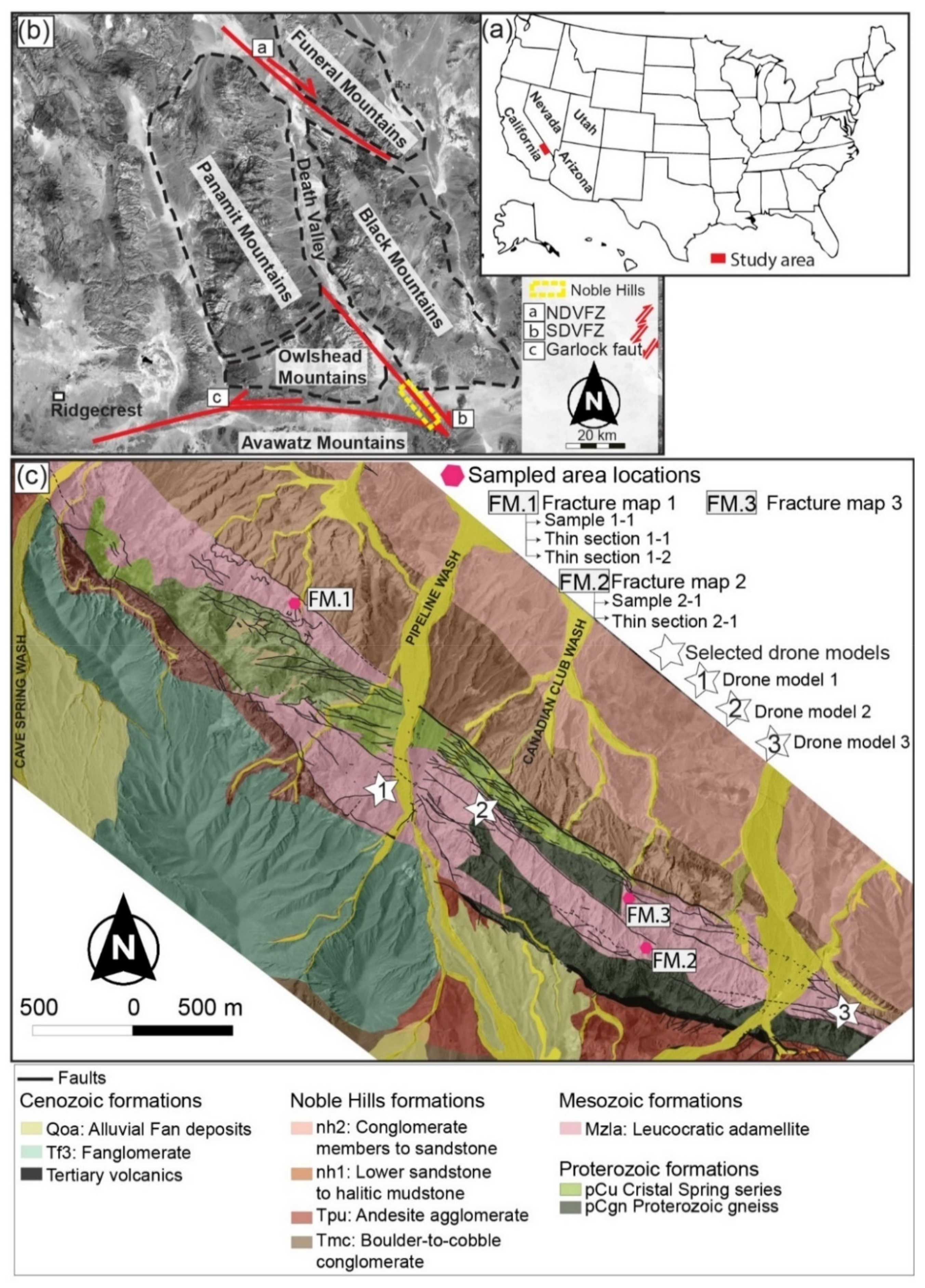
2. Geological Setting
3. Materials and Methods
3.1. Materials
3.1.1. Large Scale Characterization
3.1.2. Photogrammetric Study/Analysis
3.1.3. Fracture Map Characterization
3.2. Methods
3.2.1. Fractures Acquisition
3.2.2. Fractures Analysis
4. Results
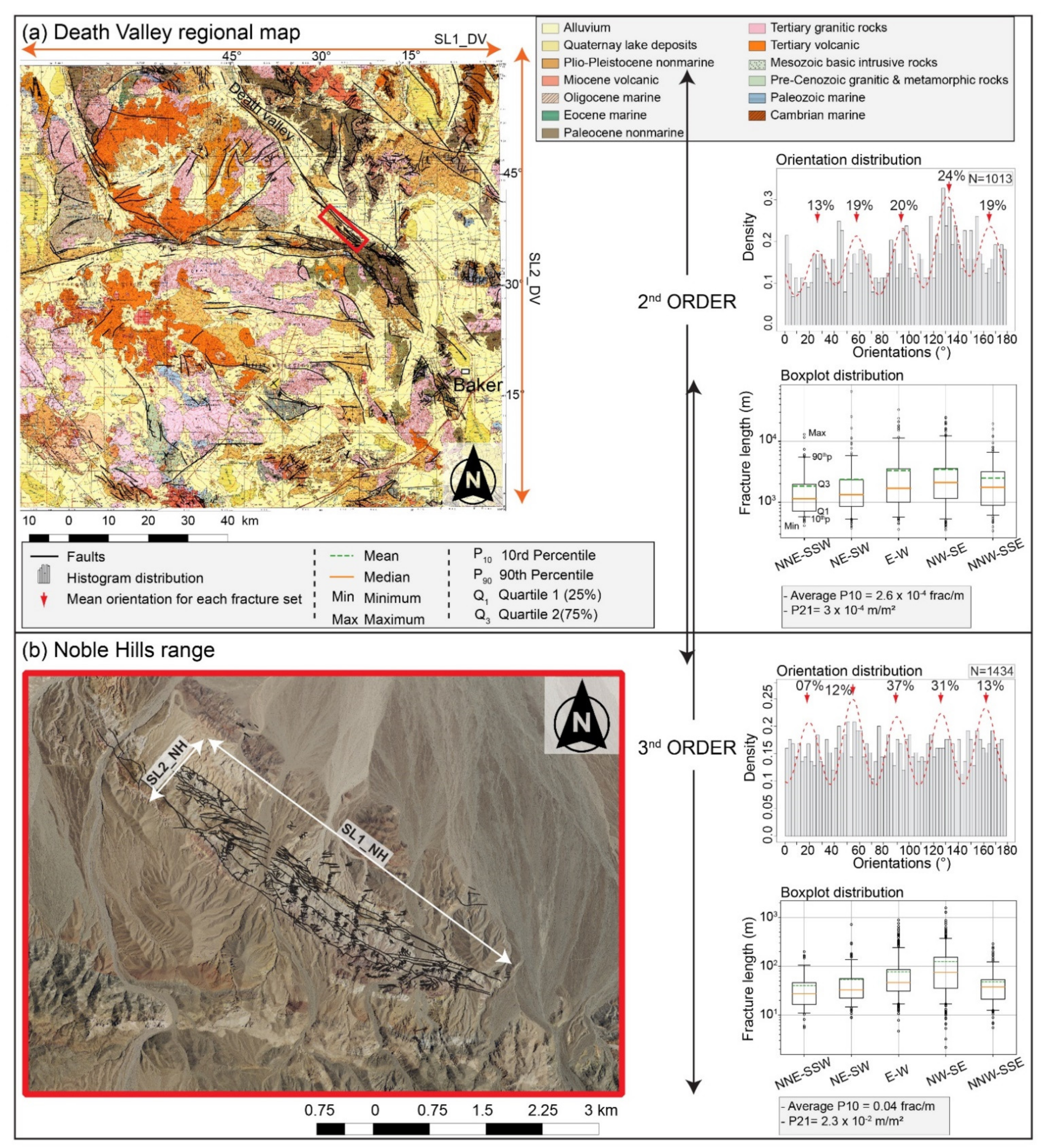
4.1. Large Scale Domains
4.2. Photogrammetric Models
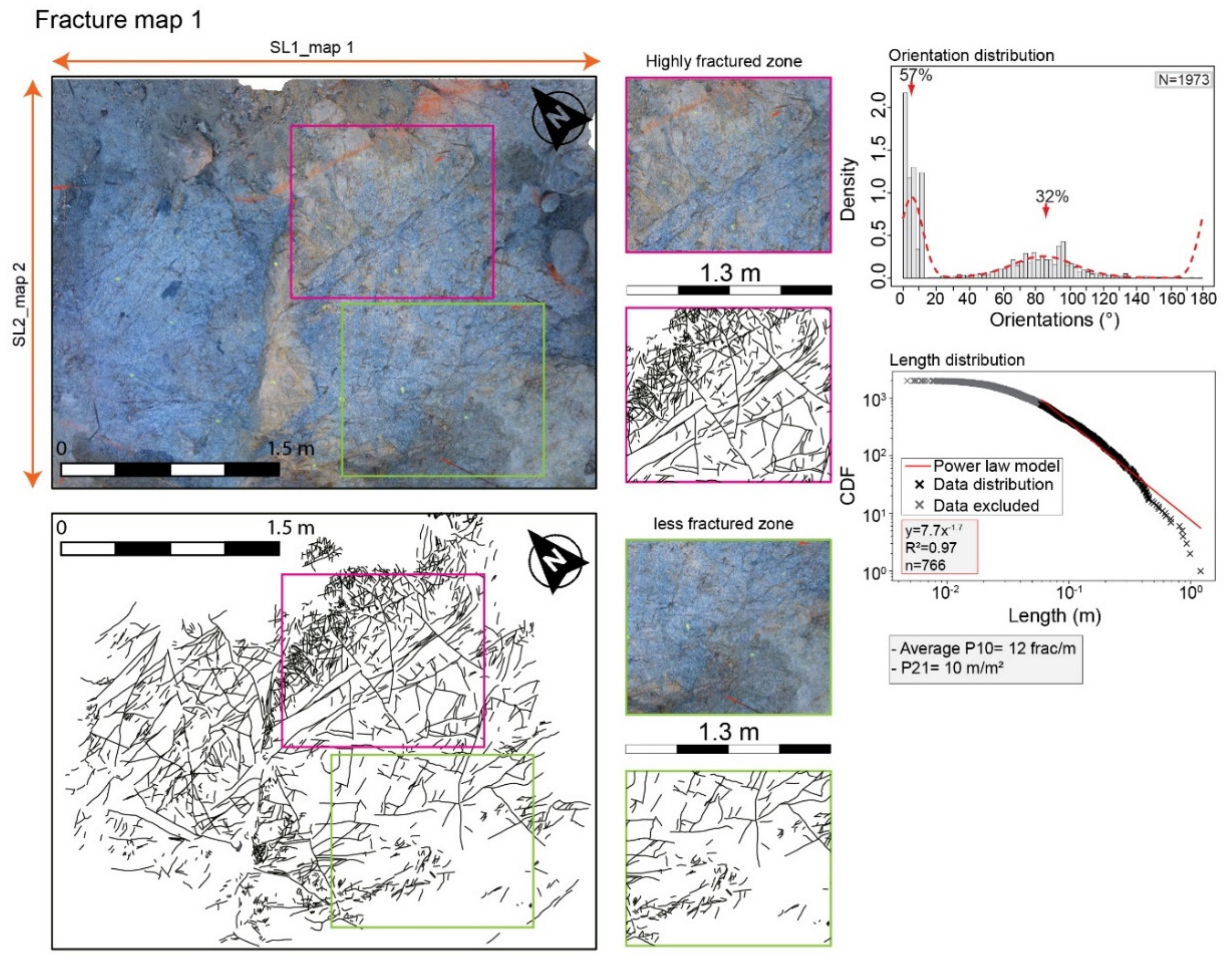
4.3. Fracture Maps
5. Discussion
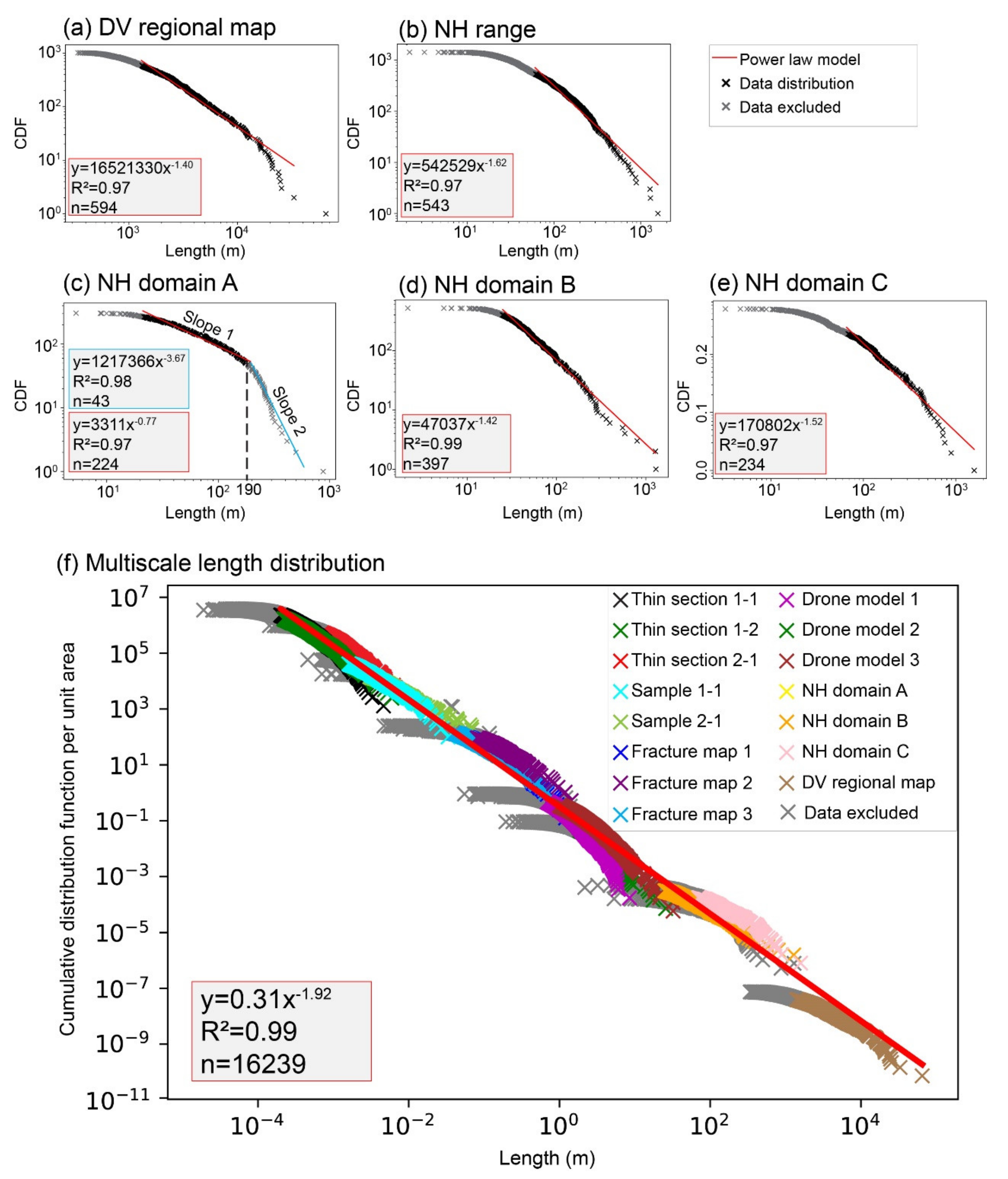
5.1. Multiscale Length Characterization
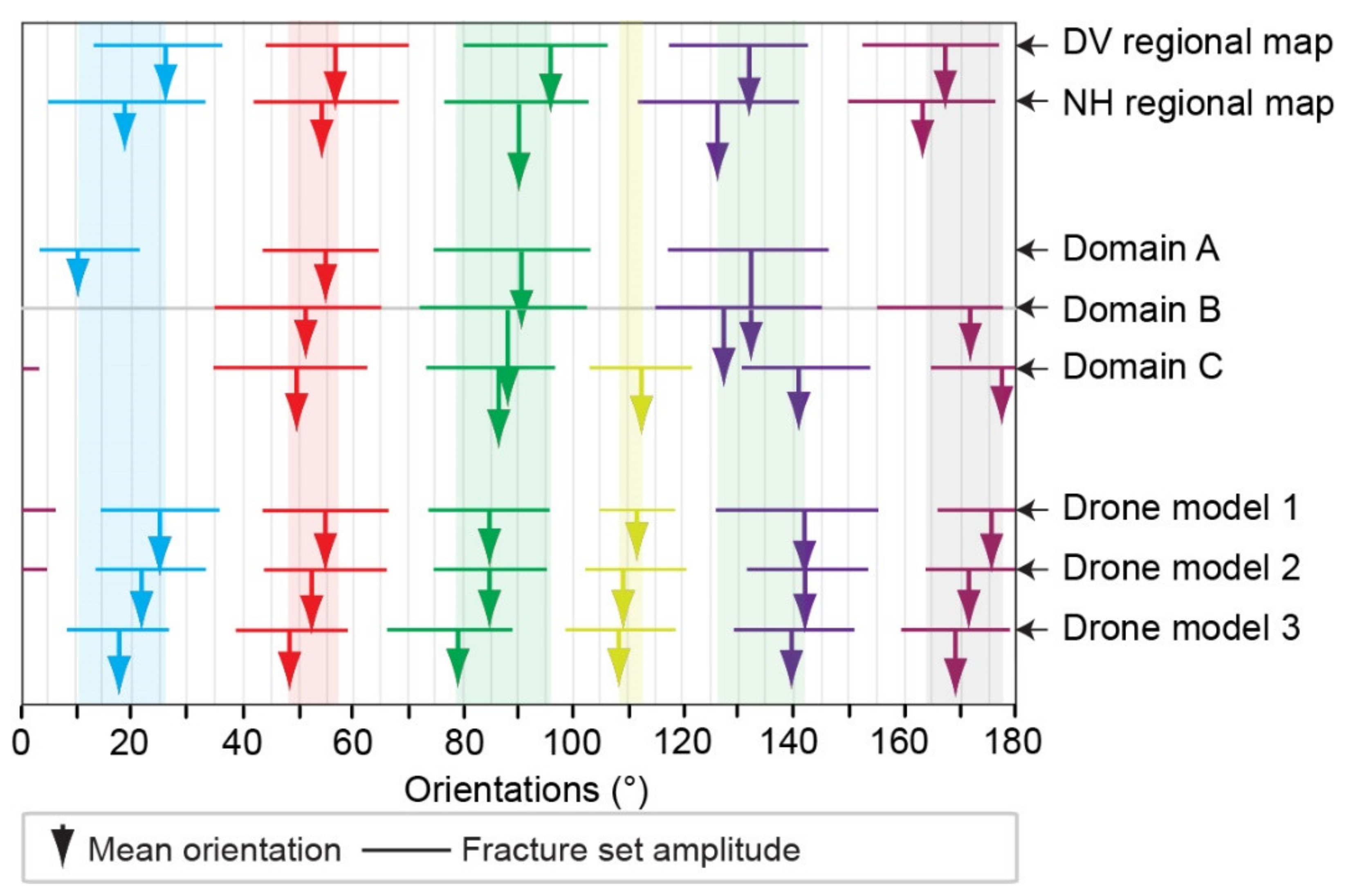
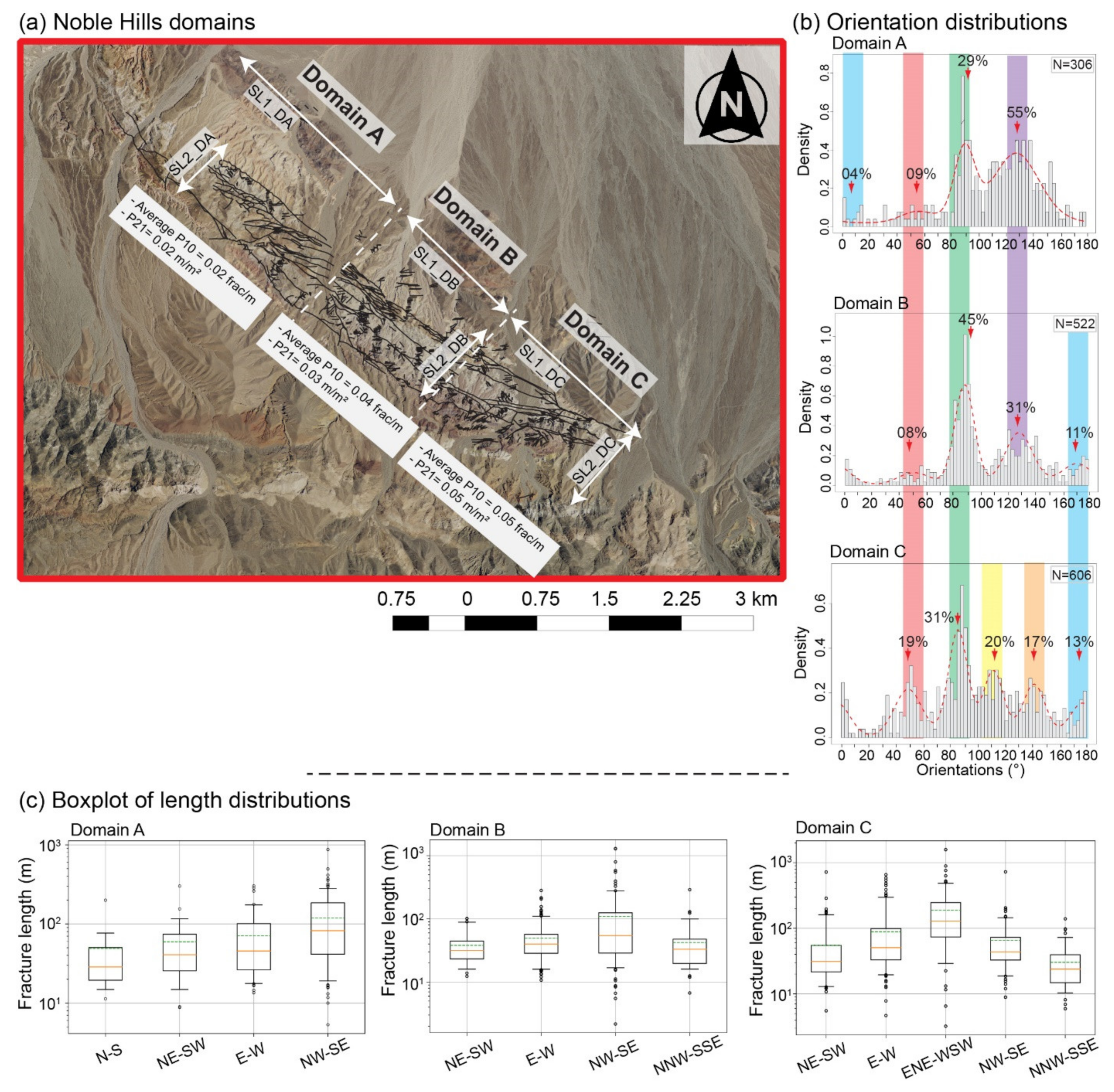
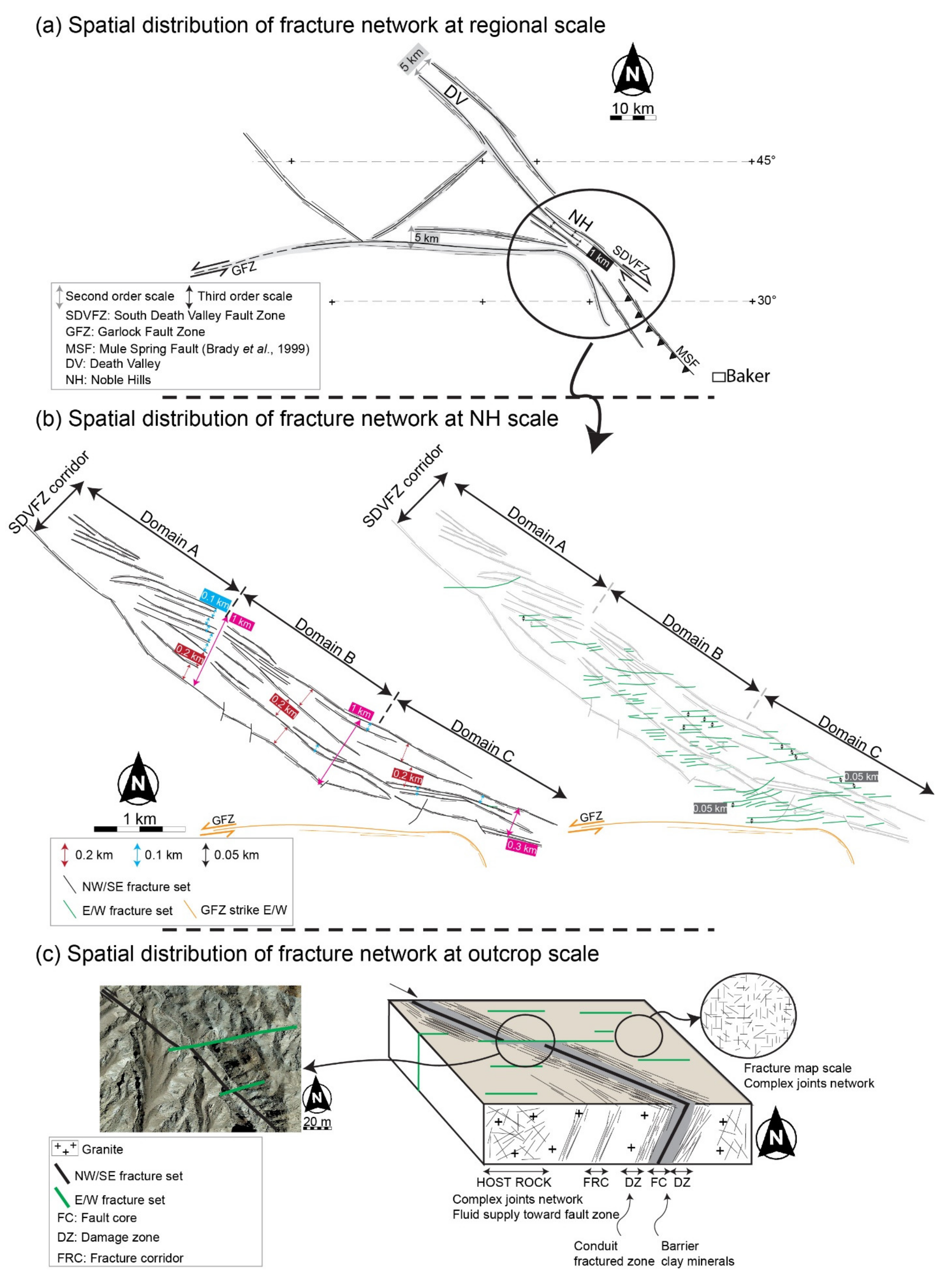
5.2. Spatial Organization of NH Fracture Network
- The first domain referred to the NH domain A is characterized by a specific spatial arrangement with a NW/SE direction dominance (Domain A, Figure 11). This direction is marked by the SDVFZ bordering fault of the strike-slip corridor, and is mostly dominated the NH fracture network in terms of length and abundance. It approved the importance of the NW/SE deformation episode at the fourth order scale. These fractures are the longest ones and also control the internal structuration inside the domain (Figure 12b). The E/W direction is less represented in comparison with domains B and C (Figure 11), but still the second most dominated fracture set, with less control on the NH geometry. Regarding the spacing characteristics, the NW/SE fractures set are regularly spaced from 0.1 to 0.2 km, while the E/W fractures set did not exceed 0.1 km spacing (Figure 12b).
- The central domain (domain B, Figure 3) is characterized by several short segments of fractures. Indeed, the E/W direction is also dominated by short fractures with 60 m mean length, while the NW/SE direction is the second dominated system with long fracture of 100 m mean length (Figure 11). Then, NW/SE and E/W directions control the NH geometry respectively following the third and fourth order scale length. In this case, the spacing related to the third order scale is around 1 km between the SDVFZ bordering faults and regularly spaced at 0.2 km (Figure 12b). A spacing of 0.05 km is defined along the E/W fracture set (Figure 12b).
- The southeastern end area corresponding to the domain C (Figure 3) highlights a specific spatial arrangement with an additional fracture set (yellow color, Figure 11), the longest one with 200 m mean length. Indeed, the NW/SE direction is split into N111° and N141° fracture sets thus highlighting the influence of both NW/SE and E/W deformation episodes in this area. Once again, the E/W direction is more expressed, with a 100 m mean length (Figure 11). The ENE/WSW, E/W and also NW/SE directions control the NH geometry and structuration respectively following the third and fourth order scale. The spacing of 0.3 km defined for the third order scale in domain C between the SDVFZ bordering faults is under the third order spacing characteristic. Indeed, the NW/SE direction has been deviated and then the relative spacing is reduced. Regarding the internal organization, the NW/SE and E/W fractures are also regularly spaced with 0.1–0.2 km and 0.05 km, respectively (Figure 12b).
5.3. Fracture Network Impact on Flow
6. Conclusions
Author Contributions
Funding
Data Availability Statement
Acknowledgments
Conflicts of Interest
References
- Bour, O.; Davy, P. Connectivity of Random Fault Networks Following a Power Law Fault Length Distribution. Water Resour. Res. 1997, 33, 1567–1583. [Google Scholar] [CrossRef]
- Gillespie, D.T. Approximate Accelerated Stochastic Simulation of Chemically Reacting Systems. J. Chem. Phys. 2001, 115, 1716–1733. [Google Scholar] [CrossRef]
- Berkowitz, B. Characterizing Flow and Transport in Fractured Geological Media: A Review. Adv. Water Resour. 2002, 25, 861–884. [Google Scholar] [CrossRef]
- Odling, N.E.; Gillespie, P.; Bourgine, B.; Castaing, C.; Chiles, J.P.; Christensen, N.P.; Fillion, E.; Genter, A.; Olsen, C.; Thrane, L. Variations in Fracture System Geometry and Their Implications for Fluid Flow in Fractured Hydrocarbon Reservoirs. Pet. Geosci. 1999, 5, 373–384. [Google Scholar] [CrossRef]
- Johnston, J.D.; McCaffrey, K.J.W. Fractal Geometries of Vein Systems and the Variation of Scalingrelationships with Mechanism. J. Struct. Geol. 1996, 18, 349–358. [Google Scholar] [CrossRef]
- Geiger, S.; Emmanuel, S. Non-Fourier Thermal Transport in Fractured Geological Media. Water Resour. Res. 2010, 46, W07504. [Google Scholar] [CrossRef]
- Ledésert, B.; Dubois, J.; Genter, A.; Meunier, A. Fractal Analysis of Fractures Applied to Soultz-Sous-Forets Hot Dry Rock Geothermal Program. J. Volcanol. Geotherm. Res. 1993, 57, 1–17. [Google Scholar] [CrossRef]
- Dezayes, C.; Genter, A.; Valley, B. Structure of the Low Permeable Naturally Fractured Geothermal Reservoir at Soultz. Comptes Rendus Géosciences 2010, 343, 517–530. [Google Scholar] [CrossRef] [Green Version]
- Valley, B.; Dezayes, C.; Genter, A.; Maqua, E.; Syren, G. Main Fracture Zones in GPK3 and GPK4 and Cross-Hole Correlations. In Proceedings of the EHDRA Scientific Conference, Soultz-sous-Forêts, France, 17–18 March 2005. [Google Scholar]
- Bour, O.; Davy, P. On the Connectivity of Three-dimensional Fault Networks. Water Resour. Res. 1998, 34, 2611–2622. [Google Scholar] [CrossRef]
- Darcel, C.; Bour, O.; Davy, P.; de Dreuzy, J.R. Connectivity Properties of Two-Dimensional Fracture Networks with Stochastic Fractal Correlation: Connectivity of 2D Fractal Fracture Networks. Water Resour. Res. 2003, 39, 1272. [Google Scholar] [CrossRef]
- Odling, N.E. Scaling and Connectivity of Joint Systems in Sandstones from Western Norway. J. Struct. Geol. 1997, 19, 1257–1271. [Google Scholar] [CrossRef]
- Castaing, C.; Halawani, M.A.; Gervais, F.; Chilès, J.P.; Genter, A.; Bourgine, B.; Ouillon, G.; Brosse, J.M.; Martin, P.; Genna, A. Scaling Relationships in Intraplate Fracture Systems Related to Red Sea Rifting. Tectonophysics 1996, 261, 291–314. [Google Scholar] [CrossRef]
- Marrett, R.; Ortega, O.J.; Kelsey, C.M. Extent of Power-Law Scaling for Natural Fractures in Rock. Geology 1999, 27, 799–802. [Google Scholar] [CrossRef]
- Soliva, R.; Schultz, R.A.; Benedicto, A. Three-dimensional Displacement-length Scaling and Maximum Dimension of Normal Faults in Layered Rocks. Geophys. Res. Lett. 2005, 32, L16302. [Google Scholar] [CrossRef] [Green Version]
- Bertrand, L.; Géraud, Y.; Le Garzic, E.; Place, J.; Diraison, M.; Walter, B.; Haffen, S. A Multiscale Analysis of a Fracture Pattern in Granite: A Case Study of the Tamariu Granite, Catalunya, Spain. J. Struct. Geol. 2015, 78, 52–66. [Google Scholar] [CrossRef]
- Bertrand, L.; Jusseaume, J.; Géraud, Y.; Diraison, M.; Damy, P.-C.; Navelot, V.; Haffen, S. Structural Heritage, Reactivation and Distribution of Fault and Fracture Network in a Rifting Context: Case Study of the Western Shoulder of the Upper Rhine Graben. J. Struct. Geol. 2018, 108, 243–255. [Google Scholar] [CrossRef]
- Ehlen, J. Fractal Analysis of Joint Patterns in Granite. Int. J. Rock Mech. Min. Sci. 2000, 37, 909–922. [Google Scholar] [CrossRef]
- Genter, A.; Castaing, C. Effets d’échelle Dans La Fracturation Des Granites. Comptes Rendus de l’Académie des Sci. Ser. IIA Earth Planet. Sci. 1997, 325, 439–445. [Google Scholar] [CrossRef]
- Le Garzic, E.; de L’Hamaide, T.; Diraison, M.; Géraud, Y.; Sausse, J.; De Urreiztieta, M.; Hauville, B.; Champanhet, J.-M. Scaling and Geometric Properties of Extensional Fracture Systems in the Proterozoic Basement of Yemen. Tectonic Interpretation and Fluid Flow Implications. J. Struct. Geol. 2011, 33, 519–536. [Google Scholar] [CrossRef]
- De Dreuzy, J.-R.; Davy, P.; Bour, O. Hydraulic Properties of Two-dimensional Random Fracture Networks Following Power Law Distributions of Length and Aperture. Water Resour. Res. 2002, 38, 12-1–12-9. [Google Scholar] [CrossRef]
- Davy, P.; Le Goc, R.; Darcel, C.; Bour, O.; de Dreuzy, J.R.; Munier, R. A Likely Universal Model of Fracture Scaling and Its Consequence for Crustal Hydromechanics. J. Geophys. Res. 2010, 115, B10411. [Google Scholar] [CrossRef]
- Hardebol, N.J.; Maier, C.; Nick, H.; Geiger, S.; Bertotti, G.; Boro, H. Multiscale Fracture Network Characterization and Impact on Flow: A Case Study on the Latemar Carbonate Platform. J. Geophys. Res. Solid Earth 2015, 120, 8197–8222. [Google Scholar] [CrossRef]
- McCaffrey, K.J.W.; Sleight, J.M.; Pugliese, S.; Holdsworth, R.E. Fracture Formation and Evolution in Crystalline Rocks: Insights from Attribute Analysis. Geol. Soc. Lond. Spec. Publ. 2003, 214, 109–124. [Google Scholar] [CrossRef]
- Bonnet, E.; Bour, O.; Odling, N.E.; Davy, P.; Main, I.; Cowie, P.; Berkowitz, B. Scaling of Fracture Systems in Geological Media. Rev. Geophys. 2001, 39, 347–383. [Google Scholar] [CrossRef] [Green Version]
- Bour, O.; Davy, P.; Darcel, C.; Odling, N. A Statistical Scaling Model for Fracture Network Geometry, with Validation on a Multiscale Mapping of a Joint Network (Hornelen Basin, Norway). J. Geophys. Res. Solid Earth 2002, 107, ETG 4-1–ETG 4-12. [Google Scholar] [CrossRef]
- Bonneau, F.; Caumon, G.; Renard, P.; Sausse, J. Stochastic Sequential Simulation of Genetic-like Discrete Fracture Networks. Proceeding 32nd Gocad Meeting, Nancy, France. 2012. Available online: https://www.ring-team.org/component/liad/?view=pub&id=2214 (accessed on 3 July 2021).
- de Dreuzy, J.-R.; Méheust, Y.; Pichot, G. Influence of Fracture Scale Heterogeneity on the Flow Properties of Three-Dimensional Discrete Fracture Networks (DFN): 3D Fracture Network Permeability. J. Geophys. Res. 2012, 117, B11207. [Google Scholar] [CrossRef] [Green Version]
- Chabani, A. Analyse Méthodologique et Caractérisation Multi-Échelle Des Systèmes de Fractures à l’interface Socle/Couverture Sédimentaire Application à La Géothermie (Bassin de Valence, SE France). These de Doctorat, Paris Sciences et Lettres (ComUE), Paris, France, 2019. Available online: http://www.theses.fr/2019PSLEM046 (accessed on 3 July 2021).
- Morellato, C.; Redini, F.; Doglioni, C. On the Number and Spacing of Faults. Terra Nova 2003, 15, 315–321. [Google Scholar] [CrossRef]
- Bourbiaux, B.; Basquet, R.; Daniel, J.M.; Hu, L.Y.; Jenni, S.; Lange, G.; Rasolofosaon, P. Fractured Reservoirs Modelling: A Review of the Challenges and Some Recent Solutions. First Break 2005, 23. [Google Scholar] [CrossRef]
- Gillespie, P.; Monsen, E.; Maerten, L.; Hunt, D.; Thurmond, J.; Tuck, D.; Martinsen, O.J.; Pulham, A.J.; Haughton, P.D.W.; Sullivan, M.D. Fractures in Carbonates: From Digital Outcrops to Mechanical Models. Outcrops Revital.—Tools Tech. Appl. Tulsa Okla. SEPM Concepts Sedimentol. Paleontol. 2011, 10, 137–147. [Google Scholar]
- Vollgger, S.A.; Cruden, A.R. Mapping Folds and Fractures in Basement and Cover Rocks Using UAV Photogrammetry, Cape Liptrap and Cape Paterson, Victoria, Australia. J. Struct. Geol. 2016, 85, 168–187. [Google Scholar] [CrossRef]
- Biber, K.; Khan, S.D.; Seers, T.D.; Sarmiento, S.; Lakshmikantha, M.R. Quantitative Characterization of a Naturally Fractured Reservoir Analog Using a Hybrid Lidar-Gigapixel Imaging Approach. Geosphere 2018, 14, 710–730. [Google Scholar] [CrossRef]
- Trullenque, G.; Genter, A.; Leiss, B.; Wagner, B.; Bouchet, R.; Léoutre, E.; Malnar, B.; Bär, K.; Rajšl, I. Upscaling of EGS in Different Geological Conditions: A European Perspective. In Proceedings of the Proceedings 43rd Workshop on Geothermal Reservoir Engineering, Stanford, CA, USA, 12–14 February 2018. [Google Scholar]
- Chabani, A.; Trullenque, G.; Rishi, P.; Pomart, A.; Attali, R.; Sass, I. Modelling of Fractured Granitic Geothermal Reservoirs: Use of Deterministic and Stochastic Methods in Discrete Fracture Networks and a Coupled Processes Modeling Framework. In Proceedings of the Extended Abstract, Reykjavik, Iceland, 2 May 2021. [Google Scholar]
- Klee, J.; Trullenque, G.; Ledésert, B.; Potel, S.; Hébert, R.; Chabani, A.; Genter, A. Petrographic Analyzes of Fractured Granites Used as An Analogue of the Soultz-Sous-Forêts Geothermal Reservoir: Noble Hills, CA, USA. In Proceedings of the Extended Abstract, Reykjavik, Iceland, 26 May 2021. [Google Scholar]
- Jennings, C. Geologic Map of California, Scale 1: 250,000. Olaf P. Jenkins Edition, Long Beach Sheet. Calif. Div. Mines Geol, Serie No 33, List No 6347.033; CA, USA, 1962. Available online: https://www.davidrumsey.com/luna/servlet/detail/RUMSEY~8~1~324920~90093990:Geologic-Map-of-California,-Long-Be?sort=Pub_List_No_InitialSort%2CPub_Date%2CPub_List_No%2CSeries_No (accessed on 3 July 2021).
- Niles, J.H. Post-Middle Pliocene Tectonic Development of the Noble Hills, Southern Death Valley, California. Doctoral Dissertation, San Francisco State University, San Francisco, CA, USA, 2016. [Google Scholar]
- Miller, M.; Pavlis, T. The Black Mountains Turtlebacks: Rosetta Stones of Death Valley Tectonics. Earth-Sci. Rev. 2005, 73, 115–138. [Google Scholar] [CrossRef]
- Pavlis, T.L.; Rutkofske, J.; Guerrero, F.; Serpa, L.F. Structural Overprinting of Mesozoic Thrust Systems in Eastern California and Its Importance to Reconstruction of Neogene Extension in the Southern Basin and Range. Geosphere 2014, 10, 732–756. [Google Scholar] [CrossRef] [Green Version]
- Snow, J.K.; Wernicke, B. Uniqueness of Geological Correlations: An Example from the Death Valley Extended Terrain. Geol. Soc. Am. Bull. 1989, 101, 1351–1362. [Google Scholar] [CrossRef]
- DeCelles, P.G. Late Jurassic to Eocene Evolution of the Cordilleran Thrust Belt and Foreland Basin System, Western U.S.A. Am. J. Sci. 2004, 304, 105–168. [Google Scholar] [CrossRef]
- Walker, J.D.; Burchfiel, B.; Davis, G.A. New Age Controls on Initiation and Timing of Foreland Belt Thrusting in the Clark Mountains, Southern California. Geol. Soc. Am. Bull. 1995, 107, 742–750. [Google Scholar] [CrossRef]
- Stewart, J.H. Possible Large Right-Lateral Displacement along Fault and Shear Zones in the Death Valley-Las Vegas Area, California and Nevada. Geol. Soc. Am. Bull. 1967, 78, 131–142. [Google Scholar] [CrossRef]
- Stewart, J.H. Extensional Tectonics in the Death Valley Area, California: Transport of the Panamint Range Structural Block 80 Km Northwestward. Geology 1983, 11, 153–157. [Google Scholar] [CrossRef]
- Snow, J.K. Cenozoic Tectonism in the Central Basin and Range; Magnitude, Rate, and Distribution of Upper Crustal Strain. Am. J. Sci. 2000, 300, 659–719. [Google Scholar] [CrossRef]
- Brady, R. Cenozoic Geology of the Northern Avawatz Mountains in Relation to the Intersection of the Garlock and Death Valley Fault Zones, San Bernardino County, California. Doctoral Dissertation, University of California, Davis, CA, USA, 1987. [Google Scholar]
- Norton, I. Two-Stage Formation of Death Valley. Geosphere 2011, 7, 171–182. [Google Scholar] [CrossRef]
- Burchfiel, B.C.; Stewart, J.H. “Pull-Apart” Origin of the Central Segment of Death Valley, California. Geol. Soc. Am. Bull. 1966, 77, 439–442. [Google Scholar] [CrossRef]
- Pavlis, T.L.; Trullenque, G. Evidence for 40–41 Km of Dextral Slip on the Southern Death Valley Fault: Implications for the Eastern California Shear Zone and Extensional Tectonics. Geology 2021, 49, 767–772. [Google Scholar] [CrossRef]
- Machette, M.N.; Klinger, R.E.; Knott, J.R.; Wills, C.J.; Bryant, W.A.; Reheis, M.C. A Proposed Nomenclature for the Death Valley Fault System. Quaternary and Late Pliocene Geology of the Death Valley Region: Recent Observations on Tectonics, Stratigraphy, and Lake Cycles (Guidebook for the 2001 Pacific Cell—Friends of the Pleistocene Fieldtrip); US Department of the Interior, US Geological Survey: Reston, VA, USA, 2001; p. 173.
- Troxel, B.W.; Butler, P.R. Rate of Cenozoic Slip on Normal Faults, South-Central Death Valley, California. Doctoral Dissertation, Departement of Geology, University of California, Office of Scholarly Communication (OSC), Irvine, CA, USA, 1979. [Google Scholar]
- Brady III, R.H. Neogene Stratigraphy of the Avawatz Mountains between the Garlock and Death Valley Fault Zones, Southern Death Valley, California: Implications as to Late Cenozoic Tectonism. Sediment. Geol. 1984, 38, 127–157. [Google Scholar] [CrossRef]
- Reinert, E. Low Temperature Thermochronometry of the Avawatz Mountians, California: Implications for the Inception of the Eastern California Shear Zone. Doctoral Dissertation, University of Washington, Washington, DC, USA, 2004. Available online: https://www.ess.washington.edu/content/people/student_publications_files/reinert--erik/Reinert_2004.pdf (accessed on 3 July 2021).
- Spencer, J.E. Late Cenozoic Extensional and Compressional Tectonism in the Southern and Western Avawatz Mountains, Southeastern California. Basin and Range Extensional Tectonics near the Latitude of Las Vegas, Nevada: Geological Society of America Memoir; Geological Society of America: Las Vegas, NV, USA, 1990; Volume 176, pp. 317–333. [Google Scholar] [CrossRef]
- Chinn, L.D. Low-Temperature Thermochronometry of the Avawatz Mountains; Implications for the Eastern Terminus and Inception of the Garlock Fault Zone; University of Washington: Washington, DC, USA; Available online: https://www.ess.washington.edu/content/people/student_publications_files/chinn--logan/chinn--logan_ms_2013.pdf (accessed on 3 July 2021).
- Rämö, T.O.; Calzia, J.P.; Kosunen, P.J. Geochemistry of Mesozoic Plutons, Southern Death Valley Region, California: Insights into the Origin of Cordilleran Interior Magmatism. Contrib. Mineral. Petrol. 2002, 143, 416–437. [Google Scholar] [CrossRef]
- Bisdom, K.; Gauthier, B.D.M.; Bertotti, G.; Hardebol, N.J. Calibrating Discrete Fracture-Network Models with a Carbonate Threedimensional Outcrop Fracture Network: Mplications for Naturally Fractured Reservoir Modeling. AAPG Bull. 2014, 98, 13511376. [Google Scholar] [CrossRef]
- Brady, R.H.; Troxel, B.W.; Wright, L.A. The Miocene Military Canyon Formation: Depocenter Evolution and Constraints on Lateral Faulting, Southern Death Valley, California. Spec. Pap. Geol. Soc. Am. 1999, 277–288. [Google Scholar] [CrossRef]
- von Mises, R. Uber Die “Ganzzahligkeit” Der Atomgewicht Und Verwandte Fragen. Physikal. Z. 1918, 19, 490–500. [Google Scholar]
- Chabani, A.; Mehl, C.; Cojan, I.; Alais, R.; Bruel, D. Semi-Automated Component Identification of a Complex Fracture Network Using a Mixture of von Mises Distributions: Application to the Ardeche Margin (South-East France). Comput. Geosci. 2020, 137, 104435. [Google Scholar] [CrossRef]
- Pickering, G.; Bull, J.M.; Sanderson, D.J. Sampling Power-Law Distributions. Tectonophysics 1995, 248, 1–20. [Google Scholar] [CrossRef] [Green Version]
- Pickering, G.; Peacock, D.C.; Sanderson, D.J.; Bull, J.M. Modeling Tip Zones to Predict the Throw and Length Characteristics of Faults. AAPG Bull. 1997, 81, 82–99. [Google Scholar]
- Davy, P.; Bour, O.; De Dreuzy, J.-R.; Darcel, C. Flow in Multiscale Fractal Fracture Networks. Geol. Soc. Lond. Spec. Publ. 2006, 261, 31–45. [Google Scholar] [CrossRef]
- Ledésert, B.; Dubois, J.; Velde, B.; Meunier, A.; Genter, A.; Badri, A. Geometrical and Fractal Analysis of a Three-Dimensional Hydrothermal Vein Network in a Fractured Granite. J. Volcanol. Geotherm. Res. 1993, 56, 267–280. [Google Scholar] [CrossRef]
- Cruden, D.M. Describing the Size of Discontinuities; Elsevier: Amsterdam, The Netherlands, 1977; Volume 14, pp. 133–137. [Google Scholar]
- Priest, S.D.; Hudson, J.A. Estimation of Discontinuity Spacing and Trace Length Using Scanline Surveys; Elsevier: Amsterdam, The Netherlands, 1981; Volume 18, pp. 183–197. [Google Scholar]
- Priest, S.D.; Hudson, J.A. Discontinuity Spacings in Rock. Int. J. Rock Mech. Min. Sci. Geomech. Abstr. 1976, 13, 135–148. [Google Scholar] [CrossRef]
- Cowie, P.A.; Sornette, D.; Vanneste, C. Multifractal Scaling Properties of a Growing Fault Population. Geophys. J. Int. 1995, 122, 457–469. [Google Scholar] [CrossRef] [Green Version]
- Priest, S.D. Discontinuity Analysis for Rock Engineering; Springer Science & Business Media: Berlin/Heidelberg, Germany, 1993. [Google Scholar]
- Gillespie, C.S. The PoweRlaw Package: A General Overview. Newcastle, UK. Available online: https://cran.r-project.org/web/packages/poweRlaw/vignettes/a_introduction.pdf (accessed on 3 July 2021).
- Gillespie, P.A.; Howard, C.B.; Walsh, J.J.; Watterson, J. Measurement and Characterisation of Spatial Distributions of Fractures. Tectonophysics 1993, 226, 113–141. [Google Scholar] [CrossRef]
- Bertrand, L. Etude Des Réservoirs Géothermiques Développés Dans Le Socle et à l’interface Avec Les Formations Sédimentaires. Doctoral Dissertation, Université de Lorraine, Lorraine, France, April 2017; p. 492. [Google Scholar]


| Nb of Fractures | Mean Orientation | Average SL Length (m)/Area (m²) | Fracture Density (P10) (frac/m) | Fracture Density (P21) (m/m²) | |
|---|---|---|---|---|---|
| DV regional map | 133 | N025 | 105/1.3 × 1010 | 2 × 10⁻⁴ | 3 × 10⁻⁴ |
| 188 | N058 | ||||
| 199 | N096 | ||||
| 248 | N132 | ||||
| 197 | N167 | ||||
| NH regional map | 97 | N020 | 4.7 × 10³/4.4 × 106 | 2.6 × 10⁻⁴ | 3 × 10⁻⁴ |
| 168 | N054 | ||||
| 535 | N090 | ||||
| 441 | N126 | ||||
| 192 | N163 | ||||
| NH domain A | 13 | N010 | 1.5 × 10³/1.9 × 106 | 2 × 10⁻² | 2 × 10⁻² |
| 26 | N055 | ||||
| 89 | N091 | ||||
| 168 | N132 | ||||
| NH domain B | 43 | N050 | 1.7 × 10³/1.2 × 106 | 4 × 10⁻² | 3 × 10⁻² |
| 233 | N088 | ||||
| 164 | N128 | ||||
| 59 | N171 | ||||
| NH domain C | 113 | N049 | 2 × 10³/1.2 × 106 | 5 × 10⁻² | 5 × 10⁻² |
| 191 | N085 | ||||
| 119 | N111 | ||||
| 103 | N141 | ||||
| 77 | N177 | ||||
| Drone model 1 | 235 | N025 | 3.5 × 10²/1.4 × 104 | 6.5 × 10⁻¹ | 2 × 10⁻¹ |
| 208 | N055 | ||||
| 183 | N085 | ||||
| 112 | N115 | ||||
| 281 | N142 | ||||
| 214 | N174 | ||||
| Drone model 2 | 681 | N022 | 1.7 × 10²/5.8 × 103 | 1.28 | 7 × 10⁻¹ |
| 767 | N043 | ||||
| 642 | N085 | ||||
| 616 | N108 | ||||
| 722 | N142 | ||||
| 637 | N171 | ||||
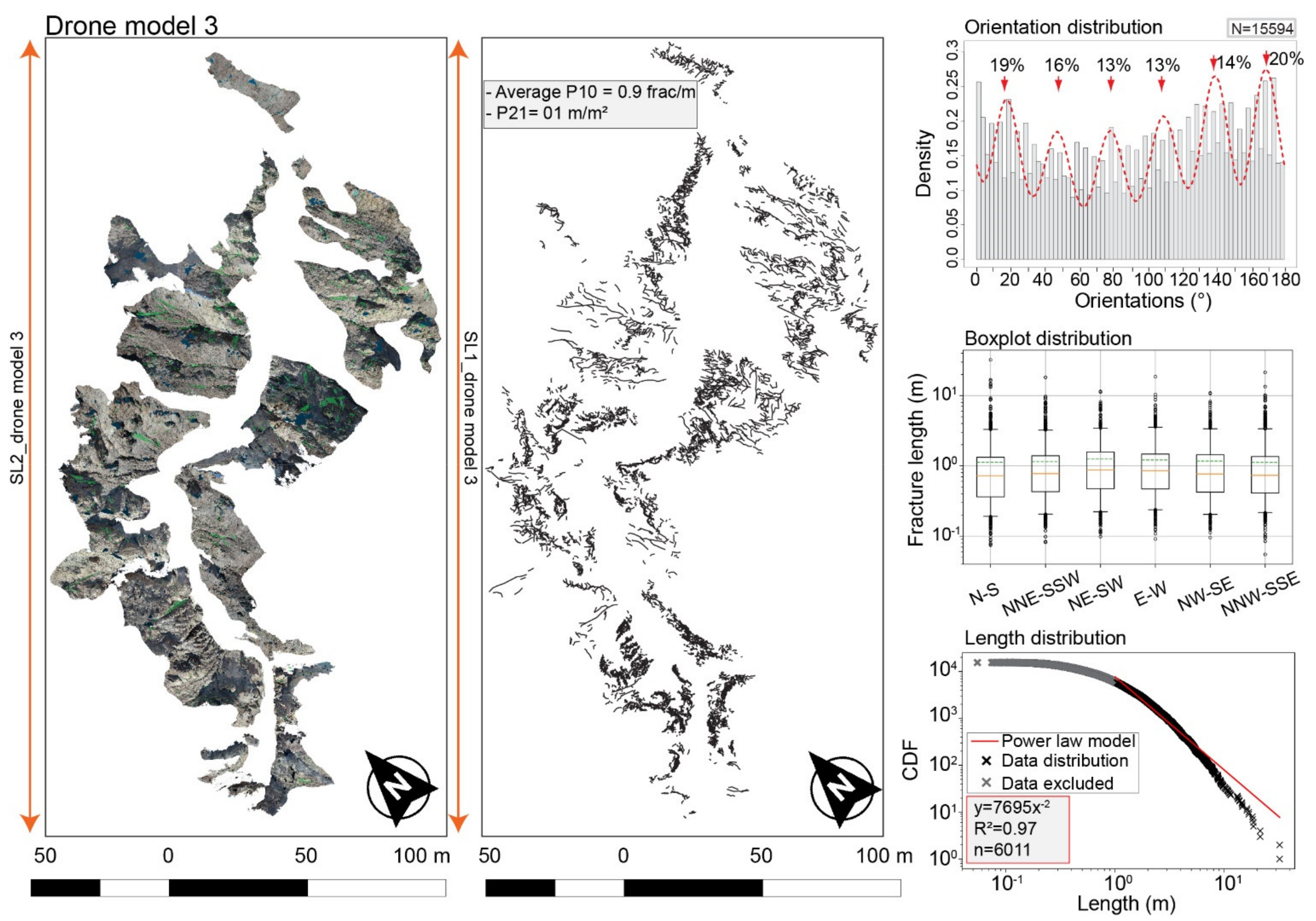
| Drone model 3 | 2968 | N018 | 2.8 × 10²/1.7 × 104 | 9 × 10⁻¹ | 1 |
| 2531 | N038 | ||||
| 1993 | N079 | ||||
| 2127 | N109 | ||||
| 2232 | N140 | ||||
| 3084 | N169 |
| Nb of Fractures | Mean Orientation | Average SL Length (m)/Area (m²) | Fracture Density (P10) (frac/m) | Fracture Density (P21) (m/m²) | |
|---|---|---|---|---|---|
| Fracture map 1 | 1133 | N005 | 3.1/7.94 | 12 | 12 |
| 631 | N083 | ||||
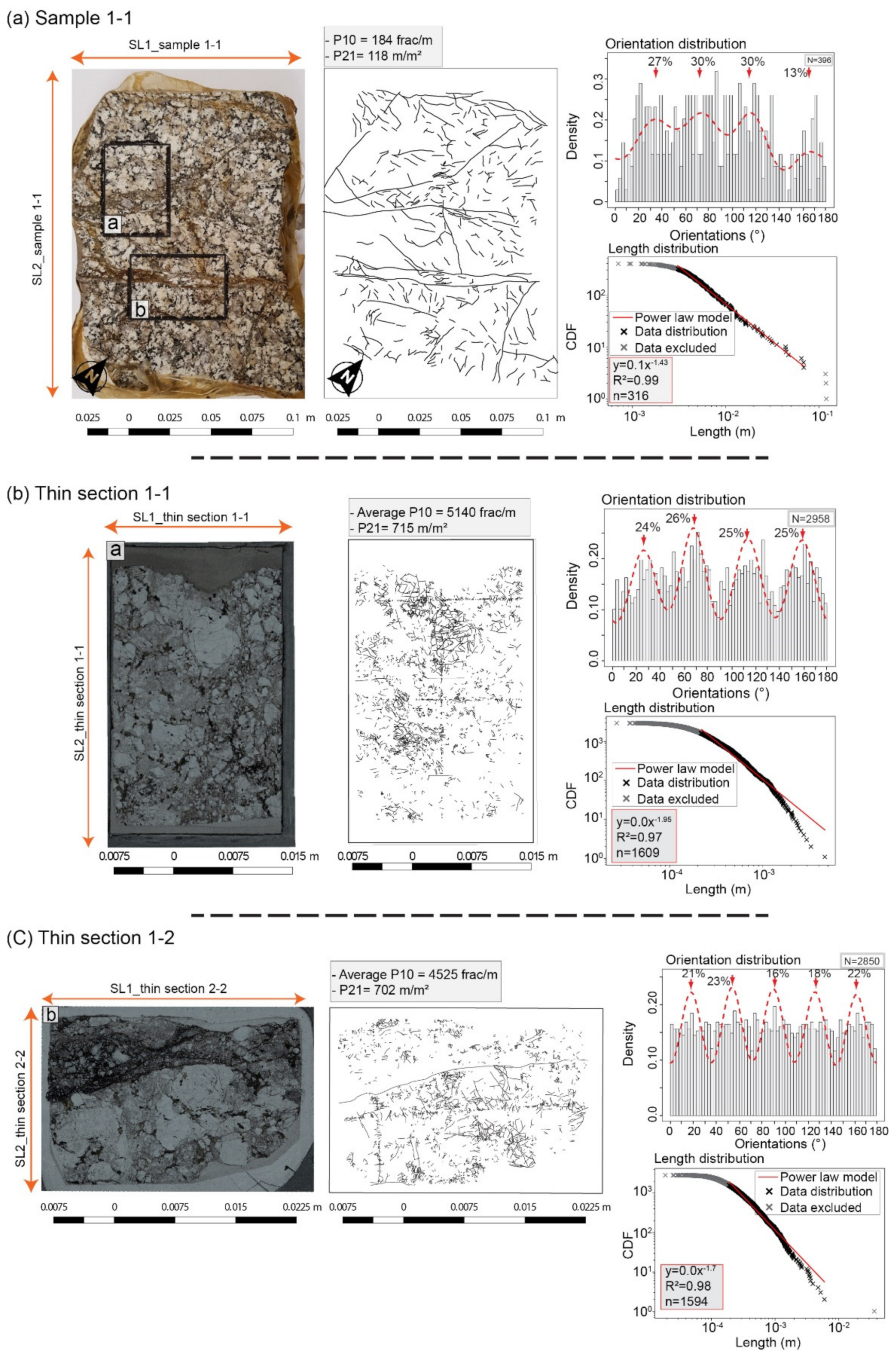
| Sample 1-1 | 104 | N018 | 15 × 10−2/2.2 × 10−2 | 184 | 118 |
| 115 | N053 | ||||
| 117 | N090 | ||||
| 51 | N126 | ||||
| Thin section 1-1 | 723 | N018 | 3 × 10⁻²/8 × 10−4 | 5140 | 715 |
| 754 | N053 | ||||
| 751 | N090 | ||||
| 730 | N126 | ||||
| Thin section 1-2 | 612 | N020 | 3 × 10⁻²/8 × 10−4 | 4525 | 702 |
| 659 | N051 | ||||
| 444 | N088 | ||||
| 512 | N128 | ||||
| 623 | N162 | ||||
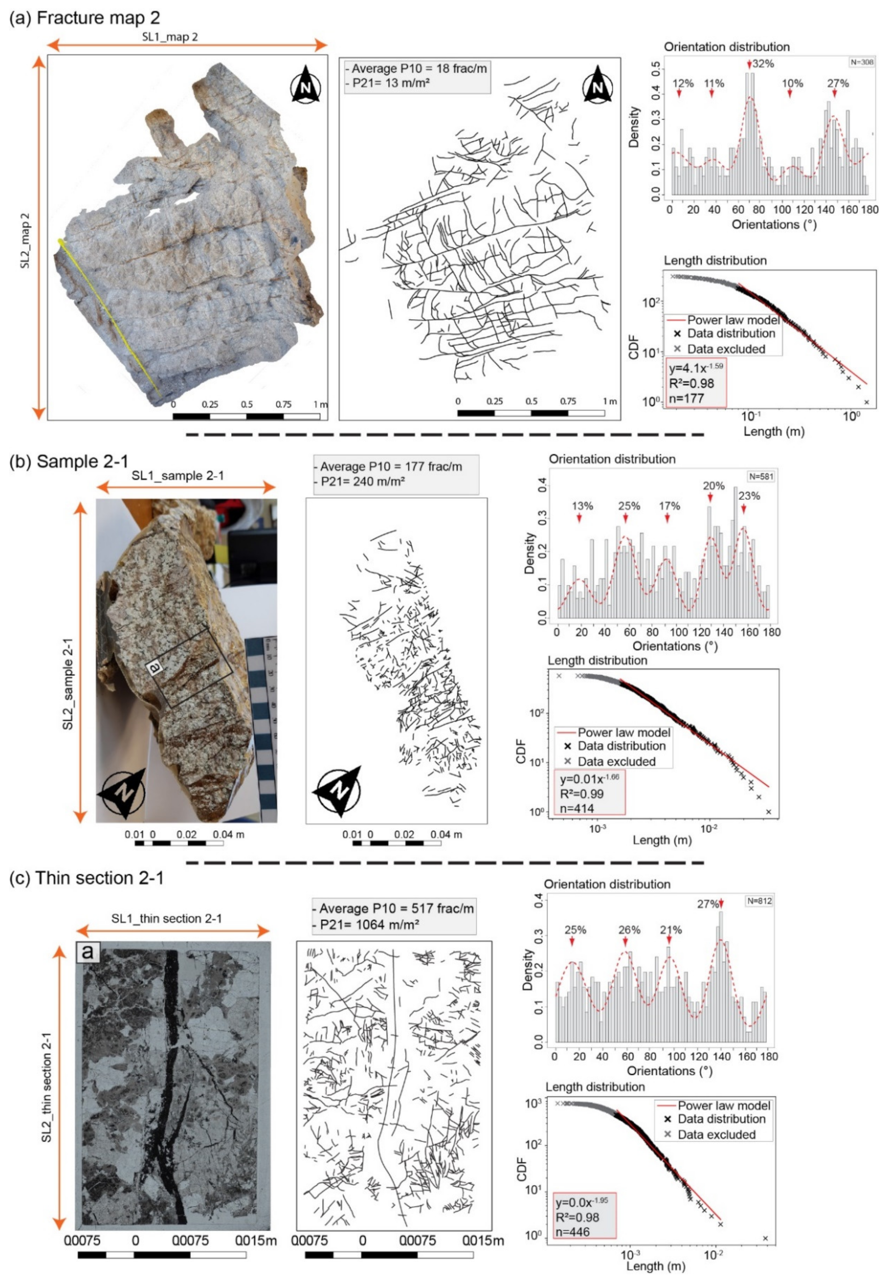
| Fracture map 2 | 36 | N005 | 1.7/1.91 | 18 | 13 |
| 34 | N038 | ||||
| 98 | N070 | ||||
| 32 | N110 | ||||
| 83 | N145 | ||||
| Sample 2-1 | 75 | N017 | 10−1/10−2 | 177 | 240 |
| 145 | N057 | ||||
| 101 | N092 | ||||
| 116 | N130 | ||||
| 135 | N157 | ||||
| Thin section 2-1 | 201 | N014 | 3 × 10⁻²/8 × 10−4 | 517 | 1064 |
| 213 | N059 | ||||
| 170 | N097 | ||||
| 221 | N140 | ||||
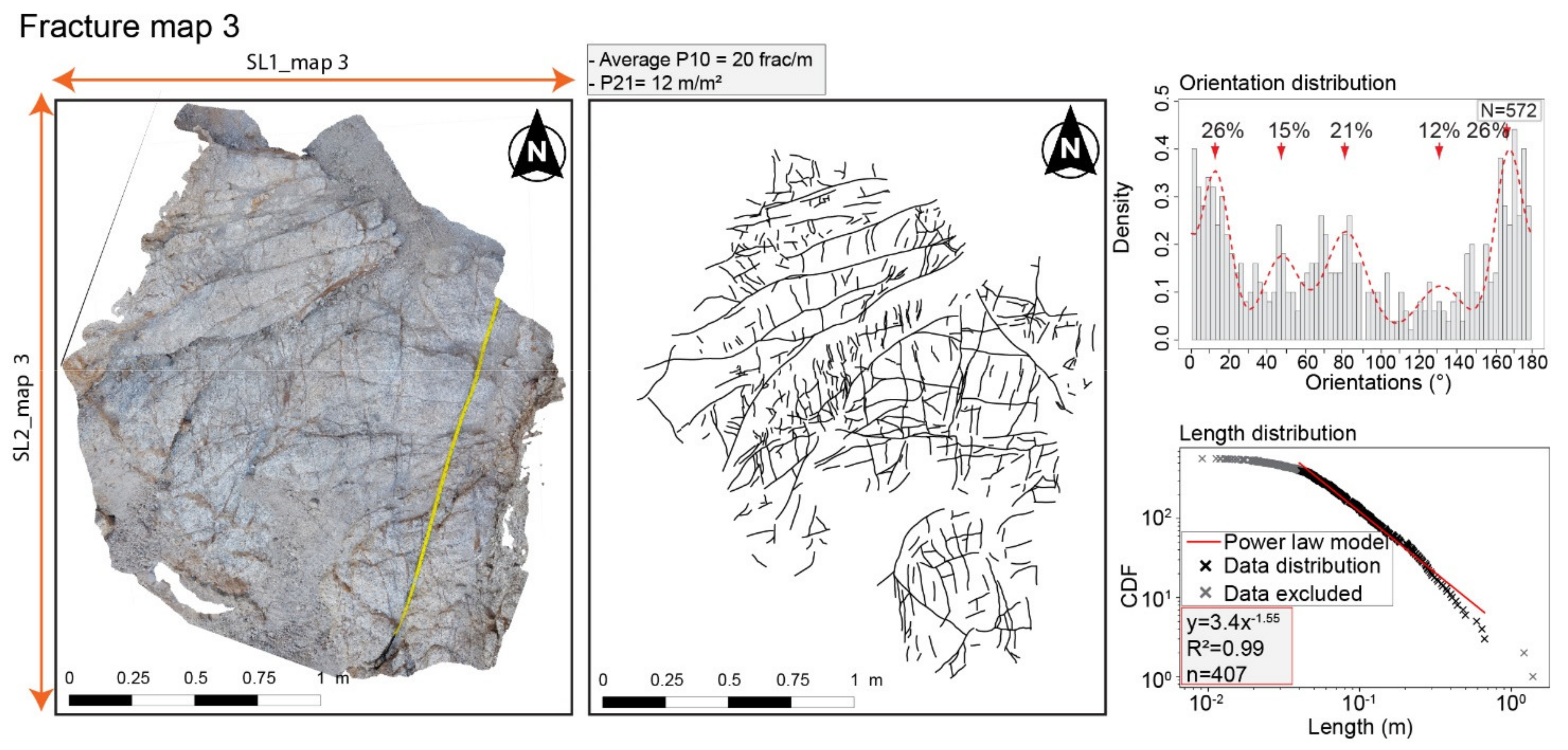
| Fracture map 3 | 149 | N009 | 1.7/3 | 20 | 12 |
| 88 | N033 | ||||
| 119 | N071 | ||||
| 70 | N104 | ||||
| 146 | N149 |
Publisher’s Note: MDPI stays neutral with regard to jurisdictional claims in published maps and institutional affiliations. |
© 2021 by the authors. Licensee MDPI, Basel, Switzerland. This article is an open access article distributed under the terms and conditions of the Creative Commons Attribution (CC BY) license (https://creativecommons.org/licenses/by/4.0/).
Share and Cite
Chabani, A.; Trullenque, G.; Ledésert, B.A.; Klee, J. Multiscale Characterization of Fracture Patterns: A Case Study of the Noble Hills Range (Death Valley, CA, USA), Application to Geothermal Reservoirs. Geosciences 2021, 11, 280. https://doi.org/10.3390/geosciences11070280
Chabani A, Trullenque G, Ledésert BA, Klee J. Multiscale Characterization of Fracture Patterns: A Case Study of the Noble Hills Range (Death Valley, CA, USA), Application to Geothermal Reservoirs. Geosciences. 2021; 11(7):280. https://doi.org/10.3390/geosciences11070280
Chicago/Turabian StyleChabani, Arezki, Ghislain Trullenque, Béatrice A. Ledésert, and Johanne Klee. 2021. "Multiscale Characterization of Fracture Patterns: A Case Study of the Noble Hills Range (Death Valley, CA, USA), Application to Geothermal Reservoirs" Geosciences 11, no. 7: 280. https://doi.org/10.3390/geosciences11070280
APA StyleChabani, A., Trullenque, G., Ledésert, B. A., & Klee, J. (2021). Multiscale Characterization of Fracture Patterns: A Case Study of the Noble Hills Range (Death Valley, CA, USA), Application to Geothermal Reservoirs. Geosciences, 11(7), 280. https://doi.org/10.3390/geosciences11070280