Abstract
The mechanical characterization of biological samples is a fundamental issue in biology and related fields, such as tissue and cell mechanics, regenerative medicine and diagnosis of diseases. In this paper, a novel approach for the identification of the stiffness and damping coefficients of biosamples is introduced. According to the proposed method, a MEMS-based microgripper in operational condition is used as a measurement tool. The mechanical model describing the dynamics of the gripper-sample system considers the pseudo-rigid body model for the microgripper, and the Kelvin–Voigt constitutive law of viscoelasticity for the sample. Then, two algorithms based on recursive least square (RLS) methods are implemented for the estimation of the mechanical coefficients, that are the forgetting factor based RLS and the normalised gradient based RLS algorithms. Numerical simulations are performed to verify the effectiveness of the proposed approach. Results confirm the feasibility of the method that enables the ability to perform simultaneously two tasks: sample manipulation and parameters identification.
1. Introduction
The mechanical characterization of biomaterials represents a crucial procedure in the fields of tissue engineering, tissue and cell mechanics, disease diagnosis and minimally invasive surgery (MIS) [1,2,3].
For instance, modeling the mechanical response of brain tissue can be useful in the understanding of traumatic brain injury [4] or blast–induced neurotrauma [5] mechanisms. In tissue engineering, scaffolds should achieve appropriate mechanical properties in order to ensure tissue growth. Therefore, before implantation, it is necessary to verify if these properties meet the specified requirements [6,7]. Many investigations have also been focused on the characterization and on the constitutive modeling of skin [8,9], cornea [10], vocal fold [11], skeletal muscle [12], and blood vessels [1] tissues. Regarding the circulatory system, it is worth mentioning that vascular stiffness is recognized as an important factor in diseases such as pulmonary arterial hypertension, kidney disease, and atherosclerosis [13]. Generally, the variation of tissue stiffness is a hallmark of several disease states, including fibrosis and some types of cancers [14]. Viscosity can also be considered as a biomarker for the metastatic potential of cancer cells [15,16], and the analysis of both elastic and viscous properties could be more effective in detecting and identifying specific diseases [17].
The characterization of the mechanical properties of biomaterials is important not only for in vitro analysis. For example, in MIS operations, tactile information is not available to the surgeon. Therefore, the capability of on-line detecting and identifying tissues could play a fundamental role in the advancement of MIS procedures [3].
The mechanical properties of tissues have been investigated by using various methods, such as indentation and aspiration, and measuring deformations by means of ultrasound or magnetic resonance imaging techniques [18]. Surgical instruments have also been improved with sensing capabilities [19]. For example, a micro-tactile MEMS-based sensor to be integrated within MIS graspers was presented in Reference [3], whereas a sensor capable of determining the stiffness of biological tissues was modeled and tested in Reference [20].
At the cell level, experimental techniques for investigating mechanical properties include force-application techniques (e.g., micropipette aspiration, atomic force microscope probing, optical trapping), and force-sensing techniques (e.g., traction force microscopy, wrinkling membranes, micropost arrays). The technique selection depends on size of the biological sample, feature to be acquired, detrimental effects on the sample, spatial and force resolution, and accuracy [21,22].
Given the large number of experimental approaches, many mechanical models have been proposed in literature, based on the micro/nanostructural approach and on the continuum approach. The former model targets the sub-cell level, whereas the latter one treats the biological sample as a continuum material. Considering the continuum approach, many constitutive models have been proposed in literature, such as biphasic model, liquid drop models, solid viscoelastic models (Kelvin–Voigt, Maxwell, Zener) [23,24]. Once the mathematical model is available, a parameter estimation problem can be formulated and solved by means of different methods, such as least-squares [25], Kalman filtering [26], or inverse finite element [18,27] methods.
In the last decade, microgrippers became essential tools in the manipulation at the microscale [28,29,30,31,32,33], and can be adopted to develop novel techniques for the viscoelastic characterization of soft materials. In their previous investigation [34], the Authors proposed a method to evaluate the mechanical properties of a biomaterial sample based on the use of a MEMS microgripper. The mechanical model was developed considering the gripper–sample kinematics and the Kelvin–Voigt constitutive law of viscoelasticity, and a PID controller to determine stiffness and viscous parameters of the sample.
In this work, a parameter estimation problem is formulated starting from the model presented in Reference [34]. Recursive least squares filtering algorithms are implemented to characterize the mechanical properties of soft biomaterials, enabling the on-line identification of stiffness and viscosity coefficients. With respect to the other experimental techniques briefly mentioned above, that generally are implemented only for the mechanical testing procedure, the proposed approach enables the ability to perform the mechanical characterization while the sample is manipulated for a different purpose in another operation. Furthermore, this method does not require additional elements other than the measurement tool and the specimen as, for example, beads used with optical tweezers. Also, risks related to laser-induced damage and to large deformations of the sample (involved in optical traps and micropipette aspiration, respectively) are avoided.
2. The Experimental Device
The microsystem considered in this paper consists of two silicon arms actuated by rotary comb drives, as shown in Figure 1. The electrostatic actuators exert the input torques that, through the conjugate surface flexure hinges (CSFH) deflections [35,36], move the arms from the initial position to perform the gripping task [37]. In the neutral configuration, the distance between the jaws is equal to 150 m. The fabrication method relies on the application of deep reactive-ion etching on silicon-on-insulator wafers [38].
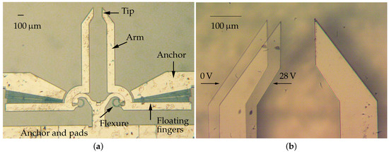
Figure 1.
Optical microscope images of the device. The whole microgripper (a) and two overlapping frames showing the left arm in neutral (0 V) and actuated (28 V) configurations (b).
In their previous investigations [34,39], the authors estimated the mechanical characteristic of the sample considering input signals of suitable waveform. According to the proposed method, the sample is gripped with the left arm until the right arm reaches a predefined rotation, that serves as a reference signal for the implemented feedback control scheme. Therefore, the stiffness coefficient can be computed at steady state conditions [39]. In order to estimate also the sample viscosity, a small-amplitude sinusoidal signal was added to the left arm, and the viscous coefficient was obtained as a function of the input torque frequency [34].
In this paper, an estimation algorithm for the elastic and viscosity parameters of the gripped sample under generic control torques is presented. As demonstrated in the next Sections, the algorithm take advantage of the mathematical model structure that, despite its general non linearity, is linear with respect to the unknown parameters.
3. The Mathematical Model
In operative condition, the microdevice is gripping a sample between its jaws, as illustrated in Figure 2. More specifically, Figure 2a shows a schematic drawing of the compliant structure of the gripper. The contact points between jaws and sample are labelled as B and C, whereas the points A and D represent the centers of rotation of the left and right arms, respectively. Starting from the compliant mechanism, a pseudo-rigid body model (PRBM) can be obtained by substituting the constant-curvature CSFHs with revolute joints [35,40,41,42]. Figure 2b shows the PRBM of the microgripper: the quadrilateral is a closed chain composed by the links (frame), and (arms), and (sample). All the links have a fixed length with the exception of , whose compression is at the basis of the measurement procedure. The proposed model takes into account the nonlinearity related to the kinematics of the gripper, but it assumes a linear behavior for stiffness coefficients and . Moreover, the identification of the cell parameters inherently assumes that its dynamic behavior can be described by the Kelvin–Voight constitutive model of viscoelasticity.
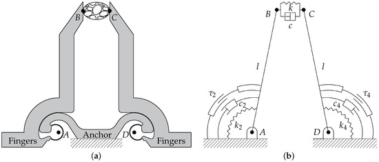
Figure 2.
Schematic representations of the microgripper: compliant mechanism (a) and corresponding pseudo-rigid body model (b).
With reference to Figure 2b, the following parameters can be introduced:
- l is the common length of the two links representing the arms, i.e., the distances and ;
- d is the distance between the hinges (), i.e., the frame length;
- , and k are the torsional stiffness of the two arms hinges and the stiffness of the sample, respectively;
- , and c are the viscous damping coefficients of the two arms and of the sample, respectively;
- and are the moments of inertia of the left and right arms around A and D, respectively;
- and are the input torques generated by the left and right comb drives, respectively.
For the sake of simplicity in the model representation, all the considered variables are referred to the neutral layout: the gripper, in symmetrical configuration, is in contact with the sample but no deformation occurs. By following the notation introduced in Reference [34], and with reference to Figure 3a, the angles , , and represent the reference orientations of the links , and , respectively, whereas represents the reference length of the link . The notation is used for the parameters in the deformed configuration, as shown in Figure 3b. Therefore, the angles represent the relative angular displacements of the two links from their neutral configuration, with for the left link and for the right one. The orientation of follows the same notation, with and , whereas the deformation is equal to . The values of the variables in the neutral configuration are given in Table 1.
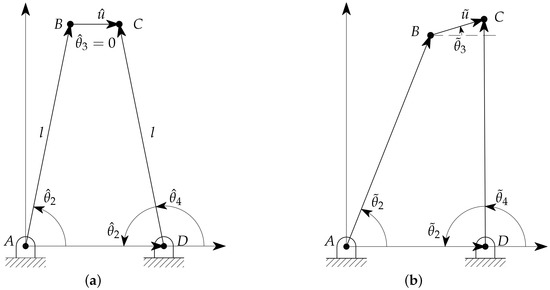
Figure 3.
Nomenclature and model parameters in neutral (a) and general (b) configurations.

Table 1.
Constants.
Assuming the inertia of the sample to be negligible, the dynamical model of the links can be written as
where the subscripts 2 and 4 refer to the left and right joints, respectively. For the device here considered, the values of the parameters appearing in (1) and (2) are reported in Table 2.
Table 2.
Numerical values of the parameters.
4. Mechanical Characteristics Estimation
As briefly described in the Introduction, an approach to determine both the elastic and viscous characteristics of a biosample by using a microgripper was proposed in Reference [34], where particular waveforms were required for the input torques. However, this method is not suitable to perform simultaneous manipulation and measurement tasks.
To overcome this limitation, a measurement scheme adaptable to various operative conditions should be considered. Therefore, an on-line dynamical estimator could be implemented as a more efficient strategy for the mechanical characterization of the sample. Recursive least square methods can be successfully applied when the unknown parameters are the linear coefficients of the system dynamic equations. In such cases, quite usual in literature [43,44,45,46], the model can be rearranged as a linear time-varying system with respect to the parameters to be estimated, whereas the other terms, supposed measurable, are functions either of the state or of the output variables.
The model dynamics has to be rearranged as
where m is the number of degrees of freedom of the system ( in the considered case), is the vector of unknown parameters, and , are known quantities depending on the system dynamics. It is worth noting that all the terms in Equation (6) are time dependent.
Equations (1) and (2) can be rewritten, according to the notation in Equation (6), in linear form with respect to the parameters as
where the sign in Equation (8) is minus or plus if or if , respectively.
Referring to Equations (7)–(9), the general expressions to be defined for a generic recursive last squares (RLS) filtering algorithm are [47]:
where and are the current estimation values of and , is the current prediction error, is the gain determining how much the prediction error affects the update in the parameters estimation, and represents the gradient of the predicted model output with respect to .
Two recursive last squares (RLS) filtering algorithms are applied considering different ranges of values for the parameters to be estimated. The algorithms are then compared to each other to understand how much the different viscous and elastic characteristics of the dynamical system affects the convergence of the estimation algorithms. With respect to the formulation in Equation (10), the two approaches differ for the choice of . Moreover, it is worth noting that the symmetric structure of the dynamics represented by Equations (1) and (2) implies that, under a full state measurement, the results obtained choosing are equal to the results corresponding to the case . Therefore, firstly the case and consecutively the case are addressed. Once equivalence and effectiveness of both cases has been proved, the choice in real applications should be driven by the simplicity of the measurement. For example, the operative technique of torque action on the first jaw only implies that for no torque measurement is required, strongly simplifying the implementation.
4.1. Forgetting Factor Based RLS
The first method is based on a forgetting factor based RLS algorithm. In Equation (10), the following choice is performed
where
and
It’s assumed that the residual (the difference between the estimated and the measured value of ) is affected by a white noise with covariance equal to 1. According to previous equations, is computed in order to minimize the sum of residuals squares
In Equations (11)–(14), is the forgetting factor introduced in order to consider differently the time sequence of the errors , according to an exponentially decreasing weight if . This choice is effective in case of time varying parameters while, when dealing with constant parameters, the choice is usually adopted.
The algorithm in Equation (10), with positions (11)–(13), has been applied to the case . In all the simulations, the initial values of the parameters have been chosen far from the real values. The initial covariance, proportional to , has been fixed taking into account that the covariance matrix has to be chosen according to a priori knowledge of the parameters at : very high values of the covariance matrix elements correspond to completely unknown parameters.
Remark 1.
Note that the forgetting factor method is a particular simplified case of the Kalman filter.
4.2. Normalised Gradient Based RLS
The second approach consists of a normalized gradient algorithm. This technique is based on the choice of with a simpler form with respect to (11):
where is the adaptation gain scaled by the gradient . The bias term is added to the square norm of the gradient vector in the denominator of the expression, in order to prevent critical situations in the case is close to zero. The algorithm (10) with defined by (15) requires only the initialization for the values of the parameters to be estimated.
Since the presence of noise is not explicitly considered in this formulation, the drawback is a smaller rate of convergence and a larger sensitivity to the presence of noises.
This technique has been simulated making reference to the dynamics represented by Equation (2), that is with .
5. Simulations
Numerical simulations, using Matlab® (MathWorks, Inc., Natick, MA, USA) and Simulink® (MathWorks, Inc., Natick, MA, USA) tools, were performed in order to show effectiveness, benefits and differences of the proposed estimation methods. Three different numerical cases were analysed, considering predominant elastic or dissipative behaviours.
The first case corresponds to a realistic condition with elastic and damping coefficient much greater than the ones of the mechanical structure, with Nms/rad and Nm/rad, where the elastic coefficient greater than the damping one.
In the second case, a damping coefficient greater than the elastic one was considered in order to check, by comparison, the dependency of the algorithm convergence from the two different mechanical characteristics. The order of magnitude for the two coefficients have been exchanged, setting Nms/rad and Nm/rad.
In the last case, a very poorly damped sample has been chosen with Nms/rad, whereas Nm/rad.
The initial parameters values, for all the simulations and for both the estimation algorithms have been chosen as Nms/rad and Nm/rad.
For the forgetting factor RLS estimator introduced in SubSection 4.1, the square covariance matrix is diagonal, with both the diagonal elements equal to , while the forgetting factor is fixed to .
For the normalized gradient estimator, presented in SubSection 4.2, the adaptation gain has been set as and the normalization bias has been chosen as .
Simulation results obtained for the first case ( Nms/rad and Nm/rad) are depicted in Figure 4a for the elastic coefficient k and in Figure 4b for the damping coefficient c. The solid line shows the estimation evolution with the first algorithm, whereas the dashed one reports the results of the second algorithm. The dotted line corresponds to the true values of the parameters, plotted as a reference. As expected, both the algorithms converge in a very short time, but the first is faster than the second.
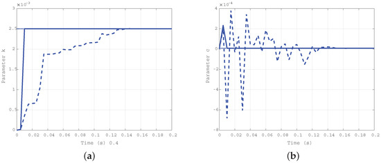
Figure 4.
Time evolution of the estimated parameters k (a) and c (b) for the first case: Nms/rad, Nm/rad.
For the second case ( Nms/rad and Nm/rad), the simulation results are depicted in Figure 5a for the damping coefficient c, and in Figure 5b for the elastic one k. As in the previous case, the solid line refers to the estimation evolution with the first algorithm, the dashed one refers to the second algorithm, and the dotted one is the true reference value. The difference in the convergence rate for the two approaches is confirmed.
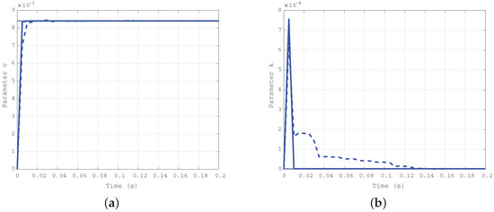
Figure 5.
Time evolution of the estimated parameters c (a) and k (b) for the second case: Nms/rad, Nm/rad.
The results obtained by simulation of the third case ( Nms/rad and Nm/rad) are reported in Figure 6a for the elastic coefficient k, and in Figure 6b for the damping one c. The difference in the convergence rate for the two approaches is confirmed, and uniformity in the estimation of the damping coefficient c with the two algorithms is the same as in the first case.
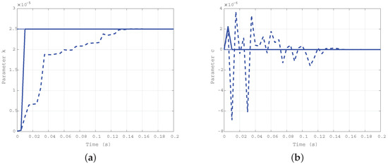
Figure 6.
Time evolution of the estimated parameters k (a) and c (b) for the third case: Nms/rad, Nm/rad.
Numerical results support the effectiveness of the proposed method, tested considering different orders of magnitude for the parameters to be estimated. Clearly, in the present formulation, the state is assumed to be measurable, with possible additive Gaussian noise to model uncertainties and measurement noise.
6. Conclusions
In this paper, the possibility of using a microgripper for the identification of the mechanical properties of biomaterials was investigated. To describe the gripper–sample system dynamics, the pseudo-rigid body model and the Kelvin–Voigt constitutive law of viscoelasticity were considered for the microgripper and for the sample, respectively. The normalised gradient-based RLS and the forgetting factor based RLS algorithms were implemented to solve the parameters estimation problem. Three cases were analysed, assuming different ranges of values for the coefficients to be estimated. The simulation results confirmed the feasibility of the method: both the algorithms converged in a very short time, but the normalised gradient-based RLS algorithm resulted to be faster than the other one. Therefore, the proposed approach could enable the ability to simultaneously perform the manipulation of the biosample and the identification of its mechanical characteristics, i.e., stiffness and damping coefficients. However, the application of the proposed method to a variety of biological samples is limited by the assumption of the Kelvin–Voigt constitutive law of viscoelasticity. From the methodological point of view, further investigations will focus on the implementation of more complex constitutive models and on the design of high-performance algorithms, always attaining robustness with respect to noise and parameter uncertainties.
Author Contributions
P.D.G. and M.L.A. implemented the estimation algorithms and performed the simulations. O.G. and M.V. developed the model adopted for the kinematic and dynamic analysis of the system. All authors contributed in writing the manuscript.
Funding
This research received no external funding.
Acknowledgments
The Authors acknowledge the Micro Nano Facility, Center for Materials and Microsystems of Fondazione Bruno Kesler (FBK-CMM-MNF) for the fabrication of the device and the technical support (Figure 1).
Conflicts of Interest
The authors declare no conflict of interest.
References
- Backman, D.E.; LeSavage, B.L.; Shah, S.B.; Wong, J.Y. A Robust Method to Generate Mechanically Anisotropic Vascular Smooth Muscle Cell Sheets for Vascular Tissue Engineering. Macromol. Biosci. 2017, 17. [Google Scholar] [CrossRef] [PubMed]
- Mijailovic, A.S.; Qing, B.; Fortunato, D.; Van Vliet, K.J. Characterizing viscoelastic mechanical properties of highly compliant polymers and biological tissues using impact indentation. Acta Biomater. 2018, 71, 388–397. [Google Scholar] [CrossRef] [PubMed]
- Qasaimeh, M.; Sokhanvar, S.; Dargahi, J.; Kahrizi, M. A micro-tactile sensor for in situ tissue characterization in minimally invasive surgery. Biomed. Microdevices 2008, 10, 823–837. [Google Scholar] [CrossRef] [PubMed]
- Zhang, W.; Liu, L.F.; Xiong, Y.J.; Liu, Y.F.; Yu, S.B.; Wu, C.W.; Guo, W. Effect of in vitro storage duration on measured mechanical properties of brain tissue. Sci. Rep. 2018, 8, 1247. [Google Scholar] [CrossRef] [PubMed]
- Laksari, K.; Assari, S.; Seibold, B.; Sadeghipour, K.; Darvish, K. Computational simulation of the mechanical response of brain tissue under blast loading. Biomech. Model. Mechanobiol. 2015, 14, 459–472. [Google Scholar] [CrossRef] [PubMed]
- Vivanco, J.; Aiyangar, A.; Araneda, A.; Ploeg, H.L. Mechanical characterization of injection-molded macro porous bioceramic bone scaffolds. J. Mech. Behav. Biomed. Mater. 2012, 9, 137–152. [Google Scholar] [CrossRef] [PubMed]
- Prasadh, S.; Wong, R.C.W. Unraveling the mechanical strength of biomaterials used as a bone scaffold in oral and maxillofacial defects. Oral Sci. Int. 2018, 15, 48–55. [Google Scholar] [CrossRef]
- Edsberg, L.E.; Cutway, R.; Anain, S.; Natiella, J.R. Microstructural and mechanical characterization of human tissue at and adjacent to pressure ulcers. J. Rehabil. Res. Dev. 2000, 37, 463–471. [Google Scholar] [PubMed]
- Hsu, C.K.; Lin, H.H.; Hans, I.; Harn, C.; Hughes, M.; Tang, M.J.; Yang, C.C. Mechanical forces in skin disorders. J. Dermatol. Sci. 2018, 90, 232–240. [Google Scholar] [CrossRef] [PubMed]
- Whitford, C.; Movchan, N.V.; Studer, H.; Elsheikh, A. A viscoelastic anisotropic hyperelastic constitutive model of the human cornea. Biomech. Model. Mechanobiol. 2018, 17, 19–29. [Google Scholar] [CrossRef] [PubMed]
- Erath, B.D.; Zañartu, M.; Peterson, S.D. Modeling viscous dissipation during vocal fold contact: the influence of tissue viscosity and thickness with implications for hydration. Biomech. Model. Mechanobiol. 2017, 16, 947–960. [Google Scholar] [CrossRef] [PubMed]
- Garcés-Schröder, M.; Metz, D.; Hecht, L.; Iyer, R.; Leester-Schädel, M.; Böl, M.; Dietzel, A. Characterization of skeletal muscle passive mechanical properties by novel micro-force sensor and tissue micro-dissection by femtosecond laser ablation. Microelectron. Eng. 2018, 192, 70–76. [Google Scholar] [CrossRef]
- Huveneers, S.; Daemen, M.J.; Hordijk, P.L. Between Rho (k) and a hard place: the relation between vessel wall stiffness, endothelial contractility, and cardiovascular disease. Circ. Res. 2015, 116, 895–908. [Google Scholar] [CrossRef] [PubMed]
- Pogoda, K.; Chin, L.; Georges, P.C.; Byfield, F.J.; Bucki, R.; Kim, R.; Weaver, M.; Wells, R.G.; Marcinkiewicz, C.; Janmey, P.A. Compression stiffening of brain and its effect on mechanosensing by glioma cells. New J. Phys. 2014, 16, 075002. [Google Scholar] [CrossRef] [PubMed]
- Hu, S.; Yang, C.; Hu, D.; Lam, R.H. Microfluidic biosensing of viscoelastic properties of normal and cancerous human breast cells. In Proceedings of the 2017 IEEE 12th International Conference on Nano/Micro Engineered and Molecular Systems (NEMS), Los Angeles, CA, USA, 9–12 April 2017; pp. 90–95. [Google Scholar]
- Zouaoui, J.; Trunfio-Sfarghiu, A.; Brizuela, L.; Piednoir, A.; Maniti, O.; Munteanu, B.; Mebarek, S.; Girard-Egrot, A.; Landoulsi, A.; Granjon, T. Multi-scale mechanical characterization of prostate cancer cell lines: Relevant biological markers to evaluate the cell metastatic potential. Biochim. Biophys. Acta Gen. Subj. 2017, 1861, 3109–3119. [Google Scholar] [CrossRef] [PubMed]
- Rubiano, A.; Delitto, D.; Han, S.; Gerber, M.; Galitz, C.; Trevino, J.; Thomas, R.M.; Hughes, S.J.; Simmons, C.S. Viscoelastic properties of human pancreatic tumors and in vitro constructs to mimic mechanical properties. Acta Biomater. 2018, 67, 331–340. [Google Scholar] [CrossRef] [PubMed]
- Kauer, M.; Vuskovic, V.; Dual, J.; Székely, G.; Bajka, M. Inverse finite element characterization of soft tissues. Med. Image Anal. 2002, 6, 275–287. [Google Scholar] [CrossRef]
- Dargahi, J.; Najarian, S. Advances in tactile sensors design/manufacturing and its impact on robotics applications—A review. Ind. Robot 2005, 32, 268–281. [Google Scholar] [CrossRef]
- Dargahi, J.; Najarian, S.; Mirjalili, V.; Liu, B. Modelling and testing of a sensor capable of determining the stiffness of biological tissues. Can. J. Electr. Comput. Eng. 2007, 32, 45–51. [Google Scholar] [CrossRef]
- Addae-Mensah, K.A.; Wikswo, J.P. Measurement techniques for cellular biomechanics in vitro. Exp. Biol. Med. 2008, 233, 792–809. [Google Scholar] [CrossRef] [PubMed]
- Rodriguez, M.L.; McGarry, P.J.; Sniadecki, N.J. Review on cell mechanics: Experimental and modeling approaches. Appl. Mech. Rev. 2013, 65, 060801. [Google Scholar] [CrossRef]
- Chen, K.; Yao, A.; Zheng, E.E.; Lin, J.; Zheng, Y. Shear wave dispersion ultrasound vibrometry based on a different mechanical model for soft tissue characterization. J. Ultrasound Med. 2012, 31, 2001–2011. [Google Scholar] [CrossRef] [PubMed]
- Lim, C.; Zhou, E.; Quek, S. Mechanical models for living cells—A review. J. Biomech. 2006, 39, 195–216. [Google Scholar] [CrossRef] [PubMed]
- Johnson, M.L.; Faunt, L.M. Parameter estimation by least-squares methods. In Methods in Enzymology; Elsevier: Amsterdam, The Netherlands, 1992; Volume 210, pp. 1–37. [Google Scholar]
- Xi, J.; Lamata, P.; Lee, J.; Moireau, P.; Chapelle, D.; Smith, N. Myocardial transversely isotropic material parameter estimation from in-silico measurements based on a reduced-order unscented Kalman filter. J. Mech. Behav. Biomed. Mater. 2011, 4, 1090–1102. [Google Scholar] [CrossRef] [PubMed]
- Boonvisut, P.; Çavuşoǧlu, M.C. Estimation of soft tissue mechanical parameters from robotic manipulation data. IEEE/ASME Trans. Mechatron. 2013, 18, 1602–1611. [Google Scholar] [CrossRef] [PubMed]
- Yang, S.; Xu, Q.; Nan, Z. Design and development of a dual-axis force sensing MEMS microgripper. J. Mech. Robot. 2017, 9, 061011. [Google Scholar] [CrossRef]
- Verotti, M.; Dochshanov, A.; Belfiore, N.P. A comprehensive survey on microgrippers design: Mechanical structure. J. Mech. Des. 2017, 139, 060801. [Google Scholar] [CrossRef]
- Dochshanov, A.; Verotti, M.; Belfiore, N.P. A comprehensive survey on microgrippers design: Operational strategy. J. Mech. Des. 2017, 139, 070801. [Google Scholar] [CrossRef]
- Cauchi, M.; Grech, I.; Mallia, B.; Mollicone, P.; Sammut, N. Analytical, Numerical and Experimental Study of a Horizontal Electrothermal MEMS Microgripper for the Deformability Characterisation of Human Red Blood Cells. Micromachines 2018, 9, 108. [Google Scholar] [CrossRef]
- Velosa-Moncada, L.A.; Aguilera-Cortés, L.A.; González-Palacios, M.A.; Raskin, J.P.; Herrera-May, A.L. Design of a Novel MEMS Microgripper with Rotatory Electrostatic Comb-Drive Actuators for Biomedical Applications. Sensors 2018, 18, 1664. [Google Scholar] [CrossRef] [PubMed]
- Potrich, C.; Lunelli, L.; Bagolini, A.; Bellutti, P.; Pederzolli, C.; Verotti, M.; Belfiore, N.P. Innovative Silicon Microgrippers for Biomedical Applications: Design, Mechanical Simulation and Evaluation of Protein Fouling. Actuators 2018, 7, 12. [Google Scholar] [CrossRef]
- Di Giamberardino, P.; Bagolini, A.; Bellutti, P.; Rudas, I.J.; Verotti, M.; Botta, F.; Belfiore, N.P. New MEMS Tweezers for the Viscoelastic Characterization of Soft Materials at the Microscale. Micromachines 2018, 9, 15. [Google Scholar] [CrossRef]
- Verotti, M.; Crescenzi, R.; Balucani, M.; Belfiore, N.P. MEMS-based conjugate surfaces flexure hinge. J. Mech. Des. 2015, 137, 012301. [Google Scholar] [CrossRef]
- Verotti, M.; Dochshanov, A.; Belfiore, N.P. Compliance synthesis of CSFH MEMS-based microgrippers. J. Mech. Des. 2017, 139, 022301. [Google Scholar] [CrossRef]
- Cecchi, R.; Verotti, M.; Capata, R.; Dochshanov, A.; Broggiato, G.B.; Crescenzi, R.; Balucani, M.; Natali, S.; Razzano, G.; Lucchese, F.; et al. Development of micro-grippers for tissue and cell manipulation with direct morphological comparison. Micromachines 2015, 6, 1710–1728. [Google Scholar] [CrossRef]
- Bagolini, A.; Ronchin, S.; Bellutti, P.; Chiste, M.; Verotti, M.; Belfiore, N. Fabrication of novel MEMS microgrippers by deep reactive ion etching with metal hard mask. IEEE J. Microelectromech. Syst. 2017, 26, 926–934. [Google Scholar] [CrossRef]
- Bagolini, A.; Bellutti, P.; Di Giamberardino, P.; Rudas, I.J.; D’Andrea, V.; Verotti, M.; Dochshanov, A.; Belfiore, N. Stiffness characterization of biological tissues by means of MEMS-technology based micro grippers under position control. Mech. Mach. Sci. 2018, 49, 939–947. [Google Scholar]
- Verotti, M. Analysis of the center of rotation in primitive flexures: Uniform cantilever beams with constant curvature. Mech. Mach. Theory 2016, 97, 29–50. [Google Scholar] [CrossRef]
- Verotti, M. Effect of initial curvature in uniform flexures on position accuracy. Mech. Mach. Theory 2018, 119, 106–118. [Google Scholar] [CrossRef]
- Sanò, P.; Verotti, M.; Bosetti, P.; Belfiore, N.P. Kinematic Synthesis of a D-Drive MEMS Device with Rigid-Body Replacement Method. J. Mech. Des. 2018, 140, 075001. [Google Scholar] [CrossRef]
- Flacco, F.; De Luca, A.; Sardellitti, I.; Tsagarakis, N.G. Robust estimation of variable stiffness in flexible joints. In Proceedings of the 2011 IEEE/RSJ International Conference on Intelligent Robots and Systems, San Francisco, CA, USA, 25–30 September 2011. [Google Scholar]
- Lundquist, C.; Schön, T.B. Recursive Identification of Cornering Stiffness Parameters for an Enhanced Single Track Model. IFAC Proc. Vol. 2009, 42, 1726–1731. [Google Scholar] [CrossRef]
- Vahidi, A.; Stefanopoulou, A.; Peng, H. Recursive least squares with forgetting for online estimation of vehicle mass and road grade: Theory and experiments. Veh. Syst. Dyn. 2005, 43, 31–55. [Google Scholar] [CrossRef]
- Lee, S.D.; Jung, S. A recursive least square approach to a disturbance observer design for balancing control of a single-wheel robot system. In Proceedings of the 2016 IEEE International Conference on Information and Automation (ICIA), Ningbo, China, 31 July–4 August 2016; pp. 1878–1881. [Google Scholar]
- Ljung, L. System Identification: Theory for the User, 2nd ed.; Prentice Hall: Upper Saddle River, NJ, USA, 1999. [Google Scholar]
© 2018 by the authors. Licensee MDPI, Basel, Switzerland. This article is an open access article distributed under the terms and conditions of the Creative Commons Attribution (CC BY) license (http://creativecommons.org/licenses/by/4.0/).