Analysis of Geometric Parameter Characteristics of Oscillating Hydrofoils with Double Fowler Flaps

Abstract

In order to improve the energy extraction capability of oscillating hydrofoils, a dual-Fowler-flap structure is adopted as a device to increase lift. According to the motion of the oscillating hydrofoil, the double Fowler flaps retract and swing to increase the chord length and curvature of the entire hydrofoil. This article investigates the geometric parameter characteristics of an oscillating hydrofoil with Fowler flaps. Under the condition of a fixed Reynolds number Re = 2 × 10⁶, the effects of Fowler motion F and slot value S on the overall performance of the hydrofoil are studied. The numerical results show that the Fowler flap structure can increase the camber and chord length of the integral hydrofoil, and the movement of the Fowler flap is combined with the motion of the oscillating hydrofoil to increase the lift coefficient of the hydrofoil, thus increasing the energy collection efficiency of the oscillating hydrofoil—the maximum increase is 50%. By affecting the flow structure and pressure distribution around the trailing edge of the hydrofoil, the Fowler flap helps to generate lift, resulting in a higher power coefficient. U (overlap amount) = 0% is a dividing point, and the S (gap amount) value at this position has the greatest influence on the average power coefficient. The structure of the Fowler flaps maintains the streamlined state of the entire hydrofoil, and when S = 0 and F = 200, the lift and drag fluctuations of the oscillating hydrofoil are minimal. This is very beneficial for the stable operation of the hydrofoil.

1. Introduction

Ocean energy is one of the primary alternative energy sources, boasting significant advantages such as vast reserves and being clean and pollution-free. Among the natural-resource alternative energy sources like solar energy, wave energy, tidal energy, and wind energy, tidal energy and wind energy stand out as good choices [1,2,3,4]. The world is abundant in tidal energy resources, and some tidal power generation technologies have matured and been successfully commercialized [5,6,7]. As an energy extraction device, the oscillating hydrofoil generator exhibits notable advantages in shallow water and riverbed environments. For instance, it performs well in low-speed environments (with low wind or shallow water), possesses a sturdy structure, and minimally impacts the local ecosystem [8,9,10]. In reference [11], the authors proposed a double-Fowler-flap oscillating hydrofoil structure for the harvesting of ocean tidal energy, and its corresponding advantages are elaborated in [1]. However, due to the limited space in paper 1, no further research was conducted on oscillating hydrofoils with Fowler flaps. The advantages of the Fowler-flap hydrofoil structure are quite evident, and based on this, a detailed study has been conducted in this paper.

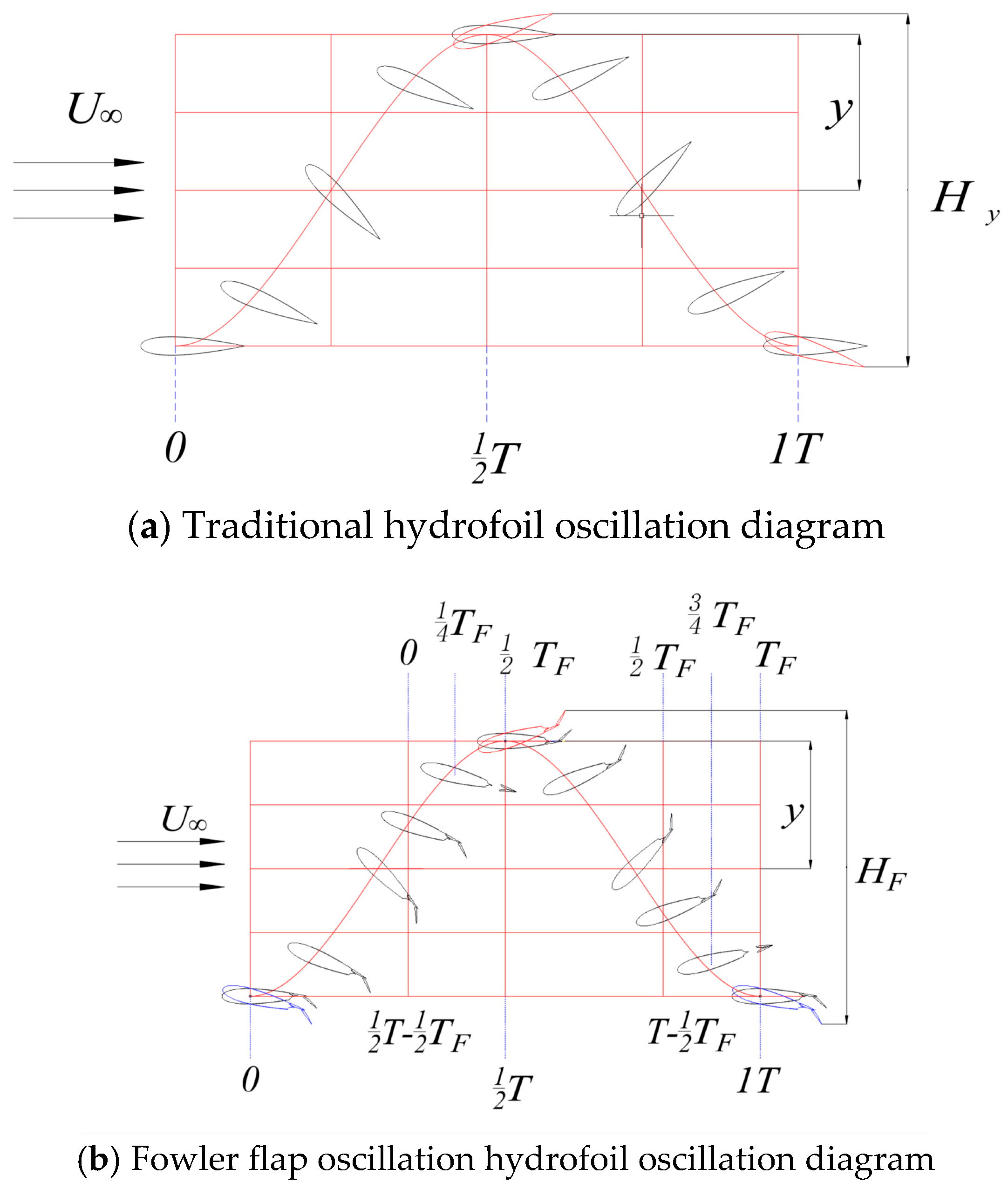
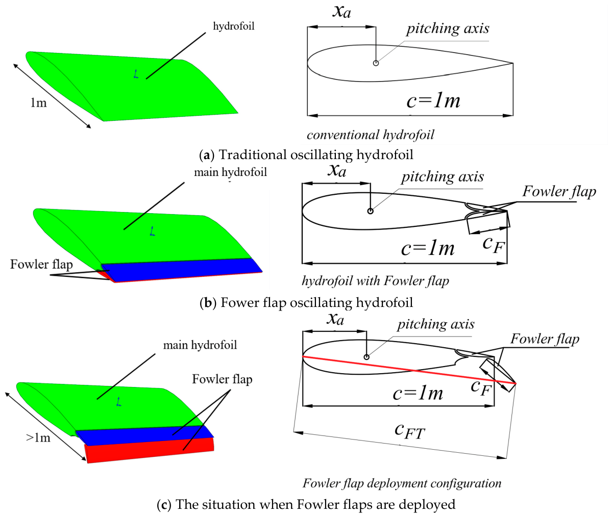
Fowler flaps are utilized in both aviation and maritime fields, and there is a considerable amount of research that has been conducted on them. In the fields of aeronautical engineering and ship rudders, trailing-edge flaps are often used to increase the lift of the overall hydrofoil. This paper studies two flap configurations explored in previous works. Research results suggest that flaps can improve the energy capture efficiency of oscillating hydrofoils [12,13]. The Fowler flap is also a commonly used flap structure, which has been widely considered in the application of increasing lift. Figure 1a shows the addition of double Fowler flaps to the trailing-edge portion of an oscillating hydrofoil.

The lift increment of the Fowler flap is greater than that of an ordinary single-slot flap, and its structure and motion mechanisms are simpler than those of double-slot or multi-slot flaps, which makes it more conducive to lift optimization. Its application in large civil aircraft is increasing. Tian [14] studied the aerodynamic characteristics of variable-arc Fowler flaps through numerical simulation and found that when the lift coefficient is greater than the critical value, the arc is conducive to improving the lift-to-drag ratio; the critical value is different under different conditions. The take-off and landing configurations were optimized using a 30% chord length Fowler flap. Compared with the reference configuration, the maximum lift coefficient of the optimized take-off configuration increased by 6.6%, and the stall angle and lift-to-drag ratio increased by 1.3° and 7.58%, respectively. Similar results were obtained on the wing/fuselage combination in general aviation aircraft. DeSalvo [15,16] used active aerodynamic flow control to improve the lift of the hydrofoil. The hydrofoil adopts the structure of a Fowler flap and a simple flap. This is achieved by driving the longitudinally arranged fluid-oscillating jets upstream and downstream of the leading edge of the flap. These jets increased the flow adhesion range along the flap surface when the flap deflection was up to 60°. The actuation significantly improved the performance of the Fowler-flap model (lift coefficient increased by 30%) compared to the optimized baseline configuration, and the high lift performance of the simple single-unit flap without crossflow gaps reached or exceeded that of the optimized baseline Fowler configuration. Steinbuch [17] introduced the design of a double-slotted Fowler flap for high-speed aerobatic aircraft. The maximum lift of the target was tested in a low-speed wind tunnel. The designed Fowler flap improved the maximum lift coefficient of the cross-section by about 0.4 higher than the value known from the literature. Kozlov [18] introduced the design process of a Fowler flap with adaptive elements. During takeoff and landing, shape memory alloy (SMA) actuators were used to influence and improve the gap geometry between the wing and the deployed flap, thereby improving the aerodynamic efficiency of the flap. In Yang’s [19] experiment, particle image velocimetry (PIV) technology was used to visualize the flow on the upper surface of the flap. The PIV results showed that flow separation on the flaps was completely suppressed by the same DBD actuators used in the simulation. Van Dam [20] believed that double-slotted Fowler flaps played a crucial role in the design of aircraft lift enhancement. David Demeier [21] detailed an experimental study that explored the effects of variations in flap inter-wing clearance and overlap size on the wake flow field of an airfoil equipped with trailing-edge Fowler flaps. When the angle of attack increased to near-stall conditions, it was found that increasing the flap inter-wing clearance could excite and improve the flow in the trailing-edge region of the main wing, while increasing the flap inter-wing overlap further promoted flow separation on the suction surface of the main wing, which could lead to a stall. Ernesto Benigni [22] proposed a multi-objective, multi-point optimization problem involving multi-element hydrofoils for high-lift devices. Pareto-optimal solutions were finally proposed, and the reasons for the performance improvement were discussed.

Drawing from the research on Fower flaps in the aviation and maritime fields, this article posits that flaps must exhibit specific motion patterns to ensure the practical operation of oscillating hydrofoils. Based on reference [11], this study proposes and further investigates the geometric parameters of the Fowler flap to enhance the lift and energy extraction capabilities of an oscillating hydrofoil. This research delves into the relationship between the energy extraction efficiency of an oscillating hydrofoil and its geometric and motion parameters, systematically evaluates the impact of dual Fowler flaps on the hydrodynamics and flow structure around the hydrofoil, and quantifies the energy extraction enhancement effect introduced by the Fowler flaps.

2. Numerical Modeling and Validation

2.1. Motion Model of Oscillating Hydrofoil

In the author’s previous research [11], a movable double Fowler flap was proposed for mounting on a hydrofoil generator. Figure 1a shows the hydrofoil structure without the Fowler flap, while Figure 1b shows the hydrofoil structure with the Fowler flap. Figure 1c shows the state when the Fowler flap is opened. The double Fowler flaps move separately according to the moving direction of the main wing structure, and make the flaps and the main wing adopt a certain camber. This design ensures that the Fowler flap is always in the most advantageous configuration to generate high lift and a high energy harvesting coefficient for the system.

The oscillating hydrofoil motion model is defined as the hydrofoil simultaneously experiencing a sinusoidal harmonic heaving motion y(t) and a pitching motion θ(t) under oncoming flows. Figure 1 depicts the geometric and kinematic parameters of a traditional hydrofoil and oscillating hydrofoil with Fowler flaps. In the literature [11], the Fowler flaps are divided into two parts, meaning there are two Fowler flaps. Each Fowler flap performs a Fowler motion during the heave motion. Therefore, the Fowler oscillating hydrofoil is divided into three parts. The first part is defined as the main hydrofoil, while the second and third parts are defined as the Fowler trailing-edge flaps with subscript F.

The c_F is the Fowler flap length; the periodic motion of a flapping wing energy harvester can be simplified as the combined periodic motions of heaving y(t) and pitching θ(t), as shown in Figure 2. The heave–pitch oscillating wing motion can be described formally as

$$y(t)=-y_0\sin (2\mathsf{\pi }ft+\phi )$$

(1)

$$\theta (t)=-{\theta }_{0}sin(2\mathsf{\pi }ft)$$

(2)

where φ is the phase difference between the heaving and pitching motions (φ is kept constant at 90° in this study). In order to unify the calculation, a dimensionless parameter f* is introduced. The reduced frequency f* is defined as $f^{\ast }=fc/U_{\infty }$, and the heaving velocity is $V_y=dy(t)/dt$. The minus sign in the formula means that the starting point of the hydrofoil movement is the lowest point. The same is true for pitch amplitude. Figure 2 shows the motion of a traditional hydrofoil without flaps, while Figure 2b shows the motion form of a Fowler-flap oscillating hydrofoil, with the positions of the Fowler flap displayed at various instants throughout the motion.

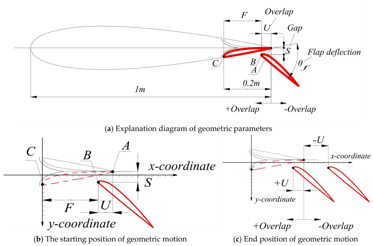
In Figure 3, point A is the rear-end point of the integral hydrofoil, point B is the front-end point of the flap (in open position), and point C is the front-end point of the flap (in closed position).

In order to define the movement of the Fowler flap, this paper introduces the following parameters:

• F, backward movement amount: The backward movement distance of the flap relative to the main wing, represented by Equation (3).
• U, the amount of overlap: The overlap distance between the retreating flap and the non-swing flap, represented by Equation (4). U has positive and negative values, and the 0 point has been marked in Figure 3. +U represents the overlap in the x-direction between the backward flap and the non-oscillating wing. −U represents that there is no longer any overlap between the retraction flap and the non-swinging flap, and the larger the U, the farther the retraction flap is from the non-swinging flap.
• S, vertical movement amount: The vertical distance between the retracted Fowler flap and the non-swing flap, represented by Equation (5);
• θ_F, swing angle: The swing angle of the Fowler flap. (In this article, θ_F is fixed at 40°).

For ease of description, this article defines three variables, F, U, and S. The defining equations are as follows:

$$F=\left|x_C-x_B\right|$$

(3)

$$U=x_B-x_A$$

(4)

$$S=\left|y_A-y_B\right|$$

(5)

In

Table 1. Location diagram of F, U, and S values of Fowler flaps.

F, U, S	Fowler Flap Deployment Position Diagram
F = 80 (U = −120) S = 0
F = 80 (U = −120) S = 30
F = 200 (U = 0) S = 0
F = 80 (U = 0) S = 50
F = 280 (U = 40) S = 0
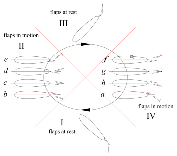
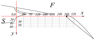
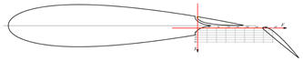
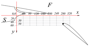
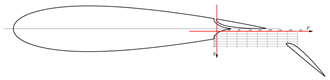
F = 280 (U = 80) S = 50

, several numerical values of F, U, and S parameters and their corresponding flap positions are listed. The annotations in the figure provide an intuitive understanding of the meaning of F, U, S values. Figure 4 shows the motion mode of a Fowler flap. The complete movement of each cycle can be divided into six phases. The specific forms of motion have been elaborated in previous studies [11].

2.2. Kinematic Calculation Equation and Numerical Methodology

The effective angle of attack has a positive relation to the pitching angle. The effective angle of attack is expressed as the combination of the plunging-induced and pitching angles [23], which can be expressed as follows:

$$V_{eff}\left(t\right)=\sqrt{U_{\infty }^2+V_y{\left(t\right)}^2}$$

(6)

$${\alpha }_{eff}=\arctan \left(V_y\left(t\right)/U_{\infty }\right)+\theta \left(t\right)$$

(7)

For most oscillating foils in hydrodynamic applications, the pitching axis is located at 1/3 chord length from the leading edge [24,25]. The corresponding force coefficients C_X, C_Y and moment coefficient C_M are defined as follows:

$$C_X(t)=F_x(t)/{\displaystyle \frac{1}{2}}\rho {U_{\infty }}^{2}c$$

(8)

$$C_Y(t)=F_y(t)/{\displaystyle \frac{1}{2}}\rho {U_{\infty }}^{2}c$$

(9)

$$C_M(t)=M_z(t)/{\displaystyle \frac{1}{2}}\rho {U_{\infty }}^2{c}^2$$

(10)

where F_x, F_y and M_z denote, respectively, the lift force, drag force, and pitching moment on the foil, and ρ the fluid density. The instantaneous power extraction P(t) and the time-averaged power $\overline{P}$ can be expressed as follows:

$$P(t)=P_L(t)+P_M(t)=F_Y(t){\displaystyle \frac{dy(t)}{dt}}+M(t){\displaystyle \frac{d\theta (t)}{dt}}$$

(11)

$$\overline{P}={\overline{P}}_L+{\overline{P}}_M={\displaystyle \frac{1}{T}}{\displaystyle {\displaystyle \underset{0}{\overset{T}{\int }}}P(t)dt}={\displaystyle \frac{1}{T}}{\displaystyle {\displaystyle \underset{0}{\overset{T}{\int }}}{P}_L(t)dt}+{\displaystyle \frac{1}{T}}{\displaystyle {\displaystyle \underset{0}{\overset{T}{\int }}}{P}_M(t)dt}$$

(12)

where P_L(t) is the instantaneous lift power extraction, P_M(t) is the instantaneous moment power extraction, ${\overline{P}}_L$ is the time-averaged lift power, and ${\overline{P}}_M$ is the time-averaged moment power. Furthermore, the non-dimensional instantaneous power coefficient C_p(t) and the cycle-averaged power coefficient ${\overline{C}}_p$ are denoted by

$$C_P(t)=P(t)/{\displaystyle \frac{1}{2}}\rho U_{\infty }^{3}c$$

(13)

$${\overline{C}}_P={\displaystyle \frac{1}{T}}{\displaystyle {\displaystyle \underset{0}{\overset{T}{\int }}}{C}_P(t)dt}=\overline{P}/{\displaystyle \frac{1}{2}}\rho U_{\infty }^{3}c$$

(14)

For a 2D hydrofoil, the swept area S of the oscillating foil equals the overall vertical extent of the foil motion. Therefore, the energy harvesting efficiency η can be defined as

$$\eta =\overline{P}/{\displaystyle \frac{1}{2}}\rho U_{\infty }^{3}S={\overline{C}}_P{\displaystyle \frac{c}{H}}$$

(15)

$${\eta }_g=\overline{P}/{\displaystyle \frac{1}{2}}\rho U_{\infty }^{3}S={\overline{C}}_P{\displaystyle \frac{c}{H_g}}$$

(16)

C_P is an instantaneous power value, C_X represents the magnitude of drag, C_Y represents the magnitude of lift, and η represents the ratio of obtained power to energy harvesting area. It can be understood as the amount of power that can be obtained within a certain energy harvesting flow field. The larger the η, the stronger the ability to obtain energy.

The calculation of sweep height has been explained in detail in article [11]. Figure 5 shows the comparison of sweep height between a conventional hydrofoil and Fowler-flap hydrofoil. It can be seen intuitively from Figure 5 that the sweeping height of the Fowler-flap hydrofoil is higher than that of the conventional hydrofoil. H is the sweep height of the conventional oscillating hydrofoil, and H_F is the sweep height of the oscillating hydrofoil with Fowler flaps. The equation is as follows:

$$H=\max \left\{\begin{array}{c}-2y\sin (2\mathsf{\pi }ft+\phi )+2TE\sin [-\theta \sin (2\mathsf{\pi }ft)]\\ -2y\sin (2\mathsf{\pi }ft+\phi )-2LE\sin [-\theta \sin (2\mathsf{\pi }ft)]\end{array}\right.$$

(17)

$$H_F=\max \left\{\begin{array}{c}\begin{array}{l}\left|-2y\sin (2\mathsf{\pi }ft+\phi )+2(T{E}_m-(c_F-F))\sin [-{\theta }_m\sin (2\mathsf{\pi }ft)])+2c_F\cos ([-{\theta }_m\sin (2\mathsf{\pi }ft)]-{\theta }_F)+2S\cos {\theta }_m(t)\right|\\ \left|-2y\sin (2\mathsf{\pi }ft+\phi )+2(T{E}_m-F)\sin [-{\theta }_m\sin (2\mathsf{\pi }ft)])+2c_F\cos ([-{\theta }_m\sin (2\mathsf{\pi }ft)]-{\theta }_F)+2S\cos {\theta }_m(t)\right|\end{array}\\ -2y\sin (2\mathsf{\pi }ft+\phi )-2L{E}_m\sin [-{\theta }_m\sin (2\mathsf{\pi }ft)]\end{array}\right.$$

(18)

2.3. Numerical Methodology

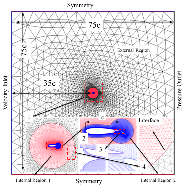
For a two-dimensional (2D) model, Theodorsen developed a closed-form solution of the hydrodynamic lift and moment on a thin plate undergoing harmonic oscillation motion in a uniform flow [26]. It has been widely used in the study of unsteady foil dynamics and flow-induced instability. The governing equations were discretized based on the finite volume method (FVM) using the software Fluent [26,27]. Figure 4 presents the information related to the boundary conditions and size of the computational region [28,29]. The far field boundary is set at a distance of 35c from the foil so that its effect on the flow surrounding the moving surface is negligible [26,30,31,32]. Triangle cells are used for meshing, except for the boundary layer which employs quadrilateral cells. The internal circular computational region includes two parts: internal region 1 and internal region 2. The internal circular computational region 1 experiences a synchronous heaving/pitching rigid movement with the foil. It assures no changes in the core computational region when internal region 2 is moving. Internal region 2 is a high-density region. The square fluid computational field is divided into four sections by sliding interfaces in the grid model. The centers of the three regions are located in the pitching axis (c/3) of the hydrofoil. The external region in the figure is a static area. During the movement of the internal region, the external region will be redrawn. Internal regions 1 and 2 are both moving areas, but the difference between internal region 1 and 2 is that internal region 1 is only moved as a whole grid, and its inner grid is not re-meshed, while the grid of internal region 2 is moving due to the internal movement of the hydrofoil, and the mesh must be re-meshed. This model uses interface sliding grid technology, which ensures that internal region 1 does not need to be re-meshed, and thus the amount of re-meshing of the external grid is greatly reduced.

The Reynolds number (Re) based on the far-stream velocity (U_∞) and the chord length (c) is Re = 2 × 10⁶. The previous study demonstrated that the time-averaged performance indicators are affected slightly by the choice of turbulence [33].

The one-equation Spalart–Allmaras turbulence model which requires a lower quality of mesh and in turn reduces computation time was chosen for our simulation [34,35,36]. The Pressure Implicit with Splitting of Operator (PISO) model is used for pressure–velocity coupling. Discretization based on the second-order upwind bound is selected for convection and diffusion terms. The first-order implicit method is employed for transient formulation. The absolute convergence criteria of the continuity and velocity components are set as 10⁻⁵. The hydrofoil’s movement is controlled through a User-Defined Function (UDF). In the actual simulation process, the value of y-plus near the hydrofoil is less than 5, which meets the requirements of the enhanced wall function processing method adopted by the Spalart–Allmaras model. The eighth period is selected as the starting point for the computing power coefficient and force coefficients because of the stable convergence computations.

2.4. Validation of Computation

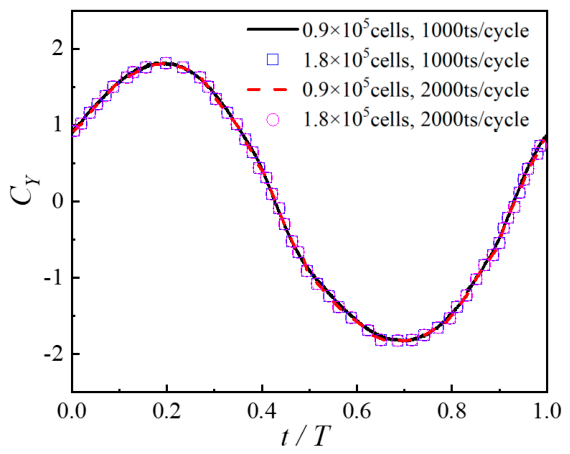
To verify the reliability of the mesh model, the grid number and time step independence were validated at different levels. Computational details and results are plotted in Figure 5. It can be seen that these plots with different mesh sizes and time steps overlap with each other; therefore, the effect of mesh size and time step quantity can be reasonably ignored. To reduce computation time without sacrificing accuracy, a number of cells—0.90 × 10⁵ (700 nodes on the foil)—and a time resolution of 1000 time steps per cycle were chosen in this study.

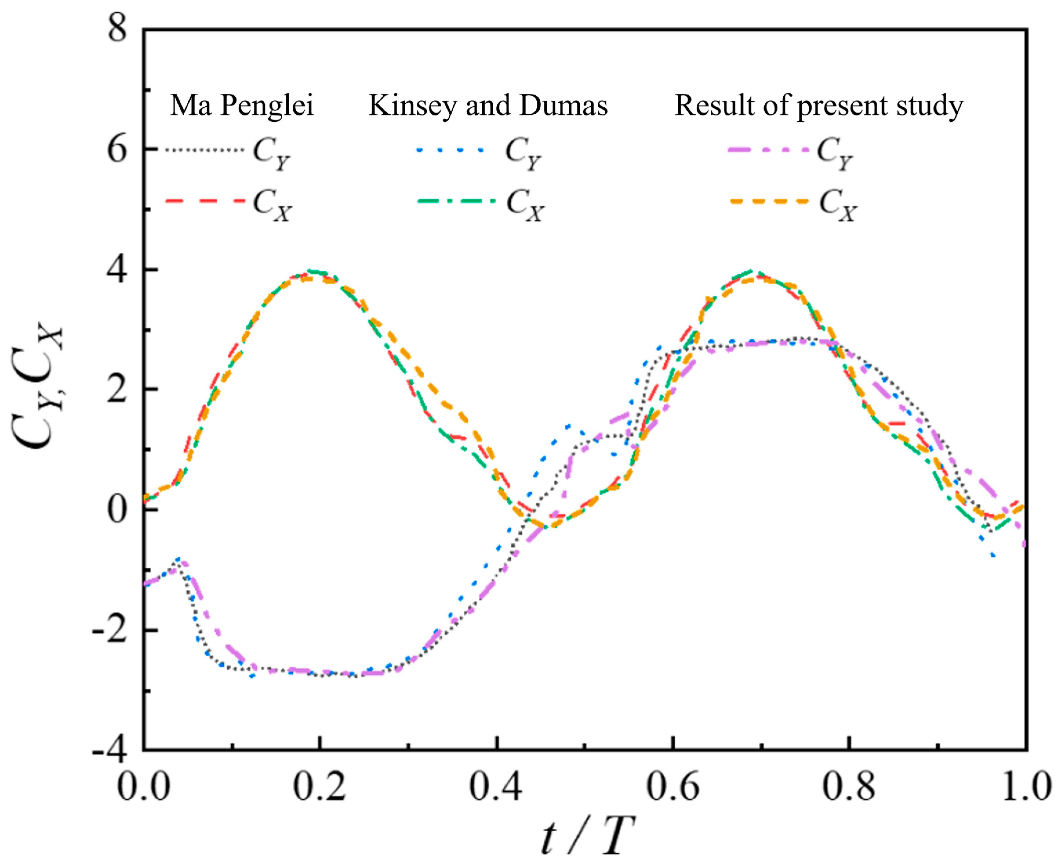
Kinsey and Dumas carried out the simulation of an oscillating hydrofoil [35,36] and studied the influence of hydrodynamic coefficients and geometric parameters. Their study can serve as touchstone for our model. The results of simulations of both models under the same conditions are presented in Figure 6 [36] (U_∞ =2 m/s, Reynolds number Re = 2 × 10⁶, Spalart–Allmaras turbulence model, θ = 75°, f* = 0.14, y₀ = c). Figure 7 indicates that the results of the present research are very close to those of Kinsey [36] and Ma [37], which demonstrates the validity of the numerical method.

3. Results and Discussions

All simulations in this study were applied to an NACA0018 foil under equivalent conditions of Re = 2 × 10⁶, y/c = 1 m, c_F = 0.2 m, ρ = 1020 kg/m³, U_∞ = 2 m/s, θ₀ = 45°, and θ_F = 40°. The main variables in this study are the Fowler motion F and slot value S. Their effects on the observed energy harvesting performance are discussed.

3.1. Effect of F on Power Coefficient

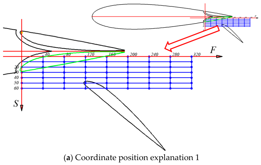
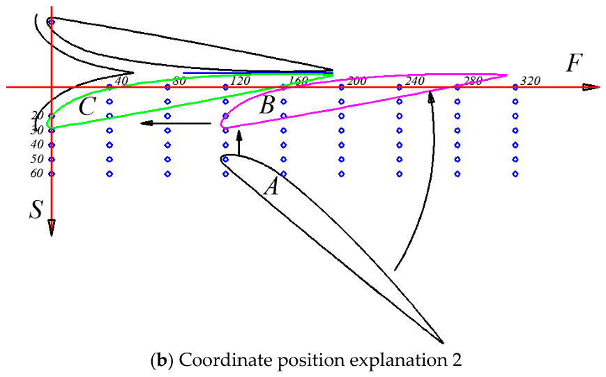
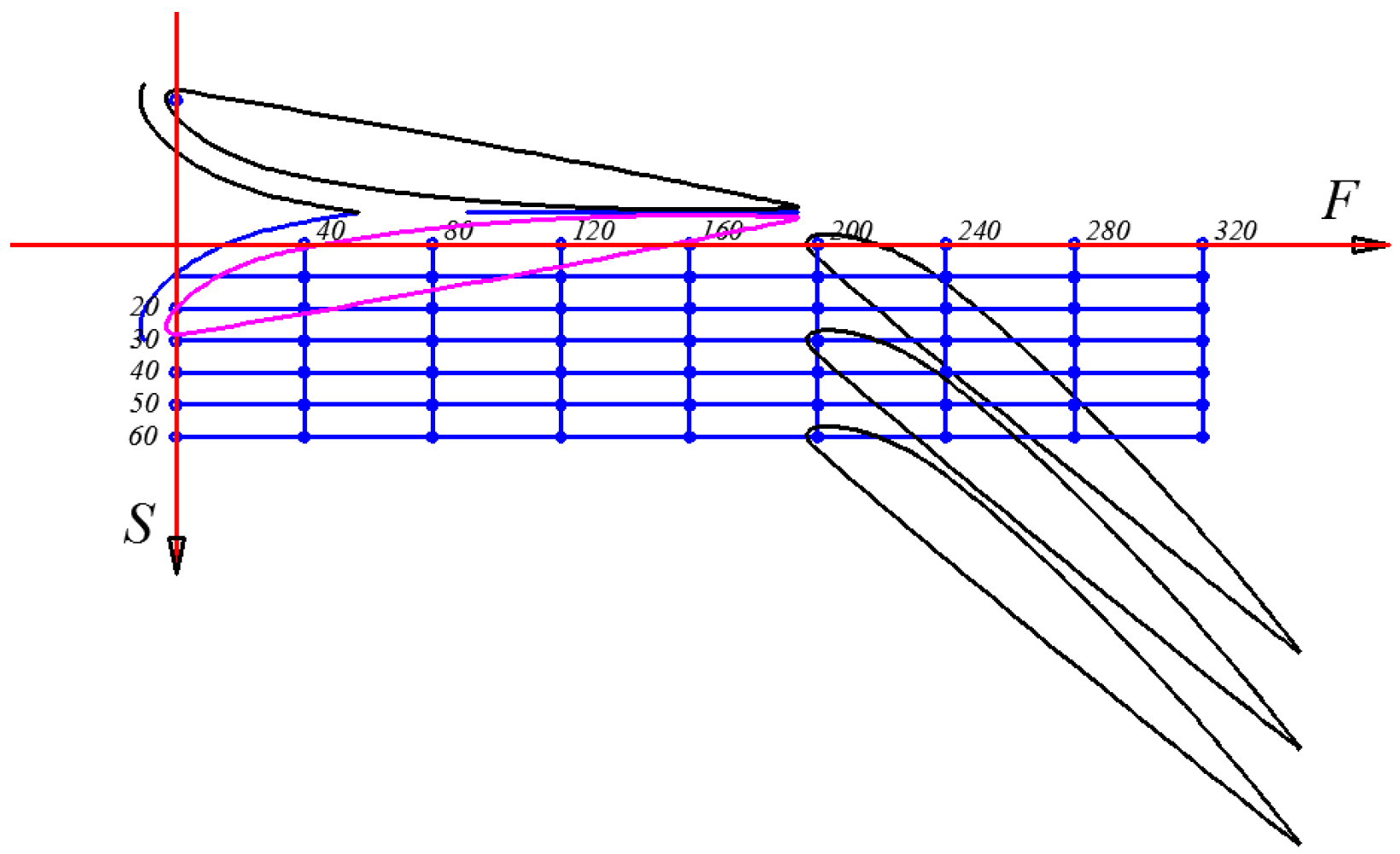
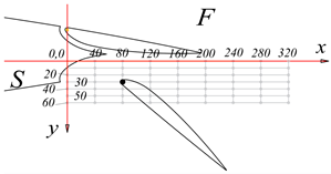
There are two variables in the coordinate system of Figure 6, Fowler motion F and seam value S. F is the horizontal movement of the Fowler flap relative to the main wing, and S is the vertical movement of the Fowler flap relative to the main wing. The magnitude of Fowler motion can affect the chord length c of the hydrofoil. An increase in chord length c can directly increase the lift of the hydrofoil. At the same time, due to the backward motion of the flap, the overall hydrofoil changes greatly compared with the original hydrofoil, and the hydrodynamic force and energy capture efficiency also change greatly. The size of the slot value s can affect the flow-field structure of the hydrofoil. When water flows through the slot, it will affect the forces on the main wing and flap. Therefore, these two parameters are important research variables.

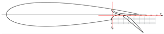
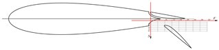
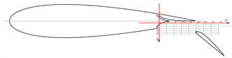
The motion of the Fowler flap is complex; in order to express the motion equation of Fowler flap intuitively, deployment and retraction position diagrams of Fowler flap are presented. The small blue circle in Figure 8b represents the rotation axis of the Fowler flap. When the Fowler flap is extended to the target position, the coordinates of the rotation axis are also marked in the coordinate system. For example, the coordinates (F = 120, S = 50) in Figure 8 represent the relative rotation axis of the Fowler flap, and the target deployment position is located in this coordinate. This coordinate system is used to calibrate Fowler motion F and slot value S. The movement of the Fowler flap can be described by the positions of the coordinates. For example, Figure 8 shows that the expanded position of the flap is position A, the middle position is position B, and the retracted position of the Fowler flap is position C. At this time, the leading-edge rotation-axis position of the flap is (F = 120, S = 50). The motion process can be summarized as follows, combined with the definition of motion formula: The motion of the Fowler flap is divided into two time periods. The first time period is from position a to position B, including two motions: (1) swing—the flap rotates relative to the rotation axis; (2) vertical movement—the whole flap has vertical upward movement relative to the main wing. The second time period is from B to C. In this period, the position of the flap is the horizontal position of B relative to the main wing, which is the horizontal movement to position C. The above description is the movement process of Fowler flap opening. The closing motion process is just the opposite of the opening process. We converted the coordinate values in Figure 8 into F, S, and U via Formulas (3)–(5). See Table 1 for specific values. In order to better illustrate Figure 8, this article has compiled

Table 2. F, S, and U calculated from Figure 8.

Chord, c, mm	F in Figure 8, mm	Fowler Motion, F	Overlap, U	S in Figure 8, mm	Gap, S
1000	0	0%	−20%	20	2%
1000	40	4%	−16%	30	3%
1000	80	8%	−12%	40	4%
1000	120	12%	−8%	50	5%
1000	160	16%	−4%	60	6%
1000	200	20%	0%
1000	240	24%	4%
1000	280	28%	8%
1000	320	32%	12%

, from which the coordinates of each point can be clearly seen.

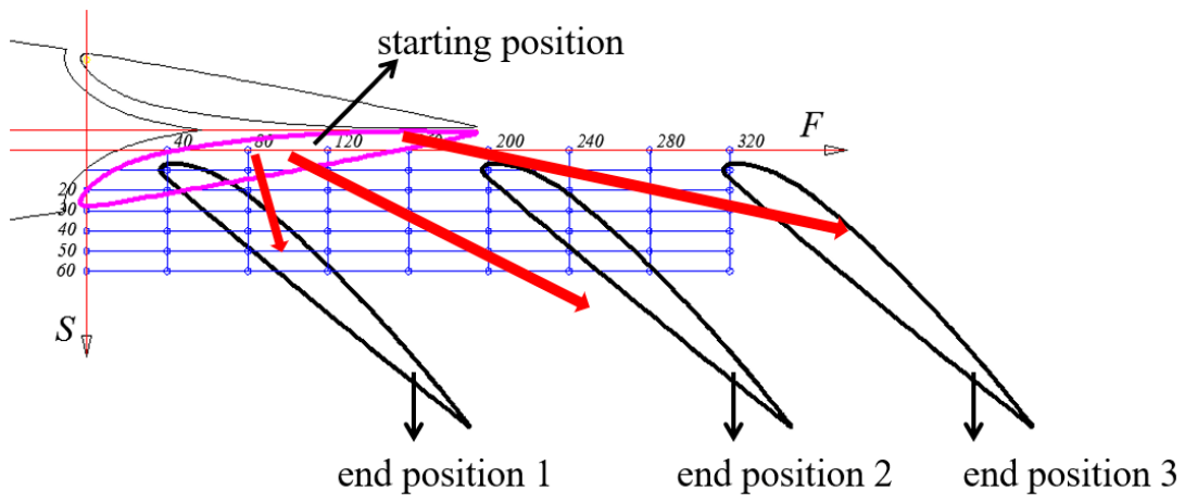
The position shown in Figure 9 is the end position of Fowler-flap movement. Under each fixed S value, the F value is increased to obtain different end positions. The value range of S is 0~60. Under each value of S, the value of F gradually increases, ranging from 0~320. The increase in F value indicates that the final motion position of the Fowler flap is farther away from the main wing, but the slot value s with the main wing remains unchanged.

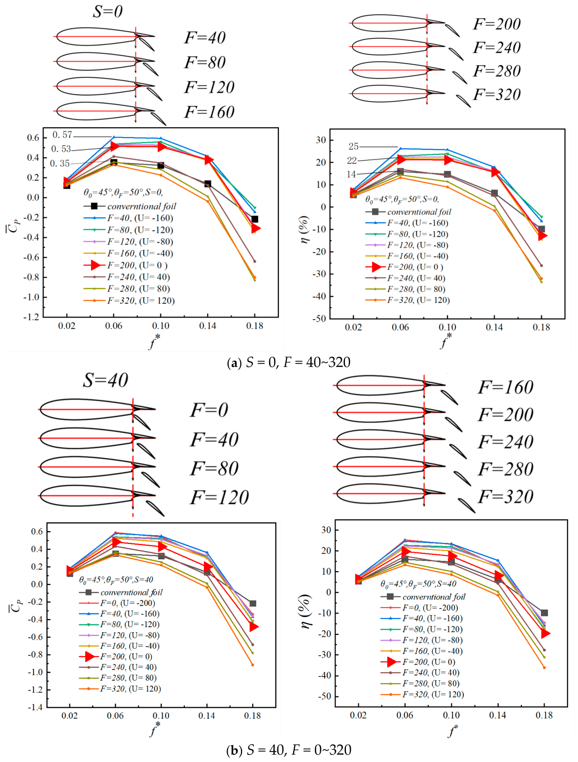
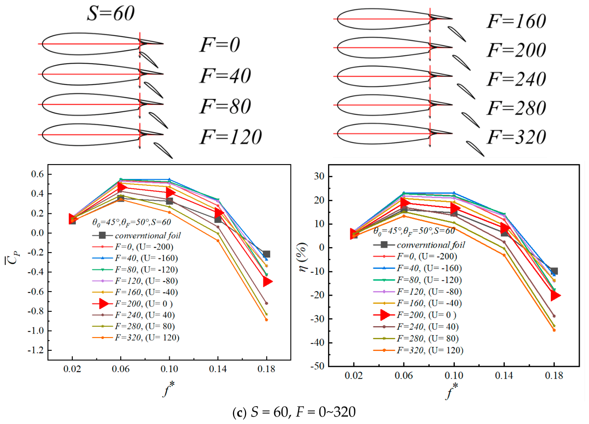
This section contains a comparative study on the changes in different Fowler motion F values under the condition of fixed S. All Fowler-flap motion forms are simulated according to the changes in different F and S coordinates of flap rotation axis O shown in Figure 10. In Figure 10a, when S = 0, the power curves at F = 40~200 are clustered together. It can be seen that the power change is not very obvious. It can be considered that when S = 0, the change in F value in the range of 40~200 has little effect on power and power coefficient. When F > 200, the brown circle line (F = 240) in Figure 10 suddenly drops and separates. At this time, the power with F ≥ 240 decreases significantly, and the greater the F value, the lower the power. It can be considered that when S = 0 and F ≥ 200, the greater the Fowler motion F, the smaller the power. In Figure 10b, when S = 40, the power curve of the red triangle (F = 200, U = 0%) also shows downward separation. By observing the other graph in Figure 10c, it can be seen that the clustering degree of the power curve with F = 40~200 is relatively sparse, and the power curve decreases significantly at this time. When s = 60, the value of F in the range of 40~200 will also have a great impact on the power coefficient. It can be seen from the summary that the power coefficient of the oscillating hydrofoil also decreases greatly after F > 200. The maximum ${\overline{C}}_P$ of the Fowler flap in Figure 10 is 57%, which is 59% higher than that of a conventional foil.

Referring to formulas in reference [11], the sweep height corresponding to the change in all Fowler motion and slot motion under the condition of Fowler flap length C_F = 0.2c is calculated. The energy capture efficiency can be calculated according to the formula, as shown in Figure 10. The average power shown in Figure 10 is very similar to the energy capture efficiency diagram, and the change trend is basically the same. It can be seen that the impacts of F and S value on the average power ${\overline{C}}_P$ and energy capture efficiency η are synchronous.

3.2. Effect of S on Power Coefficient

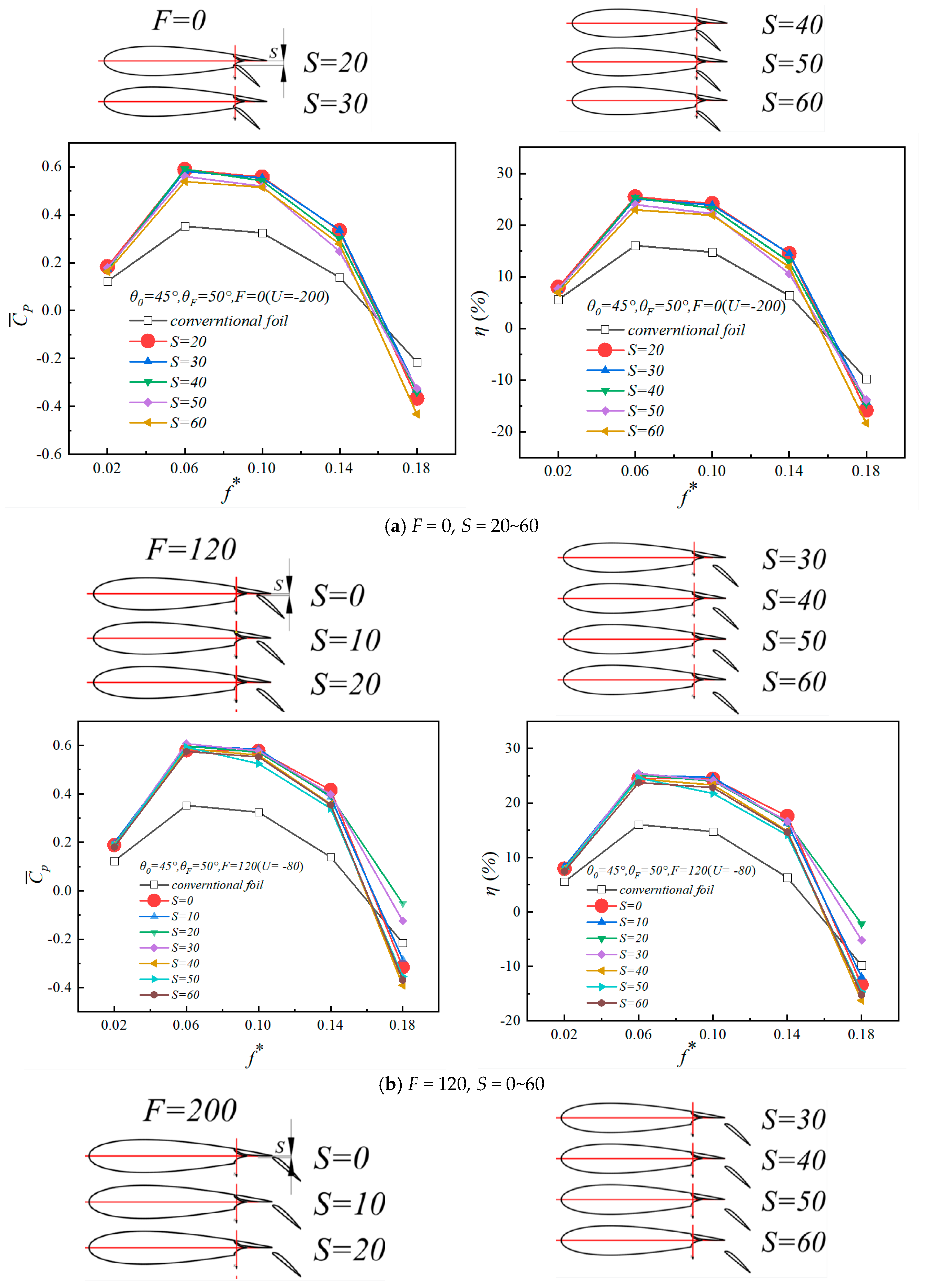
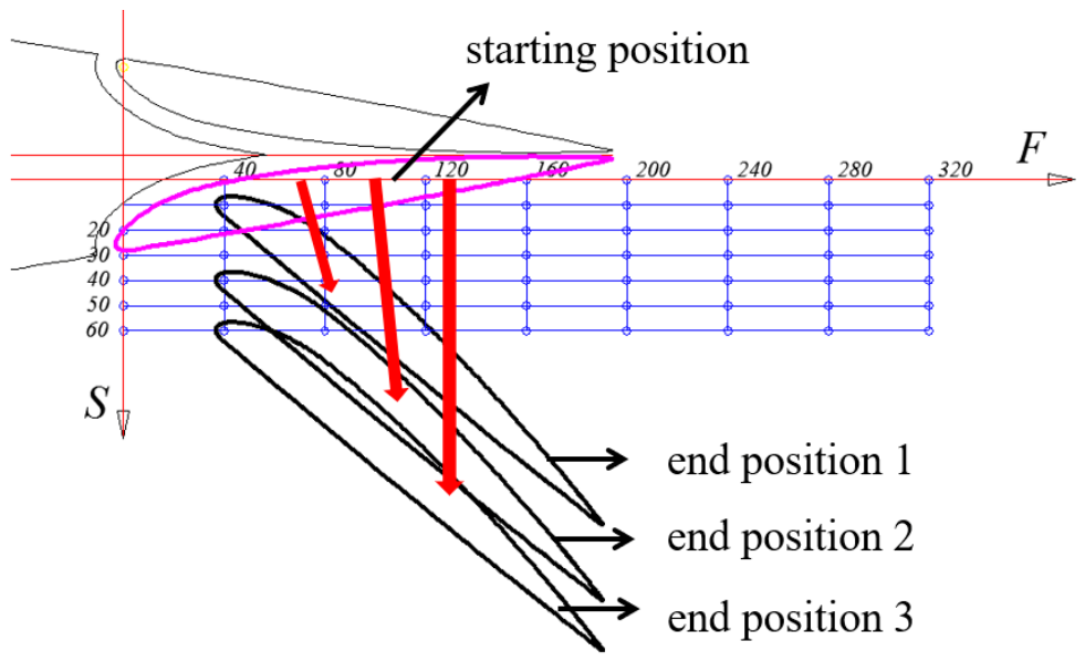
For better comparative analysis, the following Figure 11 fixes Fowler movement F and gradually increases the seam value S. The specific positions are shown in Figure 11.

The position shown in Figure 11 is the end position of Fowler-flap movement. Under each fixed F value, we increase the S value to obtain different end positions. The value of F is 0~320, and the value range of S is 0~60 under each F value. The greater the S value, the farther away the end position of the flap from the main wing in the Y-direction.

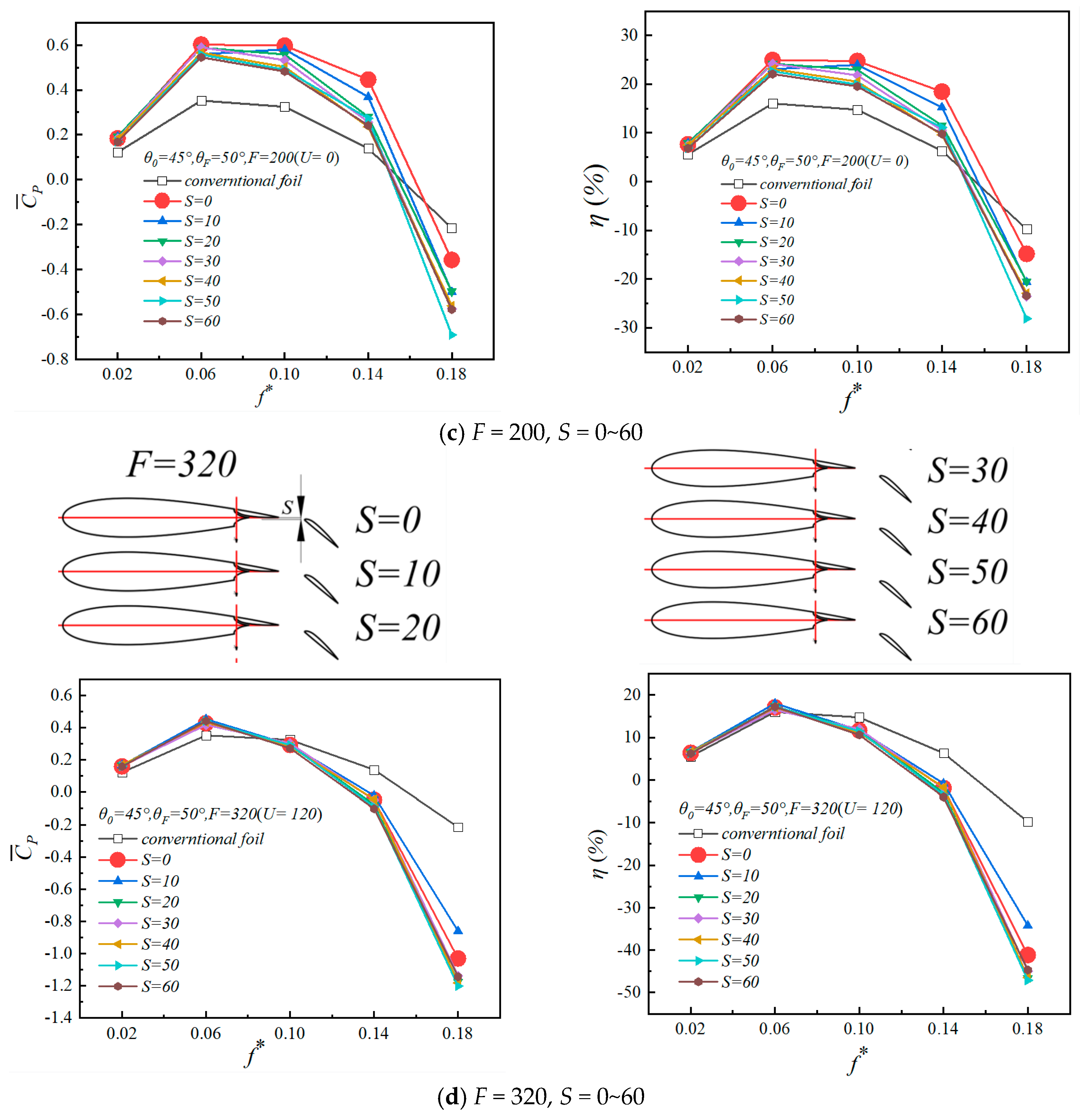
Figure 12 arranges the ${\overline{C}}_P$ change curves corresponding to different S values under the condition of keeping F unchanged. S value is the vertical position movement of the Fowler flap. It can be seen that when F = 0, with an increase in s value, the corresponding ${\overline{C}}_P$ at each oscillation frequency f* decreases, but the degree is not obvious. When F = 40, after the S value increases, the corresponding ${\overline{C}}_P$ decreases and begins to increase. When F = 200, the influence of s value on ${\overline{C}}_P$ is very obvious. At this time, the s value increases, and the power curve ${\overline{C}}_P$ in Figure 12c decreases to a great extent. At this time, the power curve distribution is sparse, and the influence of S value on power is very significant under this condition. When F > 200, the influence of S value starts to decrease again. When F = 320, the power curves almost coincide, but the power still decreases with the increase in S value. When F = 320, the maximum power coefficient in Figure 12d is only 45%, and when the frequency exceeds f* = 0.10, the power of the hydrofoil is less than that of a conventional hydrofoil.

To sum up, it can be seen that F = 200(U = 0%) is a characteristic position, which is shown in Figure 13. The figure shows the change in s from 0 to 60 under the condition of F = 200 and U = 0%.

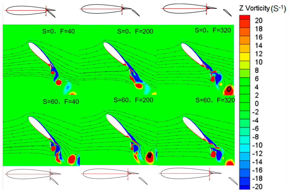
Figure 14 shows vorticity and streamline diagrams under different F and S values. It can be seen that the increase in F and S values will increase the distance between the main wing and the flap. After the gap increases, water can pass through the gap. If a large amount of water flows around the back of the hydrofoil through the gap, the differential pressure between the upper and lower hydrofoil will be reduced, and then the lift of the hydrofoil will be reduced. When the distance increases, more vortices will be generated after the flap, which are not conducive to energy collection. Z represents the vortex intensity, with the unit of S⁻¹. It can be simply understood as representing the kinetic energy of vortices in the fluid, but vortex intensity has a direction, with red representing clockwise and blue representing counterclockwise.

Summarizing the above results, when the trailing-edge flap is at F = 200(U = 0%), the leading edge of the flap and the trailing edge of the main wing are just at the critical point of contact, and the S value has a great influence on the change in power. The larger the S value, the smaller the power coefficient. When F < 200, S value has little effect on power. When the s value remains unchanged and S = 0, the Fowler flap overlaps with the main wing in the range of F < 200, and the power changes little. When F > 200, the Fowler flap and the main wing no longer overlap, and the slit value s increases rapidly. The increase in the slit value makes the vortex generated by the flap flow out of the slit, and the overall lift of the hydrofoil also begins to decrease, which directly leads to a decrease in power. A Fowler flap is a backward-slotted flap. According to the aviation design, the backward motion and slot value should improve the lift of the overall hydrofoil, but the motion form of an oscillating hydrofoil is different from that of flight. The motion angle of attack of an oscillating hydrofoil is very large, exceeding the stall angle of a conventional hydrofoil. When the main wing has stalled, the role of flaps is relatively weak, Therefore, it can be observed that the slot value s in the oscillating hydrofoil does not increase the lift, but an excessive slot value leads to a decrease in the lift coefficient.

3.3. Influence of F and S on Hydrodynamic Coefficient

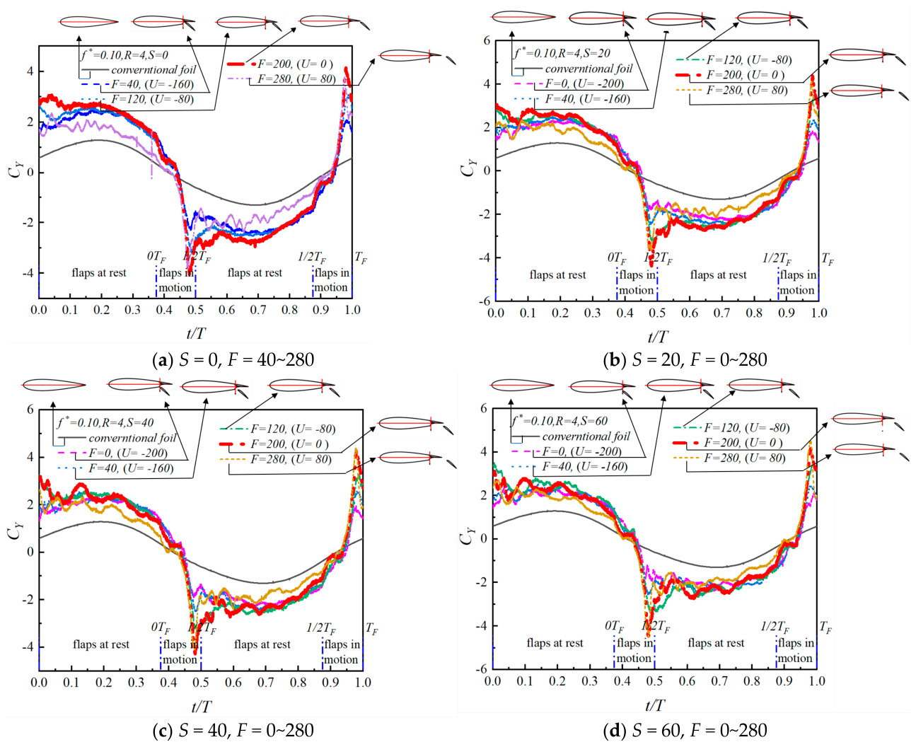
Figure 15 shows the change in lift coefficient in a cycle. Under the same S value, when the change range of F value is 0~200, C_Y changes little. After F > 200, although the chord length of the overall hydrofoil continues to increase, the horizontal distance between the flap and the main wing becomes larger, which makes the fluid between the trailing-edge flap and the main wing pass through the hydrofoil. The front pressure generated by the flap makes the fluid flow away from the slot and reduces the pressure on the lower surface of the hydrofoil. The lift of the integral hydrofoil must also be reduced. When F = 200(U = 0%), the horizontal distance between the main wing and the flap is the smallest, and the chord length of the hydrofoil is the largest, so the overall C_Y curve is the largest, as shown in the F = 200(U = 0%) curve in Figure 15.

Table 3. Comparison of average lift coefficient ${\overline{C}}_Y$.

${\overline{\mathit{C}}}_{\mathit{Y}}$	Conventional Foil		S = 0, F = 40	S = 0, F = 120	S = 0, F = 200	S = 0, F = 280
	0.5		0.821	1.815	2.165	1.95
		S = 20, F = 0	S = 20, F = 40	S = 20, F = 120	S = 20, F = 200	S = 20, F = 280
		1.693	1.826	2.004	2.078	1.568
		S = 40, F = 0	S = 40, F = 40	S = 40, F = 120	S = 40, F = 200	S = 40, F = 280
		1.698	1.782	1.979	1.959	1.573
		S = 60, F = 0	S = 60, F = 40	S = 60, F = 120	S = 60, F = 200	S = 60, F = 280
		1.670	1.809	2.019	1.925	1.643

compares the average lift coefficients ${\overline{C}}_Y$ under corresponding conditions, and it can be seen from the table that all hydrofoils equipped with Fowler flaps have higher lift coefficients than traditional hydrofoils. Under the conditions of S = 0 and F = 200, the overall streamline of the hydrofoil is the best, and the lift coefficient is also the highest. From the table, it can be concluded that the better the flow linearity of the hydrofoil, the greater the chord length of the hydrofoil, and the higher the lift coefficient. This is consistent with the conventional properties of airfoils.

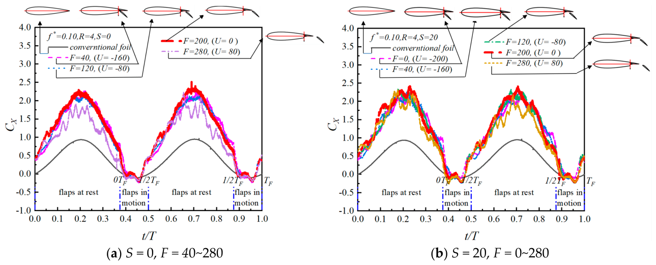
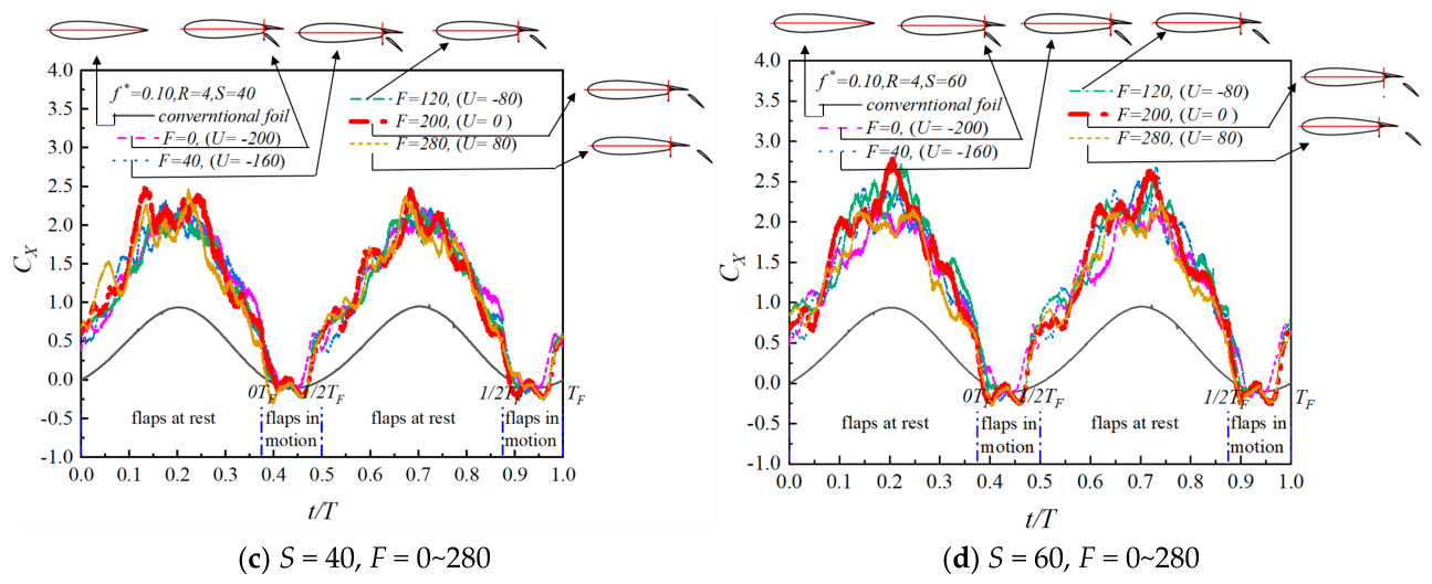
As can be seen from Figure 16, the overall drag of the Fowler-flap hydrofoil is larger than that of the traditional hydrofoil. The largest Fowler-flap drag coefficient is 1.16, while the drag coefficient of the traditional hydrofoil is 0.39, an increase in drag of three times. The trend is basically the same as that of the lift curve. In all the value ranges of F and S, the drag curve under the conditions of S = 0 and F = 200 is smooth and the fluctuation is the smallest. The average drag coefficient C_X (S = 0, F = 200) = 1.13. After f > 200, the drag begins to drop sharply, and the C_X (S = 0, F > 200) drag coefficient can be reduced to 0.90. The variation in drag coefficient is related to the overall shape of the hydrofoil, with smoother transitions resulting in a lower drag coefficient. Furthermore, an increase in the F value prevents the entire incoming flow from acting on the hydrofoil, leading to a reduction in drag but also a significant decrease in lift, which is detrimental to energy harvesting.

Table 4. Comparison of average drag coefficient ${\overline{C}}_X$.

${\overline{\mathit{C}}}_{\mathit{X}}$	Conventional Foil		S = 0, F = 40	S = 0, F = 120	S = 0, F = 200	S = 0, F = 280
	0.424		1.126	1.101	0.918	1.153
		S = 20, F = 0	S = 20, F = 40	S = 20, F = 120	S = 20, F = 200	S = 20, F = 280
		1.129	1.128	1.140	1.164	1.027
		S = 40, F = 0	S = 40, F = 40	S = 40, F = 120	S = 40, F = 200	S = 40, F = 280
		1.154	1.145306	1.123	1.161	1.125
		S = 60, F = 0	S = 60, F = 40	S = 60, F = 120	S = 60, F = 200	S = 60, F = 280
		1.161	1.264	1.302	1.260	1.130

compares the magnitude of the average drag coefficient under corresponding conditions. Compared to traditional hydrofoils, Fowler flaps increase lift while also increasing drag. Under all conditions of installing Fowler flaps, when S = 0 and F = 200, the overall streamline of the hydrofoil is the best and the drag coefficient is also the smallest. Based on the trend of lift coefficient variation, designing a streamlined shape is the optimal solution.

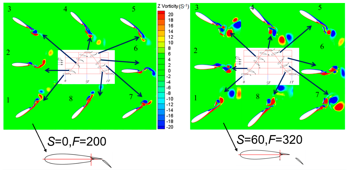
Figure 17 shows a comparison of vorticity under different geometric parameters. When S = 0 and F = 200, the overall hydrofoil curve formed by the Fowler flap and the main wing is smooth, and the vortices generated during the oscillation of the hydrofoil are relatively small. When S = 60, F = 320, the gap between the Fowler flap and the main wing becomes larger, which makes the overall streamlined shape of the hydrofoil less smooth. During operation, the hydrofoil experiences more fluctuations. As can be seen from the vorticity diagram, under these conditions, the wake vortices of the hydrofoil are stronger, more vortices are separated, and more energy is carried away, which is not collected by the hydrofoil. Therefore, we conclude that the overall streamlined shape of the hydrofoil is a very important influencing factor, as it ensures more stable force on the hydrofoil, thereby achieving better results in practical working environments. For the structure designed in this paper, when S = 0 and F = 200, both the energy capture efficiency and the force on the hydrofoil can achieve good results. Therefore, under these conditions, the overall performance of the hydrofoil is the best. The figure shows a comparison of vortices under two different geometric parameters. The vortex with S = 60 has a larger energy, which cannot be captured by the hydrofoil and can be understood as lost. Therefore, it can be seen from the maps that the higher the intensity of the hydrofoil’s vortex, the less energy it captures.

4. Conclusions

In the present research, a Fowler flap is proposed to improve the energy collection capacity of an oscillating hydrofoil, and we attempt to make the Fowler flap cooperate with the hydrofoil’s movement. Two-dimensional transient numerical simulation of oscillating hydrofoils—both a conventional foil and one with a Fowler flap—were carried out. The simulation results were analyzed comparatively with respect to the energy harvesting efficiency, and we included the effects of the Fowler movement F and slot value S. The results can be summarized as follows.

(1)

A Fowler-flap structure can increase the camber and chord length of the integral hydrofoil, and the movement of the Fowler flap is combined with the motion of the oscillating hydrofoil to increase the lift coefficient of the hydrofoil, thus increasing the energy collection efficiency of the oscillating hydrofoil. The maximum increase is 50%.

(2)

When Fowler motion has S = 0 and F = 200, the energy capture efficiency of the hydrofoil is the largest. At this time, the slot value S has a great influence on the change in power. The larger the S value, the smaller the power coefficient. The water will flow through the increased gap S, which is the direct reason for the reduction in the force on the hydrofoil. When F ≠ 200, the value of S will affect the power coefficient slightly.

(3)

The structure of the Fowler flap makes the overall hydrofoil smooth. When S = 0 and F = 200, the fluctuations in lift and drag of the oscillating hydrofoil are very small. The overall smoothness is similar to that of a conventional hydrofoil, but the lift and resistance are greatly improved.

This article has advantages in terms of its simulation results. The simulation results cannot guarantee the accuracy of experimental results, so it is necessary to conduct experimental research in subsequent work.

References

1. Kusiak, A.; Zhang, Z.; Verma, A. Prediction, operations, and condition monitoring in wind energy. Energy 2013, 60, 1–12. [Google Scholar] [CrossRef]
2. Balduzzi, F.; Drofelnik, J.; Bianchini, A.; Ferrara, G.; Ferrari, L.; Campobasso, M.S. Darrieus wind turbine blade unsteady aerodynamics: A three-dimensional Navier-Stokes CFD assessment. Energy 2017, 128, 550–563. [Google Scholar]
3. Khan, M.J.; Bhuyan, G.; Iqbal, M.T.; Quaicoe, J. Hydrokinetic energy conversion systems and assessment of horizontal and vertical axis turbines for river and tidal applications: A technology status review. Appl. Energy 2009, 86, 1823–1835. [Google Scholar] [CrossRef]
4. Lam, W.; Chen, L.; Hashim, R. Analytical wake model of tidal current turbine. Energy 2015, 79, 512–521. [Google Scholar] [CrossRef]
5. ORourke, F.; Boyle, F.; Reynolds, A. Tidal energy update 2009. Appl. Energy 2010, 87, 398–409. [Google Scholar] [CrossRef]
6. Uihlein, A.; Magagna, D. Wave and tidal current energy—A review of the current state of research beyond technology. Renew. Sustain. Energy Rev. 2016, 58, 1070–1081. [Google Scholar]
7. Neill, S.P.; Angeloudis, A.; Robins, P.E.; Walkington, I.; Ward, S.L.; Masters, I.; Lewis, M.J.; Piano, M.; Avdis, A.; Piggott, M.D.; et al. Tidal range energy resource and optimization—Past perspectives and future challenges. Renew. Energy 2018, 127, 763–778. [Google Scholar]
8. Zhang, D.; Ma, X.; Si, Y.; Huang, C.; Huang, B.; Li, W. Effect of Doubly Fed Induction GeneratorTidal Current Turbines on Stability of a Distribution Grid under Unbalanced Voltage Conditions. Energies 2017, 10, 212. [Google Scholar] [CrossRef]
9. Liu, Z.; Wang, Y.; Hua, X. Numerical studies and proposal of design equations on cylindrical oscillating wave surge converters under regular waves using SPH. Energy Convers. Manag. 2020, 203, 112242. [Google Scholar] [CrossRef]
10. Xu, J.; Sun, H.; Tan, S. Wake vortex interaction effects on energy extraction performance of tandem oscillating hydrofoils. J. Mech. Sci. Technol. 2016, 30, 4227–4237. [Google Scholar] [CrossRef]
11. Sun, G.; Wang, Y.; Xie, Y.; Ma, P.; Zhang, Y. Hydrodynamic and energy extraction properties of oscillating hydrofoils with a trailing edge flap. Appl. Ocean Res. 2021, 110, 102530. [Google Scholar] [CrossRef]
12. Sun, G.; Wang, Y.; Xie, Y.; Lv, K.; Sheng, R. Research on the effect of a movable gurney flap on energy extraction of oscillating hydrofoil. Energy 2021, 225, 120206. [Google Scholar] [CrossRef]
13. Sun, G.; Zhang, Q.; Sun, H.; Chi, M.; Liu, G. Hydrodynamic and energy extraction properties of oscillating hydrofoil with double Fowler flaps. Front. Mar. Sci. 2025, 12, 1651862. [Google Scholar] [CrossRef]
14. Tian, Y.; Wang, T.; Liu, P.; Feng, P. Aerodynamic/mechanism optimization of a variable camber Fowler flap for general aviation aircraft. Sci. China Technol. Sci. 2017, 60, 1144–1159. [Google Scholar]
15. DeSalvo, M.; Whalen, E.; Glezer, A. Enhancement of a fowler flap high-lift system using active flow control. In 52nd AIAA Aerospace Sciences Meeting—AIAA Science and Technology Forum and Exposition; SciTech: Seoul, Republic of Korea, 2014. [Google Scholar]
16. DeSalvo, M.; Whalen, E.; Glezer, A. High-Lift Performance Enhancement Using Active Flow Control. AIAA J. 2020, 58, 4228–4242. [Google Scholar] [CrossRef]
17. Steinbuch, M.; Marom, S.; Gabriel, E.; Koshorok, A. Aerodynamic design of double-slotted fowler flap for acrobatic aircraft Javelin. Res. Gate 2008, 2, 653–672. [Google Scholar]
18. Kozlov, O. Design and Modeling of the Fowler Flap with Adaptive Elements. In Proceedings of the ASME International Mechanical Engineering Congress and Exposition, Chicago, IL, USA, 5–20 November 2006. [Google Scholar]
19. Yang, L.; Li, J.; Cai, J.; Wang, G.; Zhang, Z. Lift Augmentation Based on Flap Deflection with Dielectric Barrier Discharge Plasma Flow Control over Multi-Element Airfoils. J. Fluids Eng. 2015, 138, 031401. [Google Scholar] [CrossRef]
20. Van Dam, C.P. The aerodynamic design of multi-element high-lift systems for transport airplanes. Prog. Aerosp. Sci. 2002, 38, 101–144. [Google Scholar]
21. Demel, D.; Ferchichi, M.; Allan, W.D.; Dghim, M. Two-dimensional experimental investigation on the effects of a fowler flap gap and overlap size on the wake flow field. J. Fluids Eng. 2017, 139, 021101. [Google Scholar]
22. Benini, E.; Ponza, R.; Massaro, A. High-lift multi-element airfoil shape and setting optimization using multi-objective evolutionary algorithms. J. Aircr. 2011, 48, 683–696. [Google Scholar]
23. Ma, P.; Yang, Z.; Wang, Y.; Liu, H.; Xie, Y. Energy extraction and hydrodynamic behavior analysis by an oscillating hydrofoil device. Renew. Energy 2017, 113, 648–659. [Google Scholar] [CrossRef]
24. Young, J.; Lai, J.C.; Platzer, M.F. A review of progress and challenges in flapping foil power generation. Prog. Aerosp. Sci. 2014, 67, 2–28. [Google Scholar] [CrossRef]
25. Chen, Z.; Jiao, B.; Sun, G.; Lin, H.; Sun, H. CFD analysis of the influence of structural parameters on the hydrodynamic characteristics of oscillating swept hydrofoils. Proc. Inst. Mech. Eng. Part M J. Eng. Marit. Environ. 2025, 240, 46–59. [Google Scholar] [CrossRef]
26. Theodorsen, T. General Theory of Aerodynamic Instability and the Mechanism of Flutter; NACA Technical Report; NASA: Washington, DC, USA, 1979. Available online: https://ntrs.nasa.gov/citations/19930090935 (accessed on 2 June 2026).
27. Xue, G.; Liu, Y.; Zhang, M.; Ding, H. Numerical analysis of hydrodynamics for bionic oscillating hydrofoil based on panel method. Appl. Bionics Biomech. 2016, 2016, 6909745. [Google Scholar] [CrossRef] [PubMed]
28. Gharali, K.; Johnson, D.A. Dynamic stall simulation of a pitching airfoil under unsteady freestream velocity. J. Fluids Struct. 2013, 42, 228–244. [Google Scholar] [CrossRef]
29. Amiralaei, M.R.; Alighanbari, H.; Hashemi, S.M. An investigation into the effects of unsteady parameters on the aerodynamics of a low Reynolds number pitching airfoil. J. Fluids Struct. 2010, 26, 979–993. [Google Scholar] [CrossRef]
30. Todorov, M. Aerodynamic characteristics of airfoil with single plain flap for light airplane wing. In Proceedings of the 2015 International Conference on Military Technologies (ICMT), Brno, Czech Republic, 20–21 May 2015; IEEE: New York, NY, USA, 2015. [Google Scholar]
31. Bos, F.M.; Lentink, D.; Van Oudheusden, B.W.; Bijl, H. Influence of wing kinematics on aerodynamic performance in hovering insect flight. J. Fluid Mech. 2008, 594, 341–368. [Google Scholar]
32. Lentink, D.; Gerritsma, M. Influence of airfoil shape on performance in insect flight. In Proceedings of the 33rd AIAA Fluid Dynamics Conference and Exhibit, Orlando, FL, USA, 23–26 June 2003. [Google Scholar]
33. Ashraf, M.A.; Young, J.; Lai, J.C.S.; Platzer, M.F. Numerical Analysis of an Oscillating-Wing Wind and Hydropower Generator. AIAA J. 2011, 49, 1374–1386. [Google Scholar] [CrossRef]
34. Kinsey, T.; Dumas, G.; Lalande, G.; Ruel, J.; Méhut, A.; Viarouge, P.; Lemay, J.; Jean, Y. Prototype testing of a hydrokinetic turbine based on oscillating hydrofoils. Renew. Energy 2011, 36, 1710–1718. [Google Scholar] [CrossRef]
35. Kinsey, T.; Dumas, G. Parametric study of an oscillating airfoil in a power-extraction regime. AIAA J. 2008, 46, 1318–1330. [Google Scholar] [CrossRef]
36. Kinsey, T.; Dumas, G. Computational fluid dynamics analysis of a hydrokinetic turbine based on oscillating hydrofoils. J. Fluids Eng. 2012, 134, 021104. [Google Scholar] [CrossRef]
37. Ma, P.; Wang, Y.; Xie, Y.; Han, J.; Sun, G.; Zhang, J. Effect of wake interaction on the response of two tandem oscillating hydrofoils. Energy Sci. Eng. 2019, 7, 431–442. [Google Scholar] [CrossRef]
Figure 1. Comparison between Fowler-flap oscillating hydrofoil and traditional oscillating hydrofoil.
Actuators 15 00367 g001
Figure 2. Periodic motion forms of oscillating hydrofoils with and without Fowler flaps.
Actuators 15 00367 g002
Figure 3. Geometric parameters of Fowler flap.
Actuators 15 00367 g003
Figure 4. Kinematic decomposition diagram of Fowler-flap oscillating hydrofoil.
Actuators 15 00367 g004
Figure 5. Grid detail and boundary conditions (NACA0018 foil; total cells: 0.9 × 10⁵; 700 nodes on the foil).
Actuators 15 00367 g005
Figure 6. Evolution of vertical force coefficient for different levels of cells and time steps at θ = 45°, cg = 3%c, f* = 0.10, y0 = c (ts indicates the time steps).
Actuators 15 00367 g006
Figure 7. Comparison of results between references [36,37] and present study for force coefficients CY and CX.
Actuators 15 00367 g007
Figure 8. Schematic diagrams of Fowler-flap movement.
Actuators 15 00367 g008aActuators 15 00367 g008b
Figure 9. Schematic diagram of fixed seam value S and gradually increasing F.
Actuators 15 00367 g009
Figure 10. Variation in curves of energy capture efficiency under different F and S conditions.
Actuators 15 00367 g010aActuators 15 00367 g010b
Figure 11. Schematic diagram of a fixed Fowler motion F and gradually increasing S.
Actuators 15 00367 g011
Figure 12. Variation in curves of energy capture efficiency under different S conditions with F constant.
Actuators 15 00367 g012aActuators 15 00367 g012b
Figure 13. Flap change position diagram at U = 0.
Actuators 15 00367 g013
Figure 14. Vorticity diagrams under different F and S values.
Actuators 15 00367 g014
Figure 15. One-cycle variation curves of lift coefficient under different F and S conditions.
Actuators 15 00367 g015
Figure 16. Variation in curves of drag coefficient in one cycle under different F and S conditions.
Actuators 15 00367 g016aActuators 15 00367 g016b
Figure 17. Vorticity contour maps corresponding to different geometric parameters.
Actuators 15 00367 g017