Fault-Tolerant Formation Control for Quadrotor UAVs with Disturbance Observer

Abstract

Underactuated and strongly coupled Quadrotor Unmanned Aerial Vehicle (QUAV) systems often face challenges in formation control due to actuator failures, external unknown disturbances, and limited communication resources. To address these issues, this paper proposes a periodic adaptive event-triggered fixed-time fault-tolerant control method based on a disturbance observer. First, a dynamic estimation and compensation scheme for actuator faults is developed by combining boundary layer theory with adaptive control techniques. Next, a fixed-time disturbance observer is designed to accurately estimate and compensate for external unknown disturbances. Furthermore, considering the communication burden imposed by real-time position updates, a Non-Monitoring Periodic Adaptive Event-Triggered Control (NM-PAETC) mechanism is proposed to reduce communication resource consumption, while ensuring that the formation system maintains the desired attitude angles under the influence of actuator faults and external disturbances. The proposed method enables fixed-time formation control under limited communication resources, and the system’s convergence time is independent of the initial state. Simulation results validate the effectiveness of the proposed method.

1. Introduction

In recent years, QUAVs have been increasingly deployed in applications such as military reconnaissance, environmental monitoring, disaster relief, and logistics owing to their flexible control, high-speed flight, and precise hovering capabilities [1]. However, the dynamic model of a QUAV is an underactuated, highly coupled nonlinear system, which presents substantial challenges in designing stable and robust control protocols for dynamically complex environments [2]. As the complexity of missions increases, the performance and task execution capabilities of a single UAV often prove insufficient for handling more intricate tasks. Consequently, multi-UAV formation control has emerged as a key research focus.

In multi-UAV formation control, the reliable operation of actuators is critical. However, as the operational time of QUAVs increases, actuator failures become inevitable, potentially leading to system instability or loss of control. Therefore, the development of fault-tolerant control strategies for multi-UAV systems is of paramount importance. Several studies have proposed various approaches to address these challenges [3,4,5,6,7,8]. For instance, Miao et al. proposed an efficient fault-tolerant control strategy for QUAV systems experiencing actuator failures [5]. Jiang et al. presented a compensation scheme for actuator faults in nonlinear MASs based on an adaptive gain mechanism [6]. Similarly, Zhao et al. introduced an adaptive fault-tolerant controller to mitigate actuator failures in QUAVs [7]. Additionally, Hua et al. applied boundary layer techniques to develop a fully distributed continuous fault-tolerant formation control protocol for compensating actuator failures [8]. It is noteworthy that during mission execution, multi-UAV formations must also contend with uncertainties, such as unknown external disturbances, which pose additional challenges to achieving formation stability and precise control.

To address the problem of external disturbances, researchers have proposed various control strategies, including observer techniques [9], neural networks [10], adaptive control [11], model predictive control [12], and robust control [11]. Among these, control methods based on observer techniques have gained increasing attention due to their advantages. They not only achieve asymptotic suppression of external disturbances but also provide more accurate responses to complex disturbances. To improve disturbance rejection in multi-UAV control systems, an adaptive finite-time disturbance observer was introduced [13]. A fixed-time disturbance observer was also proposed for QUAV systems to mitigate the compound disturbances affecting the system [14]. Additionally, Zhang et al. introduced an improved disturbance observer that not only estimates external disturbances but also enhances the system’s tracking performance and stability by incorporating disturbance estimation error parameters [15]. However, in practical applications, systems often face multiple constraints, such as unknown nonlinearities, time-varying actuator failures, and external disturbances, all of which adversely affect system performance. Addressing these issues can significantly increase the communication burden.

What needs to be emphasized is that implementing fixed-time formation control increases the communication cost for UAVs. Given the limited communication resources of individual UAVs, this constraint reduces the system’s ability to process information and avoid risks in complex environments. To conserve channel resources, event-triggered control (ETC) is often introduced to eliminate the need for continuous communication in closed-loop systems [16], and has been applied in UAVs [17,18], Unmanned Ground Vehicles (UGVs) [19], and other nonlinear systems [20,21]. While traditional event-triggered mechanisms have demonstrated significant potential in resource-constrained applications [22,23], their fixed-threshold triggering conditions are unable to flexibly adapt to real-time changes in system states, thus affecting control performance. To overcome this limitation, dynamic event-triggered mechanisms (DETC) have been proposed [24]. A dynamic event-triggered control algorithm has been introduced to achieve distributed formation control in UAVs with constrained communication resources [25]. These mechanisms dynamically adjust the triggering conditions based on system state variations by incorporating adaptive variables, thereby improving communication resource utilization.

On the other hand, QUAV formation control will require faster and more accurate position and attitude tracking in the future. Studies show that finite-time control improves the convergence time, accuracy, and disturbance rejection performance of multi-UAV formation systems [26]. In practical engineering applications, the demand for rapid stability is even more urgent. Furthermore, the applicability of control methods is often limited by the difficulty of obtaining initial states. To address these issues, researchers have begun to focus on fixed-time control to enhance the performance of multi-UAV formation systems [27,28]. Gong et al. presented a fixed-time controller designed for the attitude stabilization of QUAVs [29]. A fixed-time control strategy was applied to UAV formations, achieving fast convergence in the system [30]. The fixed-time control method not only met the system’s stability time requirements but also mitigated the impact of initial states on system stability.

In summary, this paper presents a fixed-time fault-tolerant control method based on a disturbance observer with periodic adaptive event-triggering, addressing the formation control problem of multi-UAV quadrotor systems. The proposed method takes into account actuator time-varying failures, unknown time-varying parameters, external unknown disturbances, and limited communication resources. The control strategy ensures that the system maintains formation structure and that the tracking error converges within a fixed time, even in the presence of these challenges. The main contributions of this paper are as follows:

• The method integrates boundary layer theory and adaptive control techniques to estimate and compensate for actuator faults, achieving formation control in fixed time, with the system’s convergence time independent of the initial state.
• The observer quickly estimates unknown disturbances, while the developed NM-PAETC mechanism reduces communication resource consumption, ensuring the system maintains the desired attitude angles during formation control.

The structure of the article is outlined below. Section 2 introduces the dynamics model of a QUAV, covering actuator failures, relevant definitions, and lemmas; Section 3 constructs a fixed-time observer and verifies the system stability; Section 4 presents a periodic event-triggered fixed-time fault-tolerant control method; Section 5 validates the feasibility of the control strategy through simulation experiments; finally, Section 6 summarizes the main findings of this study.

2. Problem Formulation

2.1. Dynamics Model of a QUAV

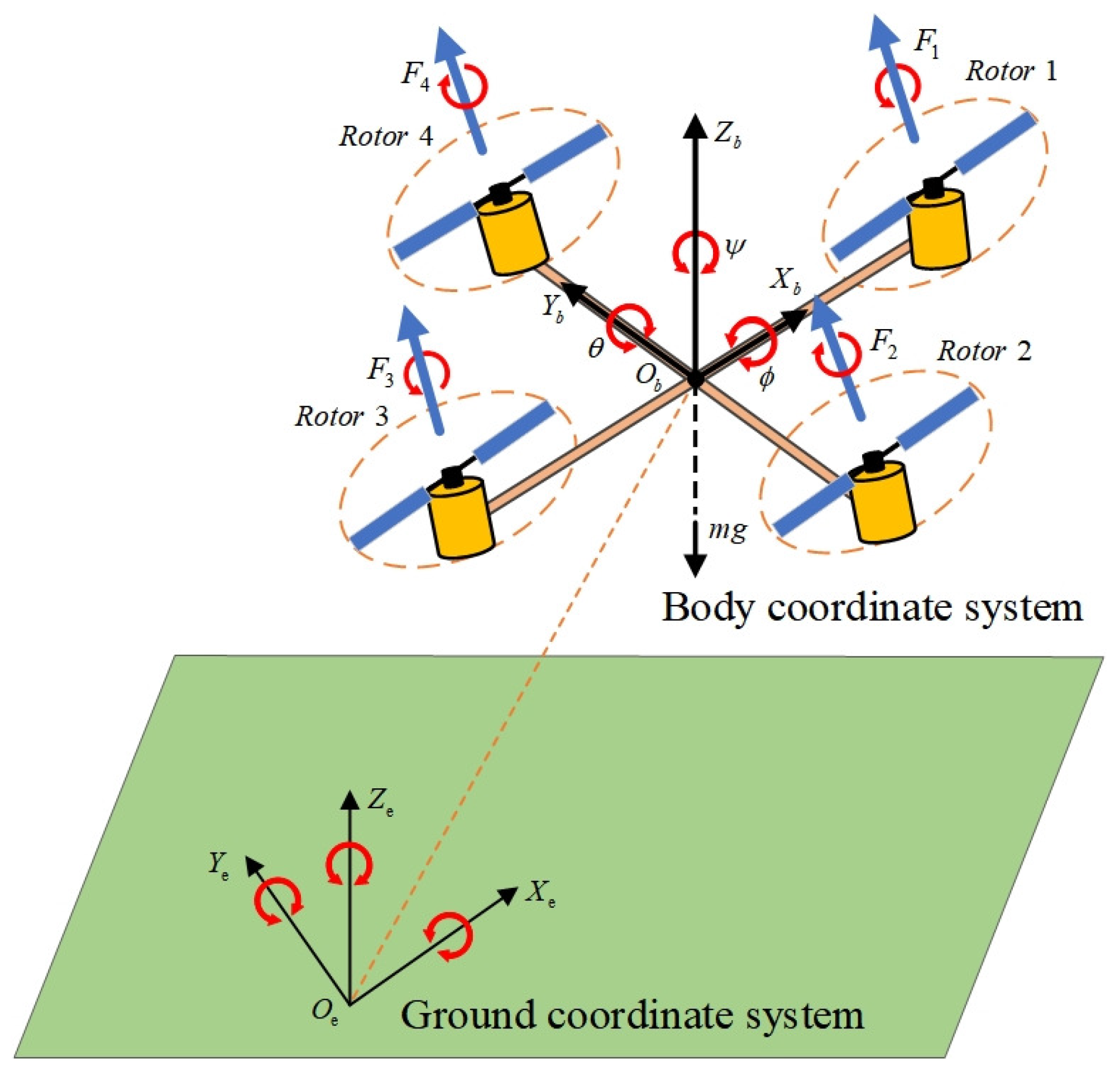
The center of mass of the UAV in the ground coordinate system is represented by $P_k={\left[x_k,y_k,z_k\right]}^T\in {\mathbb{R}}^3$. The UAV’s orientation is described by the Euler angles: roll ${\varphi }_k$, pitch ${\theta }_k$, and yaw ${\psi }_k$. The angular velocity vector in the ground frame is given by $\mathcal{A}={\left[{\dot{\varphi }}_k,{\dot{\theta }}_k,{\dot{\psi }}_k\right]}^T\in {\mathbb{R}}^3$. Figure 1 presents a multi-UAV system composed of a QUAV, with the notation and orientation definitions provided in

Table 1. The coordinate frame.

Notation	Orientation
$O_b$	Center of gravity of the QUAV
$O_b{X}_b$	The roll axis pointing in the forward direction of the QUAV
$O_b{Y}_b$	The pitch axis pointing to the left side of the QUAV
$O_b{Z}_b$	The yaw axis is perpendicular to $O_b{X}_b$ and points upward
$O_{\mathrm{e}}$	Initial position of the QUAV
$O_{\mathrm{e}}{X}_{\mathrm{e}}$	Pointing north and parallel to the Earth’s horizontal plane
$O_{\mathrm{e}}{Y}_{\mathrm{e}}$	Pointing in the true east direction and perpendicular to $O_{\mathrm{e}}{X}_{\mathrm{e}}$
$O_{\mathrm{e}}{Z}_{\mathrm{e}}$	Pointing upwards, perpendicular to to both $O_{\mathrm{e}}{X}_{\mathrm{e}}$ and $O_{\mathrm{e}}{Y}_{\mathrm{e}}$

.

The dynamic model of a QUAV with parameter uncertainties and external disturbances is considered [14,18]:

$$\begin{array}{cccc}\hfill & & \hfill \left\{\begin{array}{cc}& {\ddot{x}}_k={\displaystyle \frac{u_{k,1}}{m_k}}\left(cos{\varphi }_{k}sin{\theta }_{k}cos{\psi }_k+sin{\varphi }_{k}sin{\psi }_k\right)-{\displaystyle \frac{K_{k,1}}{m_k}}{\dot{x}}_k+{\displaystyle \frac{{\aleph }_{k,1}}{m_k}}\hfill \\ & {\ddot{y}}_k={\displaystyle \frac{u_{k,1}}{m_k}}\left(sin{\varphi }_{k}sin{\theta }_{k}cos{\psi }_k-cos{\varphi }_{k}sin{\psi }_k\right)-{\displaystyle \frac{K_{k,2}}{m_k}}{\dot{y}}_k+{\displaystyle \frac{{\aleph }_{k,2}}{m_k}}\hfill \\ & {\ddot{z}}_k={\displaystyle \frac{u_{k,1}}{m_k}}(cos{\varphi }_{k}cos{\theta }_k)-g-{\displaystyle \frac{K_{k,3}}{m_k}}{\dot{z}}_k+{\displaystyle \frac{{\aleph }_{k,3}}{m_k}}\hfill \\ & {\ddot{\varphi }}_k={\displaystyle \frac{u_{k,2}}{I_{k,z}}}+{\dot{\theta }}_k{\dot{\psi }}_k{\displaystyle \frac{I_{k,y}-I_{k,z}}{I_{k,x}}}+{\displaystyle \frac{{\varpi }_k{J}_{k,r}}{I_{k,x}}}{\dot{\theta }}_k-{\displaystyle \frac{K_{k,4}}{I_{k,x}}}{\dot{\varphi }}_k+{\displaystyle \frac{{\aleph }_{k,4}}{I_{k,x}}}\hfill \\ & {\ddot{\theta }}_k={\displaystyle \frac{u_{k,3}}{I_{k,z}}}+{\dot{\varphi }}_k{\dot{\psi }}_k{\displaystyle \frac{I_{k,z}-I_{k,x}}{I_{k,y}}}-{\displaystyle \frac{{\varpi }_k{J}_{k,r}}{I_{k,x}}}{\dot{\varphi }}_k-{\displaystyle \frac{K_{k,5}}{I_{k,y}}}{\dot{\theta }}_k+{\displaystyle \frac{{\aleph }_{k,5}}{I_{k,y}}}\hfill \\ & {\ddot{\psi }}_k={\displaystyle \frac{u_{k,4}}{I_{k,z}}}+{\dot{\varphi }}_k{\dot{\theta }}_k{\displaystyle \frac{I_{k,x}-I_{k,y}}{I_{k,z}}}-{\displaystyle \frac{K_{k,6}}{I_{k,z}}}{\dot{\psi }}_k+{\displaystyle \frac{{\aleph }_{k,6}}{I_{k,z}}}\hfill \end{array}\right.& \end{array}$$

(1)

where $m_k$ represents the mass of the UAV; unknown disturbances in the system are represented by ${\aleph }_{k,v}\left(v=1,2,\dots ,6\right)$; g represents the gravitational acceleration; $I_{k,x}$, $I_{k,y}$ and $I_{k,z}$ denote the moment of inertia of the body coordinate axes $O_b{X}_b$, $O_b{Y}_b$ and $O_b{Z}_b$, respectively; l represents the distance from the center of the rotor to the centroid; $J_{k,r}$ denotes the inertia moment of the rotor; ${\varpi }_k$ is overall residual rotor angular vector; $K_{k,\epsilon }\left(\epsilon =1,2,\dots ,6\right)$ represents the unknown aerodynamic coefficients of the kth UAV in the dynamics of position and attitude. Furthermore, the relationship between the control input $u_{k,i}$ and the rotor thrust $F_{k,i}$ is given by

$$\begin{array}{cccc}& & \hfill u_{k,1}=C_{k,t}\left({\omega }_{k,1}^2+{\omega }_{k,2}^2+{\omega }_{k,3}^2+{\omega }_{k,4}^2\right)={\sum }_{i=1}^4{F}_{k,i}& \end{array}$$

(2)

$$\begin{array}{cccc}& & \hfill u_{k,2}=C_{k,t}\left({\omega }_{k,2}^2-{\omega }_{k,4}^2\right)=F_{k,2}-F_{k,4}& \end{array}$$

(3)

$$\begin{array}{cccc}& & \hfill u_{k,3}=C_{k,t}\left({\omega }_{k,3}^2-{\omega }_{k,1}^2\right)=F_{k,3}-F_{k,1}& \end{array}$$

(4)

$$\begin{array}{cccc}& & \hfill u_{k,4}=C_{k,\alpha }\left({\omega }_{k,2}^2+{\omega }_{k,4}^2-{\omega }_{k,3}^2-{\omega }_{k,1}^2\right)& \end{array}$$

(5)

where $C_{k,t}$ represents the lift coefficient, the coefficient of rotor thrust acting in the yaw direction is represented by $C_{k,\alpha }$, ${\omega }_{k,i}$ represents the rotor speed, and $F_{k,i}$ is the lift generated by the rotor.

Assumption 1

([14]). The ground is considered a horizontal plane while neglecting the effect of Earth’s curvature, with the gravitational acceleration maintained at g.

Assumption 2

([31]). The QUAV possesses absolute symmetry, and the geometric center of the body remains constant; there exists a disturbance ${\aleph }_{k,v}\left(t\right)$ in the system that is continuous, differentiable, and bounded, such that $\left|{\aleph }_{k,v}\right|\le z_{k,v}$, where $z_{k,v}$ is a constant.

Assumption 3

([32]). The signals $x_d^i$, $y_d^i$, $z_d^i$, ${\psi }_d^i\in {\Delta }_{\infty },(i=0,1)$ of the virtual leader are known, continuous, and bounded, where $\left(i\right)$ denotes the ith derivative of the variable, and they possess at least second-order continuous derivatives.

2.2. Definition and Lemma

Lemma 1

([33]). Consider the system $\dot{x}=f\left(x\right)$, where $x\in {\mathbb{R}}^n$. If there exists a positive definite and continuous function $V\left(x\right)$ that satisfies the following condition:

$$\begin{array}{cccc}& & \hfill \dot{V}\left(x\right)\le -\Psi V^{q1}\left(x\right)-\Phi V^{q2}\left(x\right)+\Gamma & \end{array}$$

(6)

where $\Phi >0$, $\Psi >0$, $0<q_1<1$, $q_2>1$, and $\Gamma >0$ are constants, it can be deduced that the system $\dot{x}=f\left(x\right)$ exhibits practical fixed-time stability. The residual set of the solution is denoted by Θ, and the predefined convergence time by $T_m$.

$$\begin{array}{cccc}& & \hfill \Theta =\left\{x|V\left(x\right)\le min\left\{{\left({\displaystyle \frac{\epsilon }{\left(1-\lambda \right)\Psi }}\right)}^{{\displaystyle \frac{1}{q_1}}},{\left({\displaystyle \frac{\epsilon }{\left(1-\lambda \right)\Phi }}\right)}^{{\displaystyle \frac{1}{q_2}}}\right\}\right\}& \end{array}$$

(7)

$$\begin{array}{cccc}& & \hfill T_m\le {\displaystyle \frac{1}{\Psi \lambda \left(1-q_1\right)}}+{\displaystyle \frac{1}{\Phi \lambda \left(q_2-1\right)}}& \end{array}$$

(8)

where $0<\lambda <1$.

Lemma 2

([34]). For $\chi \in$ and $\delta >0$, one has

$$\begin{array}{cccc}& & \hfill 0\le \left|\chi \right|-\chi tan\mathrm{h}\left({\displaystyle \frac{\chi }{\delta }}\right)\le 0.2785\delta & \end{array}$$

(9)

Lemma 3

([35]). For ${\chi }_1\in$, ${\chi }_2\in$, ${\delta }_1>0$, ${\delta }_2>0$ and $k>0$, one has:

$$\begin{array}{cccc}& & \hfill \begin{array}{cc}& {\left|{\chi }_1\right|}^{{\delta }_1}{\left|{\chi }_2\right|}^{{\delta }_2}\le {\displaystyle \frac{{\delta }_1}{{\delta }_2+{\delta }_1}}k{\left|{\chi }_1\right|}^{{\delta }_1+{\delta }_2}+{\displaystyle \frac{{\delta }_2}{{\delta }_2+{\delta }_1}}{k}^{-{\displaystyle \frac{{\delta }_1}{{\delta }_2}}}{\left|{\chi }_2\right|}^{{\delta }_1+{\delta }_2}\hfill \end{array}& \end{array}$$

(10)

Lemma 4

([36]). Given that $k_i>0$ for $i=1,2,\cdots ,n$, $0<b_1<1$, and $1<b_2<\infty$, one has:

$$\begin{array}{cccc}& & \hfill {\left({\displaystyle \sum _{i=1}^n}{k}_i\right)}^{b_1}\le {\displaystyle \sum _{i=1}^n}{k}_i^{b_1}& \end{array}$$

(11)

$$\begin{array}{cccc}& & \hfill {\left({\displaystyle \sum _{i=1}^n}{k}_i\right)}^{b_2}\le {\displaystyle \frac{1}{n^{1-b_2}}}{\displaystyle \sum _{i=1}^n}{k}_i^{b_2}& \end{array}$$

(12)

Lemma 5

((Young’s inequality) [37]). For $\forall x_1\in \mathbb{R}$ and $\forall x_1\in \mathbb{R}$, one has:

$$\begin{array}{cccc}& & \hfill x_1{x}_2\le {\displaystyle \frac{{\kappa }^b}{b}}{\left|x_1\right|}^b+{\displaystyle \frac{1}{\mu {\kappa }^{\mu }}}{\left|x_2\right|}^{\mu }& \end{array}$$

(13)

where $b>1$, $\mu >1$, $\kappa >0$ and $\mu -1={\displaystyle \frac{1}{b-1}}$.

Lemma 6

([38]). For ${\chi }_3\in$ and any $b_4>0$, one has:

$$\begin{array}{cccc}& & \hfill 0\le \left|{\chi }_3\right|<b_4+{\displaystyle \frac{{\chi }_3^2}{\sqrt{{\chi }_3^2+{\kappa }_1^2}}}& \end{array}$$

(14)

2.3. Actuator Faults

In practical applications, the influence of external uncertainties or factors such as hardware aging and wear can lead to actuator failures in UAVs. These failures inevitably result in discrepancies between the actuator’s input and output, thereby affecting the system’s performance. Inspired by [39], actuator failures can be described using the following mathematical model:

$$\begin{array}{cccc}& & \hfill u_{k,v}\left(t\right)=h_{k,v}\left(t\right){\overline{u}}_{k,v}\left(t\right)+{ħ}_{k,v}\left(t\right),t\ge t_{k,v}^f& \end{array}$$

(15)

where ${\overline{u}}_{k,v}$ and $u_{k,v}$ represent the input and output of the actuator, respectively. $h_{k,v}\left(t\right)$ indicates the health factor, ${ħ}_{k,v}\left(t\right)$ represents the uncontrollable parameter portion of the control signal, $t_{k,v}^f$ denotes the moment when the actuator fails, and v denotes the number of actuators.

Assumption 4

([40]). In the actuator failure model, the continuous “health factor” $h_{k,v}\left(t\right)$ and the uncontrollable parameter ${ħ}_{k,v}\left(t\right)$ are time-varying, unknown but bounded, satisfying $0\le {\underline{h}}_{k,v}\le h_{k,v}\left(t\right)\le 1$ and $\left|{ħ}_{k,v}\right|\le {\overline{ħ}}_{k,v}<\infty$, ${\overline{ħ}}_{k,v}>0$.

3. Fixed-Time Disturbance Sliding-Mode Observer and Stability Analysis

During mission execution, UAVs may encounter unknown external disturbances such as wind speed variations and airflow turbulence, which can affect their flight trajectory and attitude. To accurately estimate and compensate for these disturbances, an observer was designed to provide estimates of the disturbances within a fixed time, enabling a rapid response.

For the position subsystem, taking the $x_k$ direction as an example, ${\tau }_{k,1,1}=x_k$ and ${\tau }_{k,1,2}={\dot{x}}_k$ are set to construct the corresponding second-order system model:

$$\begin{array}{cccc}\hfill & & \hfill \left\{\begin{array}{c}{\dot{\tau }}_{k,1,1}={\tau }_{k,1,2}\hfill \\ {\dot{\tau }}_{k,1,2}=F_{k,1}+d_{k,1}\hfill \end{array}\right.& \end{array}$$

(16)

where $F_{k,1}={\displaystyle \frac{u_{k,1}}{m_k}}\left(cos{\varphi }_{k}sin{\theta }_{k}cos{\psi }_k+sin{\varphi }_{k}sin{\psi }_k\right)={\displaystyle \frac{u_{k,1}}{m_k}}\left(A_k+S_k\right)$ is the known input-related nominal term, and $d_{k,1}=-{\displaystyle \frac{K_{k,1}}{m_k}}{\dot{x}}_k+{\displaystyle \frac{{\aleph }_{k,1}}{m_k}}$ is the unknown composite disturbance in the $x_k$ direction.

Assumption 5.

The composite disturbance $d_{k,v}\left(t\right)$ is continuous and bounded. That is, there exists an unknown positive constant ${\overline{d}}_{k,v}$ such that $|d_{k,v}\left(t\right)|\le {\overline{d}}_{k,v},k=1,2,\dots ,N,v=1,2,\dots ,6$.

Remark 1.

The composite disturbance $d_{k,v}\left(t\right)$ contains not only the external disturbance but also the uncertain damping term and the nonlinear coupling term in the corresponding channel. Therefore, the disturbance observer is designed to estimate $d_{k,v}\left(t\right)$, rather than only the external disturbance.

To achieve disturbance identification and estimation, the auxiliary variable is introduced as ${\phi }_{k,1}={\tau }_{k,1,2}-{\sigma }_{k,1}$.

The auxiliary dynamics are designed as

$${\dot{\sigma }}_{k,1}=F_{k,1}+{\lambda }_{k,1}{\upsilon }_{k,1}$$

(17)

where ${\lambda }_{k,1}$ is the observer gain, and ${\upsilon }_{k,1}$ is the discontinuous injection term. Since $d_{k,1}={\dot{\tau }}_{k,1,2}-F_{k,1}$, one obtains

$${\dot{\phi }}_{k,1}=d_{k,1}-{\lambda }_{k,1}{\upsilon }_{k,1}$$

(18)

The discontinuous injection term is designed as

$${\upsilon }_{k,1}={\kappa }_{k,1,1}{\phi }_{k,1}+{\kappa }_{k,1,2}\mathrm{Sgn}\left({\phi }_{k,1}\right)+{\kappa }_{k,1,3}{\mathrm{sig}}^{2q-1}\left({\phi }_{k,1}\right)+{\kappa }_{k,1,4}{\mathrm{sig}}^3\left({\phi }_{k,1}\right)$$

(19)

where ${\kappa }_{k,1,i}>0$, $(i=1,2,3,4)$, are observer design parameters. The operator ${\mathrm{sig}}^a(·)$ is defined as

$${\mathrm{sig}}^a\left(\phi \right)=|\phi {|}^a\mathrm{Sgn}\left(\phi \right)$$

(20)

where $\mathrm{Sgn}(·)$ denotes the Filippov set-valued sign function, i.e.,

$$\mathrm{Sgn}\left(·\right)=\left\{\begin{array}{cc}1,& ·>0\\ \left[-1,1\right],& ·=0\\ -1,& ·<0\end{array}\right.$$

(21)

The disturbance estimate is defined as the equivalent value of the discontinuous injection term:

$${\widehat{d}}_{k,1}={\lambda }_{k,1}{\upsilon }_{k,1}^{\mathrm{eq}}$$

(22)

where ${\widehat{d}}_{k,1}$ denotes the estimated value of $d_{k,1}$, and $0\le \left|d_{k,1}\right|\le {\overline{d}}_{k,1}$ holds.

Accordingly, the disturbance estimation error is defined as

$${\tilde{d}}_{k,1}=d_{k,1}-{\widehat{d}}_{k,1}$$

(23)

The fixed-time stability of the designed observer is demonstrated under the given assumptions by choosing the following Lyapunov function:

$$V_{k,1,d}={\displaystyle \frac{1}{2}}{\phi }_{k,1}^2$$

(24)

By differentiating $V_{k,1,d}$, one has

$$\begin{array}{cc}\hfill {\dot{V}}_{k,1,d}& ={\phi }_{k,1}{\dot{\phi }}_{k,1}={\phi }_{k,1}\left(d_{k,1}-{\lambda }_{k,1}{\upsilon }_{k,1}\right)\hfill \\ \hfill & =-{\lambda }_{k,1}{\kappa }_{k,1,1}{\phi }_{k,1}^2-{\lambda }_{k,1}{\kappa }_{k,1,2}\left|{\phi }_{k,1}\right|\hfill \\ \hfill & -{\lambda }_{k,1}{\kappa }_{k,1,3}|{\phi }_{k,1}{|}^{2q}-{\lambda }_{k,1}{\kappa }_{k,1,4}|{\phi }_{k,1}{|}^4+d_{k,1}{\phi }_{k,1}\hfill \end{array}$$

(25)

According to Assumption 5, one has $d_{k,1}{\phi }_{k,1}\le {\overline{d}}_{k,1}\left|{\phi }_{k,1}\right|$.

Therefore,

$$\begin{array}{cc}\hfill {\dot{V}}_{k,1,d}\le & -{\lambda }_{k,1}{\kappa }_{k,1,1}{\phi }_{k,1}^2-{\lambda }_{k,1}\left({\kappa }_{k,1,2}-{\overline{d}}_{k,1}\right)\left|{\phi }_{k,1}\right|\hfill \\ \hfill & -{\lambda }_{k,1}{\kappa }_{k,1,3}|{\phi }_{k,1}{|}^{2q}-{\lambda }_{k,1}{\kappa }_{k,1,4}|{\phi }_{k,1}{|}^4\hfill \end{array}$$

(26)

If the observer parameter satisfies ${\lambda }_{k,v}{\kappa }_{k,1,2}>{\overline{d}}_{k,1}$, then

$${\dot{V}}_{k,1,d}\le -{\lambda }_{k,1}{\kappa }_{k,1,3}|{\phi }_{k,1}{|}^{2q}-{\lambda }_{k,1}{\kappa }_{k,1,4}|{\phi }_{k,1}{|}^4$$

(27)

Since $|{\phi }_{k,1}{|}^{2q}=2^q{V}_{k,1,d}^q,|{\phi }_{k,1}{|}^4=4V_{k,1,d}^2$, one obtains

$${\dot{V}}_{k,1,d}\le -c_{k,1,1}{V}_{k,1,d}^q-c_{k,1,2}{V}_{k,1,d}^2$$

(28)

where $c_{k,1,1}=2^q{\lambda }_{k,1}{\kappa }_{k,1,3},c_{k,1,2}=2^2{\lambda }_{k,1}{\kappa }_{k,1,4}$.

According to Lemma 1, the auxiliary variable converges to zero within a fixed time. The settling time satisfies

$$T_{k,1,d}\le {\displaystyle \frac{1}{c_{k,1,1}(1-q)}}+{\displaystyle \frac{1}{c_{k,1,2}}}$$

(29)

As $t\ge T_{k,1,d}$, after the sliding manifold is reached, the sliding motion is maintained in the Filippov sense, namely, ${\phi }_{k,1}=0,{\dot{\phi }}_{k,1}=0$.

From ${\dot{\phi }}_{k,1}=d_{k,1}-{\lambda }_{k,1}{\upsilon }_{k,1}=0$, the equivalent injection term satisfies $d_{k,1}={\lambda }_{k,1}{\upsilon }_{k,1}^{\mathrm{eq}}$. Since the disturbance estimate is defined as ${\widehat{d}}_{k,1}={\lambda }_{k,1}{\upsilon }_{k,1}^{\mathrm{eq}}$, one obtains ${\widehat{d}}_{k,1}\to d_{k,1}$.Therefore, the disturbance estimation error satisfies

$${\tilde{d}}_{k,1}=d_{k,1}-{\widehat{d}}_{k,1}\to 0\left(t\ge T_{k,1,d}\right)$$

(30)

Thus, the proposed observer not only guarantees the fixed-time convergence of the auxiliary variable ${\phi }_{k,1}$ but also proves that the disturbance estimation error converges to zero after the observer settling time.

Similarly, the discontinuous injection terms for $y_k$, $z_k$, ${\varphi }_k$, ${\theta }_k$, and ${\psi }_k$ are designed as

$$\begin{array}{c}{\upsilon }_{k,2}={\kappa }_{k,2,1}{\phi }_{k,2}+{\kappa }_{k,2,2}\mathrm{Sgn}\left({\phi }_{k,2}\right)+{\kappa }_{k,2,3}{\mathrm{sig}}^{2q-1}\left({\phi }_{k,2}\right)+{\kappa }_{k,2,4}{\mathrm{sig}}^3\left({\phi }_{k,2}\right)\hfill \\ {\upsilon }_{k,3}={\kappa }_{k,3,1}{\phi }_{k,3}+{\kappa }_{k,3,2}\mathrm{Sgn}\left({\phi }_{k,3}\right)+{\kappa }_{k,3,3}{\mathrm{sig}}^{2q-1}\left({\phi }_{k,3}\right)+{\kappa }_{k,3,4}{\mathrm{sig}}^3\left({\phi }_{k,3}\right)\hfill \\ {\upsilon }_{k,4}={\kappa }_{k,4,1}{\phi }_{k,4}+{\kappa }_{k,4,2}\mathrm{Sgn}\left({\phi }_{k,4}\right)+{\kappa }_{k,4,3}{\mathrm{sig}}^{2q-1}\left({\phi }_{k,4}\right)+{\kappa }_{k,4,4}{\mathrm{sig}}^3\left({\phi }_{k,4}\right)\hfill \\ {\upsilon }_{k,5}={\kappa }_{k,5,1}{\phi }_{k,5}+{\kappa }_{k,5,2}\mathrm{Sgn}\left({\phi }_{k,5}\right)+{\kappa }_{k,5,3}{\mathrm{sig}}^{2q-1}\left({\phi }_{k,5}\right)+{\kappa }_{k,5,4}{\mathrm{sig}}^3\left({\phi }_{k,5}\right)\hfill \\ {\upsilon }_{k,6}={\kappa }_{k,6,1}{\phi }_{k,6}+{\kappa }_{k,6,2}\mathrm{Sgn}\left({\phi }_{k,6}\right)+{\kappa }_{k,6,3}{\mathrm{sig}}^{2q-1}\left({\phi }_{k,6}\right)+{\kappa }_{k,6,4}{\mathrm{sig}}^3\left({\phi }_{k,6}\right)\hfill \end{array}$$

(31)

where ${\kappa }_{k,v,1},{\kappa }_{k,v,2},{\kappa }_{k,v,3},{\kappa }_{k,v,4}$ are positive-definite parameters of the injection items, and ${\lambda }_{k,v}{\kappa }_{k,v,2}>{\overline{d}}_{k,v}$ holds.

Consequently, the proposed fixed-time disturbance observer can reconstruct the unknown composite disturbances within a fixed time. This result provides a rigorous basis for the subsequent disturbance compensation in the controller design.

4. Periodic Adaptive Event-Triggered Fixed-Time Fault-Tolerant Control Design and Stability Analysis

4.1. Periodic Adaptive Event-Triggered Fixed-Time Fault-Tolerant Control Design

Given the coupling between the position and attitude subsystems, the auxiliary position controllers $u_{k,x}$, $u_{k,y}$, and $u_{k,z}$ are defined as follows:

$$\begin{array}{cccc}& & \hfill \left\{\begin{array}{c}{\ddot{x}}_k={\displaystyle \frac{u_{k,x}}{m_k}}\left(cos{\varphi }_{k}sin{\theta }_{k}cos{\psi }_k+sin{\varphi }_{k}sin{\psi }_k\right)-{\displaystyle \frac{K_{k,1}}{m_k}}{\dot{x}}_k+{\displaystyle \frac{{\aleph }_{k,1}}{m_k}}\hfill \\ {\ddot{y}}_k={\displaystyle \frac{u_{k,y}}{m_k}}\left(sin{\varphi }_{k}sin{\theta }_{k}cos{\psi }_k-cos{\varphi }_{k}sin{\psi }_k\right)-{\displaystyle \frac{K_{k,2}}{m_k}}{\dot{y}}_k+{\displaystyle \frac{{\aleph }_{k,2}}{m_k}}\hfill \\ {\ddot{z}}_k={\displaystyle \frac{u_{k,z}}{m_k}}cos{\varphi }_{k}cos{\theta }_k-g-{\displaystyle \frac{K_{k,3}}{m_k}}{\dot{z}}_k+{\displaystyle \frac{{\aleph }_{k,3}}{m_k}}\hfill \end{array}\right.& \end{array}$$

(32)

For the position subsystem, taking the fixed-time formation control method in the $x_k$ direction as an example, the coordinate transformation is defined as follows:

$$\begin{array}{cccc}& & \hfill \left\{\begin{array}{c}{e}_{k,1,1}={\displaystyle \sum _{j=1}^N}{a}_{kj}\left(x_k-x_j-p_k^x+p_j^x\right)+b_k\left(x_k-x_0-p_k^x\right)\hfill \\ \\ e_{k,1,2}={\dot{x}}_k-{\alpha }_{k,1,1}\hfill \end{array}\right.& \end{array}$$

(33)

where $e_{k,1,1}$ represents the formation error, $e_{k,1,2}$ is the virtual error, $p_k^x$ and $p_j^x$ represent the relative distances that the kth and jth follower UAVs need to maintain with the leader UAV, respectively, and the virtual control law to be designed next is denoted by ${\alpha }_{k,1,1}$. $b_k$ represents the communication weight between the kth follower UAV and the virtual leader.

The Lyapunov function $V_{k,1,1}$ is defined by:

$$\begin{array}{cccc}& & \hfill V_{k,1,1}={\displaystyle \frac{1}{2}}{e}_{\mathrm{k},1,1}^2& \end{array}$$

(34)

Based on (33) and (34), we obtain:

$$\begin{array}{cccc}& & \hfill \begin{array}{ccc}\hfill {\dot{V}}_{k,1,1}& =\hfill & \hfill \left(b_k+D_k\right)e_{k,1,1}{e}_{k,1,2}+\left(b_k+D_k\right)e_{k,1,1}{a}_{k,1,1}-e_{k,1,1}\left(D_k{\dot{x}}_0+{\displaystyle \sum _{j=1}^N}{a}_{kj}{\dot{x}}_j\right)\end{array}& \end{array}$$

(35)

where $D_k={\displaystyle \sum _{j=1}^N}{a}_{kj}$ denotes the in-degree of the kth UAV in the communication topology.

${\alpha }_{k,1,1}$ is designed as follows:

$$\begin{array}{cccc}& & \hfill \begin{array}{cc}\hfill {\alpha }_{k,1,1}=& {\displaystyle \frac{1}{b_k+D_k}}\left(-r_{k,1,1}{e}_{k,1,1}^{2q-1}-f_{k,1,1}{e}_{k,1,1}^3\right.\left.+D_k{\dot{x}}_0+{\displaystyle \sum _{j=1}^N}{a}_{kj}{\dot{x}}_j\right)\hfill \end{array}& \end{array}$$

(36)

where $r_{k,1,1}>0$ and $f_{k,1,1}>0$ are design parameters.

Based on the system (1) and the actuator failure (15), one has:

$$\begin{array}{cccc}& & \hfill \begin{array}{cc}\hfill {\ddot{x}}_k=& \left(h_{k,1}\left(t\right){\overline{u}}_{k,x,1}+{ħ}_{k,1}\left(t\right)\right)\left(A_k+S_k\right)/m_k-{\displaystyle \frac{K_{k,1}}{m_k}}{\dot{x}}_k+{\displaystyle \frac{{\aleph }_{k,1}}{m_k}}\hfill \end{array}& \end{array}$$

(37)

where ${\overline{u}}_{k,x,1}$ represents the control input to be determined using the backstepping method. Then, two functions ${\varsigma }_{k,1}=\left(cos{\varphi }_{k}sin{\theta }_{k}cos{\psi }_k+sin{\varphi }_{k}sin{\psi }_k\right)h_{k,1}\left(t\right)/m_k$ and ${\gamma }_{k,1}=\left(cos{\varphi }_{k}sin{\theta }_{k}cos{\psi }_k+sin{\varphi }_{k}sin{\psi }_k\right){ħ}_{k,1}\left(t\right)/m_k$ are defined. According to Assumption 2, ${\gamma }_{k,1}$ and ${\varsigma }_{k,1}$ are bounded. Therefore, the boundaries can be determined as ${\overline{\varsigma }}_{k,1}={\displaystyle \frac{1}{{\underline{\varsigma }}_{k,1}}}$ and ${\overline{\gamma }}_{k,1}={sup}_{t\ge 0}\left\{\left|{\gamma }_{k,1}\right|\right\}>0$, ${\underline{\varsigma }}_{k,1}={inf}_{t\ge 0}\left\{{\varsigma }_{k,1}\right\}>0$.

To reflect the maximum impact of unknown time-varying actuator failures on system performance, two adaptive parameters ${\widehat{\varsigma }}_{k,1}$ and ${\widehat{\gamma }}_{k,1}$ are designed. The upper bounds of ${\varsigma }_{k,1}$ and ${\gamma }_{k,1}$ are estimated separately. The estimation errors are expressed as ${\tilde{\varsigma }}_{k,1}={\overline{\varsigma }}_{k,1}-{\widehat{\varsigma }}_{k,1}$ and ${\tilde{\gamma }}_{k,1}={\overline{\gamma }}_{k,1}-{\widehat{\gamma }}_{k,1}$.

Define the Lyapunov function as $V_{k,1,2}$:

$$\begin{array}{cccc}& & \hfill V_{k,1,2}=V_{k,1,1}+{\displaystyle \frac{1}{2}}{e}_{k,1,2}^2+{\displaystyle \frac{{\varsigma }_{k,1}}{2{\eta }_{k,1}}}{\tilde{\varsigma }}_{k,1}^2+{\displaystyle \frac{1}{2{\mu }_{k,1}}}{\tilde{\gamma }}_{k,1}^2& \end{array}$$

(38)

where ${\eta }_{k,1}>0$ and ${\mu }_{k,1}>0$.

The derivative of $V_{k,1,2}$ is given by:

$$\begin{array}{cccc}& & \hfill \begin{array}{cc}\hfill {\dot{V}}_{k,1,2}=& e_{k,1,2}\left({\varsigma }_{k,1}{\overline{u}}_{k,x,1}+{\gamma }_{k,1}+d_{k,1}-{\dot{\alpha }}_{k,1,1}\right)+{\dot{V}}_{k,1,1}-{\displaystyle \frac{{\underline{\varsigma }}_{k,1}}{{\eta }_{k,1}}}{\tilde{\varsigma }}_{k,1}{\dot{\widehat{\varsigma }}}_{k,1}\hfill \\ & -{\displaystyle \frac{1}{{\mu }_{k,1}}}\dot{\widehat{{\tilde{\gamma }}_{k,1}{\gamma }_{k,1}}}\hfill \end{array}& \end{array}$$

(39)

From the further derivation of (39), one has:

$$\begin{array}{cccc}& & \hfill \begin{array}{cc}\hfill {\dot{V}}_{k,1,2}\le & {\dot{V}}_{k,1,1}+e_{k,1,2}{\varsigma }_{k,1}{\overline{u}}_{k,x,1}+{\overline{\gamma }}_{k,1}\left|e_{k,1,2}\right|+e_{k,1,2}{d}_{k,1}-e_{k,1,2}{\dot{\alpha }}_{k,1,1}\hfill \\ & -{\displaystyle \frac{{\underline{\varsigma }}_{k,1}}{{\eta }_{k,1}}}{\tilde{\varsigma }}_{k,1}{\dot{\widehat{\varsigma }}}_{k,1}-{\displaystyle \frac{1}{{\mu }_{k,1}}}\dot{\widehat{{\tilde{\gamma }}_{k,1}{\gamma }_{k,1}}}\hfill \end{array}& \end{array}$$

(40)

Unlike most existing event-triggered control strategies based on relative thresholds, this paper proposes an NM-PAETC strategy that directly calculates the next triggering time based on the current system state without the need for continuous monitoring of the triggering condition. When the control signal changes rapidly, the NM-PAETC shortens the update interval to ensure system stability and accelerate convergence. Conversely, as the rate of change of the control signal decreases and the system approaches stability, the update interval is extended accordingly, significantly reducing the consumption of communication resources. Therefore, the NM-PAETC strategy is designed as follows:

$$\begin{array}{cccc}& & \hfill {\overline{u}}_{k,x,1}\left(t\right)={\nu }_{k,1,1}\left(t_s^{k,1}\right),t\in \left[t_s^{k,1},t_{s+1}^{k,1}\right)& \end{array}$$

(41)

$$\begin{array}{cccc}& & \hfill t_{s+1}^{k,1}=\left\{\begin{array}{cc}{t}_s^{k,1}+t_{step},\hfill & \hfill {\dot{\lambda }}_{k,1}\left(t\right)>M_{k,1,3}\\ & \\ t_s^{k,1}+{\displaystyle \frac{{\varpi }_{k,1}\left|{\overline{u}}_{k,1,1}\left(t\right)\right|+M_{k,1,1}}{max\left\{M_{k,1,2},{\lambda }_{k,1}\left(t\right)\right\}}},\hfill & \hfill {\dot{\lambda }}_{k,1}\left(t\right)\le M_{k,1,3}\end{array}\right.& \end{array}$$

(42)

$$\begin{array}{cccc}& & \hfill {\nu }_{k,1,1}\left(t\right)={\alpha }_{k,1,2}-{\displaystyle \frac{1}{2}}{e}_{k,1,2}& \end{array}$$

(43)

where ${\alpha }_{k,1,2}$ represents the virtual control law designed later, $0<{\varpi }_{k,1}<1$ and $M_{k,1,1}>0$ are design parameters; $t_s^{k,1}\in z^{+}$ denotes the most recent update time, and $t_{s+1}^{k,1}\in z^{+}$ represents the next update time calculated based on the current state; $t_{step}$ is an arbitrarily small positive constant; $M_{k,1,2}>0$ and ${\lambda }_{k,1}\left(t\right)=\left|{\dot{\nu }}_{k,1,1}\left(t\right){|}_{t=t_s^{k,1}}|\right|$ are the rates of change of the control signal, $M_{k,1,3}$, and ${\lambda }_{k,1}\left(t\right)$ is the maximum tolerable growth rate, and $0\le M_{k,1,3}<M_{k,1,2}$.

According to (36) and (37), for $t\in \left[t_s^{k,1},t_{s+1}^{k,1}\right)$, $\left|{\nu }_{k,1,1}\left(t\right)-{\overline{u}}_{k,1,1}\left(t\right)\right|\le {\varpi }_{k,1}\left|{\overline{u}}_{k,x,1}\left(t\right)\right|+M_{k,1,1}$ can be obtained. Additionally, ${\overline{u}}_{k,1,1}\left(t\right)={\displaystyle \frac{{\nu }_{k,1,1}\left(t\right)-M_{k,1,1}{\xi }_{k,1,1}\left(t\right)}{1+{\xi }_{k,1,2}\left(t\right){\varpi }_{k,1}}}$, $0<{\xi }_{k,1,1}\left(t\right)\le 1$, $0<{\xi }_{k,1,2}\left(t\right)\le 1$ can be derived. Therefore, we can derive the following:

$$\begin{array}{cccc}& & \hfill \begin{array}{cc}\hfill {\varsigma }_{k,1}{e}_{k,1,2}{\overline{u}}_{k,x,1}=& {\varsigma }_{k,1}{e}_{k,1,2}\left[{\displaystyle \frac{{\alpha }_{k,1,2}}{1+{\xi }_{k,1,2}\left(t\right){\varpi }_{k,1}}}\right.\left.-{\displaystyle \frac{e_{k,1,2}}{2\left(1+{\xi }_{k,1,2}\left(t\right){\varpi }_{k,1}\right)}}-{\displaystyle \frac{M_{k,1,1}{\xi }_{k,1,1}\left(t\right)}{1+{\xi }_{k,1,2}\left(t\right){\varpi }_{k,1}}}\right]\hfill \end{array}& \end{array}$$

(44)

According to Lemma 5, one has:

$$\begin{array}{ccc}& & \hfill \begin{array}{cc}\hfill {\varsigma }_{k,1}{e}_{k,1,2}{\overline{u}}_{k,x,1}\le & {\varsigma }_{k,1}{e}_{k,1,2}{\alpha }_{k,1,2}+{\varsigma }_{k,1}\left[-{\displaystyle \frac{e_{k,1,2}^2}{2{\left(1+{\xi }_{k,1,2}\left(t\right){\varpi }_{k,1}\right)}^2}}\right.+\left.\left|{\displaystyle \frac{M_{k,1,1}{e}_{k,1,2}}{1+{\xi }_{k,1,2}\left(t\right)w_{k,1}}}\right|\right]\hfill \\ \hfill \le & {\varsigma }_{k,1}{e}_{k,1,2}{\alpha }_{k,1,2}+{\displaystyle \frac{1}{2}}{\stackrel{⌣}{\zeta }}_{k,1}{M}_{k,1,1}^2\hfill \end{array}\end{array}$$

(45)

where ${\stackrel{⌣}{\varsigma }}_{k,1}$ = $\underset{t\ge 0}{\sup }${ς_k,1} > 0.

${\alpha }_{k,1,2}$ is designed as follows

$$\begin{array}{cccc}& & \hfill {\alpha }_{k,1,2}=-{\displaystyle \frac{e_{k,1,2}{\widehat{\zeta }}_{k,1}^2{\overline{\alpha }}_{k,1,2}^2}{\sqrt{e_{k,1,2}^2{\widehat{\zeta }}_{k,1}^2{\overline{\alpha }}_{k,1,2}^2+l_{k,1}^2}}}& \end{array}$$

(46)

where $l_{k,1}>0$ is a design parameter.

According to Lemma 6, the following can be obtained:

$$\begin{array}{cccc}& & \hfill \begin{array}{c}\hfill {\varsigma }_{k,1}{e}_{k,1,2}{\alpha }_{k,1,2}\le -{\displaystyle \frac{{\underline{\varsigma }}_{k,1}{e}_{k,1,2}^2{\widehat{\varsigma }}_{k,1}^2{\overline{\alpha }}_{k,1,2}^2}{\sqrt{e_{k,1,2}^2{\widehat{\varsigma }}_{k,1}^2{\overline{\alpha }}_{k,1,2}^2+l_{k,1}^2}}}\le {\underline{\varsigma }}_{k,1}{l}_{k,1}-{\underline{\varsigma }}_{k,1,1}{\widehat{\varsigma }}_{k,1}{\overline{\alpha }}_{k,1,2}{e}_{k,1,2}\end{array}& \end{array}$$

(47)

Based on the definition of ${\tilde{\varsigma }}_{k,1}$, one has:

$$\begin{array}{cccc}& & \hfill \begin{array}{cc}& -{\underline{\varsigma }}_{k,1}{\widehat{\varsigma }}_{k,1}{\overline{\alpha }}_{k,1,2}{e}_{k,1,2}-{\underline{\varsigma }}_{k,1}{\tilde{\varsigma }}_{k,1}{\overline{\alpha }}_{k,1,2}{e}_{k,1,2}\hfill \\ \hfill =& -{\underline{\varsigma }}_{k,1}{\widehat{\varsigma }}_{k,1}{\overline{\alpha }}_{k,1,2}{e}_{k,1,2}-{\underline{\varsigma }}_{k,1}{\overline{\alpha }}_{k,1,2}{e}_{k,1,2}\left({\overline{\varsigma }}_{k,1}-{\widehat{\varsigma }}_{k,1}\right)\hfill \\ \hfill =& -{\underline{\varsigma }}_{k,1}{\overline{\varsigma }}_{k,1}{\overline{\alpha }}_{k,1,2}{e}_{k,1,2}=-{\overline{\alpha }}_{k,1,2}{e}_{k,1,2}\hfill \end{array}& \end{array}$$

(48)

Substituting Equation (39) into Equation (40), one has:

$$\begin{array}{ccc}& & \hfill \begin{array}{cc}\hfill {\dot{V}}_{k,1,2}\le & {\dot{V}}_{k,1,1}-{\overline{\alpha }}_{k,1,2}{e}_{k,1,2}+{\overline{\gamma }}_{k,1}\left|e_{k,1,2}\right|+e_{k,1,2}{d}_{k,1}-e_{k,1,2}{\dot{\alpha }}_{k,1,1}\hfill \\ & -{\displaystyle \frac{{\underline{\varsigma }}_{k,1}}{{\eta }_{k,1}}}{\tilde{\varsigma }}_{k,1}\left({\dot{\widehat{\varsigma }}}_{k,1}-{\eta }_{k,1}{\overline{\alpha }}_{k,1,2}{e}_{k,1,2}\right)-{\displaystyle \frac{1}{{\mu }_{k,1}}}{\tilde{\gamma }}_{k,1}{\dot{\gamma }}_{k,1}+{\displaystyle \frac{1}{2}}{\stackrel{⌣}{\varsigma }}_{k,1}\hfill \end{array}{M}_{k,1,1}^2+{\underline{\varsigma }}_{k,1}{l}_{k,1}\end{array}$$

(49)

The design of ${\overline{\alpha }}_{k,1,2}$ is given as follows:

$$\begin{array}{cccc}& & \hfill \begin{array}{cc}\hfill {\overline{\alpha }}_{k,1,2}=& r_{k,1,2}{e}_{k,1,2}^{2q-1}+f_{k,1,2}{e}_{k,1,2}^3+{\widehat{d}}_{k,1}-{\dot{\alpha }}_{k,1,1}+\left(b_k+D_k\right)e_{k,1,1}\hfill \\ & +{\widehat{\gamma }}_{k,1}tanh\left({\displaystyle \frac{e_{k,1,2}}{{\beta }_{k,1}}}\right)\hfill \end{array}& \end{array}$$

(50)

where $0<r_{k,1,2}$ and $0<f_{k,1,2}$ are design parameters.

Substituting (50) into (49) and Lemma 2, one has:

$$\begin{array}{cc}{\dot{V}}_{k,1,2}\le \hfill & -{\displaystyle \sum _{v=1}^2}{r}_{k,1,v}{e}_{k,1,v}^{2q}-{\displaystyle \sum _{v=1}^2}{f}_{k,1,v}{e}_{k,1,v}^4-{\displaystyle \frac{{\underline{\varsigma }}_{k,1}}{{\eta }_{k,1}}}{\tilde{\varsigma }}_{k,1}\left({\dot{\widehat{\varsigma }}}_{k,1}-{\eta }_{k,1}{\overline{\alpha }}_{k,1,2}{e}_{k,1,2}\right)+{\underline{\varsigma }}_{k,1}{l}_{k,1}\hfill \\ & +{\displaystyle \frac{1}{2}}{\stackrel{⌣}{\varsigma }}_{k,1}{M}_{k,1,1}^2-{\displaystyle \frac{1}{{\mu }_{k,1}}}{\tilde{\gamma }}_{k,1}\left({\dot{\widehat{\gamma }}}_{k,1}-{\mu }_{k,1}{e}_{k,1,2}tanh\left({\displaystyle \frac{e_{k,1,2}}{{\beta }_{k,1}}}\right)\right)+0.2785{\overline{\gamma }}_{k,1}{\beta }_{k,1}\hfill \\ & +e_{k,1,2}{\tilde{d}}_{k,1}\hfill \end{array}$$

(51)

The two adaptive laws are designed as follows:

$$\begin{array}{cccc}& & \hfill {\dot{\widehat{\varsigma }}}_{k,1}={\eta }_{k,1}{\overline{\alpha }}_{k,1,2}{e}_{k,1,2}-{\mathcal{l}}_{k,1}{\widehat{\varsigma }}_{k,1}-{\displaystyle \frac{{\mathcal{l}}_{k,1}}{{\eta }_{k,1}}}{\widehat{\varsigma }}_{k,1}^3& \end{array}$$

(52)

$$\begin{array}{cccc}& & \hfill {\dot{\widehat{\gamma }}}_{k,1}={\mu }_{k,1}{e}_{k,1,2}tanh\left({\displaystyle \frac{e_{k,1,2}}{{\beta }_{k,1}}}\right)-{\iota }_{k,1}{\widehat{\gamma }}_{k,1}-{\displaystyle \frac{{\iota }_{k,1}}{{\mu }_{k,1}}}{\widehat{\gamma }}_{k,1}^3& \end{array}$$

(53)

where ${\mathcal{l}}_{k,1}$ and ${\iota }_{k,1}$ are design parameters.

Substituting Equations (52) and (53) into (51), we obtain:

$$\begin{array}{cccc}\hfill & & \hfill \begin{array}{cc}\hfill {\dot{V}}_{k,1,2}\le & -{\displaystyle \sum _{v=1}^2}{r}_{k,1,v}{e}_{k,1,v}^{2q}-{\displaystyle \sum _{v=1}^2}{f}_{k,1,v}{e}_{k,1,v}^4+{\displaystyle \frac{{\underline{\varsigma }}_{k,1}{\mathcal{l}}_{k,1}}{{\eta }_{k,1}}}{\tilde{\varsigma }}_{k,1}{\widehat{\varsigma }}_{k,1}+{\displaystyle \frac{{\underline{\varsigma }}_{k,1}{\mathcal{l}}_{k,1}}{{\eta }_{k,1}^2}}{\tilde{\varsigma }}_{k,1}{\widehat{\varsigma }}_{k,1}^3\hfill \\ & +{\displaystyle \frac{{\iota }_{k,1}}{{\mu }_{k,1}}}{\tilde{\gamma }}_{k,1}{\widehat{\gamma }}_{k,1}+{\displaystyle \frac{{\iota }_{k,1}}{{\mu }_{k,1}^2}}{\tilde{\gamma }}_{k,1}{\widehat{\gamma }}_{k,1}^3+{\underline{\delta }}_{k,1}+e_{k,1,2}{\tilde{d}}_{k,1}\hfill \end{array}& \end{array}$$

(54)

where ${\underline{\delta }}_{k,1}={\stackrel{⌣}{\varsigma }}_{k,1}{M}_{k,1,1}^2/2+{\underset{\_}{\varsigma }}_{k,1}{l}_{k,1}+0.2785{\overline{\gamma }}_{k,1}{\beta }_{k,1}$

Based on Lemmas 3 and 5, one obtains the following results:

$$\begin{array}{cccc}& & \hfill \begin{array}{cc}\hfill {\displaystyle \frac{{\underline{\varsigma }}_{k,1}{\mathcal{l}}_{k,1}}{{\eta }_{k,1}}}{\tilde{\varsigma }}_{k,1}{\widehat{\varsigma }}_{k,1}& \le {\displaystyle \frac{{\underline{\varsigma }}_{k,1}{\mathcal{l}}_{k,1}}{{\eta }_{k,1}}}{\overline{\varsigma }}_{k,1}^2-{\left({\displaystyle \frac{{\underline{\varsigma }}_{k,1}{\mathcal{l}}_{k,1}}{2{\eta }_{k,1}}}{\tilde{\varsigma }}_{k,1}^2\right)}^q+{{\rm Y}}_{k,1}\hfill \end{array}& \end{array}$$

(55)

$$\begin{array}{cccc}& & \hfill {\displaystyle \frac{{\iota }_{k,1}}{{\mu }_{k,1}}}{\tilde{\gamma }}_{k,1}{\widehat{\gamma }}_{k,1}\le {\displaystyle \frac{{\iota }_{k,1}}{{\mu }_{k,1}}}{\overline{\gamma }}_{k,1}^2-{\left({\displaystyle \frac{{\iota }_{k,1}}{2{\mu }_{k,1}}}{\tilde{\gamma }}_{k,1}^2\right)}^q+{{\rm Y}}_{k,1}& \end{array}$$

(56)

where ${{\rm Y}}_{k,1}=(1-q)q^{{\displaystyle \frac{q}{1-q}}}$.

Incorporating the definitions of ${\tilde{\varsigma }}_{k,1}$ and ${\tilde{\gamma }}_{k,1}$, and according to Lemma 5, one has:

$$\begin{array}{cccc}& & \hfill \begin{array}{cc}\hfill {\displaystyle \frac{{\underline{\varsigma }}_{k,1}{\mathcal{l}}_{k,1}}{{\eta }_{k,1}^2}}{\tilde{\varsigma }}_{k,1}{\widehat{\varsigma }}_{k,1}^3\le & -{\underline{\varsigma }}_{k,1}{\mathcal{l}}_{k,1}\left(4-9{\rho }_{k,1}^{{\displaystyle \frac{4}{3}}}\right){\left({\displaystyle \frac{1}{2{\eta }_{k,1}}}{\tilde{\varsigma }}_{k,1}^2\right)}^2+{\displaystyle \frac{{\underline{\varsigma }}_{k,1}{\mathcal{l}}_{k,1}{\overline{\varsigma }}_{k,1}^4}{12{\eta }_{k,1}^2}}+{\displaystyle \frac{3{\underline{\varsigma }}_{k,1}{\mathcal{l}}_{k,1}{\overline{\varsigma }}_{k,1}^4}{4{\eta }_{k,1}^2{\rho }_{k,1}^4}}\hfill \end{array}& \end{array}$$

(57)

$$\begin{array}{cccc}& & \hfill \begin{array}{cc}\hfill {\displaystyle \frac{{\iota }_{k,1}}{{\mu }_{k,1}^2}}{\tilde{\gamma }}_{k,1}{\widehat{\gamma }}_{k,1}^3\le & -\left(4{\iota }_{k,1}-9{\iota }_{k,1}{\rho }_{k,1}^{{\displaystyle \frac{4}{3}}}\right){\left({\displaystyle \frac{1}{2{\mu }_{k,1}}}{\tilde{\gamma }}_{k,1}^2\right)}^2+{\displaystyle \frac{{\iota }_{k,1}{\overline{\gamma }}_{k,1}^4}{12{\mu }_{k,1}^2}}+{\displaystyle \frac{3{\iota }_{k,1}{\overline{\gamma }}_{k,1}^4}{4{\mu }_{k,1}^2{\rho }_{k,1}^4}}\hfill \end{array}& \end{array}$$

(58)

Substituting (55)–(58) into (54), one obtains:

$$\begin{array}{cccc}& & \hfill \begin{array}{cc}\hfill {\dot{V}}_{k,1,2}\le & -{\displaystyle \sum _{v=1}^2}{r}_{k,1,v}{e}_{k,1,v}^{2q}-{\displaystyle \sum _{v=1}^2}{f}_{k,1,v}{e}_{k,1,v}^4+{\delta }_{k,1}-{\left({\displaystyle \frac{{\underline{\varsigma }}_{k,1}{\mathcal{l}}_{k,1}}{2{\eta }_{k,1}}}{\tilde{\varsigma }}_{k,1}^2\right)}^q\hfill \\ & -{\underline{\varsigma }}_{k,1}{\mathcal{l}}_{k,1}\left(4-9{\rho }_{k,1}^{{\displaystyle \frac{4}{3}}}\right){\left({\displaystyle \frac{1}{2{\eta }_{k,1}}}{\tilde{\varsigma }}_{k,1}^2\right)}^2-{\left({\displaystyle \frac{{\iota }_{k,1}}{2{\mu }_{k,1}}}{\tilde{\gamma }}_{k,1}^2\right)}^q\hfill \\ & -\left(4{\iota }_{k,1}-9{\iota }_{k,1}{\rho }_{k,1}^{{\displaystyle \frac{4}{3}}}\right){\left({\displaystyle \frac{1}{2{\mu }_{k,1}}}{\tilde{\gamma }}_{k,1}^2\right)}^2+e_{k,1,2}{\tilde{d}}_{k,1}\hfill \end{array}& \end{array}$$

(59)

where ${\delta }_{k,1}={\displaystyle \frac{{\underline{\varsigma }}_{k,1}{\mathcal{l}}_{k,1}}{{\eta }_{k,1}}}{\overline{\varsigma }}_{k,1}^2+{\displaystyle \frac{{\underline{\varsigma }}_{k,1}{\mathcal{l}}_{k,1}{\overline{\varsigma }}_{k,1}^4}{12{\eta }_{k,1}^2}}+{\displaystyle \frac{3{\underline{\varsigma }}_{k,1}{\mathcal{l}}_{k,1}{\overline{\varsigma }}_{k,1}^4}{4{\eta }_{k,1}^2{\rho }_{k,1}^4}}+{\displaystyle \frac{{\iota }_{k,1}}{{\mu }_{k,1}}}{\overline{\gamma }}_{k,1}^2+{\displaystyle \frac{{\iota }_{k,1}{\overline{\gamma }}_{k,1}^4}{12{\mu }_{k,1}^2}}+{\displaystyle \frac{3{\iota }_{k,1}^2{\overline{\gamma }}_{k,1}^4}{4{\mu }_{k,1}^2{\rho }_{k,1}^4}}+{\underline{\delta }}_{k,1}$

According to Lemma 4, one obtains:

$$\begin{array}{cccc}& & \hfill \begin{array}{cc}\hfill {\dot{V}}_{k,1,2}\le & -{\Psi }_{k,1,1}{\left({\displaystyle \sum _{v=1}^2}{\displaystyle \frac{1}{2}}{e}_{k,1,v}^2\right)}^q-{\Phi }_{k,1,1}{\left({\displaystyle \sum _{v=1}^2}{\displaystyle \frac{1}{2}}{e}_{k,1,v}^2\right)}^2-{\Psi }_{k,1,2}{\left({\displaystyle \frac{{\underline{\varsigma }}_{k,1}}{2{\eta }_{k,1}}}{\tilde{\varsigma }}_{k,1}^2\right)}^q+e_{k,1,2}{\tilde{d}}_{k,1}\hfill \\ & -{\Phi }_{k,1,2}{\left({\displaystyle \frac{{\underline{\varsigma }}_{k,1}}{2{\eta }_{k,1}}}{\tilde{\varsigma }}_{k,1}^2\right)}^2-{\Psi }_{k,1,3}{\left({\displaystyle \frac{{\iota }_{k,1}}{2{\mu }_{k,1}}}{\tilde{\gamma }}_{k,1}^2\right)}^q-{\Phi }_{k,1,3}{\left({\displaystyle \frac{{\iota }_{k,1}}{2{\mu }_{k,1}}}{\tilde{\gamma }}_{k,1}^2\right)}^2+{\delta }_{k,1}\hfill \end{array}& \end{array}$$

(60)

where ${\Psi }_{k,1,1}=2^{q}min\left\{r_{k,1,1},r_{k,1,2}\right\}$, ${\Psi }_{k,1,2}={\mathcal{l}}_{k,1}^q$, ${\Psi }_{k,1,3}={\iota }_{k,1}^q$, ${\Phi }_{k,1,1}=2min\left\{f_{k,1,1},f_{k,1,2}\right\}$, ${\Phi }_{k,1,2}={\displaystyle \frac{4{\mathcal{l}}_{k,1}-9{\mathcal{l}}_{k,1}{\rho }_{k,1}^{\frac{4}{3}}}{{\underline{\varsigma }}_{k,1}}}$, ${\Phi }_{k,1,3}=4{\iota }_{k,1}-9{\iota }_{k,1}{\rho }_{k,1}^{{\displaystyle \frac{4}{3}}}$.

According to Section 3, define $T_d=ma{x}_{\begin{array}{c}k=1,\dots ,N\\ v=1,\dots ,6\end{array}}\left(T_{k,v,d}\right)$, such that while $t\ge T_d$, ${\tilde{d}}_{k,v}=0$ holds, thereby $e_{k,v,2}{\tilde{d}}_{k,v}=0$ holds.

For the kth UAV, choose the control-related Lyapunov function as

$$\begin{array}{cccc}& & \hfill V_{k,c}={\displaystyle \sum _{v=1}^6}{V}_{k,v,2}& \end{array}$$

(61)

Combining the Lyapunov inequalities of the six subsystems, and using Lemma 4, for $t\ge T_d$, one has

$${\dot{V}}_{k,c}\le -{\Psi }_{k,c}{V}_{k,c}^q-{\Phi }_{k,c}{V}_{k,c}^2+{\delta }_k$$

(62)

where ${\delta }_k={\displaystyle \sum _{v=1}^6}{\delta }_{k,v}$, ${\Psi }_{k,c}={min}_{v=1,\dots ,6}{\Psi }_{k,v}$ and ${\Phi }_{k,c}={\displaystyle \frac{1}{6}}{min}_{v=1,\dots ,6}{\Phi }_{k,v}$.

Furthermore, define the total control-related Lyapunov function of the multi-UAV formation system as

$$V_c={\displaystyle \sum _{k=1}^N}{V}_{k,c}$$

(63)

Then, for $t\ge T_d$, it follows that

$${\dot{V}}_c\le -{\Psi }_c{V}_c^q-{\Phi }_c{V}_c^2+{\delta }_c$$

(64)

where ${\delta }_c={\displaystyle \sum _{k=1}^N}{\displaystyle \sum _{v=1}^6}{\delta }_{k,v}$, ${\Psi }_c=min\begin{array}{c}k=1,\dots ,N;\\ v=1,\dots ,6\end{array}{\Psi }_{k,v}$ and ${\Phi }_c={\displaystyle \frac{1}{6N}}min\begin{array}{c}k=1,\dots ,N;\\ v=1,\dots ,6\end{array}{\Phi }_{k,v}$

According to Lemma 1, the control-related closed-loop signals are practically fixed-time stable after $T_d$. The convergence time of the controller stage satisfies

$$T_c\le {\displaystyle \frac{1}{{\Psi }_c\vartheta (1-q)}}+{\displaystyle \frac{1}{{\Phi }_c\vartheta }}$$

(65)

where $\vartheta$ is an uncertain constant satisfying $0<\vartheta <1$. Therefore, the total convergence time of the closed-loop formation system satisfies $T_s\le T_d+T_c$.

4.2. Stability Analysis

Theorem 1.

Under the conditions of Assumptions 1–5, by using the fixed-time disturbance observer in Section 3, control laws (36), (43), (46), (50), adaptive laws (52) and (53), and the NM-PAETC scheme (41)–(43), it can be ensured that all closed-loop signals of the multi-UAV system, subject to time-varying actuator failures, remain bounded, and all follower UAVs can form and maintain formation within a total fixed time. In addition, Zeno behavior is effectively prevented.

Proof of Theorem 1.

According to the observer stability analysis in Section 3, for each $k=1,2,\dots ,N$ and $v=1,2,\dots ,6$, the auxiliary variable ${\phi }_{k,v}$ converges to zero within a fixed time $T_{k,v,d}$. Define $T_d=max\begin{array}{c}k=1,\dots ,N;\\ v=1,\dots ,6\end{array}{T}_{k,v,d}$. Then, for $t\ge T_d$, one has ${\phi }_{k_v}=0$, ${\dot{\phi }}_{k_v}=0$.

By the equivalent injection principle, the disturbance estimate satisfies ${\widehat{d}}_{k,v}=d_{k,v}$ and hence ${\tilde{d}}_{k,v}=d_{k,v}-{\widehat{d}}_{k,v}=0$.

For $t\ge T_d$, the disturbance estimation error term in the control Lyapunov analysis satisfies $e_{k,v,2}{\tilde{d}}_{k,v}=0$. Therefore, the closed-loop Lyapunov derivative can be written as

$${\dot{V}}_c\le -{\Psi }_c{V}_c^q-{\Phi }_c{V}_c^2+{\delta }_c$$

(66)

According to Lemma 1, the closed-loop formation system is practically fixed-time stable after the observer settling time. The controller-stage settling time satisfies

$$T_c\le {\displaystyle \frac{1}{{\Psi }_c\vartheta (1-q)}}+{\displaystyle \frac{1}{{\Phi }_c\vartheta }}$$

(67)

where $\vartheta$ is an uncertain constant satisfying $0<\vartheta <1$.

Thus, the total convergence time $T_s$ satisfies

$$T_s\le T_d+T_c$$

(68)

The compact residual set is given by

$${\Theta }_c={\chi }_c\left|V_c\left({\chi }_c\right)\le min\left\{{\left({\displaystyle \frac{{\delta }_c}{(1-\vartheta ){\Psi }_c}}\right)}^{{\displaystyle \frac{1}{q}}},{\left({\displaystyle \frac{{\delta }_c}{(1-\vartheta ){\Phi }_c}}\right)}^{{\displaystyle \frac{1}{2}}}\right\}\right.$$

(69)

where ${\chi }_c=\left\{e_{k,v,1},e_{k,v,2},{\tilde{\zeta }}_{k,v},{\tilde{\gamma }}_{k,v}\right\}$.

Since the upper bounds $T_d$ and $T_c$ do not depend on the initial conditions, the total convergence time is independent of the initial conditions. From the definition of $V_c$, the variables $e_{k,v,1}$, $e_{k,v,2}$, ${\tilde{\zeta }}_{k,v}$ and ${\tilde{\gamma }}_{k,v}$ are bounded. In addition, since the observer errors are fixed-time convergent and the adaptive parameters are bounded, all closed-loop signals remain bounded.

To demonstrate that the proposed NM-PAETC scheme excludes Zeno behavior, it is necessary to prove that the inter-event interval has a strictly positive lower bound.

Define the triggering error as

$$e_u\left(t\right)={\nu }_{k,v,1}\left(t\right)-{\overline{u}}_{k,v,1}\left(t\right)$$

(70)

where ${\nu }_{k,v,1}\left(t\right)$ denotes the continuously evolving control signal, and ${\overline{u}}_{k,v,1}\left(t\right)$ represents the sampled-and-held control input.

According to the event-triggering mechanism, the control input remains constant over the interval $t\in [t_s^{k,v},t_{s+1}^{k,v})$, such that ${\overline{u}}_{k,v,1}\left(t\right)={\nu }_{k,v,1}\left(t_s^{k,v}\right)$ holds.

Therefore, at the triggering instant, one has

$$e_u\left(t_s^{k,v}\right)=0$$

(71)

Since the sampled control signal remains constant during the holding interval,

$${}^{\dot{¯}}u_{k,v,1}\left(t\right)=0$$

(72)

Thus, the derivative of the triggering error becomes

$${\dot{e}}_u\left(t\right)={\dot{\nu }}_{k,v,1}\left(t\right)$$

(73)

Taking absolute values yields

$$\left|{\dot{e}}_u\left(t\right)\right|=\left|{\dot{\nu }}_{k,v,1}\left(t\right)\right|$$

(74)

From the controller definition, the following can be obtained:

$${\nu }_{k,v,1}={\alpha }_{k,v,2}-{\displaystyle \frac{1}{2}}{e}_{k,v,2}$$

(75)

$${\dot{\nu }}_{k,v,1}={\dot{\alpha }}_{k,v,2}-{\displaystyle \frac{1}{2}}{\dot{e}}_{k,v,2}$$

(76)

According to the Lyapunov stability analysis in Theorem 1, all closed-loop signals remain bounded. Therefore, there exists a positive constant ${\overline{\nu }}_{k,v,1}$ satisfying $\left|{\dot{\nu }}_{k,v,1}\left(t\right)\right|\le {\overline{\nu }}_{k,v,1}$.

Integrating the triggering error dynamics over the interval $[t_s^{k,v},t]$ yields

$$e_u\left(t\right)=e_u\left(t_s^{k,v}\right)+{\int }_{t_s^{k,v}}^t{\dot{\nu }}_{k,v,1}\left(\tau \right)d\tau$$

(77)

Since $e_u\left(t_s^{k,v}\right)=0$, one obtains

$$e_u\left(t\right)={\int }_{t_s^{k,v}}^t{\dot{\nu }}_{k,v,1}\left(\tau \right)d\tau$$

(78)

Applying the triangle inequality leads to

$$\left|e_u\left(t\right)\right|\le {\int }_{t_s^{k,v}}^t\left|{\dot{\nu }}_{k,v,1}\left(\tau \right)\right|d\tau$$

(79)

Substituting the boundedness condition gives

$$\left|e_u\left(t\right)\right|\le {\overline{\nu }}_{k,v,1}\left(t-t_s^{k,v}\right)$$

(80)

According to the triggering condition, at the next triggering instant

$$\left|e_u\left(t_{s+1}^{k,v}\right)\right|={\omega }_{k,v}\left|{\overline{u}}_{k,v,1}\left(t\right)\right|+M_{k,v,1}$$

(81)

Combining the above expressions yields

$${\overline{\nu }}_{k,v,1}\left(t_{s+1}^{k,v}-t_s^{k,v}\right)\ge {\varpi }_{k,v}\left|{\overline{u}}_{k,v,1}\left(t\right)\right|+M_{k,v,1}$$

(82)

Hence, one has

$$t_{s+1}^{k,v}-t_s^{k,v}\ge {\displaystyle \frac{{\omega }_{k,v}\left|{\overline{u}}_{k,v,1}\left(t\right)\right|+M_{k,v,1}}{{\overline{\nu }}_{k,v,1}}}$$

(83)

Since ${\omega }_{k,v}>0,M_{k,v,1}>0,{\overline{\nu }}_{k,v,1}<\infty$, it follows that ${\displaystyle \frac{{\omega }_{k,v}\left|{\overline{u}}_{k,v,1}\left(t\right)\right|+M_{k,v,1}}{{\overline{\nu }}_{k,v,1}}}>0$. Thus, $t_{*}^{k,v}=t_{s+1}^{k,v}-t_s^{k,v}>0$ holds. Therefore, the inter-event interval possesses a strictly positive lower bound, implying that infinitely many triggering events cannot occur within a finite time interval. Hence, Zeno behavior is successfully excluded. □

5. Simulation and Results

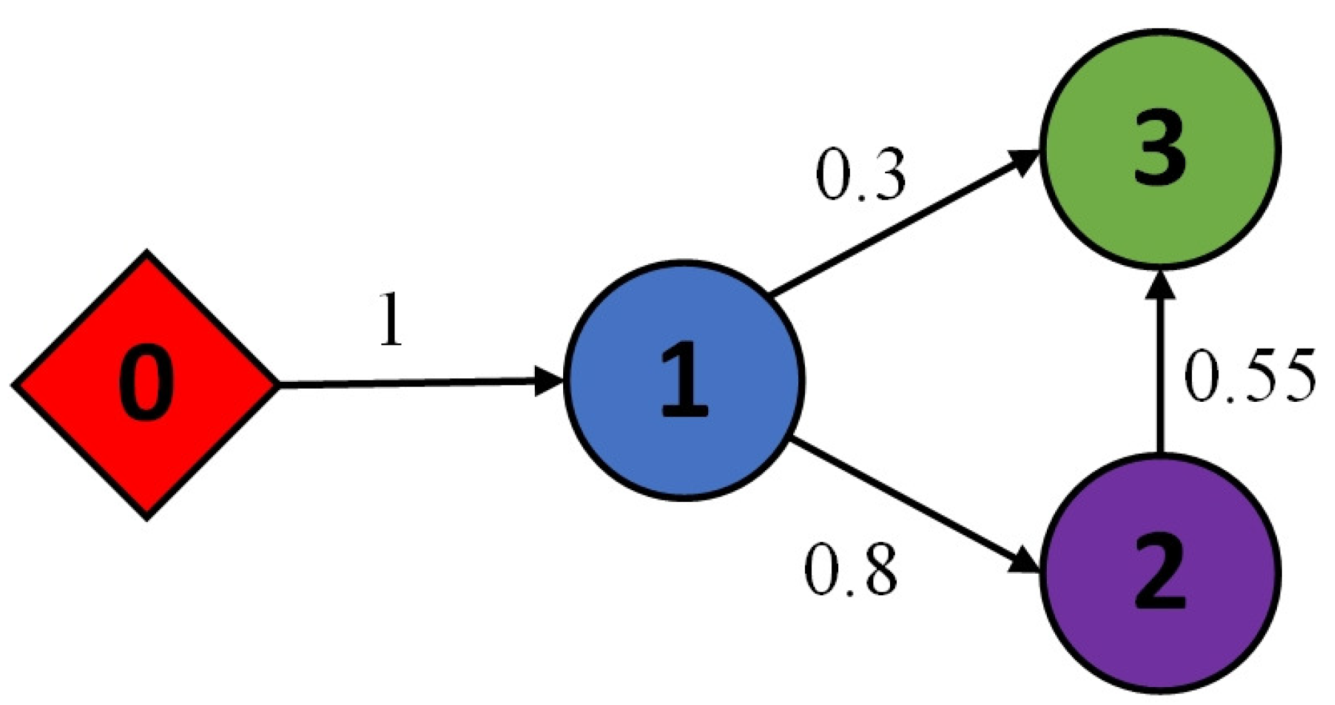
This section explores a formation tracking control study, where three follower UAVs track a virtual leader UAV, aiming to evaluate the effectiveness of the control method proposed in this paper. The communication topology among the UAVs is shown in Figure 2, with the virtual leader UAV labeled as ‘0’ and the follower UAVs labeled ‘1’, ‘2’, and ‘3’.

To comprehensively evaluate the proposed NM-PAETC mechanism, the simulation validation was designed under three distinct operational scenarios: (1) Normal Operation: The multi-UAV system operated under nominal conditions for the first 5 s to establish and maintain the desired formation; (2) Compound Fault and Disturbance Injection: After 5 s, time-varying actuator faults and external unknown disturbances were simultaneously injected to rigorously test the fault-tolerant and disturbance rejection capabilities; (3) Communication-Constrained Validation: Under these faulty conditions, the communication-saving effectiveness of the NM-PAETC mechanism was validated by comparing its trigger events with a traditional continuous-time mechanism.

Remark 2.

In this section, the numerical calculations were performed using ODE45 solver in MATLAB (2022b) with a fixed simulation step size of 0.01 s. Furthermore, the multi-UAV system operated normally for the first 5 s to establish the desired formation, after which time-varying actuator faults and external unknown disturbances were simultaneously injected to rigorously evaluate the fault-tolerant performance and disturbance resilience capabilities of the proposed NM-PAETC mechanism.

The developed adaptive event-triggered control method was as follows:

$$\begin{array}{cccc}& & \hfill \begin{array}{cc}\hfill {\alpha }_{k,\Im ,1}=& {\displaystyle \frac{1}{b_k+D_k}}\left(-r_{k,\Im ,1}{e}_{k,\Im ,1}^{2q-1}-f_{k,\Im ,1}{e}_{k,\Im ,1}^3\right)+{\displaystyle \frac{1}{b_k+D_k}}\left(D_k{\dot{x}}_0+{\displaystyle \sum _{g=1}^N}{a}_{kg}{\dot{x}}_g\right)\hfill \end{array}& \end{array}$$

(84)

$$\begin{array}{cccc}& & \hfill \begin{array}{cc}\hfill {\overline{\alpha }}_{k,\Im ,2}=& r_{k,\Im ,2}{e}_{k,\Im ,2}^{2q-1}+f_{k,\Im ,2}{e}_{k,\Im ,2}^3+{\widehat{d}}_{k,\Im }-{\dot{\alpha }}_{k,\Im ,1}+\left(b_k+D_k\right)e_{k,\Im ,1}\hfill \\ & +{\widehat{\gamma }}_{k,\Im }tanh\left({\displaystyle \frac{e_{k,\Im ,2}}{{\beta }_{k,\Im }}}\right)\hfill \end{array}& \end{array}$$

(85)

$$\begin{array}{cccc}& & \hfill {\dot{\widehat{\varsigma }}}_{k,\Im }={\eta }_{k,\Im }{\overline{\alpha }}_{k,\Im ,2}{e}_{k,\Im ,2}-{\mathcal{l}}_{k,\Im }{\widehat{\varsigma }}_{k,\Im }-{\displaystyle \frac{{\mathcal{l}}_{k,\Im }}{{\eta }_{k,\Im }}}{\widehat{\varsigma }}_{k,\Im }^3& \end{array}$$

(86)

$$\begin{array}{cccc}& & \hfill {\dot{\widehat{\gamma }}}_{k,\Im }={\mu }_{k,\Im }{e}_{k,\Im ,2}tanh\left({\displaystyle \frac{e_{k,\Im ,2}}{{\beta }_{k,\Im }}}\right)-{\iota }_{k,\Im }{\widehat{\gamma }}_{k,\Im }-{\displaystyle \frac{{\iota }_{k,\Im }}{{\mu }_{k,\Im }}}{\widehat{\gamma }}_{k,\Im }^3& \end{array}$$

(87)

$$\begin{array}{cccc}& & \hfill {\alpha }_{k,\Im ,2}=-{\displaystyle \frac{e_{k,\Im ,2}{\widehat{\varsigma }}_{k,\Im }^2{\overline{\alpha }}_{k,\Im ,2}^2}{\sqrt{e_{k,\Im ,2}^2{\widehat{\varsigma }}_{k,\Im }^2{\overline{\alpha }}_{k,\Im ,2}^2+l_{k,\Im }^2}}}(\Im =1,2,3)& \end{array}$$

(88)

$$\begin{array}{cccc}& & \hfill {\overline{u}}_{k,v,1}\left(t\right)={\nu }_{k,v,1}\left(t_s^{k,v}\right),t\in \left[t_s^{k,v},t_{s+1}^{k,v}\right)& \end{array}$$

(89)

$$\begin{array}{cccc}& & \hfill t_{s+1}^{k,v}=\left\{\begin{array}{ccc}& t_s^{k,1}+t_{step},\hfill & \hfill {\dot{\lambda }}_{k,v}\left(t\right)>M_{k,v,3}\\ & & \\ & t_s^{k,v}+{\displaystyle \frac{{\varpi }_{k,v}\left|{\overline{u}}_{k,v,1}\left(t\right)\right|+M_{k,v,1}}{max\left\{M_{k,v,2},{\lambda }_{k,v}\left(t\right)\right\}}},\hfill & \hfill {\dot{\lambda }}_{k,v}\left(t\right)\le M_{k,v,3}\end{array}\right.& \end{array}$$

(90)

$$\begin{array}{cccc}& & \hfill {\nu }_{k,v,1}\left(t\right)={\alpha }_{k,v,2}-{\displaystyle \frac{1}{2}}{e}_{k,v,2}& \end{array}$$

(91)

$$\begin{array}{cccc}& & \hfill {\alpha }_{k,\Re ,1}=-r_{k,\Re }{e}_{k,\Re ,1}-f_{k,\Re }{e}_{k,\Re ,1}+{\dot{\varphi }}_{k,d}\left(\Re =4,5,6\right)& \end{array}$$

(92)

$$\begin{array}{cccc}& & \hfill {\alpha }_{k,\Re ,2}=-{\displaystyle \frac{I_{k,\wp }{e}_{k,\Re ,2}{\widehat{\varsigma }}_{k,\Re }^2{\overline{\alpha }}_{k,\Re ,2}^2}{\sqrt{e_{k,\Re ,2}^2{\widehat{\varsigma }}_{k,\Re }^2{\overline{\alpha }}_{k,\Re ,2}^2+l_{k,\Re }^2}}}\left(\wp =1,2,3\right)& \end{array}$$

(93)

$$\begin{array}{cccc}& & \hfill \begin{array}{cc}\hfill {\overline{\alpha }}_{k,\Re ,2}=& r_{k,\Re ,2}{e}_{k,\Re ,2}^{2q-1}+f_{k,\Re ,2}{e}_{k,\Re ,2}^3+e_{k,\Re ,1}+{\widehat{d}}_{k,\Re }-{\dot{\alpha }}_{k,\Re ,1}+{I^{-1}}_{k,\wp }{\widehat{\gamma }}_{k,\Re }tanh\left({\displaystyle \frac{e_{k,\Re ,2}}{{\beta }_{k,\Re }}}\right)\hfill \end{array}& \end{array}$$

(94)

$$\begin{array}{cccc}& & \hfill {\dot{\widehat{\varsigma }}}_{k,\Re }={\eta }_{k,\Re }{\overline{\alpha }}_{k,\Re ,2}{e}_{k,\Re ,2}-{\mathcal{l}}_{k,\Re }{\widehat{\varsigma }}_{k,\Re }-{\displaystyle \frac{{\mathcal{l}}_{k,\Re }}{{\eta }_{k,\Re }}}{\widehat{\varsigma }}_{k,\Re }^3& \end{array}$$

(95)

$$\begin{array}{cccc}& & \hfill \begin{array}{cc}\hfill {\dot{\widehat{\gamma }}}_{k,\Re }=& {I^{-1}}_{k,\wp }{\mu }_{k,\Re }{e}_{k,\Re ,2}tanh\left({\displaystyle \frac{e_{k,\Re ,2}}{{\beta }_{k,\Re }}}\right)-{\iota }_{k,\Re }{\widehat{\gamma }}_{k,\Re }-{\displaystyle \frac{{\iota }_{k,\Re }}{{\mu }_{k,\Re }}}{\widehat{\gamma }}_{k,\Re }^3\hfill \end{array}& \end{array}$$

(96)

The actuator operates normally for 5 s, and the failure model after 5 s was given by:

$$\begin{array}{cccc}& & \hfill h_{k,1}\left(t\right)=\left\{\begin{array}{cc}1,\hfill & t<5s\hfill \\ 0.5+0.5e^{-0.5\left(t-5\right)},\hfill & t\ge 5s\hfill \end{array}\right.& \end{array}$$

(97)

$$\begin{array}{cccc}& & \hfill {ħ}_{k,1}\left(t\right)=\left\{\begin{array}{cc}0,\hfill & t<5s\hfill \\ -0.4+0.4e^{-0.5\left(t-5\right)},\hfill & t\ge 5s\hfill \end{array}\right.& \end{array}$$

(98)

Assuming the required attitude angles to satisfy Equation (1) are ${\varphi }_{k,d}$,${\theta }_{k,d}$, and ${\psi }_{k,d}$, it is necessary to solve for ${\theta }_k$ and ${\psi }_k$ to achieve tracking of ${\theta }_{k,d}$ and ${\psi }_{k,d}$. Based on the state equations of the position subsystem, the auxiliary position controller can be derived as $u_{k,x}={\widehat{\varsigma }}_{k,1}{\overline{u}}_{k,x,1}+{\widehat{\gamma }}_{k,1}$, $u_{k,y}={\widehat{\varsigma }}_{k,2}{\overline{u}}_{k,y,1}+{\widehat{\gamma }}_{k,2}$ and $u_{k,z}={\widehat{\varsigma }}_{k,3}{\overline{u}}_{k,z,1}+{\widehat{\gamma }}_{k,3}$.

$$\begin{array}{cccc}& & \hfill \left\{\begin{array}{c}{u}_{k,x}={\displaystyle \frac{h_{k,1}\left(t\right){\overline{u}}_{k,1}+{ħ}_{k,1}\left(t\right)}{m_k}}\left(cos{\varphi }_{k}sin{\theta }_{k}cos{\psi }_k+sin{\varphi }_{k}sin{\psi }_k\right)\hfill \\ u_{k,y}={\displaystyle \frac{h_{k,2}\left(t\right){\overline{u}}_{k,1}+{ħ}_{k,2}\left(t\right)}{m_k}}\left(sin{\varphi }_{k}sin{\theta }_{k}cos{\psi }_k-cos{\varphi }_{k}sin{\psi }_k\right)\hfill \\ u_{k,z}={\displaystyle \frac{h_{k,3}\left(t\right){\overline{u}}_{k,1}+{ħ}_{k,3}\left(t\right)}{m_k}}cos{\varphi }_{k}cos{\theta }_k-g\hfill \end{array}\right.& \end{array}$$

(99)

Using ${sin}^2\left(·\right)+{cos}^2(·)=1$ and (99), $u_{k,1}$ and the desired target states ${\varphi }_{k,d}$ and ${\theta }_{k,d}$ can be expressed as follows:

$$\begin{array}{cccc}& & \hfill \left\{\begin{array}{c}{u}_{k,1}=m_k\sqrt{u_{k,x}^2+u_{k,y}^2+{(u_{k,z}+g)}^2}\hfill \\ {\varphi }_{k,d}=arcsin\left({\displaystyle \frac{m_k}{u_{k,x}}}\left(u_{k,x}sin\left({\psi }_{k,d}\right)-u_{k,y}cos\left({\psi }_{k,d}\right)\right)\right)\hfill \\ {\theta }_{k,d}=arctan\left({\displaystyle \frac{m_k}{u_{k,z}+g}}\left(u_{k,x}cos\left({\psi }_{k,d}\right)+u_{k,y}sin\left({\psi }_{k,d}\right)\right)\right)\hfill \end{array}\right.& \end{array}$$

(100)

In the example validation, the parameter design for QUAVs was as follows (similar to [14]): $m_k=2\mathrm{kg}$, $K_{k,1}=K_{k,2}=K_{k,3}=0.01\mathrm{N}·\mathrm{s}/\mathrm{m}$, $K_{k,4}=K_{k,5}=K_{k,6}=0.001\mathrm{N}·\mathrm{s}/(\mathrm{rad}·\mathrm{m})$, ${\aleph }_{k,1}=0.5sin\left(t\right)+0.5sin\left(x_k\right)\mathrm{N}$, ${\aleph }_{k,2}=0.5sin\left(t\right)+0.5sin\left(y_k\right)\mathrm{N}$, ${\aleph }_{k,3}=0.5sin\left(t\right)+0.5sin\left(z_k\right)\mathrm{N}$, $I_{k,x}=1.5\mathrm{N}·{\mathrm{s}}^2/\mathrm{rad}$, ${\aleph }_{k,4}=0.5sin\left(t\right)+0.5sin\left({\theta }_k\right)\mathrm{N}$, $I_{k,y}=1.5\mathrm{N}·{\mathrm{s}}^2/\mathrm{rad}$, ${\aleph }_{k,5}=0.5sin\left(t\right)+0.5sin\left({\psi }_k\right)\mathrm{N}$, $I_{k,z}=1.5\mathrm{N}·{\mathrm{s}}^2/\mathrm{rad}$, ${\aleph }_{k,6}=0.5sin\left(t\right)+0.5sin\left({\varphi }_k\right)\mathrm{N}$, $q=\raisebox{1ex}{$4$}\!\left/ \!\raisebox{-1ex}{$5$}\right.$

The composite disturbances were denoted as $d_{k,1}=-{\displaystyle \frac{K_{k,1}}{m_k}}{\dot{x}}_k+{\displaystyle \frac{{\aleph }_{k,1}}{m_k}}$, $d_{k,2}=-{\displaystyle \frac{K_{k,2}}{m_k}}{\dot{y}}_k+{\displaystyle \frac{{\aleph }_{k,2}}{m_k}}$, $d_{k,3}=-{\displaystyle \frac{K_{k,3}}{m_k}}{\dot{z}}_k+{\displaystyle \frac{{\aleph }_{k,3}}{m_k}}$, $d_{k,4}={\dot{\theta }}_k{\dot{\psi }}_k{\displaystyle \frac{I_{k,y}-I_{k,z}}{I_{k,x}}}-{\displaystyle \frac{K_{k,4}}{I_{k,x}}}{\dot{\varphi }}_k+{\displaystyle \frac{{\aleph }_{k,4}}{I_{k,x}}}$, $d_{k,5}={\dot{\varphi }}_k{\dot{\psi }}_k{\displaystyle \frac{I_{k,z}-I_{k,x}}{I_{k,y}}}-{\displaystyle \frac{K_{k,5}}{I_{k,y}}}{\dot{\varphi }}_k+{\displaystyle \frac{{\aleph }_{k,5}}{I_{k,y}}}$, $d_{k,6}={\dot{\varphi }}_k{\dot{\theta }}_k{\displaystyle \frac{I_{k,x}-I_{k,z}}{I_{k,z}}}-{\displaystyle \frac{K_{k,6}}{I_{k,z}}}{\dot{\varphi }}_k+{\displaystyle \frac{{\aleph }_{k,6}}{I_{k,z}}}$. The controller parameters were $r_{1,1,1}=r_{1,2,1}=0.1$, $f_{k,v,1}=f_{k,v,1}=5$, $r_{1,3,1}=4$, $f_{1,3,1}=2$, $r_{k,v,2}=15$, $f_{1,1,2}=f_{1,2,2}=220$, $f_{1,3,3}=65$, $r_{1,4,1}=r_{1,5,1}=r_{1,6,1}=2$, $f_{1,4,1}=f_{1,5,1}=f_{1,6,1}=15$, $r_{1,4,2}=r_{1,5,2}=r_{1,6,2}=1$, $f_{1,4,2}=f_{1,5,2}=f_{1,6,2}=40$, $r_{k,J,1}=1(k=2,3;J=1,2)$, $r_{k,3,1}=f_{k,3,1}=2$, $r_{k,J,2}=2$, $f_{k,1,2}=225$, $f_{k,2,2}=210$, $f_{k,3,2}=60$, $r_{k,E,J}=0.1(k=2,3;E=4,5)$, $f_{k,E,1}=30$, $r_{k,6,J}=2$$(k=2,3;J=4,5)$, $f_{k,6,1}=20$, $r_{k,6,2}=20$, $f_{k,6,2}=35$, ${\eta }_{k,1,1}=0.001$, ${\mathcal{l}}_{k,1}=0.001$, ${\mu }_{k,1}=0.01$, ${\beta }_{k,1}=0.01$, ${\iota }_{k,1,1}=1$, $l_{k,1,1}=0.01$, ${\kappa }_{k,v,1}=13$, ${\kappa }_{k,v,2}=0.01$, ${\kappa }_{k,v,3}=11$, ${\kappa }_{k,v,4}=10$. The system’s initial states and attitude are shown in

Table 2. Initial states of UAVs.

Translational Initial States
Case	${\mathit{x}}_{\mathit{k},\mathit{1}}\left(\mathit{0}\right)$	${\mathit{x}}_{\mathit{k},\mathit{2}}\left(\mathit{0}\right)$	${\mathit{y}}_{\mathit{k},\mathit{1}}\left(\mathit{0}\right)$	${\mathit{y}}_{\mathit{k},\mathit{2}}\left(\mathit{0}\right)$	${\mathit{z}}_{\mathit{k},\mathit{1}}\left(\mathit{0}\right)$	${\mathit{z}}_{\mathit{k},\mathit{2}}\left(\mathit{0}\right)$
UAV 1	$2.5\mathrm{m}$	$0\mathrm{m}/\mathrm{s}$	$8.9\mathrm{m}$	$0\mathrm{m}/\mathrm{s}$	$0\mathrm{m}$	$0\mathrm{m}/\mathrm{s}$
UAV 2	$3.6\mathrm{m}$	$0\mathrm{m}/\mathrm{s}$	$9.8\mathrm{m}$	$0\mathrm{m}/\mathrm{s}$	$0\mathrm{m}$	$0\mathrm{m}/\mathrm{s}$
UAV 3	$4.7\mathrm{m}$	$0\mathrm{m}/\mathrm{s}$	$10.9\mathrm{m}$	$0\mathrm{m}/\mathrm{s}$	$0\mathrm{m}$	$0\mathrm{m}/\mathrm{s}$
Rotational Initial States
Case	${\mathit{\varphi }}_{\mathit{k}}\left(\mathit{0}\right)$	${\mathit{\omega }}_{\mathit{k},\mathit{\varphi }}\left(\mathit{0}\right)$	${\mathit{\theta }}_{\mathit{k}}\left(\mathit{0}\right)$	${\mathit{\omega }}_{\mathit{k},\mathit{\theta }}\left(\mathit{0}\right)$	${\mathit{\psi }}_{\mathit{k}}\left(\mathit{0}\right)$	${\mathit{\omega }}_{\mathit{k},\mathit{\psi }}\left(\mathit{0}\right)$
UAV 1	$0.1\mathrm{rad}$	$0\mathrm{rad}/\mathrm{s}$	$0.1\mathrm{rad}$	$0\mathrm{rad}/\mathrm{s}$	$0.4\mathrm{rad}$	$0\mathrm{rad}/\mathrm{s}$
UAV 2	$0.1\mathrm{rad}$	$0\mathrm{rad}/\mathrm{s}$	$0.1\mathrm{rad}$	$0\mathrm{rad}/\mathrm{s}$	$0.4\mathrm{rad}$	$0\mathrm{rad}/\mathrm{s}$
UAV 3	$0.1\mathrm{rad}$	$0\mathrm{rad}/\mathrm{s}$	$0.1\mathrm{rad}$	$0\mathrm{rad}/\mathrm{s}$	$0.4\mathrm{rad}$	$0\mathrm{rad}/\mathrm{s}$

.

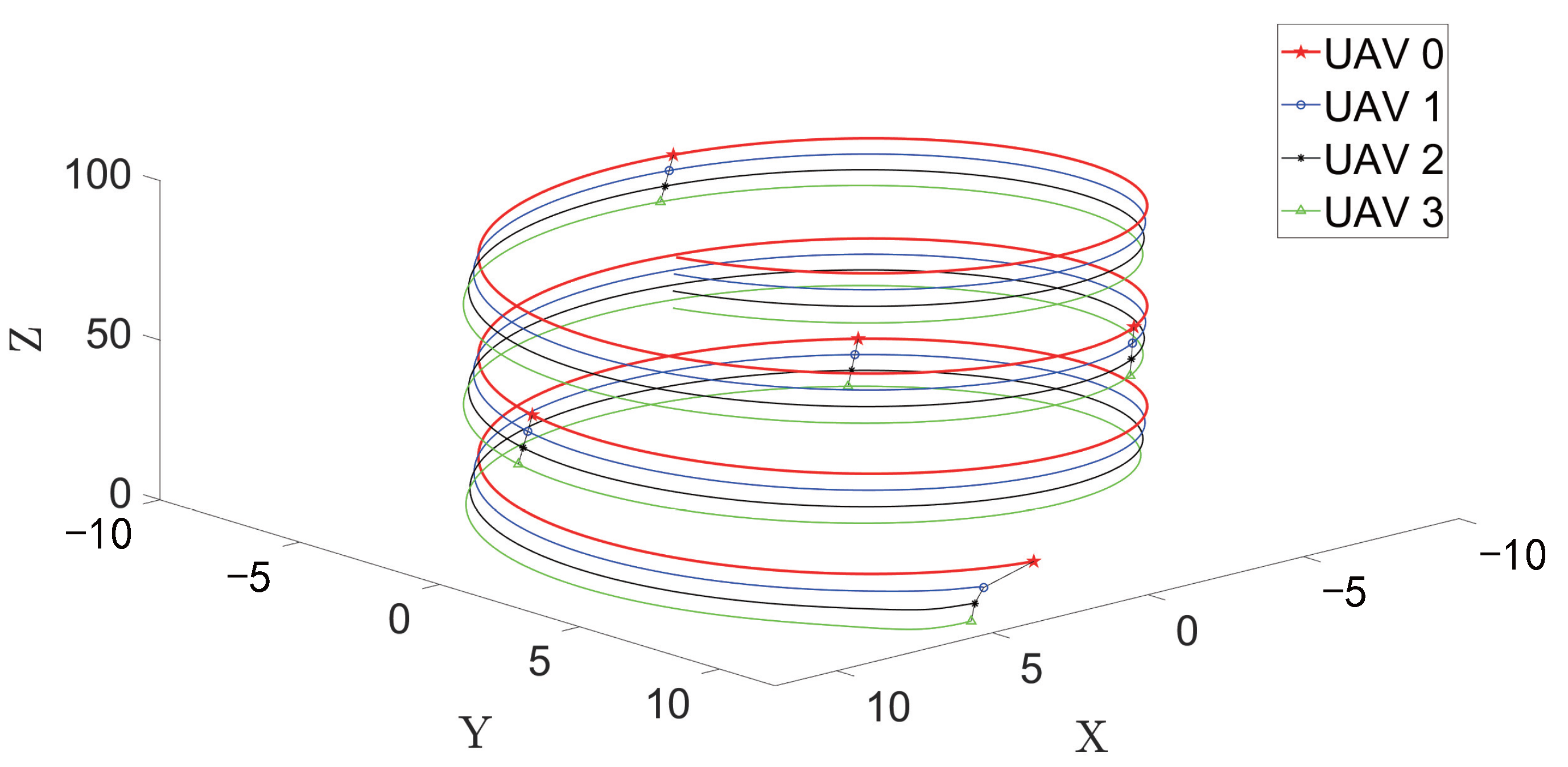
The simulation results are shown in Figure 3, Figure 4, Figure 5, Figure 6, Figure 7 and Figure 8; Figure 3 illustrates the trajectory of three QUAVs following the virtual leader. The multi-UAV system operated normally during the first 0.5 s, achieving a linear formation and following the predetermined trajectory. After 5 s, even with time-varying failures occurring in each UAV, the system maintained the linear formation and continued to follow the designated path. Figure 4 illustrate the system outputs, where the positions of each UAV in the different directions successfully formed the required formation.

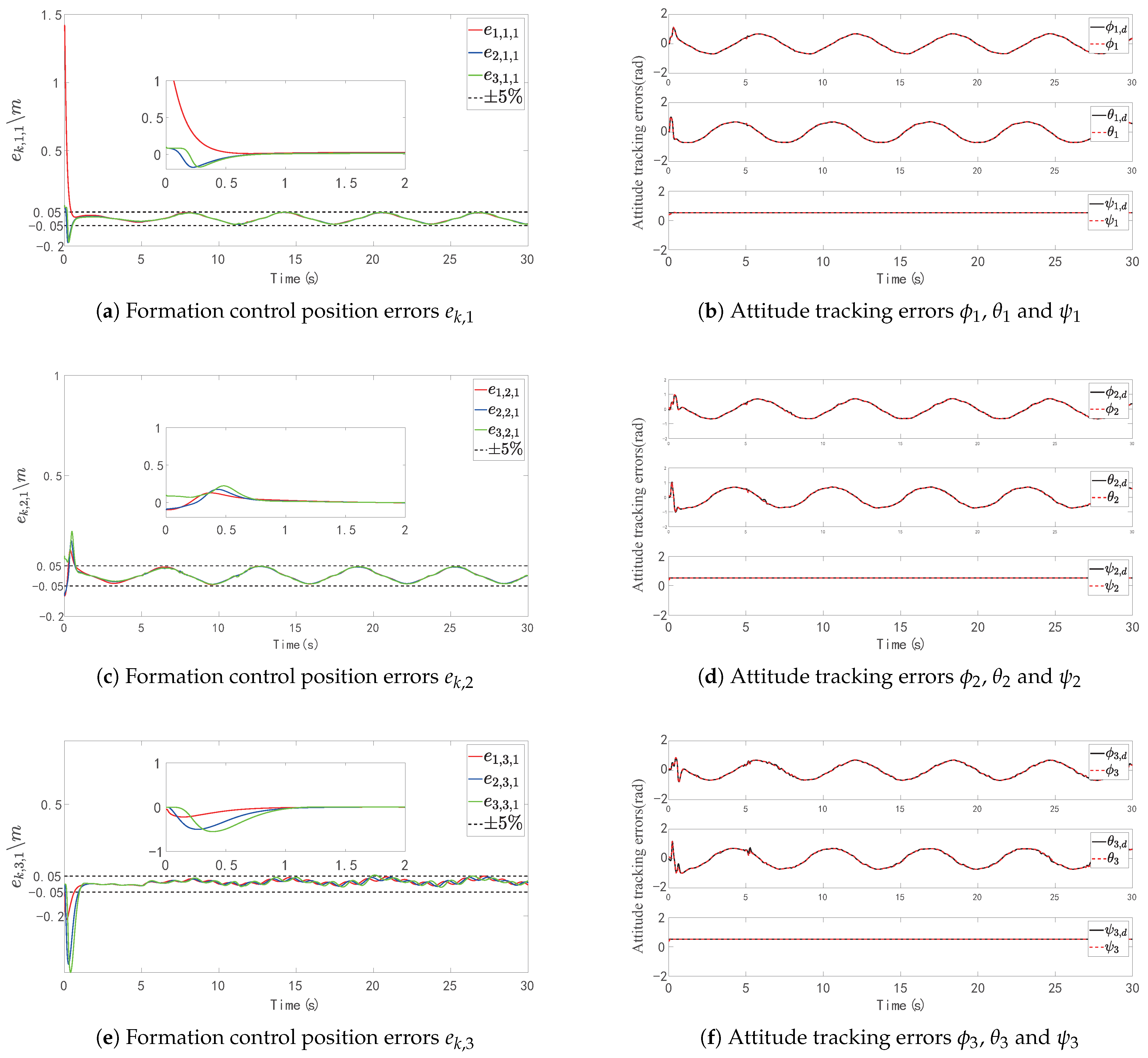
Additionally, the angles necessary to ensure system formation and stability were derived from Equation (100) and tracked accordingly. Figure 5a,c,e represent formation errors. Figure 5b,d,f show that the derived angles closely align with the ideal angles, thus confirming the feasibility of the proposed derivation method. The system’s formation error can be maintained within a range of $\pm 5\%$ within 1 s, while the angle tracking error can similarly be kept within a range of $\pm 0.05$ rad∖s within 0.5 s. The system’s position and attitude are precisely controlled, which also highlights the advantages of using fixed-time control methods.

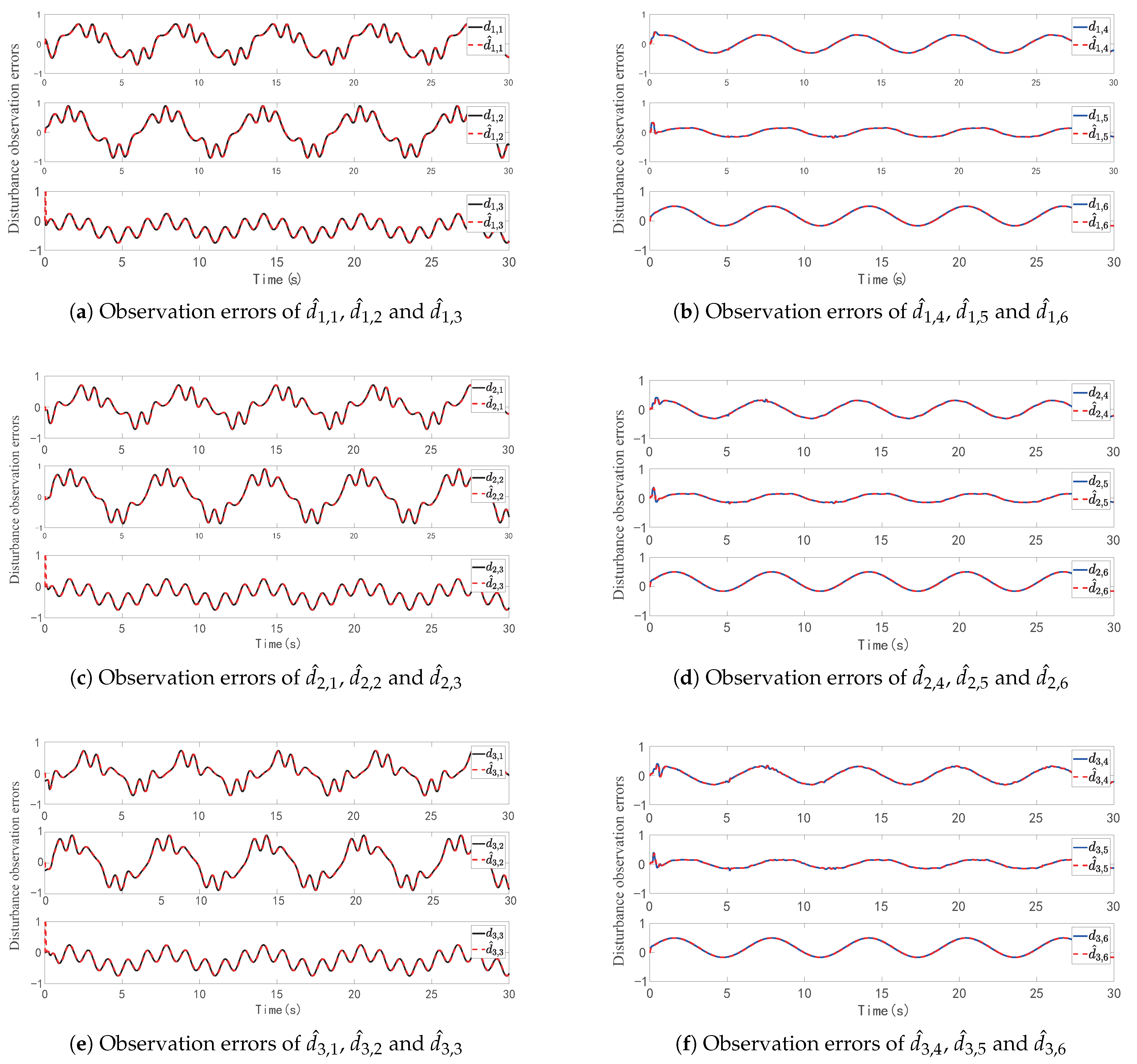
The external disturbances and the observer’s measurements of the system are shown in Figure 6. The observer effectively estimates external disturbances within approximately 0.5 s, with the resulting estimation errors remaining within acceptable limits. It is capable of estimating and compensating for external disturbances effectively, thereby eliminating their impact on the system and significantly enhancing its disturbance resistance. The application of the observer leads to a reduction in the system’s position formation error and reference angle tracking error. Unlike relying solely on the robustness of the controller to address external disturbances, the system with the fixed-time disturbance observer can effectively counteract external disturbances, enabling the proposed control method to better handle variations in disturbances and maintain the stability and precision of formation flight.

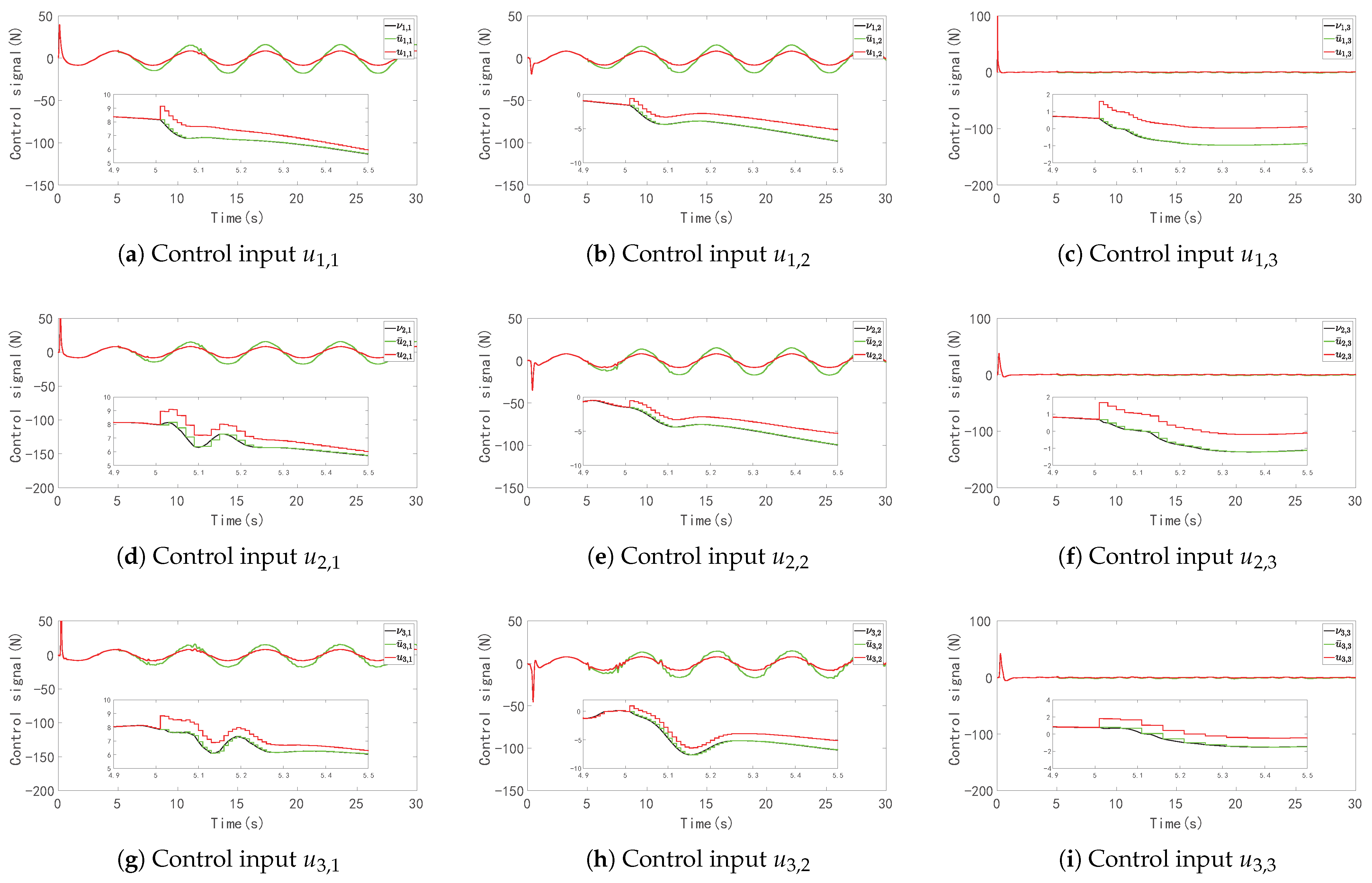
Figure 7 illustrates the control signals of each actuator. It can be observed that the fault occurs after 5 s, with a significant discrepancy between the actuator’s input and output. The red line represents the output control signal of the faulty actuator, highlighting the impact of the fault on system performance. However, the designed controller quickly mitigates these effects, ensuring rapid recovery of formation control while keeping the formation error within the allowable range.

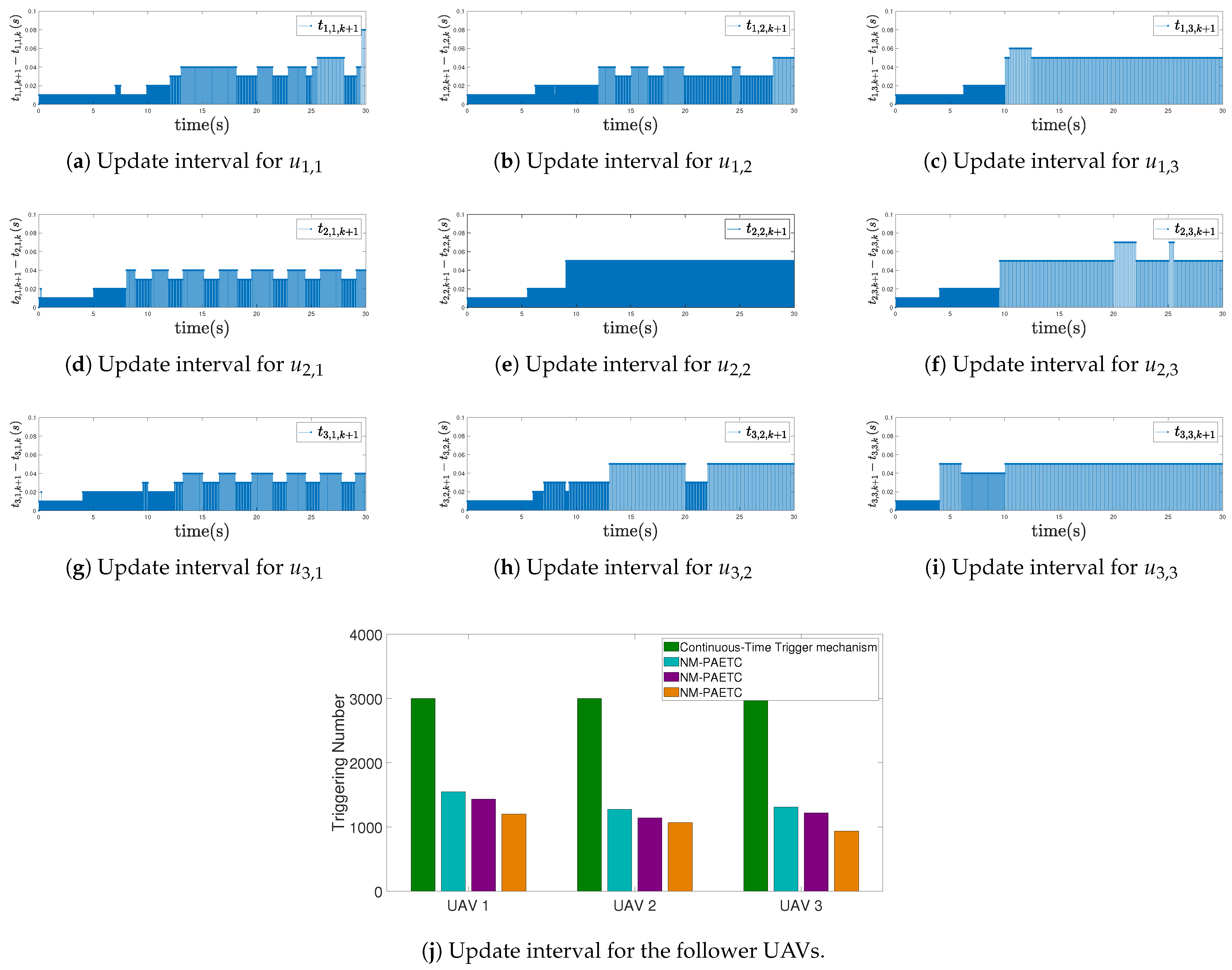
Figure 8 shows the trigger interval times under the NM-PAETC mechanism, with the fixed step size of 0.01 s chosen in the experiment. The bandwidth resource saving rate was calculated by the ratio of the reduced number of trigger events to the number of triggers required by the continuous-time control method. While achieving bandwidth savings, the system maintains stable formation control, with the desired attitude angles closely matching the actual attitude angles. Clearly, the proposed NM-PAETC method not only effectively reduces communication resource consumption but also ensures formation control of the quadrotor UAVs under ideal attitude angles. Additionally, the detailed triggering data and the percentage of bandwidth savings are shown in

Table 3. Table of event triggers for each UAV.

Item	Actuator 1	Actuator 2	Actuator 3
CTTM	3000	3000	3000
Percentage	/	/	/
UAV 1	1549	1438	1200
Percentage	48%	52%	60%
UAV 2	1276	1145	1071
Percentage	58%	62%	64%
UAV 3	1314	1222	940
Percentage	56%	59%	69%

.

To further clarify the novelty and practical advantages of the proposed method,

Table 4. Comparison with representative existing studies.

Ref.	Actuator Fault	Disturbance Observer	Fixed- Time	Event- Triggered	Zeno- Free	Online Requirement
[5]	✓	×	✓	×	×	×
[13]	✓	✓	×	✓	×	×
[14]	✓	✓	✓	×	×	×
[16]	×	✓	✓	×	×	×
[18]	×	✓	×	✓	×	×
[29]	✓	×	✓	×	×	×
Proposed	✓	✓	✓	✓	✓	×

presents comparisons with representative studies cited in this manuscript. Existing studies mainly focus on specific aspects, such as actuator fault compensation [5], disturbance observation [14,16], or event-triggered communication strategies [13,18]. However, only limited attention has been given to simultaneously integrating actuator fault accommodation, fixed-time disturbance estimation, adaptive event-triggered communication, and Zeno-free guarantees into a unified framework. Compared with existing methods, the proposed approach combines a fixed-time disturbance observer with the NM-PAETC mechanism, while accounting for time-varying actuator failures and communication constraints. Furthermore, the proposed control scheme does not require online optimization or iterative numerical procedures, which reduces computational burden and enhances practical real-time applicability.

Remark 3.

To further clarify the methodological advantages of the proposed control scheme, a comparison with representative finite/fixed-time observer-based and adaptive/NN-based FTC methods is provided. Existing finite-time observer-based methods can estimate unknown disturbances within a finite time, but their convergence time is generally related to the initial estimation error. Fixed-time observer-based methods improve this issue, although they are often not simultaneously combined with adaptive event-triggered communication and actuator fault compensation. In addition, adaptive or NN-based FTC methods can compensate for unknown nonlinearities and actuator faults, but they usually introduce additional adaptive parameters or neural network weights, which may increase the online computational burden. In contrast, the proposed method integrates fixed-time disturbance observation, adaptive compensation for time-varying actuator faults, and the NM-PAETC mechanism into a unified framework. Therefore, the proposed control scheme can ensure fixed-time convergence, reduce communication resource consumption, and avoid Zeno behavior without relying on online optimization or complex NN approximation structures.

From the simulation results presented above, the theoretical analysis is validated, demonstrating that stable formation control in quadrotor UAVs can be achieved within a fixed time, even under time-varying actuator failures.

6. Conclusions

This work presented a periodic adaptive event-triggered fixed-time fault-tolerant control method for QUAV systems, effectively addressing the challenges of actuator faults, unknown external disturbances, and limited communication resources. Theoretical analysis confirmed that: (1) time-varying actuator faults were accurately estimated and compensated; (2) both system and observer errors converged within a fixed time; (3) the communication burden was notably reduced, enabling the QUAV to maintain formation control at the desired attitude angles while avoiding Zeno behavior. The effectiveness of the proposed method was further validated through simulation results. Furthermore, extending the proposed control framework and the NM-PAETC mechanism to other multi-rotor UAV configurations with redundant actuators would be a highly interesting direction for our future research.

References

1. Ullah, S.; Khan, Q.; Mehmood, A.; Kirmani, S.A.M.; Mechali, O. Neuro-adaptive fast integral terminal sliding mode control design with variable gain robust exact differentiator for under-actuated quadcopter UAV. ISA Trans. 2022, 120, 293–304. [Google Scholar] [PubMed]
2. Song, X.; Shen, L.; Chen, F. Adaptive position control using backstepping technique for the leader-follower multiple quadrotor unmanned aerial vehicle formation. Int. J. Adapt. Control Signal Process. 2024, 38, 3121–3133. [Google Scholar]
3. Yan, Y.; Zhang, H.; Sun, J.; Ming, Z. Optimal fuzzy event-triggered fault-tolerant control of fractional-order nonlinear stochastic systems. Inf. Sci. 2024, 678, 120877. [Google Scholar]
4. Ma, Z.; Gong, H.; Wang, X. Fault-Tolerant Event-Triggrred Control for Multiple UAVs with Predefined Tracking Performance. Drones 2024, 8, 25. [Google Scholar]
5. Miao, Q.; Zhang, K.; Jiang, B. Fixed-Time Collision-Free Fault-Tolerant Formation Control of Multi-UAVs Under Actuator Faults. IEEE Trans. Cybern. 2024, 54, 3679–3691. [Google Scholar] [PubMed]
6. Jiang, D.; Wen, G.; Peng, Z.; Huang, T.; Rahmani, A. Fully Distributed Dual-Terminal Event-Triggered Bipartite Output Containment Control of Heterogeneous Systems Under Actuator Faults. IEEE Trans. Syst. Man. Cybern. Syst. 2022, 52, 5518–5531. [Google Scholar]
7. Zhao, W.; Liu, H.; Lewis, F.L. Data-Driven Fault-Tolerant Control for Attitude Synchronization of Nonlinear Quadrotors. IEEE Trans. Autom. Control 2021, 66, 5584–5591. [Google Scholar]
8. Hua, Y.; Dong, X.; Li, Q.; Ren, Z. Distributed Fault-Tolerant Time-Varying Formation Control for Second-Order Multi-Agent Systems with Actuator Failures and Directed Topologies. IEEE Trans. Circuits Syst. II Express Briefs 2018, 65, 774–778. [Google Scholar]
9. Chang, S.; Wang, Y.; Zuo, Z. Fixed-time formation-containment control for uncertain multi- agent systems with varying gain extended state observer. Inf. Sci. 2022, 612, 759–779. [Google Scholar]
10. Liu, K.; Wang, R.; Wang, X.; Wang, X. Anti-saturation adaptive finite-time neural network based fault-tolerant tracking control for a quadrotor UAV with external disturbances. Aerosp. Sci. Technol. 2021, 115, 106790. [Google Scholar]
11. Sanwale, J.; Dahiya, S.; Trivedi, P.; Kothari, M. Robust fault-tolerant adaptive integral dynamic sliding mode control using finite-time disturbance observer for coaxial octorotor UAVs. Control Eng. Pract. 2023, 135, 105495. [Google Scholar] [CrossRef]
12. Altan, A.; Hacıoğlu, R. Model predictive control of three-axis gimbal system mounted on UAV for real-time target tracking under external disturbances. Mech. Syst. Signal Process. 2020, 138, 106548. [Google Scholar]
13. Wang, L.; Li, A.; Xiao, C.; Wang, C.; Zabolotnov, Y. Distributed adaptive disturbance observer-based multi-channel event-triggered finite-time coordinated control for multi-UAVs with actuator failures. Aerosp. Sci. Technol. 2024, 151, 109319. [Google Scholar]
14. Liu, K.; Wang, R.; Zheng, S.; Dong, S.; Sun, G. Fixed-time disturbance observer-based robust fault-tolerant tracking control for uncertain quadrotor UAV subject to input delay. Nonlinear Dyn. 2022, 107, 2363–2390. [Google Scholar]
15. Zhang, N.; Xia, J.; Park, J.H.; Zhang, J.; Shen, H. Improved disturbance observer-based fixed-time adaptive neural network consensus tracking for nonlinear multi-agent systems. Neural Netw. 2023, 162, 490–501. [Google Scholar] [PubMed]
16. Zhang, B.; Sun, X.; Lv, M.; Liu, S. Distributed Coordinated Control for Fixed-Wing UAVs with Dynamic Event-Triggered Communication. IEEE Trans. Veh. Technol. 2022, 71, 4665–4676. [Google Scholar]
17. Wang, J.; Bi, C.; Wang, D.; Kuang, Q.; Wang, C. Finite-time distributed event-triggered formation control for quadrotor UAVs with experimentation. ISA Trans. 2022, 126, 585–596. [Google Scholar] [PubMed]
18. Wang, C.; Yang, N.; Li, W.; Liang, M. Event-triggered finite-time fuzzy tracking control for a time-varying state constrained quadrotor system based on disturbance observer. Aerosp. Sci. Technol. 2024, 151, 109329. [Google Scholar]
19. Hu, C.; Zhao, L.; Qu, G. Event-Triggered Model Predictive Adaptive Dynamic Programming for Road Intersection Path Planning of Unmanned Ground Vehicle. IEEE Trans. Veh. Technol. 2021, 70, 11228–11243. [Google Scholar] [CrossRef]
20. Babazadeh, H.; Baradarannia, M.; Hashemzadeh, F. Event-triggered surrounding adaptive control of nonlinear multi-agent systems. ISA Trans. 2022, 128, 44–57. [Google Scholar] [PubMed]
21. Liu, Z.; Zhang, A.; Qiu, J.; Li, Z. Event-triggered control of second-order nonlinear multi-agent systems with directed topology. Neurocomputing 2021, 452, 820–826. [Google Scholar]
22. Yao, D.; Dou, C.; Yue, D.; Zhao, N.; Zhang, T. Event-triggered adaptive consensus tracking control for nonlinear switching multi-agent systems. Neurocomputing 2020, 415, 157–164. [Google Scholar]
23. Wang, L.; Dong, J. Adaptive Fuzzy Consensus Tracking Control for Uncertain Fractional-Order Multiagent Systems with Event-Triggered Input. IEEE Trans. Fuzzy Syst. 2022, 30, 310–320. [Google Scholar]
24. He, J.; Liao, J. Formation tracking control with disturbance rejection in leader-follower multi-agent systems under dynamic event-triggered mechanism. Eng. Appl. Artif. Intell. 2024, 133, 108441. [Google Scholar]
25. Jia, J.; Chen, X.; Wang, W.; Liao, H.; Xie, M. Collision avoidance in target encirclement and tracking of unmanned aerial vehicles under a dynamic event-triggered formation control. Control Eng. Pract. 2024, 142, 105781. [Google Scholar]
26. Yu, Z.; Li, Y.; Lv, M.; Pei, B.; Fu, A. Event-Triggered Adaptive Fuzzy Fault-Tolerant Attitude Control for Tailless Flying-Wing UAV with Fixed-Time Convergence. IEEE Trans. Veh. Technol. 2024, 73, 4858–4869. [Google Scholar]
27. Zhan, X.; Lu, R.; Wu, J.; Yan, H. Practical fixed-time multi-group time-varying formation for second-order multi-agent systems with actuator attacks and collision avoidance. Inf. Sci. 2024, 678, 120821. [Google Scholar]
28. Li, B.; Gong, W.; Yang, Y.; Xiao, B.; Ran, D. Appointed Fixed Time Observer-Based Sliding Mode Control for a Quadrotor UAV Under External Disturbances. IEEE Trans. Aerosp. Electron. Syst. 2022, 58, 290–303. [Google Scholar] [CrossRef]
29. Gong, W.; Li, B.; Yang, Y.; Ban, H.; Xiao, B. Fixed-time integral-type sliding mode control for the quadrotor UAV attitude stabilization under actuator failures. Aerosp. Sci. Technol. 2019, 95, 105444. [Google Scholar]
30. Li, S.; Shao, X.; Zhang, W.; Zhang, Q. Distributed Multicircular Circumnavigation Control for UAVs with Desired Angular Spacing. Def. Technol. 2024, 31, 429–446. [Google Scholar] [CrossRef]
31. Blas, L.A.; Davila, J.; Salazar, S.; Bonilla, M. Robust Trajectory Tracking for an Uncertain UAV Based on Active Disturbance Rejection. IEEE Control Syst. Lett. 2022, 6, 1466–1471. [Google Scholar]
32. Zhao, Z.; Wang, X.; Yao, P.; Xu, J.; Yu, J. Fuzzy health degree-based dynamic performance evaluation of quadrotors in the presence of actuator and sensor faults. Nonlinear Dyn. 2019, 95, 2477–2490. [Google Scholar] [CrossRef]
33. Ke, J.; Huang, W.; Wang, J.; Zeng, J. Fixed-time consensus control for multi-agent systems with prescribed performance under matched and mismatched disturbances. ISA Trans. 2022, 119, 135–151. [Google Scholar] [PubMed]
34. Zuo, Z.; Ke, R.; Han, Q.L. Fully distributed adaptive practical fixed-time consensus protocols for multi-agent systems. Automatica 2023, 157, 111248. [Google Scholar]
35. Wang, C.; Lin, Y. Decentralized adaptive tracking control for a class of interconnected nonlinear time-varying systems. Automatica 2015, 54, 16–24. [Google Scholar] [CrossRef]
36. Zhang, H.; Lewis, F.L. Adaptive cooperative tracking control of higher-order nonlinear systems with unknown dynamics. Automatica 2012, 48, 1432–1439. [Google Scholar] [CrossRef]
37. Yang, T.; Kang, H.; Ma, H. Adaptive Fuzzy Fixed-Time Tracking Control for Switched High-Order Multi-Agent Systems with Input Delay. IEEE Trans. Netw. Sci. Eng. 2022, 9, 3492–3503. [Google Scholar]
38. Yang, H.; Ye, D. Observer-Based Fixed-Time Secure Tracking Consensus for Networked High-Order Multiagent Systems Against DoS Attacks. IEEE Trans. Cybern. 2022, 52, 2018–2031. [Google Scholar] [PubMed]
39. Xin, W.; Hong, Y.G. Fault-Tolerant Consensus Tracking Control for Linear Multiagent Systems Under Switching Directed Network. IEEE Trans. Cybern. 2019, 50, 1921–1930. [Google Scholar] [CrossRef]
40. Ren, H.; Ma, H.; Li, H.; Wang, Z. Adaptive Fixed-Time Control of Nonlinear MASs with Actuator Faults. IEEE/CAA J. Autom. Sin. 2023, 10, 1252–1262. [Google Scholar] [CrossRef]
Figure 1. Ground and body coordinate systems.
Actuators 15 00366 g001
Figure 2. System communication topology structure diagram.
Actuators 15 00366 g002
Figure 3. Actual trajectory tracking curves for the UAVs.
Actuators 15 00366 g003
Figure 4. Position control of follower UAVs in the presence of actuator faults. (a) Formation tracking trajectory in the x direction. (b) Formation tracking trajectory in the y direction. (c) Formation tracking trajectory in the z direction.
Actuators 15 00366 g004
Figure 5. Position and attitude tracking errors of the follower UAVs.
Actuators 15 00366 g005
Figure 6. Disturbance observation errors of the follower UAVs.
Actuators 15 00366 g006
Figure 7. Control signals following actuator failures for follower UAVs.
Actuators 15 00366 g007
Figure 8. Update interval of control signals for the follower UAVs.
Actuators 15 00366 g008