Article

Weak Disturbance Decoupling for Strict Feedback-like Systems with Unknown Nonlinearities and Its Application in Manipulators

1
School of Rail Transportation, Shandong Jiaotong University, Jinan 250357, China
2
The Faculty of Engineering, Lakehead University, Thunder Bay, ON P7B 5E1, Canada
3
College of Information Science and Engineering, Henan University of Technology, Zhengzhou 450044, China
*
Author to whom correspondence should be addressed.
Actuators 2026, 15(6), 325; https://doi.org/10.3390/act15060325
Submission received: 29 March 2026 / Revised: 13 May 2026 / Accepted: 4 June 2026 / Published: 7 June 2026

Abstract

All real control systems are subject to uncertainties and disturbances, so feedback controllers have to be designed such that closed-loop systems possess the desired dynamic and steady-state responses in the presence of any allowable uncertainties and disturbances. It is common practice to address the effects of uncertainties and disturbances via bounding techniques and the almost disturbance decoupling approach, respectively. Linear, affine, and power growth conditions on uncertainties are required for almost disturbance decoupling. However, when these conditions are not satisfied, almost disturbance decoupling is not possible. A new concept called weak disturbance decoupling is introduced to mitigate the effects of disturbances. A weak disturbance decoupling problem is to find a feedback controller so that the close-loop system has the weak disturbance decoupling performance, that is, the closed-loop system is stable and the norm of the output is not greater than the sum of a positive constant and the product of the norm of the disturbance and a positive constant.

1. Introduction

Disturbances are unavoidable in many industrial processes and may degrade the transient performance, steady-state accuracy, and even stability of closed-loop control systems. To attenuate or eliminate the influence of disturbances, various anti-disturbance control strategies have been developed, including disturbance decoupling, disturbance observer-based control [1,2], and active disturbance rejection control [3,4,5]. Among them, disturbance decoupling (DD) aims to design a feedback controller such that the disturbance has no effect on the controlled output of the closed-loop system [6,7]. Although DD provides an ideal disturbance-rejection objective, its solvability usually relies on restrictive structural conditions, which are difficult to satisfy for many practical nonlinear systems. To relax these requirements, almost disturbance decoupling (ADD) was proposed for linear systems [8] and nonlinear control systems by [9], respectively. The problem of ADD is to find a state feedback controller so that the closed-loop system is stable and has the L 2 gain from disturbances to outputs less than or equal to an arbitrary positive constant [10]. A state feedback controller for ADD is the same as an H controller in the sense that both controllers guarantee the stability of the closed-loop system and make the L 2 gain from disturbance inputs to outputs no greater than a given positive number [11].
A number of elegant results about ADD schemes have been obtained. The ADD problem for linear systems was developed by [12,13,14]. For nonlinear systems, most of the existing results about the ADD problem are based on strict-feedback systems and strict-feedback-like systems. For strict-feedback nonlinear systems, an adaptive output feedback controller was designed in [15]. An ADD controller was constructed for a class of high-order strict-feedback nonlinear systems with a set of growth conditions [16]. The ADD problem for MIMO strict-feedback nonlinear systems was addressed by [10]. With a feedback linearization and feedforward neural network controller, stability and ADD problems were solved for a strict-feedback nonlinear system [17]. Fuzzy ADD control for a MIMO strict-feedback nonlinear system was investigated in [18], where virtual control coefficients were set to 1. Fuzzy observer-based feedback control with ADD was studied for MIMO nonlinear systems in a nested strict feedback system [19]. For more research about ADD problems of strict-feedback nonlinear systems, see [20,21]. For strict-feedback-like nonlinear systems, Ref. [22] addressed the ADD problem using the sampled-data output feedback control method with the assumption that the virtual control coefficients are 1. The adaptive disturbance attenuation problem was addressed for generalized high-order strict-feedback-like uncertain nonlinear systems in [23]. ADD for a class of strict feedback-like systems subject to time-delays was solved with a sampled-data output feedback controller, where the nonlinear unknown terms satisfy the linear increasing condition, the virtual control coefficients are equal to 1, and the disturbance coefficients are unknown constants [24]. The finite-time ADD problem was solved for MIMO strict-feedback-like systems [25]. Ref. [26] investigated the fixed-time ADD stabilization problem for a class of nonlinear systems in the p-normal form. The fuzzy approximate disturbance decoupling for MIMO strict-feedback-like systems was defined by [27]. Some ADD practical applications were investigated as well, such as the tower crane system [28,29], satellite attitude control [30], a half-car active suspension system [31], web tension control [32], a ball and beam system [33], and the force control problem of an electro-hydraulic load simulator [34].
After analyzing the design procedures for an ADD controller, it was found that there are three basic steps in designing an ADD controller for nonlinear systems, as shown below. Firstly, a Lyapunov function candidate V is constructed. Secondly, the derivative of the Lyapunov function is proved to satisfy the following differential inequality V ˙ W x + γ 2 q T q , where W x is a positive definite function which contains y y d T y y d , x represents the state, y denotes the output, y d stands for the reference signal, q is an unknown disturbance input, and γ is a positive constant. Thirdly, integrating both sides of the differential inequality shows that the L 2 gain from disturbance inputs to outputs is no greater than γ , that is, 0 T y t d t γ 0 T q t d t . However, for many nonlinear systems with uncertainties, the differential inequality for V ˙ becomes V ˙ W x + γ 2 q T q + ε 0 due to estimation of the uncertainties, where ε 0 is a positive constant. The inequality 0 y t d t γ 0 q t d t for ADD can not be obtained because of ε 0 > 0 . Therefore, approximate disturbance decoupling for nonlinear systems was defined, which is to find a controller so that V ˙ W x + γ 2 q T q + ε 0 by [19,25,27] and 0 T y t d t γ 0 T q t d t + ε 0 T for finite-time control by [18]. But, it does not solve the problem fundamentally for infinite-time control problems because the integration of ε 0 goes to infinity, which implies that 0 y t d t γ 0 q t d t + , that is, the definition of ADD loses its theoretical value and practical meaning. In order to solve this problem, the positive constant ε 0 has to be replaced with a function α t which has the property that the integration of α t is finite.
The main purpose of this paper is to prove that such a function α t exists so that V ˙ W x + γ 2 q T q + α t for strict-feedback-like nonlinear systems. To be different from ADD, a concept called weak disturbance decoupling (WDD) is defined if the differential inequality V ˙ W x + γ 2 q T q + α t is satisfied, which implies that 0 y t T y t d t γ 0 q t T q t d t + ε , with ε 0 being finite. With the adaptive backstepping control strategy, the WDD problem is resolved for strict-feedback-like nonlinear systems. The main contributions of this work are summarized as follows.
  • Solvability of an ADD problem for strict-feedback and/or strict-feedback-like nonlinear systems is guaranteed by the assumptions that strict-feedback systems have no uncertainties [10,15,20] and uncertainties of strict-feedback systems [16,17,19] and strict-feedback-like systems [22,23,24] are bounded by positive strict-feedback functions that are affine in the absolute values and/or the powers of absolute values of the state variables. This paper proposes a design method for WDD of strict-feedback-like nonlinear systems with the assumptions that are less restrictive than the assumptions mentioned above.
  • Compared with [18,19,27], α t in the derivative of the Lyapunov function can be made to be a constant after integration, and its control effect is obviously better than in [18,19,27]. The origin of the state variables of the closed-loop systems can be made to be asymptotically stable for the case with no external disturbances because of the introduction of the positive decreasing integrable function α t through the inequality mentioned in (2). Such stability cannot be achieved without using α t under the weak assumptions made on the uncertainties.
  • DD aims to completely eliminate the influence of the disturbance on the controlled output by designing a feedback controller. DD is guaranteed if the relative degree of the disturbance input is greater than that of the control input. ADD relaxes DD by requiring the closed-loop system to be stable and the gain from the disturbance input to the controlled output, tracking error, to be no greater than a prescribed positive constant. ADD tracking control problems can be solved only for zero reference signals if uncertainties satisfy linear, affine, and power strict-feedback growth conditions. However, they cannot be solved for nonzero reference signals. WDD designs a feedback controller to make the closed-loop system stable and the norm of the tracking error no greater than the sum of a positive bias and the norm of the disturbance multiplied by a positive prescribed gain. WDD includes ADD as a special case with a zero bias. WDD tracking control problems can be solved for any reference signals under the same conditions as those for ADD. ADD and WDD require less restrictive assumptions than DD. From a practical point of view, the requirements for DD are not satisfied for most engineering systems; however, the growth conditions on uncertainties for ADD and WDD are generally met in practical systems.
The outline of the remainder of this paper is given as follows. Several definitions and notations are provided in Section 2. Section 3 shows a backstepping design scheme developed for WDD of uncertain strict-feedback-like systems. Finally, simulation results and conclusion are presented in Section 4 and Section 5, respectively.

2. Problem Formulation and Notations

Consider the following uncertain strict-feedback-like system
x ˙ i = g i X , u , t x i + 1 + f i k x ¯ i + f i u X , u , t + b i k T x ¯ i + b i u T X , u , t q , x ˙ n = g n X , u , t u + f n k X + f n u X , u , t + b n k T X + b n u T X , u , t q , y = x 1 ,
where i = 1 , , n 1 ; X = x 1 , x 2 , x n T R n , x ¯ i = x 1 , x 2 , , x i T , y R and u R are the system state vector, system output, and control input; q R r is an unknown disturbance input; f i k x ¯ i and b i k T x ¯ i are known smooth functions; and g i X , u , t , f i u X , u , t , and b i u X , u , t are unknown continuous functions. It is assumed that the origin X = 0 , u = 0 is an isolated equilibrium point and all the nonlinear functions vanish at the origin.
Assumption 1.
The actual and virtual control gains g i X , u , t ( i = 1 , , n ) are unknown continuous functions, satisfying 0 < g ̲ i g ̲ i k ( x ¯ i ) < g i X , u , t < g ¯ i g ¯ i k ( x ¯ i ) < , where g ̲ i and g ¯ i are unknown positive constants with g ̲ i k ( x ¯ i ) and g ¯ i k ( x ¯ i ) being known positive smooth functions.
Remark 1.
Assumption 1 guarantees that the nonlinear system (Equation (1)) is controllable for any X, u, and t. Assumption 1 is less conservative than [22,24], which assumes g i X , u , t = 1 . Assumption 1 is similar to Assumption 1 in [23]. Assumption 1 is less restrictive than Assumption 1 of [25], which is equivalent to g ̲ i k ( x ¯ i ) = 1 and g ¯ i g ¯ i k ( x ¯ i ) = . Assumption 1 includes Assumption 2 in [27].
Assumption 2.
There exists an unknown continuous function 0 < ϕ i u p ( X ) < ϕ ¯ i u p with ϕ ¯ i u p being an unknown finite positive real number and a known positive smooth function ϕ i k p ( x ¯ i ) with ϕ i k p ( 0 ) = 0 such that f i u X , u , t ϕ i u p ( X ) ϕ i k p ( x ¯ i ) for i = 1 , , n .
Remark 2.
Assumption 2 is weaker than the linear growth condition in [22,24]. If ϕ i u p ( X ) ϕ i k p ( x ¯ i ) = l = 1 j i f i l x ¯ i , θ x i + 1 q i l , then Assumption 2 is the same as Assumption 2 in [23,25,27], which considered more general uncertain nonlinear terms than Assumption 2 because the neural and fuzzy approximators were used to estimate unknown nonlinearities.
Assumption 3.
For each i = 1 , , n , there exists an unknown continuous function 0 < s i u p X < s ¯ i u p with s ¯ i u p being unknown finite positive real numbers and a known positive smooth function s i k p ( x ¯ i ) with s i k p ( 0 ) = 0 and such that b i u X , u , t s i k p x ¯ i s i u p X .
Remark 3.
Assumption 3 is weaker than Assumption 2.2 in [22,24], where s i k p x ¯ i s i u p X is assumed to be a known positive constant. If ϕ i u p ( X ) ϕ i k p ( x ¯ i ) = φ i x ¯ i , θ , then Assumption 3 is the same as Assumption 3 of [23,25,27], which considered more general uncertain nonlinear terms than Assumption 3 because the neural and fuzzy approximators were used to estimate unknown nonlinearities. In addition, in Assumptions 1–3, the uncertainties g i X , u , t , f i u X , u , t , and b i u T X , u , t are assumed to be bounded by positive functions that contain both known and unknown terms. With these assumptions, controllers can be made less conservative where possible because all the known parts are fully taken into account when controllers are designed.
Assumption 4.
The unknown disturbance input q is bounded and square-integrable. y d j t , j = 0 , , n are bounded with y d being the reference output signal.
Remark 4.
The gains g i X , u , t are allowed to be unknown continuous functions, only requiring positivity and upper/lower bounds expressed by known smooth functions multiplied by unknown constants. This is less conservative than works that impose g i · = 1 (constant virtual control coefficients). Practical scenario: aerospace/vehicle dynamics, payload-dependent robotic, and electro-hydraulic actuators. The unknown terms f i u X , u , t satisfy a separable bound f i u X , u , t ϕ i u p ( X ) ϕ i k p ( x ¯ i ) . This is explicitly stated to be weaker than the linear growth condition used in related sampled-data ADD designs. Practical scenario: nonlinear friction, polynomial stiffness x 3 , and trigonometric nonlinearities sin x . In addition, Assumptions 1–3 use bounds containing both known and unknown parts, so the controller can exploit the known structure and reduce conservatism compared with approaches that lump all uncertainties into purely unknown constants. The disturbance q L 2 0 , (bounded and square-integrable) matches the ADD/WDD energy-gain framework and many practical finite-energy disturbances.
Lemma 1
([35]). The following inequality
x i x i 2 x i 2 + α i 2 t + α i t
is satisfied for any positive function α i t .
In this paper, α i t is chosen so that it is bounded, sufficiently differentiable, and integrable, i.e.,
lim t t 0 t α i s d s <
Definition 1
([10]). Almost disturbance decoupling designs a state feedback tracking controller u ( x ) with u ( 0 ) = 0 so that the closed-loop system has the following two properties:
(1) 
lim t y t y d t = 0 for q t = 0 .
(2) 
The following inequality
0 y t y d t T y t y d t d t γ 0 q t T q t d t
is true for zero initial conditions, where γ is a positive constant.
Remark 5.
A state feedback controller for ADD is the same as an H controller in the sense that both controllers guarantee the stability of the closed-loop system and, at the same time, make the H 2 gain from the disturbance input to the controlled output no greater than a given positive number.
Definition 2
([27]). Fuzzy approximate disturbance decoupling designs a state feedback tracking controller u x with u 0 = 0 so that the disturbance term q t and tracking error y t y d t satisfy the following inequality:
V ˙ γ 2 q t T q t ε y t y d t y t y d t T y t y d t + ε 0
where V is a positive-definite function, ε y is a K function, and γ and ε 0 are positive constants.
It is important to note that Definition 2 is not well defined because the gain from the disturbance input to the output is less than or equal to infinity because of the positive constant ε 0 , which can be easily seen by integrating Equation (4). However, if a positive function α t with the property of 0 α t d t can be found to replace ε 0 in Equation (4), then it is reasonable to define the following concept, which is mathematically more solid than Definition 2.
Definition 3.
Weak disturbance decoupling designs a state feedback tracking controller u ( x ) with u ( 0 ) = 0 so that the following two properties hold:
(1) 
y t y d t and x i t are uniform ultimate bounded for q t = 0 .
(2) 
The following inequality
0 t y τ y d τ T y τ y d τ d τ γ 0 t q τ T q τ d τ + ε
is true for zero initial conditions, where 0 t < , γ, and ε < are positive constants.

3. Controller Design and Stability Analysis

Firstly, the following coordinate transformation is introduced.
z 1 = x 1 y d z i = x i + ψ i 1 θ ˜ i = θ i θ i
where θ ˜ i is the approximation error; θ i is the estimation of θ i , which is an unknown constant specified later; and ψ i 1 is the virtual control signal that will be designed later, i = 1 , 2 , n . The symbols k i > 0 and h i > 0 are control and adaptation gains, respectively, and v i 0 is the leakage coefficient in the adaptive law. The functions α i ( t ) , α i f ( t ) , and α i g ( t ) are chosen as positive, decreasing, and integrable functions. γ ¯ and a j are positive parameters.

3.1. Step 1

Construct a Lyapunov function candidate in the form of V 1 = 1 2 g ̲ 1 z 1 2 + 1 2 h 1 θ ˜ 1 T θ ˜ 1 , and V ˙ 1 can be calculated as
V ˙ 1 = 1 g ̲ 1 z 1 g 1 x 2 + F 1 k + F 1 u + B 1 k T + B 1 u T q y ˙ d h 1 θ ˜ 1 T θ ˙ 1 = 1 g ̲ 1 z 1 g 1 z 2 ψ 1 + F 1 k + F 1 u + B 1 k T + B 1 u T q y ˙ d h 1 θ ˜ 1 T θ ˙ 1
where F 1 k = f 1 k y ˙ d , F 1 u = f 1 u , B 1 k = b 1 k , and B 1 u = b 1 u .
By virtue of Young’s inequality, it can be obtained that
1 g ̲ 1 z 1 B 1 k T q 1 2 γ ¯ a 1 g ̲ 1 2 z 1 2 B 1 k T B 1 k + 1 2 a 1 γ ¯ q T q = z 1 Θ 1 b 0 T Φ 1 b 0 + 1 2 a 1 γ ¯ q T q
and
1 g ̲ 1 z 1 B 1 u T q 1 2 γ ¯ a 1 g ̲ 1 2 z 1 2 B 1 u T B 1 u + 1 2 a 1 γ ¯ q T q = 1 2 γ ¯ a 1 g ̲ 1 2 z 1 2 s 1 k p 2 s 1 u p 2 + 1 2 a 1 γ ¯ q T q = 1 2 γ ¯ a 1 g ̲ 1 2 z 1 2 s 1 k p 2 s ¯ 1 u p 2 + 1 2 a 1 γ ¯ q T q = z 1 Θ 1 b T Φ 1 b + 1 2 a 1 γ ¯ q T q
where Θ 1 b 0 T = 1 g ̲ 1 2 , Φ 1 b 0 = a 1 2 γ ¯ z 1 B 1 k T B 1 k , Θ 1 b = 1 g ̲ 1 2 s ¯ 1 u p 2 , and Φ 1 b = a 1 2 γ ¯ z 1 s 1 k p 2 .
With the help of Lemma 1, together with Assumption 2, the following inequality is true:
1 g ̲ 1 z 1 F 1 u 1 g ̲ 1 z 1 F 1 u 1 g ̲ 1 z 1 ϕ 1 u p ϕ 1 k p 1 g ̲ 1 z 1 ϕ ¯ 1 u p ϕ 1 k p 1 g ̲ 1 z 1 β 1 f ϕ ¯ 1 u p + α 1 f ϕ ¯ 1 u p = z 1 Θ 1 f T Φ 1 f + Θ 1 f T α 1 f
with Θ 1 f = 1 g ̲ 1 ϕ ¯ 1 u p and Φ 1 f = β 1 f , where β 1 f = z 1 ϕ 1 k p 2 z 1 2 ϕ 1 k p 2 + α 1 f 2 with α 1 f satisfying (2).
Substituting Equations (8) and (9) into Equation (7) produces
V ˙ 1 = 1 g ̲ 1 z 1 g 1 z 2 ψ 1 + F 1 k + F 1 u + B 1 k T + B 1 u T q h 1 θ ˜ 1 T θ ˙ 1 1 g ̲ 1 z 1 g 1 z 2 ψ 1 + F 1 k h 1 θ ˜ 1 T θ ˙ 1 + z 1 Θ 1 b 0 T Φ 1 b 0 + z 1 Θ 1 b T Φ 1 b + γ ¯ a 1 q T q + z 1 Θ 1 f T Φ 1 f + Θ 1 f T α 1 f
The third and fifth terms of Equation (10) can be expressed by
z 1 1 g ̲ 1 F 1 k + Θ 1 b 0 T Φ 1 b 0 + Θ 1 b T Φ 1 b + Θ 1 f T Φ 1 f = z 1 1 g ̲ 1 , Θ 1 b 0 T , Θ 1 b T , Θ 1 f T F 1 k Φ 1 b 0 Φ 1 b Φ 1 f = z 1 θ ¯ 1 T Φ 1 z 1 θ ¯ 1 T θ ¯ 1 Φ 1 T Φ 1 z 1 2 θ ¯ 1 T θ ¯ 1 Φ 1 T Φ 1 z 1 2 Φ 1 T Φ 1 + α 1 2 + θ ¯ 1 T θ ¯ 1 α 1 = z 1 2 θ 1 Φ 1 T Φ 1 z 1 2 Φ 1 T Φ 1 + α 1 2 + θ 1 α 1
where
θ 1 = θ ¯ 1 , θ ¯ 1 = 1 g ̲ 1 , Θ 1 b 0 T , Θ 1 b T , Θ 1 f T T , Φ 1 = F 1 k , Φ 1 b 0 T , Φ 1 b T , Φ 1 f T T .
Therefore, Equation (10) can be further expressed as
V ˙ 1 1 g ̲ 1 z 1 g 1 z 2 ψ 1 h 1 θ ˜ 1 T θ ˙ 1 + z 1 2 θ 1 Φ 1 T Φ 1 z 1 2 Φ 1 T Φ 1 + α 1 2 + θ 1 α 1 + γ ¯ a 1 q T q + Θ 1 f T α 1 f = 1 g ̲ 1 z 1 g 1 z 2 1 g ̲ 1 z 1 g 1 ψ 1 + z 1 2 θ 1 Φ 1 T Φ 1 z 1 2 Φ 1 T Φ 1 + α 1 2 + θ ˜ 1 T z 1 2 Φ 1 T Φ 1 z 1 2 Φ 1 T Φ 1 + α 1 2 h 1 θ ˙ 1 + θ 1 α 1 + γ ¯ a 1 q T q + Θ 1 f T α 1 f
Introduce the following virtual control law and adaptive law
ψ 1 = z 1 θ 1 Φ 1 T Φ 1 g ̲ 1 k z 1 2 Φ 1 T Φ 1 + α 1 2 + k 1 g ̲ 1 k z 1 ,
θ ˙ 1 = z 1 2 Φ 1 T Φ 1 h 1 z 1 2 Φ 1 T Φ 1 + α 1 2 v 1 α 1 θ 1 .
Substituting Equations (12) and (13) into Equation (11) leads to
V ˙ 1 1 g ̲ 1 z 1 g 1 z 2 1 g ̲ 1 z 1 g 1 z 1 θ 1 Φ 1 T Φ 1 g ̲ 1 k z 1 2 Φ 1 T Φ 1 + α 1 2 + k 1 g ̲ 1 k z 1 + z 1 2 θ 1 Φ 1 T Φ 1 z 1 2 Φ 1 T Φ 1 + α 1 2 + h 1 v 1 α 1 θ ˜ 1 T θ 1 + θ 1 α 1 + γ ¯ a 1 q T q + Θ 1 f T α 1 f
because θ 1 0 .
It is straightforward to prove g 1 g ̲ 1 g ̲ 1 k 1 , that is, g 1 g ̲ 1 g ̲ 1 k 1 , which implies
g 1 g ̲ 1 z 1 2 θ 1 Φ 1 T Φ 1 g ̲ 1 k z 1 2 Φ 1 T Φ 1 + α 1 2 + k 1 g ̲ 1 k z 1 2 z 1 2 θ 1 Φ 1 T Φ 1 z 1 2 Φ 1 T Φ 1 + α 1 2 k 1 z 1 2
Substituting Equation (15) into Equation (14), the following can be obtained
V ˙ 1 k 1 z 1 2 + 1 g ̲ 1 z 1 g 1 z 2 + h 1 v 1 α 1 θ ˜ 1 T θ 1 + θ 1 α 1 + γ ¯ a 1 q T q + Θ 1 f T α 1 f

3.2. Step 2

By employing Equation (6), one has z 2 = x 2 + ψ 1 , and z ˙ 2 can be rewritten as
z ˙ 2 = x ˙ 2 + ψ ˙ 1 = g 2 x 3 + f 2 k + f 2 u + b 2 k T + b 2 u T q + ψ 1 t + ψ 1 x 1 x ˙ 1 + ψ 1 θ 1 θ ˙ 1 = g 2 x 3 + f 2 k + f 2 u + b 2 k T + b 2 u T q + ψ 1 t + ψ 1 x 1 g 1 x 2 + f 1 k + f 1 u + b 1 k T + b 1 u T q + ψ 1 θ 1 θ ˙ 1 = g 2 x 3 + F 2 k + F 2 u + ψ 1 t + ψ x 1 g 1 x 2 + ψ 1 θ 1 θ ˙ 1 + B 2 k T q + B 2 u T q
where F 2 k = ψ 1 x 1 f 1 k + f 2 k , F 2 u = ψ 1 x 1 f 1 u + f 2 u , B 2 k = ψ 1 x 1 b 1 k + b 2 k , and B 2 u = ψ 1 x 1 b 1 u + b 2 u .
A Lyapunov function candidate is defined as V 2 = V 1 + 1 2 g ̲ 2 z 2 2 + 1 2 h 2 θ ˜ 2 T θ ˜ 2 , and V ˙ 2 is expressed as
V ˙ 2 = V ˙ 1 + 1 g ̲ 2 z 2 z ˙ 2 h 2 θ ˜ 2 T θ ˙ 2 = k 1 z 1 2 + g 1 g ̲ 1 z 1 z 2 + γ ¯ a 1 q T q + θ 1 α 1 + h 1 v 1 α 1 θ ˜ 1 T θ 1 + Θ 1 f T α 1 f h 2 θ ˜ 2 T θ ˙ 2 + 1 g ̲ 2 z 2 g 2 x 3 + F 2 k + F 2 u + ψ 1 t + ψ 1 x 1 g 1 x 2 + ψ 1 θ 1 θ ˙ 1 + B 2 k T q + B 2 u T q = k 1 z 1 2 + g 2 g ̲ 2 z 2 z 3 + γ ¯ a 1 q T q + θ 1 α 1 + h 1 v 1 α 1 θ ˜ 1 T θ 1 + Θ 1 f T α 1 f h 2 θ ˜ 2 T θ ˙ 2 + g 1 g ̲ 1 z 1 z 2 g 2 g ̲ 2 z 2 ψ 2 + 1 g ̲ 2 z 2 F 2 k + ψ 1 t + ψ 1 x 1 g 1 x 2 + ψ 1 θ 1 θ ˙ 1 + 1 g ̲ 2 z 2 F 2 u + B 2 k T q + B 2 u T q
With Young’s inequality, 1 g ̲ 2 z 2 S 2 T q can be written as
1 g ̲ 2 z 2 B 2 k T q a 2 2 γ ¯ 1 g ̲ 2 2 z 2 2 B 2 k T B 2 k + 1 2 a 2 γ ¯ q T q = z 2 Θ 2 b 0 T Φ 2 b 0 + 1 2 a 2 γ ¯ q T q 1 g ̲ 2 z 2 B 2 u T q = 1 g ̲ 2 z 2 ψ 1 x 1 b 1 u T + b 2 u T q a 2 2 γ ¯ 1 g ̲ 2 2 z 2 2 ψ 1 x 1 2 b 1 u T b 1 u + 1 2 a 2 γ ¯ q T q + a 2 2 γ ¯ 1 g ̲ 2 2 z 2 2 b 2 u T b 2 u T + 1 2 a 2 γ ¯ q T q a 2 2 γ ¯ 1 g ̲ 2 2 z 2 2 ψ 1 x 1 2 s 1 k p 2 s 1 u p 2 + a 2 2 γ ¯ 1 g ̲ 2 2 z 2 2 s 2 k p 2 s 2 u p 2 + 2 2 a 2 γ ¯ q T q a 2 2 γ ¯ 1 g ̲ 2 2 z 2 2 ψ 1 x 1 2 s 1 k p 2 s ¯ 1 u p 2 + a 2 2 γ ¯ 1 g ̲ 2 2 z 2 2 s 2 k p 2 s ¯ 2 u p 2 + 2 2 a 2 γ ¯ q T q = z 2 Θ 2 b 1 T Φ 2 b 1 + z 2 Θ 2 b 2 T Φ 2 b 2 + 2 2 a 2 γ ¯ q T q
= z 2 Θ 2 b T Φ 2 b + 2 2 a 2 γ ¯ q T q
where Θ 2 b = Θ 2 b 1 T , Θ 2 b 2 T T and Φ 2 b = Φ 2 b 1 T , Φ 2 b 2 T T with Θ 2 b 0 = 1 g ̲ 2 2 , Φ 2 b 0 = a 2 2 γ ¯ z 2 B 2 k T B 2 k , Θ 2 b 1 = 1 g ̲ 2 2 s ¯ 1 u p 2 , Φ 2 b 1 = a 2 2 γ ¯ z 2 ψ 1 x 1 2 s 1 k p 2 , and Θ 2 b 2 = 1 g ̲ 2 2 s ¯ 2 u p 2 , Φ 2 b 2 = a 2 2 γ ¯ z 2 s 2 k p 2 .
By using Lemma 1, together with Assumption 2, we have
1 g ̲ 2 z 2 F 2 u = 1 g ̲ 2 z 2 ψ 1 x 1 f 1 u + f 2 u 1 g ̲ 2 z 2 ψ 1 x 1 ϕ 1 u p ϕ 1 k p + ϕ 2 u p ϕ 2 k p 1 g ̲ 2 z 2 ψ 1 x 1 ϕ ¯ 1 u p ϕ 1 k p + ϕ ¯ 2 u p ϕ 2 k p < 1 g ̲ 2 z 2 β 2 f 1 ϕ ¯ 1 u p + 1 g ̲ 2 α 2 f 1 ϕ ¯ 1 u p + 1 g ̲ 2 z 2 β 2 f 2 ϕ ¯ 2 u p + 1 g ̲ 2 α 2 f 2 ϕ ¯ 2 u p = z 2 Θ 2 f T Φ 2 f + Θ 2 f T α 2 f ,
where Θ 2 f = 1 g ̲ 2 ϕ ¯ 1 u p , 1 g ̲ 2 ϕ ¯ 2 u p T ; Φ 2 f = β 2 f 1 , β 2 f 2 T ; α 2 f = α 2 f 1 , α 2 f 2 T , with α 2 f 1 and α 2 f 2 determined by Equation (2); β 2 f 1 = z 2 ψ 1 x 1 2 ϕ 1 k p 2 z 2 2 ψ 1 x 1 2 ϕ 1 k p 2 + α 2 f 1 2 ; and β 2 f 2 = z 2 ϕ 2 k p 2 z 2 2 ϕ 2 k p 2 + α 2 f 2 2 .
According to Lemma 1, the following inequalities can be obtained
g 1 g ̲ 2 ψ 1 x 1 x 2 z 2 + g 1 g ̲ 1 z 1 z 2 1 g ̲ 2 z 2 g ¯ 1 g ¯ 1 k ψ 1 x 1 x 2 + g ¯ 1 g ¯ 1 k g ̲ 1 z 1 z 2 z 2 g ¯ 1 g ̲ 2 β 2 g 1 + g ¯ 1 g ̲ 2 α 2 g 1 + g ¯ 1 g ̲ 1 β 2 g 2 z 2 + g ¯ 1 g ̲ 1 α 2 g 2 = z 2 Θ 2 g T Φ 2 g + c 2 g T α 2 g ,
where Θ 2 g = g ¯ 1 g ̲ 2 , g ¯ 1 g ̲ 1 T ; Φ 2 g = β 2 g 1 , β 2 g 2 T ; c 2 g = g ¯ 1 g ̲ 2 , g ¯ 1 g ̲ 1 T ; α 2 g = α 2 g 1 , α 2 g 2 T , with α 2 g 1 and α 2 g 2 chosen by Equation (2); β 2 g 1 = z 2 ψ 1 x 1 2 g ¯ 1 k 2 x 2 2 z 2 2 ψ 1 x 1 2 g ¯ 1 k 2 x 2 2 + α 2 g 1 2 ; and β 2 g 2 = z 2 g ¯ 1 k 2 z 1 2 z 2 2 g ¯ 1 k 2 z 1 2 + α 2 g 2 2 .
It follows from Equations (17)–(19) that
V ˙ 2 k 1 z 1 2 + g 2 g ̲ 2 z 2 z 3 + γ ¯ a 1 q T q + θ 1 α 1 + h 1 v 1 α 1 θ ˜ 1 T θ 1 + Θ 1 f T α 1 f h 2 θ ˜ 2 T θ ˙ 2 1 g ̲ 2 z 2 g 2 ψ 2 + 1 g ̲ 2 z 2 F 2 k + ψ 1 t + ψ 1 θ 1 θ ˙ 1 + z 2 Θ 2 g T Φ 2 g + c 2 g T α 2 g + z 2 Θ 2 f T Φ 2 f + Θ 2 f T α 2 f + z 2 Θ 2 b 0 T Φ 2 b 0 + z 2 Θ 2 b T Φ 2 b + 3 γ ¯ 2 a 2 q T q = k 1 z 1 2 + g 2 g ̲ 2 z 2 z 3 + i = 1 2 i + 1 2 a i γ ¯ q T q + θ 1 α 1 + h 1 v 1 α 1 θ ˜ 1 T θ 1 + Θ 1 f T α 1 f h 2 θ ˜ 2 T θ ˙ 2 1 g ̲ 2 z 2 g 2 ψ 2 + 1 g ̲ 2 z 2 F 2 k + ψ 1 t + ψ 1 θ 1 θ ˙ 1 + z 2 Θ 2 g T Φ 2 g + c 2 g T α 2 g + z 2 Θ 2 f T Φ 2 f + Θ 2 f T α 2 f + z 2 Θ 2 b 0 T Φ 2 b 0 + z 2 Θ 2 b T Φ 2 b
Clearly, it can be proved that
1 g ̲ 2 z 2 F 2 k + ψ 1 t + ψ 1 θ 1 θ ˙ 1 + z 2 Θ 2 g T Φ 2 g + z 2 Θ 2 f T Φ 2 f + z 2 Θ 2 b 0 T Φ 2 b 0 + z 2 Θ 2 b T Φ 2 b = z 2 θ ¯ 2 T Φ 2 z 2 θ ¯ 2 T θ ¯ 2 Φ 2 T Φ 2 z 2 2 θ ¯ 2 T θ ¯ 2 Φ 2 T Φ 2 z 2 2 Φ 2 T Φ 2 + α 2 2 + θ ¯ 2 T θ ¯ 2 α 2 = z 2 2 θ 2 Φ 2 T Φ 2 z 2 2 Φ 2 T Φ 2 + α 2 2 + θ 2 α 2 ,
where
θ 2 = θ ¯ 2 , θ ¯ 2 = 1 g ̲ 2 , 1 g ̲ 2 , 1 g ̲ 2 , Θ 2 g T , Θ 2 f T , Θ 2 b 0 T , Θ 2 b T T , Φ 2 = F 2 k , ψ 1 t , ψ 1 θ 1 θ ˙ 1 , Φ 2 g T , Φ 2 f T , Φ 2 b 0 T , Φ 2 b T T ,
and α 2 can be selected by Equation (2).
According to θ 2 = θ 2 + θ ˜ 2 in Equation (6), V ˙ 2 can be described as
V ˙ 2 k 1 z 1 2 + g 2 g ̲ 2 z 2 z 3 + i = 1 2 i + 1 2 a i γ ¯ q T q + θ 1 α 1 + h 1 v 1 α 1 θ ˜ 1 T θ 1 + i = 1 2 Θ i f T α i f + c 2 g T α 2 g h 2 θ ˜ 2 T θ ˙ 2 1 g ̲ 2 z 2 g 2 ψ 2 + z 2 2 θ 2 Φ 2 T Φ 2 z 2 2 Φ 2 T Φ 2 + α 2 2 + θ 2 α 2 = k 1 z 1 2 + g 2 g ̲ 2 z 2 z 3 + i = 1 2 i + 1 2 a i γ ¯ q T q + i = 1 2 θ i α i + h 1 v 1 α 1 θ ˜ 1 T θ 1 + i = 1 2 Θ i f T α i f + c 2 g T α 2 g 1 g ̲ 2 z 2 g 2 ψ 2 + z 2 2 θ 2 Φ 2 T Φ 2 z 2 2 Φ 2 T Φ 2 + α 2 2 + z 2 2 θ ˜ 2 Φ 2 T Φ 2 z 2 2 Φ 2 T Φ 2 + α 2 2 h 2 θ ˜ 2 T θ ˙ 2
The virtual control law can be designed as
ψ 2 = z 2 θ 2 Φ 2 T Φ 2 g ̲ 2 k z 2 2 Φ 2 T Φ 2 + α 2 2 + k 2 g ̲ 2 k z 2
Substituting Equation (21) into Equation (20), V ˙ 2 is reformulated as
V ˙ 2 k 1 z 1 2 + g 2 g ̲ 2 z 2 z 3 + i = 1 2 i + 1 2 a i γ ¯ q T q + i = 1 2 θ i α i + h 1 v 1 α 1 θ ˜ 1 T θ 1 + i = 1 2 Θ i f T α i f + c 2 g T α 2 g g 2 g ̲ 2 z 2 2 θ 2 Φ 2 T Φ 2 g ̲ 2 k z 2 2 Φ 2 T Φ 2 + α 2 2 + k 2 g ̲ 2 k z 2 2 + z 2 2 θ 2 Φ 2 T Φ 2 z 2 2 Φ 2 T Φ 2 + α 2 2 + z 2 2 θ ˜ 2 Φ 2 T Φ 2 z 2 2 Φ 2 T Φ 2 + α 2 2 h 2 θ ˜ 2 T θ ˙ 2
It is straightforward to prove g 2 g ̲ 2 g ̲ 2 k 1 , that is, g 2 g ̲ 2 g ̲ 2 k 1 , which implies
g 2 g ̲ 2 z 2 2 θ 2 Φ 2 T Φ 2 g ̲ 2 k z 2 2 Φ 2 T Φ 2 + α 2 2 + k 2 g ̲ 2 k z 2 2 z 2 2 θ 2 Φ 2 T Φ 2 z 2 2 Φ 2 T Φ 2 + α 2 2 k 2 z 2 2
According to Equation (23), it can be deduced as
V ˙ 2 k 1 z 1 2 k 2 z 2 2 + g 2 g ̲ 2 z 2 z 3 + i = 1 2 i + 1 2 a i γ ¯ q T q + i = 1 2 θ i α i + h 1 v 1 α 1 θ ˜ 1 T θ 1 + i = 1 2 Θ i f T α i f + c 2 g T α 2 g + θ ˜ 2 T z 2 2 Φ 2 T Φ 2 z 2 2 Φ 2 T Φ 2 + α 2 2 h 2 θ ˙ 2
The adaptive law can be designed as
θ ˙ 2 = z 2 2 Φ 2 T Φ 2 h 2 z 2 2 Φ 2 T Φ 2 + α 2 2 v 2 α 2 θ 2
Substituting Equation (25) into Equation (24) gives
V ˙ 2 i = 1 2 k i z i 2 + g 2 g ̲ 2 z 2 z 3 + i = 1 2 i + 1 2 a i γ ¯ q T q + i = 1 2 θ i α i + i = 1 2 h i v i α i θ ˜ i T θ i + i = 1 2 Θ i f T α i f + c 2 g T α 2 g
with α 1 g = 0 .

3.3. Step j: j = 3 , , n 1

Using the definition of z j in Equation (6), z j can be given as z j = x j + ψ j 1 , and z ˙ j can be expressed as
z ˙ j = x ˙ j + ψ ˙ j 1 = g j x j + 1 + f j k + f j u + b j k T + b j u T q + ψ j 1 t + i = 1 j 1 ψ j 1 x i x ˙ i + i = 1 j 1 ψ j 1 θ i θ ˙ i = g j x j + 1 + f j k + f j u + b j k T + b j u T q + ψ j 1 t + i = 1 j 1 ψ j 1 x i g i x i + 1 + f i k + f i u + b i k T + b i u T q + i = 1 j 1 ψ j 1 θ i θ ˙ i = g j x j + 1 + F j k + F j u + ψ j 1 t + i = 1 j 1 ψ j 1 x i g i x i + 1 + i = 1 j 1 ψ j 1 θ i θ ˙ i + B j k T q + B j u T q ,
where F j k = i = 1 j 1 ψ j 1 x i f i k + f j k , F j u = i = 1 j 1 ψ j 1 x i f i u + f j u , B j k = i = 1 j 1 ψ j 1 x i b i k + b j k , and B j u = i = 1 j 1 ψ j 1 x i b i u + b j u .
Select a Lyapunov function candidate as V j = V j 1 + 1 2 g ̲ j z j 2 + 1 2 h j θ ˜ j T θ ˜ j , and V ˙ j can be expressed as
V ˙ j = V ˙ j 1 + 1 g ̲ j z j z ˙ j h j θ ˜ j T θ ˙ j = i = 1 j 1 k i z i 2 + g j 1 g ̲ j 1 z j 1 z j + i = 1 j 1 i + 1 2 a i γ ¯ q T q + i = 1 j 1 θ i α i + i = 1 j 1 h i v i α i θ ˜ i T θ i + i = 1 j 1 Θ i f T α i f + i = 2 j 1 c i g T α i g h j θ ˜ j T θ ˙ j + 1 g ̲ j z j g j x j + 1 + F j k + F j u + ψ j 1 t + i = 1 j 1 ψ j 1 x i g i x i + 1 + 1 g ̲ j z j i = 1 j 1 ψ j 1 θ i θ ˙ i + B j k T q + B j u T q = i = 1 j 1 k i z i 2 + g j g ̲ j z j z j + 1 + i = 1 j 1 i + 1 2 a i γ ¯ q T q + i = 1 j 1 θ i α i + i = 1 j 1 h i v i α i θ ˜ i T θ i + i = 1 j 1 Θ i f T α i f + i = 2 j 1 c i g T α i g h j θ ˜ j T θ ˙ j + g j 1 g ̲ j 1 z j 1 z j 1 g ̲ j z j g j ψ j + 1 g ̲ j z j F j k + ψ j 1 t + i = 1 j 1 ψ j 1 x i g i x i + 1 + 1 g ̲ j z j i = 1 j 1 ψ j 1 θ i θ ˙ i + 1 g ̲ j z j F j u + B j k T q + B j u T q
By employing Young’s inequality, we have
1 g ̲ j z j B j k T q a j 2 γ ¯ 1 g ̲ j 2 z j 2 B j k T B j k + 1 2 a j γ ¯ q T q = z j Θ j b 0 T Φ j b 0 + 1 2 a j γ ¯ q T q 1 g ̲ j z j B j u T q = i = 1 j 1 1 g ̲ j z j ψ j 1 x i b i u T q + 1 g ̲ j z j b j u T q i = 1 j 1 a j 2 γ ¯ 1 g ̲ j 2 z j 2 ψ j 1 x i 2 b i u T b i u + j 1 2 a j γ ¯ q T q + a j 2 γ ¯ 1 g ̲ j 2 z j 2 b j u T b j u + 1 2 a j γ ¯ q T q i = 1 j 1 a j 2 γ ¯ 1 g ̲ j 2 z j 2 ψ j 1 x i 2 s i k p 2 s i u p 2 + a j 2 γ ¯ 1 g ̲ j 2 z j 2 s j k p 2 s j u p 2 + j 2 a j γ ¯ q T q i = 1 j 1 a j 2 γ ¯ 1 g ̲ j 2 z j 2 ψ j 1 x i 2 s i k p 2 s ¯ i u p 2 + a j 2 γ ¯ 1 g ̲ j 2 z j 2 s j k p 2 s ¯ j u p 2 + j 2 a j γ ¯ q T q = i = 1 j 1 z j Θ j b i T Φ j b i + z j Θ j b j T Φ j b j + j 2 a j γ ¯ q T q
= z j Θ j b T Φ j b + j 2 a j γ ¯ q T q
where Θ j b = Θ j b 1 T , , Θ j b , j 1 T , Θ j b j T T and Φ j b = Φ j b 1 T , , Φ j b , j 1 T , Φ j b j T T with Θ j b 0 = 1 g ̲ j 2 , Φ j b 0 = a j 2 γ ¯ z j B j k T B j k , Θ j b i = 1 g ̲ j 2 s ¯ i u p 2 , Φ j b i = a j 2 γ ¯ z j ψ j 1 x i 2 s i k p 2 , Θ j b j = 1 g ̲ j 2 s ¯ j u p 2 , and Φ j b j = a j 2 γ ¯ z j s j k p 2 .
In addition, according to Lemma 1, together with Assumption 2, the following inequality holds
1 g ̲ j z j F j u = 1 g ̲ j z j i = 1 j 1 ψ j 1 x i f i u + f j u 1 g ̲ j z j i = 1 j 1 ψ j 1 x i ϕ i u p ϕ i k p + ϕ j u p ϕ j k p 1 g ̲ j z j i = 1 j 1 ψ j 1 x i ϕ ¯ i u p ϕ i k p + ϕ ¯ j u p ϕ j k p < 1 g ̲ j z j i = 1 j 1 β j f i ϕ ¯ i u p + 1 g ̲ j i = 1 j 1 α j f i ϕ ¯ i u p + 1 g ̲ j z j β j f j ϕ ¯ j u p + 1 g ̲ j α j f j ϕ ¯ j u p = z j Θ j f T Φ j f + Θ j f T α j f
where Θ j f = 1 g ̲ j ϕ ¯ 1 u p , , 1 g ̲ j ϕ ¯ j 1 , u p , 1 g ̲ j ϕ ¯ j u p T ; Φ j f = β j f 1 , , β j f , j 1 , β j f j T ; α j f = α j f 1 , , α j f , j 1 , α j f j T , with α j f i satisfying (2) for i = 1 , 2 , , j ; β j f i = z j ψ j 1 x i 2 ϕ i k p 2 z j 2 ψ j 1 x i 2 ϕ i k p 2 + α j f i 2 ; and β j f j = z j ϕ j k p 2 z j 2 ϕ j k p 2 + α j f j 2 .
In addition, the term 1 g ̲ j z j i = 1 j 1 ψ j 1 x i g i x i + 1 + g j 1 g ̲ j 1 z j 1 z j in V ˙ j can be estimated as follows
1 g ̲ j z j i = 1 j 1 ψ j 1 x i g i x i + 1 + g j 1 g ̲ j 1 z j 1 z j 1 g ̲ j z j i = 1 j 1 g ¯ i g ¯ i k ψ j 1 x i x i + 1 + g ¯ j 1 g ¯ j 1 , k g ̲ j 1 z j 1 z j i = 1 j 1 z j g ¯ i g ̲ j β j g i + g ¯ i g ̲ j α j g i + g ¯ j 1 g ̲ j 1 β j g j z j + g ¯ j 1 g ̲ j 1 α j g j = z j Θ j g T Φ j g + c j g T α j g ,
where
Θ j g = g ¯ 1 g ̲ j , g ¯ 2 g ̲ j , , g ¯ j 1 g ̲ j , g ¯ j 1 g ̲ j 1 T , Φ j g = β j g 1 , β j g 2 , , β j g , j 1 , β j g j T , c j g = g ¯ 1 g ̲ j , g ¯ 2 g ̲ j , , g ¯ j 1 g ̲ j , g ¯ j 1 g ̲ j 1 T , α j g = α j g 1 , α j g 2 , , α j g , j 1 , α j g j T ,
with α j g i being chosen by Equation (2), β j g i = z j ψ j 1 x i 2 g ¯ i k 2 x i + 1 2 z j 2 ψ j 1 x i 2 g ¯ i k 2 x i + 1 2 + α j g i 2 , and β j g j = z j g ¯ j 1 , k 2 z j 1 2 z j 2 g ¯ j 1 , k 2 z j 1 2 + α j g j 2 .
Invoking Equations (26)–(29), V ˙ j is described as
V ˙ j i = 1 j 1 k i z i 2 + g j g ̲ j z j z j + 1 + i = 1 j 1 i + 1 2 a i γ ¯ q T q + i = 1 j 1 θ i α i + i = 1 j 1 h i v i α i θ ˜ i T θ i + i = 1 j 1 Θ i f T α i f + i = 2 j 1 c i g T α i g h j θ ˜ j T θ ˙ j 1 g ̲ j z j g j ψ j + 1 g ̲ j z j F j k + ψ j 1 t + i = 1 j 1 ψ j 1 θ i θ ˙ i + z j Θ j g T Φ j g + c j g T α j g + z j Θ j f T Φ j f + Θ i f T α j f + z j Θ j b 0 T Φ j b 0 + z j Θ j b T Φ j b + 1 2 a j γ ¯ q T q + j 2 a j γ ¯ q T q = i = 1 j 1 k i z i 2 + g j g ̲ j z j z j + 1 + i = 1 j i + 1 2 a i γ ¯ q T q + i = 1 j 1 θ i α i + i = 1 j 1 h i v i α i θ ˜ i T θ i + i = 1 j 1 Θ i f T α i f + i = 2 j 1 c i g T α i g h j θ ˜ j T θ ˙ j 1 g ̲ j z j g j ψ j + 1 g ̲ j z j F j k + ψ j 1 t + i = 1 j 1 ψ j 1 θ i θ ˙ i + z j Θ j g T Φ j g + c j g T α j g + z j Θ j f T Φ j f + Θ i f T α j f + z j Θ j b 0 T Φ j b 0 + z j Θ j b T Φ j b
Based on Lemma 1, the following equality holds
1 g ̲ j z j F j k + ψ j 1 t + i = 1 j 1 ψ j 1 θ i θ ˙ i + z j Θ j g T Φ j g + z j Θ j f T Φ j f + z j Θ j b 0 T Φ j b 0 + z j Θ j b T Φ j b = z j θ ¯ j T Φ j z j θ ¯ j T θ ¯ j Φ j T Φ j z j 2 θ ¯ j T θ ¯ j Φ j T Φ j z j 2 Φ j T Φ j + α j 2 + θ ¯ j T θ ¯ j T α j = z j 2 θ j Φ j T Φ j z j 2 Φ j T Φ j + α j 2 + θ j α j ,
where α j is chosen as Equation (2) and
θ j = θ ¯ j , θ ¯ j = 1 g ̲ j , 1 g ̲ j , 1 g ̲ j , Θ j g T , Θ j f T , Θ j b 0 T , Θ j b T T , Φ j = F j k , ψ j 1 t , i = 1 j 1 ψ j 1 θ i θ ˙ i , Φ j g T , Φ j f T , Φ j b 0 T , Φ j b T T .
As a result, V ˙ j is transformed into
V ˙ j i = 1 j 1 k i z i 2 + g j g ̲ j z j z j + 1 + i = 1 j i + 1 2 a i γ ¯ q T q + i = 1 j 1 θ i α i + i = 1 j 1 h i v i α i θ ˜ i T θ i + i = 1 j Θ i f T α i f + i = 2 j c i g T α i g h j θ ˜ j T θ ˙ j 1 g ̲ j z j g j ψ j + z j 2 θ j Φ j T Φ j z j 2 Φ j T Φ j + α j 2 + θ j α j = i = 1 j 1 k i z i 2 + g j g ̲ j z j z j + 1 + i = 1 j i + 1 2 a i γ ¯ q T q + i = 1 j θ i α i + i = 1 j 1 h i v i α i θ ˜ i T θ i + i = 1 j Θ i f T α i f + i = 2 j c i g T α i g 1 g ̲ j z j g j ψ j + z j 2 θ j Φ j T Φ j z j 2 Φ j T Φ j + α j 2 + θ ˜ j T z j 2 Φ j T Φ j z j 2 Φ j T Φ j + α j 2 h j θ ˙ j .
The virtual control law and adaptive law can be designed as
ψ j = z j θ j Φ j T Φ j g ̲ j k z j 2 Φ j T Φ j + α j 2 + k j g ̲ j k z j ,
θ ˙ j = z j 2 Φ j T Φ j h j z j 2 Φ j T Φ j + α j 2 v j α j θ j ,
and it can be obtained that
V ˙ j i = 1 j 1 k i z i 2 + g j g ̲ j z j z j + 1 + i = 1 j i + 1 2 a i γ ¯ q T q + i = 1 j θ i α i + i = 1 j h i v i α i θ ˜ i T θ i + i = 1 j Θ i f T α i f + i = 2 j c i g T α i g 1 g ̲ j z j g j z j θ j Φ j T Φ j g ̲ j k z j 2 Φ j T Φ j + α j 2 + k j g ̲ j k z j + z j 2 θ j Φ j T Φ j z j 2 Φ j T Φ j + α j 2 .
It is straightforward to show the following inequality, g j g ̲ j g ̲ j k 1 , that is, g j g ̲ j g ̲ j k 1 , which implies that
g j g ̲ j z j z j θ j Φ j T Φ j g ̲ j k z j 2 Φ j T Φ j + α j 2 + k j g ̲ j k z j z j 2 θ j Φ j T Φ j z j 2 Φ j T Φ j + α j 2 k j z j 2 .
due to θ j 0 .
Substituting Equation (35) into Equation (34) leads to
V ˙ j i = 1 j 1 k i z i 2 + g j g ̲ j z j z j + 1 + i = 1 j i + 1 2 a i γ ¯ q T q + i = 1 j θ i α i + i = 1 j h i v i α i θ ˜ i T θ i + i = 1 j Θ i f T α i f + i = 2 j c i g T α i g z j 2 θ j Φ j T Φ j z j 2 Φ j T Φ j + α j 2 k j z j 2 + z j 2 θ j Φ j T Φ j z j 2 Φ j T Φ j + α j 2 = i = 1 j k i z i 2 + g j g ̲ j z j z j + 1 + i = 1 j i + 1 2 a i γ ¯ q T q + i = 1 j θ i α i + i = 1 j h i v i α i θ ˜ i T θ i + i = 1 j Θ i f T α i f + i = 2 j c i g T α i g .

3.4. Step n:

Based on the definition of z n in Equation (6), z ˙ n can be shown as
z ˙ n = x ˙ n + ψ ˙ n 1 = g n u + f n k + f n u + b n k T + b n u T q + ψ n 1 t + i = 1 n 1 ψ n 1 x i x ˙ i + i = 1 n 1 ψ n 1 θ i θ ˙ i = g n u + f n k + f n u + b n k T + b n u T q + ψ n 1 t + i = 1 n 1 ψ n 1 x i g i x i + 1 + f i k + f i u + b i k T + b i u T q + i = 1 n 1 ψ n 1 θ i θ ˙ i = g n u + F n k + F n u + ψ n 1 t + i = 1 n 1 ψ n 1 x i g i x i + 1 + i = 1 n 1 ψ n 1 θ i θ ˙ i + B n k T q + B n u T q ,
where F n k = i = 1 n 1 ψ n 1 x i f i k + f n k , F n u = i = 1 n 1 ψ n 1 x i f i u + f n u , B n k = i = 1 n 1 ψ n 1 x i b i k + b n k , and B n u = i = 1 n 1 ψ n 1 x i b i u + b n u .
A Lyapunov function candidate is defined by V n = V n 1 + 1 2 g ̲ n z n 2 + 1 2 h n θ ˜ n T θ ˜ n . It can be justified that
V ˙ n = V ˙ n 1 + 1 g ̲ n z n z ˙ n h n θ ˜ n T θ ˙ n = i = 1 n 1 k i z i 2 + g n 1 g ̲ n 1 z n 1 z n + i = 1 n 1 i + 1 2 a i γ ¯ q T q + i = 1 n 1 θ i α i + i = 1 n 1 h i v i α i θ ˜ i T θ i + i = 1 n 1 Θ i f T α i f + i = 2 n 1 c i g T α i g h n θ ˜ n T θ ˙ n + 1 g ̲ n z n g n u + F n k + ψ n 1 t + i = 1 n 1 ψ n 1 θ i θ ˙ i + i = 1 n 1 ψ n 1 x i g i x i + 1
+ 1 g ̲ n z n F n u + B n k T q + B n u T q
By employing Young’s inequality, Lemma 1, and Assumption 2, it is straightforward to show that
1 g ̲ n z n B n k T q a n 2 γ ¯ 1 g ̲ n 2 z n 2 B n k T B n k + 1 2 a n γ ¯ q T q = z n Θ n b 0 T Φ n b 0 + 1 2 a n γ ¯ q T q ,
1 g ̲ n z n B n u T q = i = 1 n 1 1 g ̲ n z n ψ n 1 x i b i u T + 1 g ̲ n z n b n u T q i = 1 n 1 a n 2 γ ¯ 1 g ̲ n 2 z n 2 ψ n 1 x i 2 b i u T b i u + n 1 2 a n γ ¯ q T q + a n 2 γ ¯ 1 g ̲ n 2 z n 2 b n u T b n u + 1 2 a n γ ¯ q T q i = 1 n 1 a n 2 γ ¯ 1 g ̲ n 2 z n 2 ψ n 1 x i 2 s i k p 2 s i u p 2 + a n 2 γ ¯ 1 g ̲ n 2 z n 2 s n k p 2 s n u p 2 + n 2 a n γ ¯ q T q i = 1 n 1 a n 2 γ ¯ 1 g ̲ n 2 z n 2 ψ n 1 x i 2 s i k p 2 s ¯ i u p 2 + a n 2 γ ¯ 1 g ̲ n 2 z n 2 s n k p 2 s ¯ n u p 2 + n 2 a j γ ¯ q T q = i = 1 n 1 z n Θ n b i T Φ n b i + z n Θ n b n T Φ n b n + n 2 a n γ ¯ q T q = z n Θ n b T Φ n b + n 2 a n γ ¯ q T q ,
where Θ n b = Θ n b 1 T , , Θ n b , n 1 T , Θ n b n T T and Φ n b = Φ n b 1 T , , Φ n b , n 1 T , Φ n b n T T with Θ n b 0 = 1 g ̲ n 2 , Φ n b 0 = a n 2 γ ¯ z n B n k T B n k , Θ n b i = 1 g ̲ n 2 s ¯ i u p 2 , Φ n b i = a n 2 γ ¯ z n ψ n 1 x i 2 s i k p 2 , Θ n b n = 1 g ̲ n 2 s ¯ n u p 2 , and Φ n b n = a n 2 γ ¯ z n s n k p 2 .
In addition, according to Lemma 1, together with Assumption 2, the following inequality holds
1 g ̲ n z n F n u = 1 g ̲ n z n i = 1 n 1 ψ n 1 x i f i u + f n u 1 g ̲ n z n i = 1 n 1 ψ n 1 x i ϕ i u p ϕ i k p + ϕ n u p ϕ n k p 1 g ̲ n z n i = 1 n 1 ψ n 1 x i ϕ ¯ i u p ϕ i k p + ϕ ¯ n u p ϕ n k p < 1 g ̲ n z n i = 1 n 1 β n f i ϕ ¯ i u p + 1 g ̲ n i = 1 n 1 α n f i ϕ ¯ i u p + 1 g ̲ n z n β n f n ϕ ¯ n u p + 1 g ̲ n α n f n ϕ ¯ n u p = z n Θ n f T Φ n f + Θ n f T α n f ,
where
Θ n f = 1 g ̲ n ϕ ¯ 1 u p , , 1 g ̲ n ϕ ¯ n 1 , u p , 1 g ̲ n ϕ ¯ n u p T , Φ n f = β n f 1 , , β n f , n 1 , β n f n T , α n f = α n f 1 , , α n f , n 1 , α n f n T ,
with α n f i satisfying (2) for i = 1 , 2 , , n with β n f i = z n ψ n 1 x i 2 ϕ i k p 2 z n 2 ψ n 1 x i 2 ϕ i k p 2 + α n f i 2 and β n f n = z n ϕ n k p 2 z n 2 ϕ n k p 2 + α n f n 2 .
In addition, the upper bound for the term 1 g ̲ n z n i = 1 n 1 ψ n 1 x i g i x i + 1 + g n 1 g ̲ n 1 z n 1 z n in V ˙ n is given below
1 g ̲ n z n i = 1 n 1 ψ n 1 x i g i x i + 1 + g n 1 g ̲ n 1 z n 1 z n 1 g ̲ n z n i = 1 n 1 g ¯ i g ¯ i k ψ n 1 x i x i + 1 + g ¯ n 1 g ¯ n 1 , k g ̲ n 1 z n 1 z n i = 1 n 1 z n g ¯ i g ̲ n β n g i + g ¯ i g ̲ n α n g i + g ¯ n 1 g ̲ n 1 β n g n z n + g ¯ n 1 g ̲ n 1 α n g n = z n Θ n g T Φ n g + c n g T α n g ,
where
Θ n g = g ¯ 1 g ̲ n , g ¯ 2 g ̲ n , , g ¯ n 1 g ̲ n , g ¯ n 1 g ̲ n 1 T , Φ n g = β n g 1 , β n g 2 , , β n g , n 1 , β n g n T , c j g = g ¯ 1 g ̲ n , g ¯ 2 g ̲ n , , g ¯ n 1 g ̲ n , g ¯ n 1 g ̲ n 1 T , α j g = α n g 1 , α n g 2 , , α n g , n 1 , α n g n T ,
with α n g i being chosen by (2), β n g i = z n ψ n 1 x i 2 g ¯ i k 2 x i + 1 2 z n 2 ψ n 1 x i 2 g ¯ i k 2 x i + 1 2 + α n g i 2 , and β n g n = z n g ¯ n 1 , k 2 z n 1 2 z n 2 g ¯ n 1 , k 2 z n 1 2 + α n g n 2 .
Substituting Equations (37)–(40) into Equation (36) results in
V ˙ n i = 1 n 1 k i z i 2 + i = 1 n 1 i + 1 2 a i γ ¯ q T q + i = 1 n 1 θ i α i + i = 1 n 1 h i v i α i θ ˜ i T θ i + i = 1 n 1 Θ i f T α i f + i = 2 n 1 c i g T α i g h n θ ˜ n T θ ˙ n + 1 g ̲ n z n g n u + F n k + ψ n 1 t + i = 1 n 1 ψ n 1 θ i θ ˙ i + z n Θ n g T Φ n g + c n g T α n g + z n Θ n f T Φ n f + Θ n f T α n f + z n Θ n b 0 T Φ n b 0 + z n Θ n b T Φ n b + n + 1 2 a n γ ¯ q T q = i = 1 n 1 k i z i 2 + i = 1 n i + 1 2 a i γ ¯ q T q + i = 1 n 1 θ i α i + i = 1 n 1 h i v i α i θ ˜ i T θ i + i = 1 n Θ i f T α i f + i = 2 n c i g T α i g h n θ ˜ n T θ ˙ n + 1 g ̲ n z n g n u + F n k + ψ n 1 t + i = 1 n 1 ψ n 1 θ i θ ˙ i + z n Θ n g T Φ n g + z n Θ n f T Φ n f + z n Θ n b 0 T Φ n b 0 + z n Θ n b T Φ n b .
Similar to Equation (31) in Step j, it can be concluded that
1 g ̲ n z n F n k + ψ n 1 t + i = 1 n 1 ψ n 1 θ i θ ˙ i + z n Θ n g T Φ n g + z n Θ n f T Φ n f + z n Θ n b T Φ n b + z n Θ n b 0 T Φ n b 0 = z n θ ¯ n T Φ n z n θ ¯ n T θ ¯ n Φ n T Φ n z n 2 θ ¯ n T θ ¯ n Φ n T Φ n z n 2 Φ n T Φ n + α n 2 + θ ¯ n T θ ¯ n α n = z n 2 θ n Φ n T Φ n z n 2 Φ n T Φ n + α n 2 + θ n α n ,
where α n is defined as Equation (2) and
θ n = θ ¯ n , θ ¯ n = 1 g ̲ n , 1 g ̲ n , 1 g ̲ n , Θ n g T , Θ n f T , Θ n b T , Θ n b 0 T T , Φ n = F n k , ψ n 1 t , i = 1 n 1 ψ n 1 θ i θ ˙ i , Φ n g T , Φ n f T , Φ n b T , Φ n b 0 T T .
V ˙ n is rewritten as
V ˙ n i = 1 n 1 k i z i 2 + i = 1 n i + 1 2 a i γ ¯ q T q + i = 1 n 1 θ i α i + i = 1 n 1 h i v i α i θ ˜ i T θ i + i = 1 n Θ i f T α i f + i = 2 n c i g T α i g h n θ ˜ n T θ ˙ n + 1 g ̲ n z n g n u + z n 2 θ n Φ n T Φ n z n 2 Φ n T Φ n + α n 2 + θ n α n = i = 1 n 1 k i z i 2 + i = 1 n i + 1 2 a i γ ¯ q T q + i = 1 n θ i α i + i = 1 n 1 h i v i α i θ ˜ i T θ i + i = 1 n Θ i f T α i f + i = 2 n c i g T α i g + 1 g ̲ n z n g n u + z n 2 θ n Φ n T Φ n z n 2 Φ n T Φ n + α n 2 + θ ˜ n T z n 2 Φ n T Φ n z n 2 Φ n T Φ n + α n 2 h n θ ˙ n .
The control law and adaptive law can be defined as
u = z n θ n Φ n T Φ n g ̲ n k z n 2 Φ n T Φ n + α n 2 k n g ̲ n k z n ,
θ ˙ n = z n 2 Φ n T Φ n h n z n 2 Φ n Φ n + α n 2 v n α n θ n ,
and it can be easily shown that
V ˙ n i = 1 n 1 k i z i 2 + i = 1 n i + 1 2 a i γ ¯ q T q + i = 1 n θ i α i + i = 1 n h i v i α i θ ˜ i T θ i + i = 1 n Θ i f T α i f + i = 2 n c i g T α i g + 1 g ̲ n z n g n z n θ n Φ n T Φ n g ̲ n k z n 2 Φ n T Φ n + α n 2 k n g ̲ n k z n + z n 2 θ n Φ n T Φ n z n 2 Φ n T Φ n + α n 2 ,
which, due to g n g ̲ n g ̲ n k < 1 and θ n 0 , is equivalent to
V ˙ n i = 1 n k i z i 2 + i = 1 n i + 1 2 a i γ ¯ q T q + i = 1 n θ i α i + i = 1 n h i v i α i θ ˜ i T θ i + i = 1 n Θ i f T α i f + i = 2 n c i g T α i g .
By completing the squares, one has
θ ˜ i T θ i = θ ˜ i T θ i θ ˜ i = θ ˜ i T θ i θ ˜ i T θ ˜ i θ ˜ i T θ ˜ i + 1 4 θ i T θ i θ ˜ i T θ ˜ i = 1 4 θ i T θ i .
Substituting Equation (47) into Equation (46) gives
V ˙ n i = 1 n k i z i 2 + i = 1 n i + 1 2 a i γ ¯ q T q + i = 1 n θ i α i + i = 1 n h i v i 4 α i θ i T θ i + i = 1 n Θ i f T α i f + i = 2 n c i g T α i g = i = 1 n k i z i 2 + i = 1 n i + 1 2 a i γ ¯ q T q + i = 1 n θ i + h i v i 4 θ i T θ i α i + i = 1 n Θ i f T α i f + i = 2 n c i g T α i g ,
which can be simplified as
V ˙ n i = 1 n k i z i 2 + k 1 γ q T q + α ,
with α and γ ¯ given by
α = i = 1 n θ i + h i v i 4 θ i T θ i α i + i = 1 n Θ i f T α i f + i = 2 n c i g T α i g ,
γ = 1 k 1 i = 1 n i + 1 2 a i γ ¯ .
The above design procedure results in the following conclusion.
Theorem 1.
With Assumptions 1–4, the proposed method, including the actual controller u (Equation (43)), virtual control law (Equation (32)), and adaptive law (Equation (33)), guarantees that, if α i t , α f t and α g t are chosen to be positive, decreasing, integrable functions, the uncertain strict-feedback-like system (Equation (1)) has the following two features:
(1) 
Tracking error y t y d t and x i t achieve uniform ultimate boundedness for q t = 0 .
(2) 
The following inequality
0 t y τ y d τ T y τ y d τ d τ γ 0 t q τ T q τ d τ + ε
is true for zero initial conditions, where 0 t <
ε = 1 k 1 0 t α τ d τ .
Proof. 
It can be easily verified that Equation (49) can be rewritten as
V ˙ n k 1 y y d 2 + k 1 γ q T q + α τ .
By integrating Equation (54) with zero initial state, the following inequality is obtained
0 < V n ( z t ) 0 t k 1 y y d 2 d τ + k 1 γ 0 t q T q d τ + k 1 ε .
From Equation (50), together with Equation (2), it can be seen that ε is a finite positive constant. Therefore, Equation (2) of Theorem is proved.
Then, (1) of the theorem is proved for q t = 0 .
Integrating Equation (49) gives
V n t V t 0 i = 1 n t 0 t k i z i 2 τ d τ + t 0 t α τ d τ V t 0 + k 1 1 k 1 0 t α τ d τ 0 t 0 α τ d τ V t 0 + k 1 1 k 1 0 α τ d τ 0 t 0 α τ d τ
which implies that V n ( t ) is uniformly ultimately bounded. Therefore, it follows from the definition of V n that z i and θ ˜ i are uniformly ultimately bounded.
With the aid of Equation (12), the following inequality can be obtained
ψ 1 = z 1 θ 1 Φ 1 T Φ 1 g ̲ 1 k z 1 2 Φ 1 T Φ 1 + α 1 2 + k 1 g ̲ 1 k z 1 θ 1 Φ 1 T Φ 1 g ̲ 1 k + k 1 g ̲ 1 k z 1
where Φ 1 = F 1 k , Φ 1 b 0 T , Φ 1 b T , Φ 1 f T T , Φ 1 b 0 = a 1 2 γ B 1 k T B 1 k , Φ 1 b = a 1 2 γ z 1 s 1 k p 2 , Φ 1 f = β 1 f with β 1 f = z 1 ϕ 1 k p 2 z 1 2 ϕ 1 k p 2 + α 1 f 2 ϕ 1 k p , F 1 k = f 1 k , and B 1 k = b 1 k . From Assumptions 2–3, ϕ 1 k p and s 1 k p are continuous functions, and together with the uniform ultimate boundedness of z 1 , it can be verified that Φ 1 b and Φ 1 f are uniformly ultimately bounded. Due to the continuity of f 1 k , b 1 k , it can be shown that Φ 1 is uniformly ultimately bounded. It is straightforward to show that ψ 1 is uniformly ultimately bounded, which implies that x 2 z 2 + ψ 1 since z 2 = x 2 + ψ 1 . From z ˙ 1 = g 1 x 2 + f 1 k + f 1 u + b 1 k T + b 1 u T q and Assumptions 1–3, one can obtain that z ˙ 1 is uniformly ultimately bounded. Similarly, with the aid of (32), it can be verified that x i is uniformly ultimately bounded with the uniform ultimate boundedness of virtual control signal ψ i .
This completes the proof. □

4. Simulation and Experimental Results

4.1. Example 1 (Numerical Example)

To verify the effectiveness of the proposed weak disturbance decoupling method, simulations were carried out in MATLAB R2025b on a personal computer running a 64-bit operating system with the following specifications: 12th Gen Intel(R) Core(TM) i7-12700 2.10 GHz, 32.0 GB memory, and an x64-based processor. The numerical solver was ODE45 with a variable step size. The system is considered practically converged when x 1 ( t ) and x 2 ( t ) remain below the prescribed threshold ( 10 3 ) for a continuous time window of 0.05 s.
In this section, the proposed WDD controller is compared with two benchmark controllers: the fuzzy approximate disturbance decoupling (Fuzzy ADD) controller in [27] and a sliding-mode control (SMC) controller. The same plant, disturbance input, and initial conditions are used for all controllers to ensure a fair comparison. The simulated system is
x ˙ 1 = g 1 x 2 + f 1 u + b 1 k q , x ˙ 2 = g 2 u + f 2 u + b 2 k q ,
where g 1 ( t ) = 1 + ρ cos ( 0.2 π t ) , g 2 ( t ) = 2 + 2 ρ sin ( 0.2 π t ) , f 1 u = f 2 u = 20 x 1 × 0.1 cos 0.1 π t , b 1 k = b 2 k = x 1 , and q = 10 cos ( 0.4 π t ) e ( 0.1 t ) . The initial condition is given as [ x 1 0 , x 2 0 , θ 1 0 , θ 2 0 ] = [ 0.3 , 0.3 , 0 , 0 ] .
It is assumed that ρ = 0.2 for Simulations 1–3.
Simulation 1: For the proposed WDD method, the bounds in Assumption 1 are selected as
g ̲ 1 = 0.8 , g ̲ 1 k = 1 , g ¯ 1 = 1 , g ¯ 1 k = 1.2 , g ̲ 2 = 1 , g ̲ 2 k = 1.6 , g ¯ 2 = 1 , g ¯ 2 k = 2.4 .
According to the condition f i u ϕ i u p ϕ i k p in Assumption 2, we choose ϕ 1 k p = ϕ 2 k p = 20 x 1 and ϕ 1 u p = ϕ 2 u p = 0.1 . The virtual control law ψ 1 and the actual control input u are implemented according to Equation (12) and Equation (43), respectively, and the adaptive laws are given by Equations (13) and (25). The controller parameters are selected by the trial-and-error method. The controller parameters are selected as k 1 = 100 , k 2 = 100 , v 1 = v 2 = 0 , h 1 = 8 × 10 5 , h 2 = 70 , and α 1 = α 2 = α 1 f = α 1 g = α 2 f = α 2 g = 150 × e 60 t .
Simulation 2: For the Fuzzy ADD benchmark, the virtual control law ψ 1 , the control input u, and the adaptive laws θ ˙ 1 and θ ˙ 2 are given by
ψ 1 = 1 2 a 1 z 1 θ 1 R 1 T R 1 + 1 2 z 1 + k 1 z 1 ,
u = 1 2 a 2 z 2 θ 2 R 2 T R 2 + 1 2 z 2 + k 2 z 2 ,
θ ˙ 1 = l 1 2 a 1 z 1 2 R 1 T R 1 ,
θ ˙ 2 = l 2 2 a 2 z 2 2 R 2 T R 2 ,
where the fuzzy logic systems W 1 T R 1 and W 2 T R 2 are used to approximate f 1 u + 1 2 γ z 1 b 1 k 2 and f 2 u + g 1 z 1 + 1 2 γ z 2 b 2 k 2 ψ ˙ 1 f such that for any given κ i > 0 , i = 1 , 2 ,
f 1 u + 1 2 γ z 1 b 1 k 2 = W 1 T R 1 x ¯ 1 + δ 1 x ¯ 2 , f 2 u + g 1 z 1 + 1 2 γ z 2 b 2 k 2 ψ ˙ 1 = W 2 T R 2 x ¯ 2 , θ 1 + δ 2 x ¯ 2 , θ 2 .
where δ i κ i . The parameters of the Fuzzy ADD controller are chosen as k 1 = 100 , k 2 = 100 , l 1 = 10 , l 2 = 1 , and a 1 = a 2 = 5 .
Simulation 3: To further evaluate the control performance of the proposed WDD method, a conventional sliding-mode control method is added as another benchmark. The sliding variable is selected as s = c x 1 + x 2 , and the SMC law is designed as
u S M C = c g ^ 1 x 2 + f ^ 1 + f ^ 2 + k s s + η sat s δ / g ^ 2
where sat s δ = max 1 , min 1 , s δ is used to reduce chattering. The nominal parameters are selected as g ^ 1 = 1 , g ^ 2 = 2 , f ^ 1 = f ^ 2 = 2 x 1 . The SMC parameters are chosen as c = 20 , k s = 30 , η = 35 , and δ = 0.02 . The same plant, disturbance input, and initial conditions as in Simulations 1 and 2 are used.
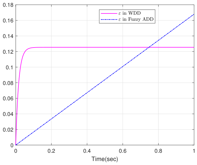
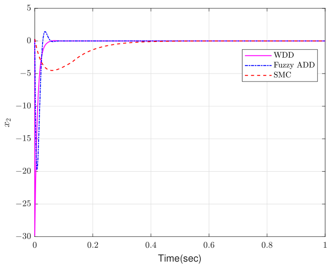
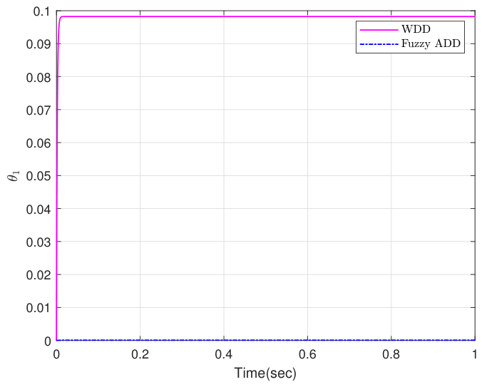
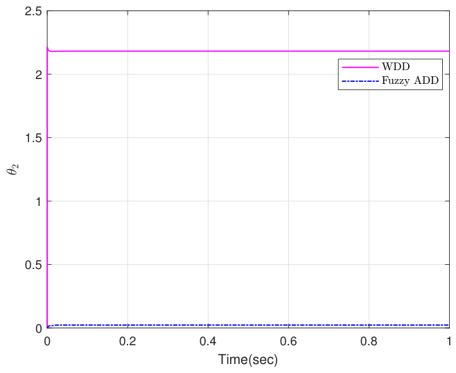
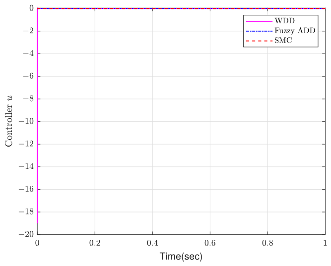
The simulation results are shown in Figure 1, Figure 2, Figure 3, Figure 4, Figure 5 and Figure 6. Figure 1 and Figure 2 compare the state trajectories x 1 and x 2 under the WDD, Fuzzy ADD, and SMC controllers. The WDD and Fuzzy ADD controllers drive both states close to zero within a short transient, whereas the SMC controller exhibits a slower convergence rate and a larger residual tracking error. Figure 3 and Figure 4 show the adaptive estimates θ 1 and θ 2 for the WDD and Fuzzy ADD controllers; the SMC controller is not included in these two figures because it does not use adaptive parameter estimation. Figure 5 compares the control inputs of the three controllers. The WDD controller generates a relatively large initial input because conservative lower and upper bounds are used in the WDD design, whereas the Fuzzy ADD and SMC controllers require smaller control inputs. Figure 6 shows the evolution of the residual-related term ε . For the proposed WDD controller, ε remains bounded because it is generated by the integrable function α ( t ) . In contrast, the corresponding term in the Fuzzy ADD design increases with time because the derivative of its Lyapunov function contains a positive constant residual.
To provide a more balanced comparison, Table 1 reports both tracking/attenuation performance and control effort over T = 1 s. The tracking and attenuation indexes include ISE x 1 , IAE x 1 , ITAE x 1 , the estimated L 2 -gain index γ ^ L 2 , and the settling time t s . The control-effort indexes include the peak input u peak , the RMS input u rms , and the control energy E u = 0 T u 2 ( t ) d t .
According to Table 1, the proposed WDD controller achieves the smallest ISE x 1 and the smallest estimated L 2 -gain index, which indicates better tracking accuracy and disturbance attenuation in this example. The Fuzzy ADD controller also achieves fast convergence and uses a much smaller input than WDD. The SMC controller requires the lowest control effort, but its tracking indexes and settling time are considerably larger than those of WDD and Fuzzy ADD. These results show a clear trade-off: WDD improves tracking and attenuation performance at the expense of a larger transient control input, whereas SMC reduces the input magnitude but sacrifices tracking performance.
Simulation 4: To further investigate the sensitivity of the proposed WDD controller with respect to the unknown virtual control coefficients, six simulation tests are conducted and the test results are shown in Table 2, which contains the tracking performance, attenuation index, settling time, and control effort for several representative values of ρ . It can be observed that the tracking performance in all tested cases is satisfactory. As ρ increases, the tracking indices slightly decrease, whereas the peak value, RMS value, and energy of the control input increase significantly, especially near ρ = 0.96 . These results show that the proposed WDD controller can preserve closed-loop stability under large variations of the unknown virtual control coefficients, at the cost of a larger transient control effort.
Remark 6.
The integrable function α ( t ) plays a key role in the proposed WDD controller. Since 0 α ( t ) d t is finite, the residual term in the WDD inequality remains bounded after integration. In contrast, the Fuzzy ADD design in [27] uses fuzzy universal approximators and Young’s inequality to deal with the approximation error; therefore, the derivative of the Lyapunov function contains a positive constant residual, whose integral becomes unbounded over an infinite time interval. Compared with the Fuzzy ADD and traditional SMC benchmarks, the WDD controller is more conservative because the virtual control coefficients are estimated by their lower bounds and the other uncertainties are estimated by their upper bounds. This conservatism explains the larger transient control input observed in Figure 5 and Table 1. However, it also leads to the improved tracking and disturbance-attenuation indexes reported in Table 1.

4.2. Example 2 (Experiments on the Real System)

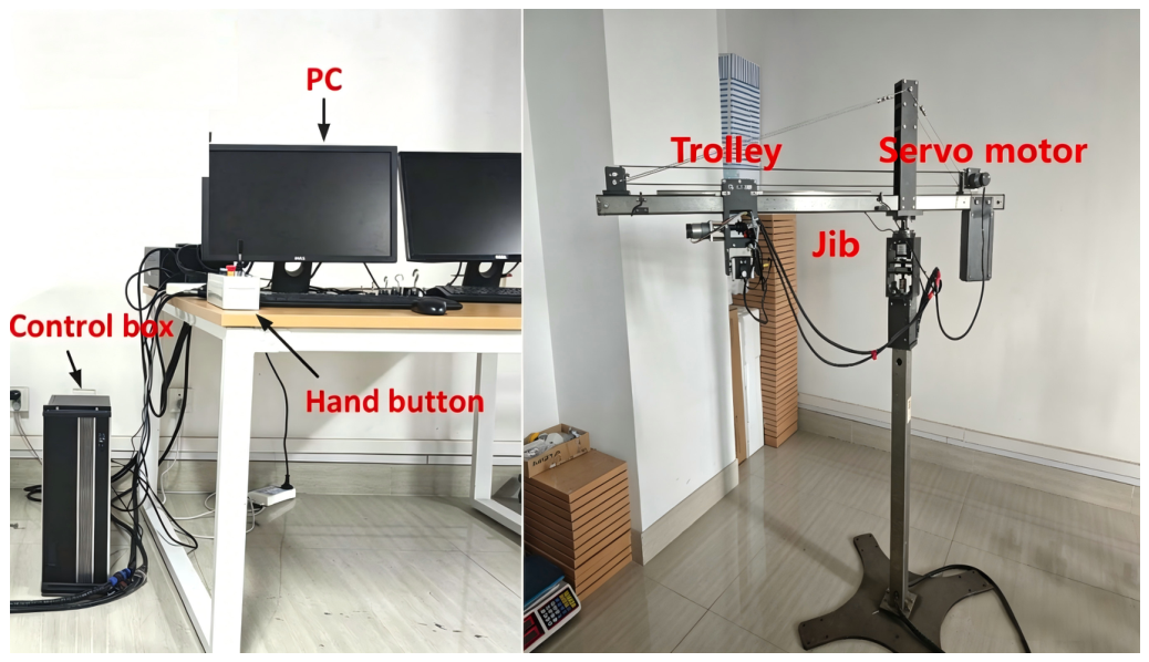
As illustrated in Figure 7, a single-link robot manipulator model is considered to evaluate the effectiveness of the proposed WDD method. The system dynamics can be described as
M t ϰ ¨ = u D ϰ ˙ + q
where ϰ denotes the angular position of the rotating arm and ϰ ˙ represents the angular velocity. The control input is denoted by u. The parameter D is an unknown friction coefficient 0 < D < D ¯ , while q represents an external disturbance. The physical parameters of the single-link robot manipulator are listed in Table 3.
By introducing the state variables x 1 = ϰ and x 2 = ϰ ˙ , and defining g 1 = 1 , f 1 = 0 , s 1 = 0 , g 2 = 1 M η e 2 + J , f 2 u = D M η e 2 + J ϰ ˙ , and s 2 = 1 M η e 2 + J , Equation (61) can be rewritten in the form of (1). It can be verified that Assumptions 1–2 are satisfied with g ̲ 1 = g ¯ 1 = g 1 , g ̲ 2 = g ¯ 2 = g 2 , g ̲ 1 k = g ¯ 1 k = g ̲ 2 k = g ¯ 2 k = 1 , and ϕ 2 u p = D ¯ M η e 2 + J , ϕ 2 k p = ϰ ˙ . The equilibrium points of the system is given by z 1 = 0 and z 2 = 0 . Let the desired output be y d = 0 . Under linearization, the closed-loop system can be written as
z ˙ 1 z ˙ 2 = A z 1 z 2
where A = k 1 1 1 k 2 . The corresponding characteristic polynomial of the closed-loop system is
s I A = s 2 + k 1 + k 2 s + k 1 k 2 + 1
Let o 1 and o 2 be the desired poles. The desired characteristic polynomial is
s + o 1 s + o 2 = s 2 + o 1 + o 2 s + o 1 o 2
By matching the coefficients of Equations (62) and (63), the controller parameters k 1 and k 2 can be determined as
k 2 = p 1 + p 2 + p 1 + p 2 2 4 μ e o 1 o 2 1 2 k 1 = p 1 + p 2 + p 1 + p 2 2 4 o 1 o 2 1 2 + o 1 + o 2
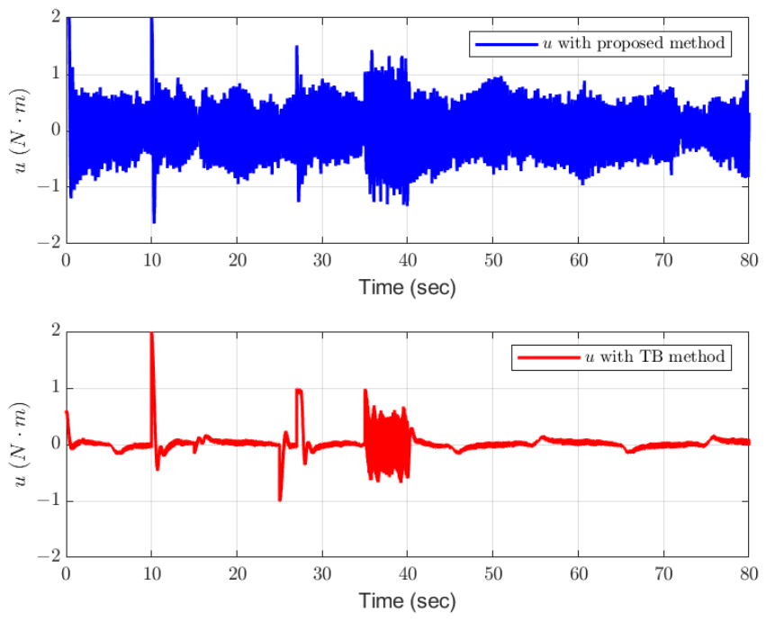
The settling time is selected as t s = 4 . Accordingly, the desired poles are chosen as o 1 = 4 t s = 1 and o 2 = 5 . Therefore, the control parameters are obtained as k 1 = 0.7639 and k 2 = 5.2361 . The initial conditions are set as x 1 0 , x 2 0 , θ 2 0 T = 0 7 × 1 . In addition, the parameters are chosen as v 1 = v 2 = 0 , h 1 = 0 , h 2 = 1 , and α 1 = α 2 = α 1 f = α 1 g = α 2 f = α 2 g = 1 e 0.01 t . The disturbance signal q is defined as
q = e 0.5 t 10 , if 10 < t < 15 s 1 , if 25 < t < 26 s r a n d 1 , 1 , if 35 < t < 40 s 0 , otherwise
For comparison, a traditional backstepping (TB) controller is also implemented on the same experimental platform. The TB controller is selected as the baseline because the single-link manipulator can be written as a second-order strict-feedback system.
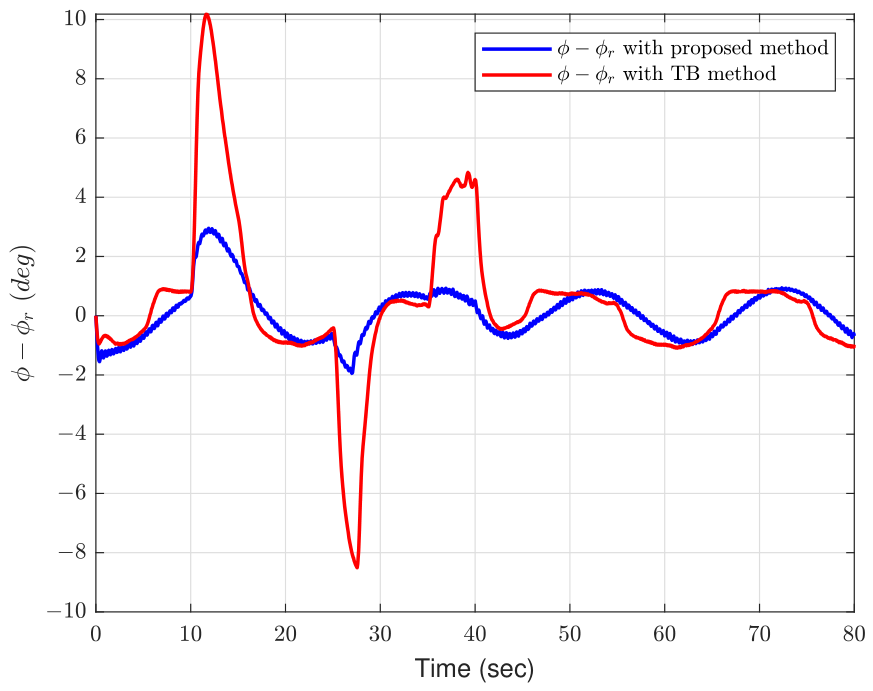
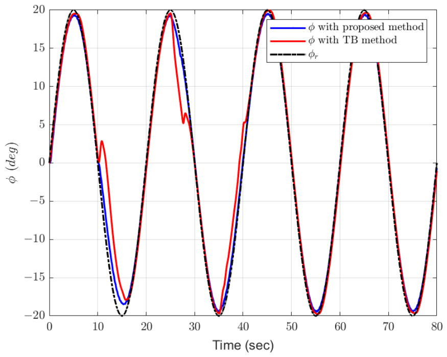
In Figure 8, Figure 9 and Figure 10, it can be observed that the steady-state value of ϕ obtained by the proposed approach is closer to zero than that of the TB method. Moreover, the proposed approach exhibits stronger disturbance attenuation capability when subjected to disturbance (Equation (64)). The experiment results fully demonstrate the effectiveness of the proposed WDD control scheme.

5. Conclusions

In this article, a novel concept called WDD has been defined. By constructing Lyapunov functions and using inequalities, a WDD controller for uncertain strict feedback-like systems was designed. Furthermore, with the proposed control scheme, the WDD problem for uncertain strict feedback-like systems was solved, and asymptotic convergence of the system states was achieved. Finally, an illustrative example was simulated. The stability analysis and simulations showed the effectiveness of the proposed controller. In the future, the prescribed-time control will be studied for uncertain strict-feedback systems with disturbances. This control strategy can also be extended to applications in bionic robotics and related fields, such as controlling the deformation of artificial external ears in bat-inspired robotic systems.

Author Contributions

Conceptualization, X.L.; methodology, X.L.; software, W.P.; validation, N.W.; writing—original draft preparation, G.D. and N.W.; writing—review and editing, G.D. and N.W. All authors have read and agreed to the published version of the manuscript.

Funding

This research was funded by the National Natural Science Foundation of China (62173127, 62472143), Key R&D Special Projects in Henan Province (241111521000), Program for Scientific and Technological Innovation Team in Universities of Henan Province (25IRTSTHN021), Top Young Talents in Central Plains ((2023)11), Cultivation Project of Tuoxin Team in Henan University of Technology (2024TXTD17), and Henan University of Technology High-Level Talent Fund (2024BS093).

Institutional Review Board Statement

Not applicable.

Informed Consent Statement

Not applicable.

Data Availability Statement

The simulation data supporting the findings of this study (including system state trajectories, control input sequences, and parameter configurations) are publicly available on Zenodo at https://doi.org/10.5281/zenodo.18245648.

Acknowledgments

The authors acknowledge Cunggen Liu and Jingyu Li for their assistance in this research. With their help, we completed this research together.

Conflicts of Interest

The authors declare no conflicts of interest.

References

  1. Guo, L.; Chen, W.H. Disturbance attenuation and rejection for systems with nonlinearity via DOBC approach. Int. J. Robust. Nonlinear Control 2005, 15, 109–125. [Google Scholar] [CrossRef] [Scilit]
  2. Ji, Y.; Huang, X.; Niu, B.; Li, Y.; Zhao, X.; Song, G. Prescribed-time tracking control for nonlinear systems: A nonvanishing disturbance observer-based approach. IEEE Trans. Syst. Man Cybern. Syst. 2026, 1–10. [Google Scholar] [CrossRef] [Scilit]
  3. Zheng, Q.; Dong, L.; Lee, D.H.; Gao, Z. Active disturbance rejection control for MEMS gyroscopes. IEEE Trans. Control Syst. Technol. 2009, 17, 1432–1438. [Google Scholar] [CrossRef] [Scilit]
  4. Wang, H.; Meng, Y.; Sun, J.; Zhang, L.; Zhang, H.; Zheng, S. Dual-coil active disturbance rejection control for compact MEG measurement systems. Control Eng. Pract. 2026, 170, 106833. [Google Scholar] [CrossRef] [Scilit]
  5. Chen, Y.; Han, B.; Tian, P.; Shangguan, S.; Li, Y.; Feng, R. Adaptive active disturbance rejection control for suppressing multiple uncertain periodic magnetic field disturbances. IEEE Trans. Ind. Electron. 2026, 1–13. [Google Scholar] [CrossRef] [Scilit]
  6. Willems, J.C.; Commault, C. Disturbance decoupling by measurement feedback with stability or pole placement. SIAM J. Control Optim. 1981, 19, 490–504. [Google Scholar] [CrossRef] [Scilit]
  7. Marro, G. Controlled; Conditioned Invariants in Linear System Theory; Prentice Hall: Hoboken, NJ, USA, 1992. [Google Scholar]
  8. Willems, J.C. Almost invariant subspaces: An approach to high gain feedback design–Part I: Almost controlled invariant subspaces. IEEE Trans. Autom. Control 1981, 26, 235–252. [Google Scholar] [CrossRef] [Scilit]
  9. Marino, R.; Respondek, W.; Van der Schaft, A.J. Almost disturbance decoupling for single-input single-output nonlinear systems. IEEE Trans. Autom. Control. 1989, 34, 1013–1017. [Google Scholar] [CrossRef] [Scilit]
  10. Liu, X.P.; Jutan, A.; Jutan, S. Almost disturbance decoupling of MIMO nonlinear systems and application to chemical processes. Automatica 2004, 40, 465–471. [Google Scholar] [CrossRef] [Scilit]
  11. Isidori, A.; Astolfi, A. Disturbance attenuation and H-control via measurement feedback in nonlinear systems. IEEE Trans. Autom. Control 1992, 37, 1283–1293. [Google Scholar] [CrossRef] [Scilit]
  12. Weiland, S.; Willemsc, J.C. Almost disturbance decoupling with internal stability. IEEE Trans. Autom. Control 1989, 34, 277–286. [Google Scholar] [CrossRef] [Scilit]
  13. Lin, Z. H almost disturbance decoupling with internal stability for linear systems subject to input saturation. IEEE Trans. Autom. Control 1997, 42, 992–995. [Google Scholar]
  14. Zou, R.M.; Malabre, M. Almost disturbance decoupling and pole placement. Automatica 2009, 45, 2685–2691. [Google Scholar] [CrossRef] [Scilit]
  15. Marino, R.; Tomei, P. Adaptive output feedback regulation with almost disturbance decoupling for nonlinearly parameterized systems. Int. J. Robust Nonlinear Control 2000, 10, 655–669. [Google Scholar] [CrossRef] [Scilit]
  16. Qian, C.J.; Wei, L. Almost disturbance decoupling for a class of high order nonlinear systems. IEEE Trans. Autom. Control 2000, 45, 1208–1214. [Google Scholar] [CrossRef] [Scilit]
  17. Chien, T.L.; Chen, C.C.; Huang, Y.C.; Lin, W.J. Stability and almost disturbance decoupling analysis of nonlinear system subject to feedback linearization and feedforward neural network controller. IEEE Trans. Neural Netw. 2008, 19, 1220–1230. [Google Scholar] [CrossRef] [Scilit]
  18. Li, C.Y.; Wang, W. Fuzzy almost disturbance decoupling for MIMO nonlinear uncertain systems based on high-gainobserver. Neurocomputing 2013, 111, 104–114. [Google Scholar] [CrossRef] [Scilit]
  19. Li, C.Y.; Zhong, J.H. Fuzzy output feedback control with almost disturbance decoupling for MIMO nonlinear systems. In Proceedings of the 33rd Chinese Control Conference; IEEE: New York, NY, USA, 2014; pp. 4514–4519. [Google Scholar]
  20. Marino, R.; Tomei, P. Nonlinear output feedback tracking with almost disturbance decoupling. IEEE Trans. Autom. 1999, 44, 18–28. [Google Scholar] [CrossRef] [Scilit]
  21. Chang, P.F.; Chen, C.C.; Chang, J.R. Observer-based feedback linearizatiorcontrol of multi-input multi-outputnonlinear system and application todouble rotor system. Adv. Mech. Eng. 2019, 11, 1–14. [Google Scholar] [CrossRef] [Scilit]
  22. Chu, H.; Qian, C.; Yang, J. Almost disturbance decoupling for a class of nonlinear systems via sampled-data output feedback control. Int. J. Robust Nonlinear Control 2016, 26, 2201–2215. [Google Scholar] [CrossRef] [Scilit]
  23. Sun, Z.Y.; Zhang, C.H.; Wang, Z. Adaptive disturbance attenuation for generalized high-order uncertain nonlinear systems. Automatica 2017, 80, 102–109. [Google Scholar] [CrossRef] [Scilit]
  24. Meng, Q.H.; Wang, P.; Sun, Z.Y.; Chen, C.C. Almost disturbance decoupling for a class of nonlinear systems subject to time-delays via sampled-data output feedback control. Asian J. Control 2018, 20, 568–576. [Google Scholar] [CrossRef] [Scilit]
  25. Jiang, K.; Wang, X.M.; Niu, B. Finite-time adaptive neural control and almost disturbance decoupling for disturbed MIMO non-strict-feedback nonlinear systems. J. Frankl. Inst. 2020, 357, 11750–11772. [Google Scholar] [CrossRef] [Scilit]
  26. Wang, X.H.; Chen, Q.L. Fixed-time stabilisation with almost disturbance decoupling for nonlinear systems under p-normal form. Int. J. Control 2024, 97, 2987–2996. [Google Scholar] [CrossRef] [Scilit]
  27. Chen, B.; Tong, S.C.; Liu, X.P. Fuzzy approximate disturbance decoupling of MIMO nonlinear systems by backstepping approach. Fuzzy Sets Syst. 2007, 158, 1097–1125. [Google Scholar] [CrossRef] [Scilit]
  28. Wang, N.; Liu, X.P.; Liu, C.G.; Wang, H.Q.; Li, J.Y. An almost disturbance decoupling control strategy for 4-DOF tower cranes. Mech. Syst. Signal Process. 2025, 224, 111927. [Google Scholar] [CrossRef] [Scilit]
  29. Liu, C.G.; Zhang, Z.W.; Liu, X.P.; Wang, H.Q.; Li, L.L.; Li, C.D. Nonlinear end-effector tracking control with almost disturbance decoupling for five-DOF tower cranes. IEEE Trans. Ind. Electron. 2026, 1–11. [Google Scholar] [CrossRef] [Scilit]
  30. Doruk, R.Ö.; Kocaoglan, E. An almost disturbance decoupling solution of the attitude control problem. Aircr. Eng. Aerosp. Technol. 2008, 80, 295–307. [Google Scholar] [CrossRef] [Scilit]
  31. Chien, T.L.; Chen, C.C.; Tsai, M.C. Almost disturbance decoupling and tracking control for multi-input multi-output non-linear uncertain systems: Application to a half-car active suspension system. Proc. Inst. Mech. Eng. 2009, 223, 215–228. [Google Scholar] [CrossRef] [Scilit]
  32. Zhong, Z.Z.; Wang, J.C. Looper-tension almost disturbance decoupling control for hot strip finishing mill based on feedback linearization. IEEE Trans. Ind. Electron. 2010, 58, 3668–3679. [Google Scholar] [CrossRef] [Scilit]
  33. Chen, C.C.; Lin, Y.F.; Chen, M.H. Nonlinear tracking with almost disturbance decoupling and its application to ball and beam system. J. Chin. Inst. Eng. 2007, 30, 545–551. [Google Scholar] [CrossRef] [Scilit]
  34. Kang, S.; Nagamune, R.; Yan, H. Almost disturbance decoupling force control for the electro-hydraulic load simulator with mechanical backlash. Mech. Syst. Signal Process. 2020, 135, 106400. [Google Scholar] [CrossRef] [Scilit]
  35. Li, Y.X.; Tong, S.C. A bound estimation approach for adaptive fuzzy asymptotic tracking of uncertain stochastic nonlinear systems. IEEE Trans. Cybern. 2020, 52, 5333–5342. [Google Scholar] [CrossRef] [Scilit] [PubMed]
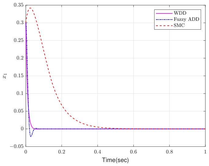
Figure 1. State response x 1 under the WDD, Fuzzy ADD, and SMC controllers.
Actuators 15 00325 g001
Figure 2. State response x 2 under the WDD, Fuzzy ADD, and SMC controllers.
Actuators 15 00325 g002
Figure 3. Adaptive parameter estimate θ 1 of the WDD and Fuzzy ADD controllers.
Actuators 15 00325 g003
Figure 4. Adaptive parameter estimate θ 2 of the WDD and Fuzzy ADD controllers.
Actuators 15 00325 g004
Figure 5. Control input u under the WDD, Fuzzy ADD, and SMC controllers.
Actuators 15 00325 g005
Figure 6. Evolution of the residual-related term ε for the WDD and Fuzzy ADD controllers.
Actuators 15 00325 g006
Figure 7. The single-link robot manipulator.
Actuators 15 00325 g007
Figure 8. The state ϕ under the WDD and TB controllers.
Actuators 15 00325 g008
Figure 9. The tracking error ϕ - y d ϕ under the WDD and TB controllers.
Actuators 15 00325 g009
Figure 10. The controller τ ϕ under the WDD and TB controllers.
Actuators 15 00325 g010
Table 1. Quantitative comparison of tracking performance and control effort computed from the simulation trajectories ( T = 1 s).
ControllerTracking and Attenuation PerformanceControl Effort
ISE x 1 IAE x 1 ITAE x 1 γ ^ L 2 t s (s) u peak u rms E u = 0 T u 2 ( t ) dt
WDD 4.16 × 10 4 2.74 × 10 3 2.49 × 10 5 2.69 × 10 3 1.41 × 10 1 1.90 × 10 6 4.06 × 10 3 1.65 × 10 7
Fuzzy ADD 7.13 × 10 4 3.52 × 10 3 3.10 × 10 5 3.52 × 10 3 1.13 × 10 1 3.06 × 10 3 1.65 × 10 2 2.72 × 10 4
Traditional SMC 1.13 × 10 2 4.85 × 10 2 4.71 × 10 3 1.40 × 10 2 7.19 × 10 1 1.21 × 10 2 1.54 × 10 1 2.36 × 10 2
Note: ISE x 1 = 0 T x 1 2 ( t ) dt , IAE x 1 = 0 T x 1 ( t ) dt , ITAE x 1 = 0 T x 1 ( t ) dt , and γ ^ L 2 = 0 T x 1 2 ( t ) dt / 0 T q 2 ( t ) dt . The settling time ts is computed using the threshold 10−3 with a continuous time window of 0.05 s.
Table 2. Sensitivity analysis of the proposed WDD controller with respect to ρ under variations of the virtual control coefficients ( T = 1 s).
ρ Coefficient RangesStableTracking and Attenuation PerformanceControl Effort
g 1 ρ ( t ) g 2 ρ ( t ) ISE x 1 IAE x 1 ITAE x 1 γ ^ L 2 t s (s) u peak u rms E u = 0 T u 2 ( t ) dt
0.00 [ 1.00 , 1.00 ] [ 2.00 , 2.00 ] Yes 5.10 × 10 4 3.37 × 10 3 3.73 × 10 5 2.98 × 10 3 1.72 × 10 1 1.44 × 10 6 3.31 × 10 3 1.09 × 10 7
0.20 [ 0.80 , 1.20 ] [ 1.60 , 2.40 ] Yes 4.16 × 10 4 2.74 × 10 3 2.49 × 10 5 2.69 × 10 3 1.38 × 10 1 1.90 × 10 6 3.80 × 10 3 1.44 × 10 7
0.40 [ 0.60 , 1.40 ] [ 1.20 , 2.80 ] Yes 3.51 × 10 4 2.32 × 10 3 1.76 × 10 5 2.47 × 10 3 9.56 × 10 2 2.79 × 10 6 4.60 × 10 3 2.12 × 10 7
0.60 [ 0.40 , 1.60 ] [ 0.80 , 3.20 ] Yes 3.04 × 10 4 2.00 × 10 3 1.30 × 10 5 2.30 × 10 3 7.66 × 10 2 5.15 × 10 6 6.25 × 10 3 3.91 × 10 7
0.80 [ 0.20 , 1.80 ] [ 0.40 , 3.60 ] Yes 2.68 × 10 4 1.77 × 10 3 1.01 × 10 5 2.16 × 10 3 5.13 × 10 2 1.73 × 10 7 1.15 × 10 4 1.31 × 10 8
0.96 [ 0.04 , 1.96 ] [ 0.08 , 3.92 ] Yes 2.44 × 10 4 1.63 × 10 3 8.73 × 10 6 2.06 × 10 3 5.35 × 10 2 4.03 × 10 8 5.53 × 10 4 3.06 × 10 9
Note: ISE x 1 = 0 T x 1 2 ( t ) dt , IAE x 1 = 0 T x 1 ( t ) dt , ITAE x 1 = 0 T x 1 ( t ) dt , and γ ^ L 2 = 0 T x 1 2 ( t ) dt / 0 T q 2 ( t ) dt . The coefficient ranges are obtained from g 1 ρ ( t ) = 1 + ρ cos ( 0.2 π t ) and g 2 ρ ( t ) = 2 + 2 ρ sin ( 0.2 π t ) . “Stable” means that x 1 ( t ) and x 2 ( t ) remain below 10−3 for a continuous time window of 0.05 s.
Table 3. Physical parameters of the single-link robot manipulator.
ParameterSymbolValue
Mass of the loadM 1.852 kg
Inertia moment of the rotating armJ 1.532 kg·m2
Distance from the load to the rotation center η e 0.17 m
Equivalent inertia M t = M η e 2 + J 1.5855 kg·m2
Friction coefficientDUnknown, 0 < D < D ¯
Disclaimer/Publisher’s Note: The statements, opinions and data contained in all publications are solely those of the individual author(s) and contributor(s) and not of MDPI and/or the editor(s). MDPI and/or the editor(s) disclaim responsibility for any injury to people or property resulting from any ideas, methods, instructions or products referred to in the content.