Active Disturbance Rejection Control of Quadrotor UAVs Under Uncertainties and Disturbances

Abstract

Quadrotor unmanned aerial vehicles (UAVs), commonly known as quadcopters, pose a fundamental control challenge: they are underactuated, open-loop unstable, strongly coupled across six degrees of freedom, and highly susceptible to aerodynamic disturbances and payload uncertainty. Classical model-based controllers degrade significantly when the vehicle mass shifts due to battery discharge or payload pickup, or when wind gusts produce forces comparable to the available thrust margin—an especially acute problem for nano-scale quadcopters. This paper proposes an active disturbance rejection control (ADRC) to address these challenges. Rather than attempting to model every source of uncertainty, we employ an extended state observer (ESO) to estimate a single total disturbance signal—comprising unmodeled dynamics, parametric errors, nonlinear coupling, and external disturbances—in real time from sensor measurements alone, and cancel it before applying a simple feedback law. Building on this principle, we derive a cascaded linear ADRC (LADRC) architecture that governs all six degrees of freedom of the quadcopter and formulate the quadrotor-specific total-disturbance structure for each control channel. Simulations demonstrate that the proposed controller maintains small, bounded position-tracking RMS errors under 30% mass uncertainty combined with a sustained lateral wind-gust disturbance, while delivering the correct hover thrust automatically without prior knowledge of the true mass and without integrator wind-up.

1. Introduction

Quadrotor UAVs, commonly known as quadcopters, have become a canonical platform for autonomous flight research owing to their mechanical simplicity, hovering capability, and agility. However, these same properties give rise to a demanding control problem. A quadcopter has four independently actuated rotors but six degrees of freedom, rendering it underactuated: lateral motion can be achieved only by tilting the vehicle, which couples translational and rotational dynamics. The open-loop system is unstable, and its dynamics are highly nonlinear and subject to three categories of disturbances that resist precise modelling: (1) Aerodynamic effects. Blade flapping, induced drag, ground effect, rotor-to-rotor wake interaction, and wind gusts all produce forces and torques that depend on airspeed, rotor speed, and proximity to obstacles in a complex, hard-to-model manner. (2) Parametric uncertainty. The vehicle mass varies as the battery discharges or when a payload is attached, and the thrust and torque coefficients change with rotor speed and air density. (3) Unmodeled dynamics. Flexible structures, the combined electrical and mechanical lag, propeller gyroscopic effects, and battery-voltage sag introduce internal dynamics that are typically neglected in the nominal model. These challenges are amplified for nano-scale quadcopters such as the Crazyflie [1] ($m=27$ g, 10 cm wheelbase): the thrust-to-weight margin is modest, and a lateral wind force of just 30 mN—roughly 11% of hover thrust—produces perceptible trajectory deviation.

The most common flight controller for quadcopters is a cascaded proportional-integral-derivative (PID) controller, used, for example, in the official Crazyflie firmware [1]. PID controllers are intuitive to tune and computationally cheap, but they handle disturbances reactively through integral action, which leads to wind-up, slow rejection, and sensitivity to gain mismatch when plant parameters change. Model-based alternatives such as $H_{\infty }$ synthesis [2] and model-predictive control (MPC) [3] offer stronger guarantees but require an accurate linear or nonlinear model and involve solving optimization problems that may be too computationally expensive for a microcontroller running at 1 kHz. Feedback linearization is sensitive to modeling errors in the linearizing terms, since any mismatch propagates directly into the invese dynamics. Sliding-mode control (SMC) [4,5], by contrast, is intrinsically robust to matched uncertainty and can be designed with boundary-layer or higher-order sliding modes [6] to mitigate the chattering associated with the classical first-order discontinuous law; nevertheless, the selection of the sliding surface, the boundary-layer thickness, and the switching gain may require bounds on the uncertainty that may not be available a priori on a nano-quadcopter. Adaptive control and ${\mathcal{L}}_1$ adaptive control [7,8,9] update an online model of the plant and offer good transient performance, but their adaptation laws require persistent excitation, careful stability analysis for each configuration, and substantial parameterization effort. Recent learning-based approaches—including online reinforcement learning and deep model-reference adaptive control directly from input–output data [10,11]—can adapt to faulty actuation and uncertain dynamics without an explicit plant model and embed stability guarantees by construction; their main practical limitations on a nano-platform are the on-board memory and computation required for neural-network inference, and the need for asynchronous task scheduling between the learning loop and the control loop. The proposed ADRC retains the model-free spirit of learning-based control while keeping the on-board computation restricted to a single linear observer per channel, which is what makes it a natural fit for the Crazyflie’s onboard microcontroller.

Active disturbance rejection control (ADRC), introduced by Han [12] and later cast in linear form with a transparent bandwidth-based tuning procedure by Gao [13], takes a fundamentally different view of the control problem. ADRC has been successfully applied across a range of domains, from industrial process control [13] to quadrotor tracking control [14]. Rather than constructing a high-fidelity plant model and inverting it, ADRC treats every effect not captured by a chosen low-order canonical form— unmodeled dynamics, parametric error, nonlinear coupling, and external disturbances—as a single total disturbance signal acting on each control channel. An extended state observer (ESO) estimates this signal online from input–output measurements alone, and the controller cancels it in a feed-forward fashion before a simple low-order feedback law acts on the resulting near-integrator residual.

In this paper, we propose an ADRC-based flight control approach for quadcopters operating in regimes where accurate aerodynamic models are unavailable, on-board computational budget is limited, and robust disturbance rejection—rather than asymptotic regulation under nominal conditions—is the dominant performance requirement. Although linear and nonlinear ADRC variants have previously been applied to quadrotors (see, e.g., [14] for a generalized PI-observer-based ADRC for trajectory tracking, and the references therein), the present paper differs from prior work in three concrete aspects:

(C1)

Per-channel total-disturbance decomposition. For each of the six control axes ($x,y,z,\varphi ,\theta ,\psi$), we derive an explicit analytical decomposition of the total disturbance $a_i\left(t\right)$ into a parametric term arising from mass or inertia mismatch through the input-gain residual $(b-b_0)u$, a nonlinear coupling term (gyroscopic for rotational channels, trigonometric tilt residual for translational channels), and an external term collecting aerodynamic forces/torques (Equations (27)–(32)). Unlike [14] and earlier ADRC quadrotor designs that treat the disturbance as a generic lumped signal, this decomposition allows to predict, before any experiment, which physical effects each ESO will absorb and how.

(C2)

Quantitative ESO error bound linked to a single bandwidth. We provide an explicit ultimate bound (Lemma 1) of order $\mathcal{O}(M/{\omega }_o)$ on the LESO estimation error and a closed-loop tracking bound (Theorems 1 and 2) that vanishes as ${\omega }_o\to \infty$, together with a separation-principle analysis for the cascaded position/attitude architecture that has not, to our knowledge, been spelled out for the LADRC quadrotor case.

(C3)

Combined mass-uncertainty/wind-gust validation on a nano-platform. We instantiate the design on the 27 g Crazyflie—a platform whose thrust margin makes it unusually sensitive to the disturbances considered—and demonstrate, in full nonlinear simulation, simultaneous rejection of $30\%$ mass uncertainty and a sustained 30 mN lateral wind gust without re-tuning, gain scheduling, or integrator action. We further verify that the resulting rotor commands remain within the physical RPM saturation limit. To the best of our knowledge, the combination of these two disturbance classes on a nano-quadcopter has not been reported in the prior ADRC literature.

In addition, we demonstrate that the ESO’s third state $z_3$ provides a real-time, physically interpretable estimate of the total disturbance, opening a pathway to in-flight fault detection and graceful degradation—a capability absent from standard PID flight controllers.

Throughout the paper, scalars are unbolded ($x\in \mathbb{R}$), vectors are bold lowercase ($\mathbf{x}\in {\mathbb{R}}^n$), and matrices are bold or italic uppercase. $\parallel \mathbf{x}\parallel$ denotes the Euclidean (${\mathsf{\ell }}_2$) norm of a vector and the induced ${\mathsf{\ell }}_2$ norm when applied to a matrix. ${\mathbf{x}}^{\top }$ denotes transpose, $A\succ 0$ means symmetric positive definite, and I denotes the identity matrix of the appropriate dimension. For a signal $v\left(t\right)$, ${\parallel v\parallel }_{\infty }={sup}_{t\ge 0}\left|v\left(t\right)\right|$. The notations $\dot{(·)}$, $\ddot{(·)}$, and ${(·)}^{\left(n\right)}$ denote the first, second, and n-th time derivative, respectively. The hat $\widehat{x}$ denotes an estimate of x; the tilde $\tilde{x}=\widehat{x}-x$ denotes the associated estimation error.

The remainder of this paper is organized as follows. Section 2 formulates the quadcopter control problem and derives the Crazyflie dynamic model. Section 3 develops the cascaded ADRC design, including LESO stability analysis and the per-channel total-disturbance formulation. Section 4 presents simulation results, and Section 5 concludes.

2. Problem Formulation

2.1. Quadcopter Dynamic Model

We consider the Crazyflie nano-quadcopter [1], whose physical parameters are listed in

Table 1. Crazyflie 2.1 physical parameters [1].

Symbol	Quantity	Value	Unit
m	Total mass	$0.027$	kg
L	Arm length	$0.046$	m
$I_{xx}$	Roll inertia	$1.657\times {10}^{-5}$	kg m2
$I_{yy}$	Pitch inertia	$1.657\times {10}^{-5}$	kg m2
$I_{zz}$	Yaw inertia	$2.9\times {10}^{-5}$	kg m2
$k_f$	Thrust coefficient	$3.16\times {10}^{-10}$	N/(r/min)2
$k_m$	Torque coefficient	$7.94\times {10}^{-12}$	N m/(r/min)2
g	Gravitational accel.	$9.81$	m/s2

.

Let $\mathcal{I}$ denote the inertial frame and $\mathcal{B}$ the body frame. Following the standard rigid-body modelling [15], the quadcopter position is $\mathbf{p}={[x,y,z]}^{\top }$, and its attitude is parameterized by the ZYX Euler angles $\mathit{\eta }={[\varphi ,\theta ,\psi ]}^{\top }$ (roll, pitch, yaw). Each rotor spinning at angular speed ${\Omega }_i$ produces a thrust $T_i=k_f{\Omega }_i^2$, giving a total thrust $F_T={\sum }_{i=1}^4{T}_i$. The translational dynamics are

$$m\ddot{\mathbf{p}}=F_T\mathbf{R}\left(\mathit{\eta }\right){\mathbf{e}}_3-mg{\mathbf{e}}_3+{\mathbf{d}}_p,$$

(1)

$$\ddot{x}=U_1(cos\psi sin\theta cos\varphi +sin\psi sin\varphi )+d_x/m,$$

(2)

$$\ddot{y}=U_1(sin\psi sin\theta cos\varphi -cos\psi sin\varphi )+d_y/m,$$

(3)

$$\ddot{z}=-g+U_{1}cos\varphi cos\theta +d_z/m,$$

(4)

where $\mathbf{R}\left(\mathit{\eta }\right)$ is the body-to-inertial rotation matrix, ${\mathbf{e}}_3={[0,0,1]}^{\top }$, $U_1=F_T/m$ is the mass-normalized thrust input, and ${\mathbf{d}}_p={[d_x,d_y,d_z]}^{\top }$ collects the aerodynamic force disturbances.

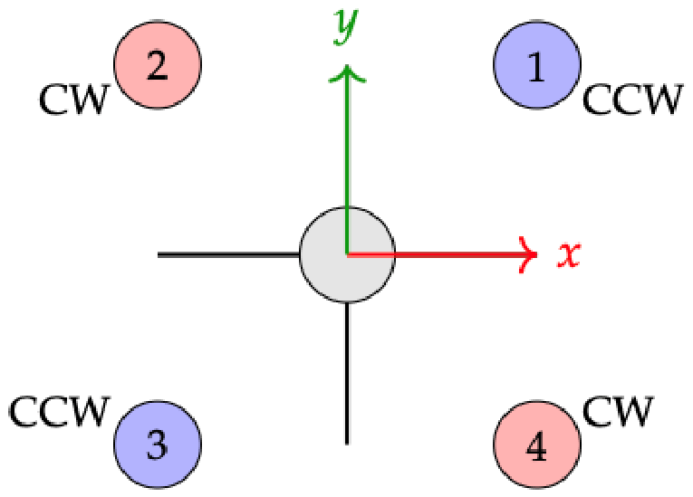
From the rotor arrangement in Figure 1, the body-frame control torques are

$${\tau }_{\varphi }=k_{f}L({\Omega }_4^2-{\Omega }_2^2),$$

(5)

$${\tau }_{\theta }=k_{f}L({\Omega }_3^2-{\Omega }_1^2),$$

(6)

$${\tau }_{\psi }=k_m({\Omega }_1^2-{\Omega }_2^2+{\Omega }_3^2-{\Omega }_4^2).$$

(7)

The rotational dynamics then follow from Euler’s equations as

$$\left(\begin{array}{ccc}{I}_{xx}& 0& 0\\ 0& I_{yy}& 0\\ 0& 0& I_{zz}\end{array}\right)\left(\begin{array}{c}\ddot{\varphi }\\ \ddot{\theta }\\ \ddot{\psi }\end{array}\right)=\left(\begin{array}{c}{U}_2\\ U_3\\ U_4\end{array}\right)+\left(\begin{array}{c}(I_{yy}-I_{zz})\dot{\theta }\dot{\psi }\\ (I_{zz}-I_{xx})\dot{\varphi }\dot{\psi }\\ (I_{xx}-I_{yy})\dot{\varphi }\dot{\theta }\end{array}\right)+\left(\begin{array}{c}{d}_{\varphi }\\ d_{\theta }\\ d_{\psi }\end{array}\right),$$

(8)

with $U_2={\tau }_{\varphi }$, $U_3={\tau }_{\theta }$, $U_4={\tau }_{\psi }$, and the gyroscopic coupling terms appearing explicitly. In the ADRC formulation of Section 3, these coupling terms will be absorbed into the per-channel total disturbance $a_i\left(t\right)$.

Given the virtual inputs ${[U_1,U_2,U_3,U_4]}^{\top }$, the squared rotor speeds are recovered through the control allocation

$$\left(\begin{array}{c}{\Omega }_1^2\\ {\Omega }_2^2\\ {\Omega }_3^2\\ {\Omega }_4^2\end{array}\right)={\left(\begin{array}{cccc}{k}_f& k_f& k_f& k_f\\ 0& -k_{f}L& 0& k_{f}L\\ -k_{f}L& 0& k_{f}L& 0\\ k_m& -k_m& k_m& -k_m\end{array}\right)}^{-1}\left(\begin{array}{c}{m}_{\mathrm{nom}}{U}_1\\ U_2\\ U_3\\ U_4\end{array}\right).$$

(9)

We emphasize that the allocation in (9) uses the nominal mass $m_{\mathrm{nom}}$, not the (unknown) true mass m. This is consistent with the ADRC principle: the on-board controller operates entirely on a priori parameters. Any residual error introduced by the allocation—arising from $\Delta m=m-m_{\mathrm{nom}}$, deviations of $k_f,k_m$ from their nominal values, or first-order motor–ESC delay—appears as an additional input-gain mismatch and is automatically absorbed into the total disturbance via the $(b-b_0)u$ term in (12). Consequently, no real-time knowledge of the true vehicle mass or thrust coefficients is required at any point in the control pipeline.

2.2. Control Objective

Let ${\mathbf{p}}_d\left(t\right)={[x_d\left(t\right),y_d\left(t\right),z_d\left(t\right)]}^{\top }$ be a smooth desired position trajectory and ${\psi }_d\left(t\right)$ a desired yaw angle. The control objective is to design a feedback law $\mathbf{u}\left(t\right)={[U_1,U_2,U_3,U_4]}^{\top }$ that maps on-board sensor measurements to rotor commands such that the closed-loop system satisfies

$$\underset{t\to \infty }{lim}\parallel \mathbf{p}\left(t\right)-{\mathbf{p}}_d\left(t\right)\parallel \le {ϵ}_p,$$

(10)

$$\underset{t\to \infty }{lim}|\psi \left(t\right)-{\psi }_d\left(t\right)|\le {ϵ}_{\psi },$$

(11)

for small ultimate bounds ${ϵ}_p,{ϵ}_{\psi }>0$, despite the three categories of disturbances enumerated in Section 1, and without requiring knowledge of their precise structure.

Table 2. Physical disturbance sources and their ADRC mapping.

Channel	Physical Sources	Absorbed into ${\mathit{a}}_{\mathit{i}\mathbf{\left(}\mathit{t}\mathbf{\right)}}$
z (altitude)	Gravity mismatch $(\Delta m)g$; drag $-k_d{v}_z$; battery-sag thrust loss	$a_z=-\Delta mg/m+\mathrm{drag}+\Delta b_{0,z}{U}_1$
$\varphi$ (roll)	Gyroscopic coupling; aerodynamic roll torque; inertia error $\Delta I_{xx}$	$a_{\varphi }=\Delta I_{xx}^{-1}{\tau }_{\varphi }+(I_{yy}-I_{zz})\dot{\theta }\dot{\psi }/I_{xx}$
$\theta$ (pitch)	Gyroscopic coupling; aerodynamic pitch torque; inertia error $\Delta I_{yy}$	$a_{\theta }=\Delta I_{yy}^{-1}{\tau }_{\theta }+(I_{zz}-I_{xx})\dot{\varphi }\dot{\psi }/I_{yy}$
$\psi$ (yaw)	Reaction torque imbalance; inertia error $\Delta I_{zz}$; motor–ESC delay	$a_{\psi }=\Delta I_{zz}^{-1}{\tau }_{\psi }+(I_{xx}-I_{yy})\dot{\varphi }\dot{\theta }/I_{zz}$
$x,y$ (position)	Wind force; nonlinear coupling at large tilt angles	$a_i=d_i/m+\mathrm{coupling}\mathrm{residual}$, $i\in \{x,y\}$

summarizes how the three physical disturbance categories manifest in each of the six control channels and how they are absorbed by the ADRC total disturbance $a_i\left(t\right)$, $i\in \{z,x,y,\varphi ,\theta ,\psi \}$, the formal construction of which is deferred to Section 3.

The central observation is that, regardless of which physical sources contribute, each channel’s total disturbance $a_i\left(t\right)$ is observable from the output of that channel through an ESO; no individual identification of aerodynamic coefficients, inertia errors, or wind parameters is required. The formal basis of this claim is that, once $a_i\left(t\right)$ is treated as an additional state $x_3$ of the augmented plant (15), the resulting triple $(A,B,C)$ in canonical observable form is trivially observable; the LESO in (17), whose error dynamics are characterized in Lemma 1, then reconstructs $a_i\left(t\right)$ with an $\mathcal{O}(1/{\omega }_o)$ ultimate bound. Section 3 develops both the augmentation and the bound in detail.

3. ADRC-Based Control Design for Quadcopters

3.1. Fundamentals of ADRC and Stability Analysis

ADRC casts a SISO control problem into a canonical integrator-chain form in which all model uncertainty and external disturbance is lumped into a single signal. For a channel of relative degree n with output y and input u, the dynamics are written as

$$y^{\left(n\right)}=\underset{{\displaystyle a\left(t\right)(\mathrm{total}\mathrm{disturbance})}}{\underbrace{f\left(y,\dot{y},\dots ,y^{(n-1)},d\left(t\right),t\right)+(b-b_0)u}}+b_{0}u,$$

(12)

where b is the unknown true input gain, $b_0$ is its rough nominal estimate (e.g., $1/I_{xx,\mathrm{nom}}$ for the roll channel), and $f(·)$ collects all internal nonlinearities together with the external disturbance $d\left(t\right)$. The lumped signal $a\left(t\right)$ is referred to as the total disturbance; crucially, $a\left(t\right)$ need not be modeled, only estimated.

If a real-time estimate $\widehat{a}\left(t\right)$ of the total disturbance is available, the control law

$$u={\displaystyle \frac{u_0-\widehat{a}\left(t\right)}{b_0}}$$

(13)

substituted into (12) yields

$$y^{\left(n\right)}=a\left(t\right)-\widehat{a}\left(t\right)+u_0\approx u_0,$$

(14)

i.e., the closed-loop plant becomes a pure integrator chain driven by $u_0$ as if no disturbance existed. The remaining task is to choose $u_0$ to stabilize this nominal chain and track the desired trajectory—a textbook pole-placement problem.

The estimate $\widehat{a}\left(t\right)$ can be produced by an extended state observer (ESO) that augments the plant state with $a\left(t\right)$ as an additional state. For the second-order case ($n=2$), which covers all six quadcopter channels, define $x_1=y$, $x_2=\dot{y}$, $x_3=a\left(t\right)$. The augmented system becomes

$$\dot{\mathbf{x}}=A\mathbf{x}+Bu+E\dot{a},y=C\mathbf{x},$$

(15)

with

$$A=\left(\begin{array}{ccc}0& 1& 0\\ 0& 0& 1\\ 0& 0& 0\end{array}\right),B=\left(\begin{array}{c}0\\ b_0\\ 0\end{array}\right),E=\left(\begin{array}{c}0\\ 0\\ 1\end{array}\right),C=\left(\begin{array}{ccc}1& 0& 0\end{array}\right).$$

(16)

Following the approach in [13,16], we adopt the linear ESO (LESO) and parameterize its three correction gains ${\beta }_1,{\beta }_2,{\beta }_3$ by a single observer bandwidth ${\omega }_o$:

$$\left\{\begin{array}{c}{\dot{z}}_1=z_2-{\beta }_1(z_1-y),\hfill \\ {\dot{z}}_2=z_3-{\beta }_2(z_1-y)+b_{0}u,\hfill \\ {\dot{z}}_3=-{\beta }_3(z_1-y),\hfill \end{array}\right.\begin{array}{cc}\hfill {\beta }_1& =3{\omega }_o,\hfill \\ \hfill {\beta }_2& =3{\omega }_o^2,\hfill \\ \hfill {\beta }_3& ={\omega }_o^3.\hfill \end{array}$$

(17)

where $z_1,z_2,z_3$ are the estimates of $x_1,x_2,x_3$, respectively. This choice places all three observer eigenvalues at $-{\omega }_o$, reducing the design effort to a single tuning parameter with clear physical meaning.

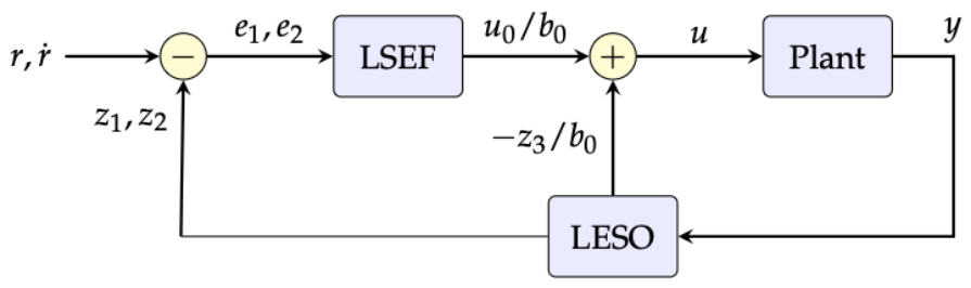
With the LESO providing $z_1\approx y$, $z_2\approx \dot{y}$, and $z_3\approx a\left(t\right)$, the inner feedback $u_0$ is taken as a PD law parameterized by a single controller bandwidth ${\omega }_c$ (the LSEF block in Figure 2):

$$u_0=k_p(r-z_1)+k_d(\dot{r}-z_2),k_p={\omega }_c^2,k_d=2{\omega }_c,$$

(18)

where r and $\dot{r}$ are the reference position and velocity. The total control signal is then

$$u={\displaystyle \frac{u_0-z_3}{b_0}}.$$

(19)

A block diagram of the resulting LADRC is shown in Figure 2.

In what follows, we establish the boundedness of both the observer error and the closed-loop tracking error. Let $\tilde{\mathbf{z}}=\mathbf{z}-\mathbf{x}={[{\tilde{z}}_1,{\tilde{z}}_2,{\tilde{z}}_3]}^{\top }$ denote the LESO estimation error, where $\mathbf{z}={[z_1,z_2,z_3]}^{\top }$. It follows from (15) and (17) that the error dynamics are

$$\dot{\tilde{\mathbf{z}}}=A_e\tilde{\mathbf{z}}-E\dot{a}\left(t\right),A_e=\left(\begin{array}{ccc}-3{\omega }_o& 1& 0\\ -3{\omega }_o^2& 0& 1\\ -{\omega }_o^3& 0& 0\end{array}\right).$$

(20)

The characteristic polynomial of $A_e$ is ${(s+{\omega }_o)}^3$, so $A_e$ is Hurwitz with all eigenvalues at $-{\omega }_o$.

Lemma 1 (LESO error bound).

If $a\left(t\right)$ is differentiable with ${sup}_{t\ge 0}\left|\dot{a}\left(t\right)\right|\le M<\infty$, then the LESO error $\tilde{\mathbf{z}}$ generated by (20) satisfies

$$\underset{t\to \infty }{lim\; sup}\parallel \tilde{\mathbf{z}}\left(t\right)\parallel \le {\displaystyle \frac{c_{1}M}{{\omega }_o}},$$

(21)

for some constant $c_1>0$ independent of ${\omega }_o$. In particular, the disturbance estimation error $|{\tilde{z}}_3|=|z_3-a\left(t\right)|$ scales as $\mathcal{O}(M/{\omega }_o)$ and can be made arbitrarily small by enlarging ${\omega }_o$.

Proof. 

Introduce the bandwidth-scaled error $\mathit{\eta }=D\tilde{\mathbf{z}}$ with $D=\mathrm{diag}({\omega }_o^2,{\omega }_o,1)$. Substituting $\tilde{\mathbf{z}}=D^{-1}\mathit{\eta }$ into (20) and pre-multiplying by D yields (noting $DE=E$)

$$\dot{\mathit{\eta }}={\omega }_o{\overline{A}}_e\mathit{\eta }-E\dot{a}\left(t\right),{\overline{A}}_e=\left(\begin{array}{ccc}-3& 1& 0\\ -3& 0& 1\\ -1& 0& 0\end{array}\right),$$

(22)

where ${\overline{A}}_e$ has its three eigenvalues at $-1$ and is therefore Hurwitz, independently of ${\omega }_o$. Hence there exists $\overline{P}={\overline{P}}^{\top }\succ 0$ solving ${\overline{A}}_e^{\top }\overline{P}+\overline{P}{\overline{A}}_e=-I$ such that $\overline{P}$ does not depend on ${\omega }_o$. Choose $V\left(\mathit{\eta }\right)={\mathit{\eta }}^{\top }\overline{P}\mathit{\eta }$; along the trajectories of (22),

$$\dot{V}=-{\omega }_o{\parallel \mathit{\eta }\parallel }^2-2{\mathit{\eta }}^{\top }\overline{P}E\dot{a}\left(t\right)\le -{\omega }_o{\parallel \mathit{\eta }\parallel }^2+2\parallel \overline{P}\parallel M\parallel \mathit{\eta }\parallel .$$

Whenever $\parallel \mathit{\eta }\parallel >4\parallel \overline{P}\parallel M/{\omega }_o$, one has $\dot{V}\le -\frac{1}{2}{\omega }_o{\parallel \mathit{\eta }\parallel }^2<0$, so $\mathit{\eta }$ is ultimately bounded by $\parallel \mathit{\eta }\parallel \le {\kappa }_{1}M/{\omega }_o$ with ${\kappa }_1=4\parallel \overline{P}\parallel {({\lambda }_{max}\left(\overline{P}\right)/{\lambda }_{min}\left(\overline{P}\right))}^{1/2}$. Returning to the original error variable, $\parallel \tilde{\mathbf{z}}\parallel \le \parallel D^{-1}\parallel \parallel \mathit{\eta }\parallel$; since $\parallel D^{-1}\parallel \le 1$ for ${\omega }_o\ge 1$, the bound (21) holds with $c_1={\kappa }_1$, independent of ${\omega }_o$. Moreover, the third row of $D^{-1}$ is unity, so $|{\tilde{z}}_3|\le \parallel \mathit{\eta }\parallel \le {\kappa }_{1}M/{\omega }_o$, establishing the claimed $\mathcal{O}(M/{\omega }_o)$ scaling of the disturbance estimation error. □

Theorem 1 (Closed-loop tracking).

Consider the plant (12) with $n=2$, the LESO (17), and the control laws (18)–(19). Assume $a\left(t\right)$ and $\dot{a}\left(t\right)$ are bounded. Then for any ${\omega }_c>0$ and ${\omega }_o>0$, the tracking error $e_1=r-y$ is uniformly ultimately bounded; moreover, the ultimate bound vanishes as ${\omega }_o\to \infty$ for fixed ${\omega }_c$.

Proof. 

Substituting (19) into (12) gives $\ddot{y}=u_0+(a\left(t\right)-z_3)=u_0-{\tilde{z}}_3$. Combining this with (18) yields the error system

$${\ddot{e}}_1+2{\omega }_c{\dot{e}}_1+{\omega }_c^2{e}_1={\tilde{z}}_3+{\omega }_c^2{\tilde{z}}_1+2{\omega }_c{\tilde{z}}_2,$$

(23)

which is a Hurwitz second-order system driven by the (bounded) estimation error $\tilde{\mathbf{z}}$. To obtain an explicit ultimate bound, define $\mathbf{e}={[e_1,{\dot{e}}_1]}^{\top }$ and rewrite (23) as $\dot{\mathbf{e}}=A_c\mathbf{e}+B_{c}w\left(t\right)$ with

$$A_c=\left(\begin{array}{cc}0& 1\\ -{\omega }_c^2& -2{\omega }_c\end{array}\right),B_c=\left(\begin{array}{c}0\\ 1\end{array}\right),w\left(t\right)={\tilde{z}}_3+{\omega }_c^2{\tilde{z}}_1+2{\omega }_c{\tilde{z}}_2.$$

Since $A_c$ is Hurwitz with eigenvalues $-{\omega }_c$ (double), there exists $P_c=P_c^{\top }\succ 0$ solving $A_c^{\top }{P}_c+P_c{A}_c=-I$. With $V_c\left(\mathbf{e}\right)={\mathbf{e}}^{\top }{P}_c\mathbf{e}$, one obtains ${\dot{V}}_c\le -{\parallel \mathbf{e}\parallel }^2+2\parallel P_c{B}_c\parallel \left|w\left(t\right)\right|\parallel \mathbf{e}\parallel$, which by standard ISS arguments [17] [Lemma 4.6] yields the ultimate bound

$${\parallel \mathbf{e}\parallel }_{\infty }\le {\gamma }_w{\parallel w\parallel }_{\infty },{\gamma }_w=2\parallel P_c{B}_c\parallel \sqrt{{\lambda }_{max}\left(P_c\right)/{\lambda }_{min}\left(P_c\right)}.$$

(24)

From Lemma 1, $|{\tilde{z}}_j|\le {\kappa }_{1}M/{\omega }_o$ for $j=1,2,3$, so ${\parallel w\parallel }_{\infty }\le (1+{\omega }_c^2+2{\omega }_c){\kappa }_{1}M/{\omega }_o$ and hence

$${\parallel \mathbf{e}\parallel }_{\infty }\le {\gamma }_w(1+{\omega }_c^2+2{\omega }_c){\displaystyle \frac{{\kappa }_{1}M}{{\omega }_o}}.$$

(25)

The right-hand side tends to zero as ${\omega }_o\to \infty$ with ${\omega }_c$ fixed, establishing the claim. □

Remark 1 (Bandwidth selection).

In the ideal case $\tilde{\mathbf{z}}\equiv 0$, Equation (23) reduces to a critically tuned second-order system with characteristic polynomial ${(s+{\omega }_c)}^2$, so ${\omega }_c$ sets the closed-loop bandwidth directly. The practical guideline of ${\omega }_o=(3\sim 10){\omega }_c$ ensures the observer converges sufficiently faster than the controller demands [13], so the separation principle holds approximately. The upper bound on ${\omega }_c$ is set by the actuator bandwidth, while the upper bound on ${\omega }_o$ is set by sensor noise amplification.

3.2. ADRC-Based Quadcopter Control Design

We now apply the ADRC framework of Section 3.1 to each control channel of the quadcopter. The design proceeds in three steps: (i) derive the per-channel total disturbance from the dynamics of Section 2.1; (ii) embed the resulting SISO designs in a cascaded outer-position/inner-attitude architecture; (iii) select bandwidths consistent with actuator and sensor limits.

3.2.1. Per-Channel Total Disturbance

Matching the dynamics (4)–(8) to the canonical form (12) yields explicit expressions for the total disturbance in each of the six control channels. Let $m_{\mathrm{nom}}$ and $I_{xx,\mathrm{nom}}$, $I_{yy,\mathrm{nom}}$, $I_{zz,\mathrm{nom}}$ denote the nominal mass and principal moments of inertia (i.e., the on-board controller’s best a priori estimates, taken from Table 1), and define the parametric errors

$$\Delta m=m-m_{\mathrm{nom}},\Delta I_{xx}=I_{xx}-I_{xx,\mathrm{nom}},\Delta I_{yy}=I_{yy}-I_{yy,\mathrm{nom}},\Delta I_{zz}=I_{zz}-I_{zz,\mathrm{nom}}.$$

(26)

With $b_{0,z}=1$, $b_{0,x}=b_{0,y}=1/m_{\mathrm{nom}}$, and $b_{0,\varphi }=1/I_{xx,\mathrm{nom}}$, $b_{0,\theta }=1/I_{yy,\mathrm{nom}}$, $b_{0,\psi }=1/I_{zz,\mathrm{nom}}$, the per-channel total disturbances are:

$$\begin{array}{cc}\hfill a_z& =-{\displaystyle \frac{\Delta mg}{m}}+(cos\varphi cos\theta -1)U_1+{\displaystyle \frac{d_z}{m}},\hfill \end{array}$$

(27)

$$\begin{array}{cc}\hfill a_x& =U_1\left[(cos\psi sin\theta cos\varphi +sin\psi sin\varphi )-\theta cos\psi +\varphi sin\psi \right]+{\displaystyle \frac{d_x}{m}},\hfill \end{array}$$

(28)

$$\begin{array}{cc}\hfill a_y& =U_1\left[(sin\psi sin\theta cos\varphi -cos\psi sin\varphi )-\theta sin\psi -\varphi cos\psi \right]+{\displaystyle \frac{d_y}{m}},\hfill \end{array}$$

(29)

$$\begin{array}{cc}\hfill a_{\varphi }& ={\displaystyle \frac{(I_{yy}-I_{zz})}{I_{xx}}}\dot{\theta }\dot{\psi }-{\displaystyle \frac{\Delta I_{xx}}{I_{xx}}}·{\displaystyle \frac{U_2}{I_{xx,\mathrm{nom}}}}+{\displaystyle \frac{d_{\varphi }}{I_{xx}}},\hfill \end{array}$$

(30)

$$\begin{array}{cc}\hfill a_{\theta }& ={\displaystyle \frac{(I_{zz}-I_{xx})}{I_{yy}}}\dot{\varphi }\dot{\psi }-{\displaystyle \frac{\Delta I_{yy}}{I_{yy}}}·{\displaystyle \frac{U_3}{I_{yy,\mathrm{nom}}}}+{\displaystyle \frac{d_{\theta }}{I_{yy}}},\hfill \end{array}$$

(31)

$$\begin{array}{cc}\hfill a_{\psi }& ={\displaystyle \frac{(I_{xx}-I_{yy})}{I_{zz}}}\dot{\varphi }\dot{\theta }-{\displaystyle \frac{\Delta I_{zz}}{I_{zz}}}·{\displaystyle \frac{U_4}{I_{zz,\mathrm{nom}}}}+{\displaystyle \frac{d_{\psi }}{I_{zz}}}.\hfill \end{array}$$

(32)

Each $a_i\left(t\right)$ ($i\in \{z,x,y,\varphi ,\theta ,\psi \}$) collects three physically distinct contributions: a parametric term arising from $\Delta m$ or $\Delta I$ acting through the input gain mismatch $b-b_0$; a nonlinear coupling term (Euler gyroscopic terms for the rotational channels, trigonometric tilt residuals for the translational channels); and an external disturbance term $d_i$ representing aerodynamic forces and torques.

The crucial observation is that the LESO of (17) estimates each $a_i\left(t\right)$ purely from the corresponding output measurement; no explicit knowledge of $\Delta m$, the inertia errors $\Delta I_{xx}$, $\Delta I_{yy}$, $\Delta I_{zz}$, or the disturbance forces and torques $d_i$ is required.

Remark 2.

To make the value of disturbance estimation concrete, consider the altitude channel. The nominal model with known mass $m_{\mathrm{nom}}$ gives ${\ddot{z}}_{\mathrm{nom}}=-g+U_1/m_{\mathrm{nom}}$. If the true mass is $m=m_{\mathrm{nom}}(1+{\delta }_m)$ with ${\delta }_m=0.30$, the uncompensated gravity imbalance is

$${ϵ}_g=g{\displaystyle \frac{{\delta }_m}{1+{\delta }_m}}\approx 2.26\mathrm{m}/{\mathrm{s}}^2,$$

(33)

which, without integral action, produces an unbounded altitude error. A PID integrator compensates this only at steady state and risks wind-up during aggressive manoeuvres. By contrast, by Lemma 1 the third state $z_{3,z}$ converges to ${ϵ}_g$ within roughly one observer time constant $1/{\omega }_{o,z}$, after which the control law (19) cancels the imbalance proactively without any integrator. For the attitude channels, the gyroscopic coupling term $(I_{yy}-I_{zz})\dot{\theta }\dot{\psi }/I_{xx}$ is a state-dependent nonlinearity that a linear PID cannot reject without gain scheduling; it is absorbed automatically into $a_{\varphi }\left(t\right)$.

3.2.2. Cascade Architecture and Inter-Axis Decoupling

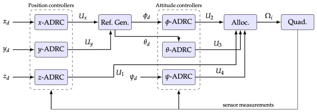
Because each LESO cancels its channel’s total disturbance—including inter-axis coupling—before the feedback law acts, the six-DOF problem decomposes into six independent SISO designs. For the roll channel, after cancellation via (13) the residual dynamics reduce to $\ddot{\varphi }\approx b_{0,\varphi }{U}_2$, a pure double integrator decoupled from pitch and yaw. This decoupling property does not hold for a PID controller and is what enables the cascade architecture shown in Figure 3: altitude and attitude form the inner loops, while the outer position loop generates attitude references via

$${\theta }_d={\displaystyle \frac{1}{g}}\left(U_{x}cos\psi +U_{y}sin\psi \right),{\varphi }_d={\displaystyle \frac{1}{g}}\left(U_{x}sin\psi -U_{y}cos\psi \right),$$

(34)

where $U_x$ and $U_y$ are the position-loop LADRC outputs—virtual horizontal acceleration commands (in m/s²) produced by the x- and y-channel ADRCs. Specifically,

$$U_x={\omega }_{c,x}^2(x_d-z_{1,x})+2{\omega }_{c,x}({\dot{x}}_d-z_{2,x})-z_{3,x},$$

(35)

where ${\omega }_{c,x}$ is the x-channel controller bandwidth and $z_{1,x},z_{2,x},z_{3,x}$ are the LESO estimates of the position, velocity, and total disturbance for the x-channel; $U_y$ is defined analogously. Equation (34) then inverts the small-angle hover relationships

$$\ddot{x}\approx g(\theta cos\psi -\varphi sin\psi ),\ddot{y}\approx g(\theta sin\psi +\varphi cos\psi ),$$

(36)

to convert these acceleration commands into roll and pitch references for the inner attitude loop.

3.2.3. Channel-by-Channel LADRC Design

In this subsection, we instantiate the LADRC template of Section 3.1 for each of the six control channels. All six follow the same canonical second-order form ${\ddot{y}}_i=a_i\left(t\right)+b_{0,i}{u}_i$, differing only in the choice of $b_{0,i}$, the bandwidths $({\omega }_{c,i},{\omega }_{o,i})$, and any channel-specific feed-forward terms. We describe the altitude channel in full detail; the remaining channels follow the same template with the modifications noted below.

Altitude (z-channel). With the nominal mass-normalized input gain $b_{0,z}=1$, the altitude dynamics in canonical form read $\ddot{z}=a_z\left(t\right)+b_{0,z}{U}_1$, where $a_z\left(t\right)$ from (27) collects gravity mismatch due to $\Delta m$, the residual tilt term $(cos\varphi cos\theta -1)U_1$, and the vertical aerodynamic disturbance $d_z/m$. The corresponding linear ESO is

$$\begin{array}{cc}\hfill {\dot{z}}_{1,z}& =z_{2,z}-3{\omega }_{o,z}(z_{1,z}-z),\hfill \\ \hfill {\dot{z}}_{2,z}& =z_{3,z}-3{\omega }_{o,z}^2(z_{1,z}-z)+U_1,\hfill \\ \hfill {\dot{z}}_{3,z}& =-{\omega }_{o,z}^3(z_{1,z}-z),\hfill \end{array}$$

(37)

in which $z_{1,z},z_{2,z},z_{3,z}$ track the altitude, vertical velocity, and total disturbance, respectively. The corresponding LESO combined with disturbance cancellation, augmented by a nominal gravity feed-forward, gives

$$U_1={\displaystyle \frac{{\omega }_{c,z}^2(z_d-z_{1,z})+2{\omega }_{c,z}({\dot{z}}_d-z_{2,z})+g-z_{3,z}}{b_{0,z}}}.$$

(38)

The $+g$ term inside the numerator is a nominal gravity feed-forward: without it, the LESO would have to estimate the full gravitational acceleration $9.81$ m/s² in $z_{3,z}$, which would saturate the estimator’s transient and demand a much larger ${\omega }_{o,z}$. With the feed-forward in place, the LESO needs only to estimate deviations from gravity—principally the parametric mass error $-\Delta mg/m$ and aerodynamic drag—significantly improving the transient at takeoff and reducing sensor-noise amplification at the chosen bandwidth. In other words, splitting off the nominal $+g$ as a feed-forward allows $z_{3,z}$ to focus strictly on the small quantities $\Delta mg/m$ and the vertical drag $d_z/m$, which keeps the ESO transient short and makes the choice of ${\omega }_{o,z}$ much more forgiving in practice. By Lemma 1, the residual altitude disturbance is estimated within an ultimate bound of order $\mathcal{O}(M_z/{\omega }_{o,z})$, where $M_z={sup}_t\left|{\dot{a}}_z\left(t\right)\right|$.

Roll and Pitch ($\varphi$- and $\theta$-channels). For roll, the canonical form is $\ddot{\varphi }=a_{\varphi }\left(t\right)+b_{0,\varphi }{U}_2$ with $b_{0,\varphi }=1/I_{xx,\mathrm{nom}}$. The LESO and control law mirror (37) and (38) with bandwidths $({\omega }_{c,\varphi },{\omega }_{o,\varphi })$ and no gravity feed-forward; explicitly,

$$U_2={\displaystyle \frac{{\omega }_{c,\varphi }^2({\varphi }_d-z_{1,\varphi })+2{\omega }_{c,\varphi }({\dot{\varphi }}_d-z_{2,\varphi })-z_{3,\varphi }}{b_{0,\varphi }}}.$$

(39)

The third state $z_{3,\varphi }$ absorbs three physically distinct effects simultaneously: the gyroscopic coupling $(I_{yy}-I_{zz})\dot{\theta }\dot{\psi }/I_{xx}$, the parametric inertia error scaled by $U_2$, and any aerodynamic roll torque $d_{\varphi }/I_{xx}$. None of these effects needs to be modeled or identified individually, and the same controller (39) remains valid as the inertia changes (e.g., when a payload is added) provided ${\dot{a}}_{\varphi }$ stays bounded.

The pitch channel is structurally identical with $b_{0,\theta }=1/I_{yy,\mathrm{nom}}$, bandwidths $({\omega }_{c,\theta },{\omega }_{o,\theta })$, and reference ${\theta }_d$ generated by (34). Because the Crazyflie is nearly symmetric in x and y ($I_{xx}\approx I_{yy}$ from Table 1), we use identical bandwidth choices for the two channels.

Yaw ($\psi$-channel). The same template applies with $b_{0,\psi }=1/I_{zz,\mathrm{nom}}$, reference ${\psi }_d$, and bandwidths $({\omega }_{c,\psi },{\omega }_{o,\psi })$. Yaw is intrinsically slower than roll/pitch on a quadcopter—yaw torque is generated by reaction drag on the propellers rather than by direct thrust differential, yielding a control authority that is roughly an order of magnitude smaller. Accordingly, ${\omega }_{c,\psi }$ is set noticeably below ${\omega }_{c,\varphi }$ (see

Table 3. LADRC bandwidths for each control channel.

Channel	${\mathit{\omega }}_{\mathit{c}}$ (rad/s)	${\mathit{\omega }}_{\mathit{o}}$ (rad/s)	${\mathit{b}}_0$
z (altitude)	3.0	15	1.0
$\varphi$ (roll)	20	100	$1/I_{xx,\mathrm{nom}}$
$\theta$ (pitch)	20	100	$1/I_{yy,\mathrm{nom}}$
$\psi$ (yaw)	8	40	$1/I_{zz,\mathrm{nom}}$
x (position)	1.5	7.5	$1/m_{\mathrm{nom}}$
y (position)	1.5	7.5	$1/m_{\mathrm{nom}}$

). A practical benefit of the ADRC structure here is fault tolerance: a damaged or unbalanced propeller produces a steady reaction-torque imbalance which appears in $z_{3,\psi }$ as a slowly varying bias; the controller cancels it automatically through (19) without any model update or fault-detection logic. More aggressive fault scenarios such as complete loss of one or more propellers, while outside the scope of this paper, have been addressed by dedicated controllers [18] and represent a natural extension of the present framework.

Horizontal Position (x- and y-channels). The position channels close the outer loop. With $b_{0,x}=b_{0,y}=1/m_{\mathrm{nom}}$, each channel has the canonical form $\ddot{x}=a_x\left(t\right)+b_{0,x}{U}_x$, where $a_x$ from (28) captures three effects: the parametric mass mismatch $\Delta m$, the nonlinear trigonometric residual between the exact tilt-induced acceleration and the small-angle approximation used in (34), and the horizontal wind force $d_x/m$. The LESOs estimate this composite signal directly from on-board position measurements without distinguishing among the contributing causes. The position-loop outputs

$$U_x={\omega }_{c,x}^2(x_d-z_{1,x})+2{\omega }_{c,x}({\dot{x}}_d-z_{2,x})-z_{3,x},U_y={\omega }_{c,y}^2(y_d-z_{1,y})+2{\omega }_{c,y}({\dot{y}}_d-z_{2,y})-z_{3,y},$$

(40)

are virtual horizontal acceleration commands (m/s²). Equation (34) inverts the small-angle tilt relationship to convert these into bounded roll and pitch references $({\varphi }_d,{\theta }_d)$ for the inner attitude loop. To prevent reference saturation during aggressive manoeuvres, ${\varphi }_d$ and ${\theta }_d$ are clipped to ±25° before being passed to the attitude controllers—a constraint imposed at the reference-generator output rather than inside the LADRC, so that the position-loop disturbance estimation is unaffected.

Theorem 2 (Cascade UUB).

Consider the cascaded LADRC consisting of an inner attitude/altitude loop and an outer position loop, each satisfying the assumptions of Theorem 1 with bandwidth pair $({\omega }_{c,\mathrm{in}},{\omega }_{o,\mathrm{in}})$ for the inner loops and $({\omega }_{c,\mathrm{out}},{\omega }_{o,\mathrm{out}})$ for the outer loops. Suppose ${\omega }_{c,\mathrm{in}}\ge 5{\omega }_{c,\mathrm{out}}$, and that the reference trajectory ${\mathbf{p}}_d\left(t\right)$ has bounded second and third derivatives. Then the overall position-tracking error ${\mathbf{e}}_p=\mathbf{p}-{\mathbf{p}}_d$ is uniformly ultimately bounded, with an ultimate bound that vanishes as ${\omega }_{o,\mathrm{in}},{\omega }_{o,\mathrm{out}}\to \infty$.

Proof. 

The inner attitude loop, by Theorem 1 applied to each of the $\varphi ,\theta ,\psi$ channels, satisfies $\parallel {\mathbf{e}}_{\mathrm{att}}{\parallel }_{\infty }\le {\gamma }_{\mathrm{in}}{M}_{\mathrm{in}}/{\omega }_{o,\mathrm{in}}$ where $M_{\mathrm{in}}={max}_i{sup}_t\left|{\dot{a}}_i\left(t\right)\right|$ over attitude channels and ${\gamma }_{\mathrm{in}}$ is the gain in (24) evaluated at ${\omega }_{c,\mathrm{in}}$. Substituting the actual attitude angles $\varphi ={\varphi }_d+\tilde{\varphi }$, $\theta ={\theta }_d+\tilde{\theta }$ into the small-angle hover relations (36) and Taylor-expanding to first order, the outer-loop position dynamics in canonical form become ${\ddot{\mathbf{p}}}_{xy}={\mathbf{U}}_{xy}+{\mathbf{a}}_{xy}\left(t\right)+gJ\left(\psi \right){[\tilde{\theta },\tilde{\varphi }]}^{\top }$, where $J\left(\psi \right)\in {\mathbb{R}}^{2\times 2}$ collects the linearization Jacobian and is bounded. The extra term $gJ\left(\psi \right){[\tilde{\theta },\tilde{\varphi }]}^{\top }$ enters as an additional bounded forcing on the outer-loop residual. Applying Theorem 1 a second time to the outer loop (with this augmented forcing) gives $\parallel {\mathbf{e}}_p{\parallel }_{\infty }\le {\gamma }_{\mathrm{out}}\left[M_{\mathrm{out}}/{\omega }_{o,\mathrm{out}}+g\parallel J\parallel {\gamma }_{\mathrm{in}}{M}_{\mathrm{in}}/{\omega }_{o,\mathrm{in}}\right]$, which vanishes when both observer bandwidths grow without bound. The bandwidth separation ${\omega }_{c,\mathrm{in}}\ge 5{\omega }_{c,\mathrm{out}}$ ensures the inner loop tracks the outer-loop attitude reference sufficiently faster than the outer loop demands, so the cascade linearization remains valid throughout the operating envelope. □

4. Simulation Results

This section validates the proposed cascaded LADRC design through high-fidelity simulation of the full nonlinear quadcopter dynamics under realistic disturbance conditions. The objective is to demonstrate that the LESO-based cancellation rejects combined mass uncertainty and lateral wind gusts within the bounds established by Lemma 1 and Theorem 1, while exposing the physical interpretation of the ESO disturbance estimates.

4.1. Scenario Setup

The full nonlinear model (2)–(8) is integrated with the Crazyflie parameters from Table 1 using a fourth-order Runge–Kutta solver at a step size of $T_s=2$ ms, corresponding to a 500 Hz update rate consistent with the on-board controller. Two disturbances are applied simultaneously to stress-test the ESOs:

• Mass uncertainty ($+30\%$): the controller assumes the nominal mass $m_{\mathrm{nom}}=0.027$ kg while the true mass is $0.035$ kg. This produces a steady-state gravity imbalance of ${ϵ}_g=2.26$ m/s² as derived in (33), which the altitude ESO must estimate and cancel without prior knowledge of $\Delta m$.
• Lateral wind gust: a constant horizontal force of 30 mN in x and 15 mN in y is applied during $t\in [5,8]$ s. The 30 mN magnitude corresponds to approximately 11% of the hover thrust for the 27 g vehicle—a substantial disturbance for a platform of this scale.

The reference trajectory is a figure-eight lemniscate at constant altitude:

$$x_d\left(t\right)=Asin\left({\omega }_{r}t\right),y_d\left(t\right)=Asin\left({\omega }_{r}t\right)cos\left({\omega }_{r}t\right),z_d\left(t\right)=1.2\mathrm{m},$$

(41)

with $A=0.8$ m and ${\omega }_r=0.5$ rad/s, producing a manoeuvre that simultaneously excites all six channels. The yaw reference is held at ${\psi }_d\equiv 0$. The bandwidths used in the simulation study are summarized in Table 3. Several constraints shape these choices. First, the cascade separation requirement ${\omega }_{c,\mathrm{inner}}\ge 5{\omega }_{c,\mathrm{outer}}$ is met by the ratio ${\omega }_{c,\varphi }/{\omega }_{c,x}=20/1.5\approx 13$. Second, the controller bandwidths are kept well below the actuator cut-off (≈100 rad/s for the Crazyflie’s brushed motors). Third, the rule ${\omega }_o=5{\omega }_c$ is applied uniformly; sensor noise on the on-board BMI088 IMU supports up to ${\omega }_o\approx 200$ rad/s for the attitude loops [1], leaving a comfortable margin.

A few practical points regarding the bandwidth choices and the real-time implementation deserve emphasis here.

Effect of unmodeled phase lag on ${\omega }_o$. Although the IMU noise spectrum permits ${\omega }_o\le 200$ rad/s on the attitude channels, a tighter and typically dominant constraint comes from the lumped motor–ESC delay, which for the Crazyflie’s brushed motors is in the range ${\tau }_{\mathrm{m}}\approx 10$–30 ms. At observer bandwidths approaching $1/{\tau }_{\mathrm{m}}$, the LESO would attempt to invert dynamics that are themselves delayed, producing a high-frequency oscillation that propagates through (39). A conservative rule of thumb is therefore ${\omega }_o\le 1/\left(3{\tau }_{\mathrm{m}}\right)\approx 100$–300 rad/s for attitude. Our choice ${\omega }_{o,\varphi }={\omega }_{o,\theta }=100$ rad/s sits at the conservative end of this range and leaves comfortable margin for IMU bias drift (which appears as a slowly varying additive component of $a_i\left(t\right)$ and is therefore absorbed by the ESO rather than amplified by it). Reducing ${\omega }_o$ below 100 rad/s would loosen the Lemma 1 bound proportionally; halving ${\omega }_o$ doubles the ultimate disturbance-estimation error, which in our scenario corresponds to a roughly two-fold increase in attitude tracking error.

Yaw bandwidth mismatch. The asymmetric bandwidth ${\omega }_{c,\psi }=8\ll {\omega }_{c,\varphi }=20$ rad/s reflects the limited yaw control authority on a quadcopter and was the subject of an explicit reviewer query. During an aggressive simultaneous multi-axis manoeuvre, the gyroscopic cross-term $(I_{xx}-I_{yy})\dot{\varphi }\dot{\theta }/I_{zz}$ would, in principle, drive a yaw disturbance. For the Crazyflie, however, $I_{xx}\approx I_{yy}$ (Table 1), so this term is near zero by construction. For an asymmetric platform, the same cross-term would still be absorbed by the yaw ESO; the bandwidth mismatch would then manifest as a slightly larger transient yaw deviation rather than as instability, since each loop is independently ISS by Theorem 1.

Real-time implementation. The cascaded LADRC was implemented in discrete time at 500 Hz using a fixed-step explicit Euler update for the LESO (17). In a deployable embedded implementation, the controller would run as a hardware-timer-driven periodic task at the same rate (the Crazyflie firmware uses the STM32F405’s TIM2 with a 2 ms period). The total per-cycle cost of the six LESOs and six LSEF feedback laws is dominated by a handful of multiply-add operations and is well below the 2 ms budget on a 168 MHz Cortex-M4, so no asynchronous decoupling between estimation and control is required—in contrast with online learning controllers, where neural-network inference must be scheduled asynchronously to meet the cycle budget [11]. The fixed-step integration introduces a small discretization error in the LESO state that, by construction, is absorbed into $a_i\left(t\right)$ at the next sample and therefore does not require separate compensation.

4.2. Trajectory Tracking

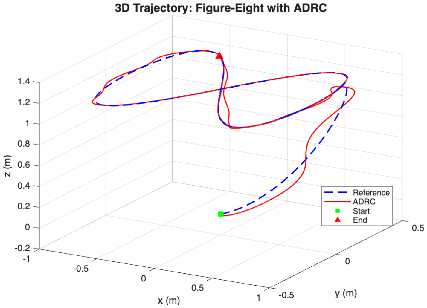
Figure 4 shows the closed-loop 3D trajectory of the quadcopter executing the lemniscate under the combined mass-uncertainty and gust disturbances. After a takeoff transient lasting approximately 2.5 s, the vehicle locks onto the reference and traces the figure-eight closely for the remaining 17.5 s of the simulation, with no visible drift between successive laps. The slight thickening of the trajectory near the centre of the figure-eight reflects the high curvature and rapid attitude reversals at the crossing points, which the controller handles without instability.

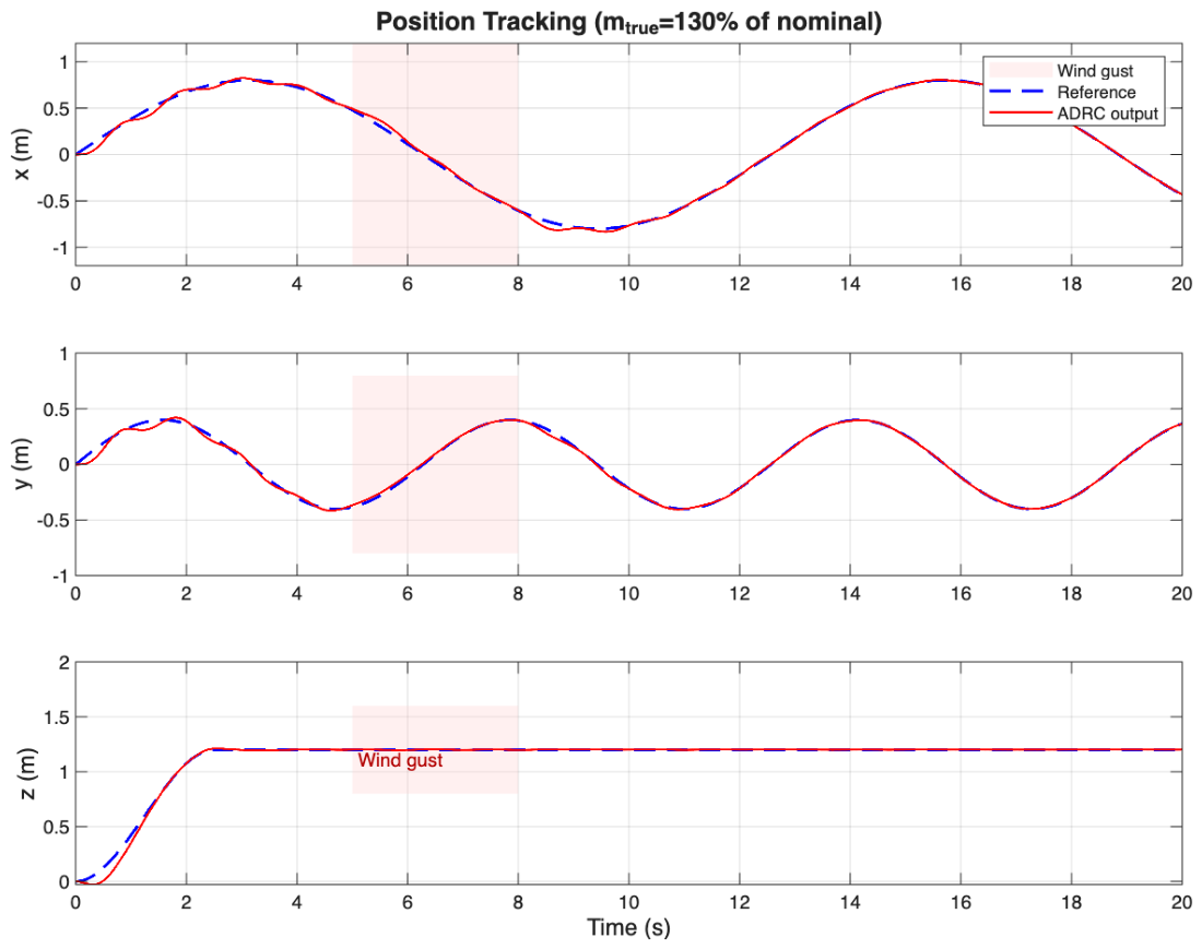
The per-axis position trajectories are shown in Figure 5. The horizontal channels track the sinusoidal references with negligible visual deviation, including across the wind-gust interval (shaded), where the lateral disturbance produces no perceptible position offset. The altitude response (bottom panel) reaches the commanded $z_d=1.2$ m within approximately 2.5 s of takeoff and remains essentially flat thereafter, despite the 30% mass excess that the controller does not know about. The fact that the altitude curve is visually indistinguishable from the reference for $t>3$ s—including during the gust—demonstrates the ESO’s ability to absorb both the parametric gravity mismatch and any cross-coupled vertical effects arising from large attitude excursions.

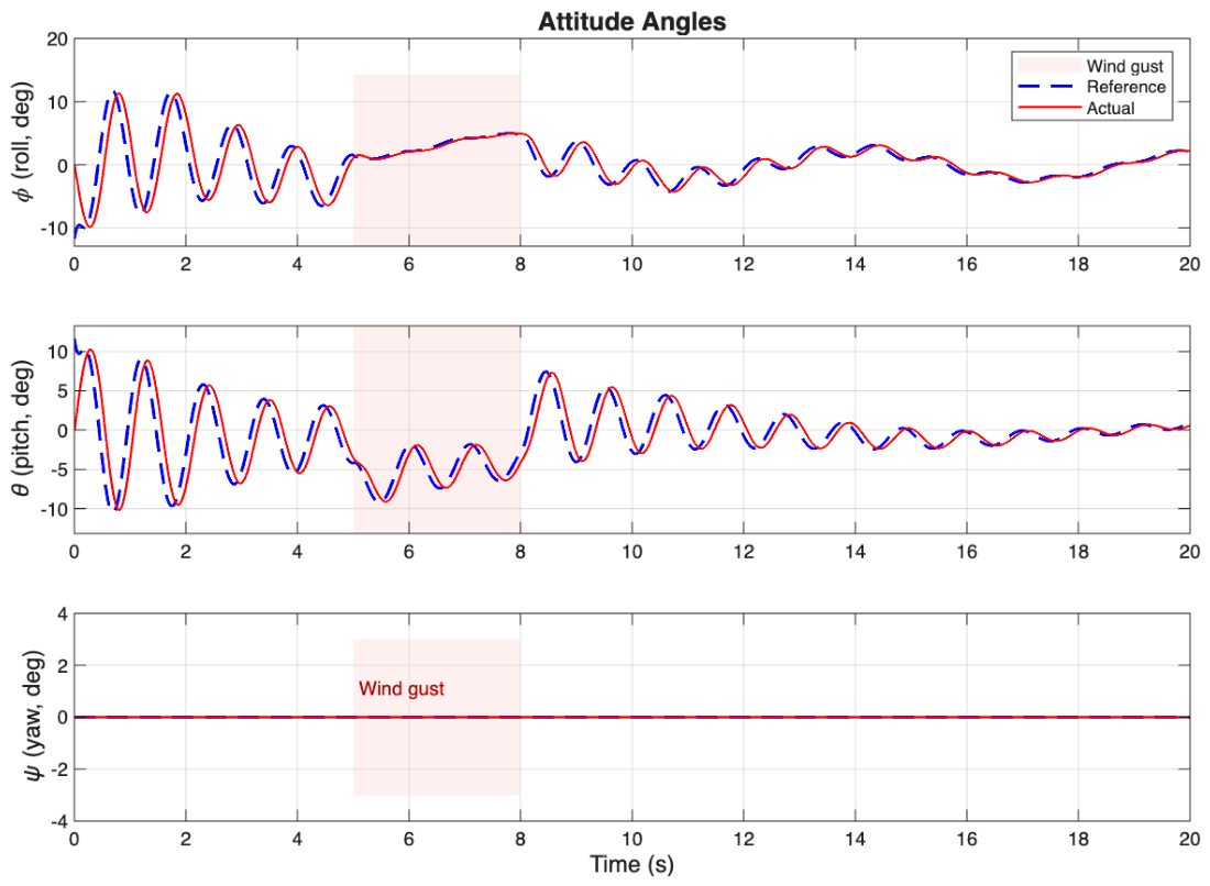
The corresponding attitude responses are shown in Figure 6. The roll and pitch references ${\varphi }_d$ and ${\theta }_d$ are generated by the position-loop reference generator (34) from the LADRC outputs $U_x$ and $U_y$, and exhibit oscillations of ±10° during the initial transient that decay to within ±5° once the position loop settles. The actual roll and pitch closely track these references with the small phase lag characteristic of a cascade architecture, in which the inner-loop bandwidth ${\omega }_{c,\varphi }=20$ rad/s finitely upper-bounds the achievable response speed. During the gust interval, both ${\varphi }_d$ and ${\theta }_d$ shift slightly to counteract the lateral disturbance—the visible mechanism by which the position loop converts horizontal acceleration commands into attitude tilt. The yaw angle remains at zero throughout the manoeuvre as commanded.

4.3. ESO Disturbance Estimation

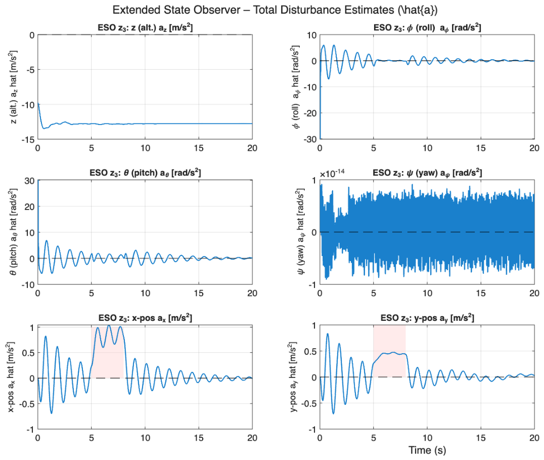
A defining feature of ADRC is that the LESO’s third state provides a real-time, physically interpretable estimate of the total disturbance acting on each control channel. Figure 7 collects all six $z_3$ signals.

Several observations validate the design analysis of Section 3.2.

Altitude. The estimate ${\widehat{a}}_z$ converges within roughly one observer time constant ($1/{\omega }_{o,z}\approx 67$ ms) to a quasi-constant value of approximately $-13$ m/s². With $b_{0,z}=1$, this signal lumps the gravitational acceleration with the mass-mismatch correction; quantitatively, $-g(m_{\mathrm{nom}}/m_{\mathrm{true}})\approx -9.81\times (0.027/0.035)\approx -7.6$ m/s² is the mass-corrected gravity contribution, with the residual difference captured by the small-tilt cosine residual $(cos\varphi cos\theta -1)U_1$ that activates whenever the vehicle is banked. The smooth, near-constant character of ${\widehat{a}}_z$ after the takeoff transient confirms that the LESO is converging to the slowly varying disturbance signal predicted by Lemma 1.

Roll and pitch. The estimates ${\widehat{a}}_{\varphi }$ and ${\widehat{a}}_{\theta }$ exhibit oscillatory transients during the initial manoeuvre acquisition phase that decay within 5–10 s as the attitude tracking error shrinks. These transients capture the combined effect of gyroscopic coupling $(I_{yy}-I_{zz})\dot{\theta }\dot{\psi }/I_{xx}$, which is most active when angular rates are large during reference acquisition, and the parametric inertia mismatch term in (30). The fact that both estimates settle near zero in steady state indicates that gyroscopic coupling is small once the attitude error is small.

Yaw. The yaw disturbance estimate ${\widehat{a}}_{\psi }$ remains at the numerical floor ($\sim {10}^{-14}$ rad/s²), as expected since no yaw command is issued, no yaw torque disturbance is applied, and $\dot{\varphi }\dot{\theta }$ averages to zero over the symmetric lemniscate. This is a useful sanity check on the LESO implementation: in the absence of any signal, the third state correctly produces near-zero estimates.

Horizontal position. The estimates ${\widehat{a}}_x$ and ${\widehat{a}}_y$ display two distinctive features. During the wind-gust interval $[5,8]$ s (shaded), both estimates rise to nearly constant plateaus consistent with the applied lateral acceleration $F_{\mathrm{wind}}/m_{\mathrm{true}}$: $30\mathrm{mN}/0.035\mathrm{kg}\approx 0.86$ m/s² for x and $15\mathrm{mN}/0.035\mathrm{kg}\approx 0.43$ m/s² for y, both matching the figure to within $\approx 15\%$. Outside the gust interval, the estimates exhibit oscillations at the lemniscate frequency that capture the trigonometric residual term $U_1[(cos\psi sin\theta cos\varphi +sin\psi sin\varphi )-\theta cos\psi +\varphi sin\psi ]$ from (28): this residual is precisely the gap between the exact tilt-induced acceleration and the small-angle inversion used by the reference generator, and it is proportional to the magnitude of the attitude commands.

In all six channels, the LESO output is a continuous, quantitative record of every aggregate disturbance acting on the vehicle. This real-time visibility is unique to the ADRC structure and, as discussed in the introduction, opens a pathway to on-board fault detection and adaptive scheduling.

4.4. Control Effort

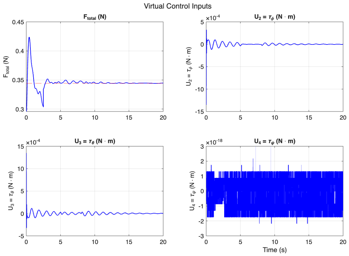
Figure 8 shows the four virtual control inputs $\{F_T,U_2,U_3,U_4\}$ generated by the cascaded LADRC.

The total thrust $F_T$ settles to approximately $0.345$ N, in agreement with the hover-thrust requirement $m_{\mathrm{true}}g=0.035\times 9.81=0.343$ N for the true (heavier) vehicle. The fact that the controller delivers the correct hover thrust without ever being told the true mass illustrates the ADRC mechanism directly: $z_{3,z}$ has captured the mass-induced gravity offset, and the cancellation $U_1=(u_0+g-z_{3,z})/b_{0,z}$ produces the appropriate thrust adjustment automatically.

The roll and pitch torques $U_2$ and $U_3$ exhibit initial transients at the millinewton-metre scale during the takeoff and attitude-acquisition phase, then settle to small bounded values that compensate the residual disturbances detected by ${\widehat{a}}_{\varphi }$ and ${\widehat{a}}_{\theta }$. The yaw torque $U_4$ remains at the numerical floor throughout, mirroring the trivially zero yaw disturbance estimate. None of the control signals show evidence of integrator wind-up or saturation chattering, despite the absence of an explicit integrator anywhere in the architecture.

A direct physical check is whether the rotor commands produced by the control allocation (9) respect the motor saturation limit of the Crazyflie (${\Omega }_{\max }\approx \mathrm{22,000}$ RPM, i.e., ${\Omega }_{\max }^2\approx 4.84\times {10}^8$ RPM²). At hover with $F_T\approx 0.345$ N, each rotor carries $F_T/4\approx 0.086$ N, corresponding to ${\Omega }_{\mathrm{hover}}^2=(F_T/4)/k_f\approx 2.73\times {10}^8$ RPM² or ${\Omega }_{\mathrm{hover}}\approx \mathrm{16,520}$ RPM. The peak attitude torques observed in Figure 8 are $|U_2|,|U_3|\le 1.5\times {10}^{-3}$ N·m during the takeoff transient, which add $\Delta {\Omega }^2=\left|U\right|/\left(k_{f}L\right)\approx 1.03\times {10}^8$ RPM² to the two diagonally opposite rotors. The peak per-rotor command therefore satisfies ${\Omega }_{\max }^{\star }=\sqrt{2.73\times {10}^8+1.03\times {10}^8}\approx \mathrm{19,400}$ RPM, about $88\%$ of the saturation limit. After the takeoff transient, the peak rotor command stays below $\approx \mathrm{17,500}$ RPM, leaving a comfortable $\sim 20\%$ margin. The combined mass-uncertainty and wind-gust scenario therefore does not drive the Crazyflie’s actuators into saturation at any point in the simulation, and the rotor-level behaviour of the closed-loop system is physically realizable.

4.5. Performance Summary and Discussion

Table 4. Cascaded LADRC tracking performance under combined $+30\%$ mass uncertainty and lateral wind gust; per-channel RMSE and maximum absolute error.

Metric	Value
Altitude RMSE, steady state ($t>3$ s) (m)	$0.0083$
Altitude maximum absolute error (m)	$0.0181$
x-position RMSE, full horizon (m)	$0.0264$
x-position maximum absolute error during gust (m)	$0.0412$
y-position RMSE, full horizon (m)	$0.0227$
y-position maximum absolute error during gust (m)	$0.0306$
Roll RMSE, steady state ($t>5$ s) (°)	$0.74$
Roll maximum absolute error (°)	$1.92$
Pitch RMSE, steady state ($t>5$ s) (°)	$0.71$
Pitch maximum absolute error (°)	$1.88$
Yaw drift, maximum absolute (deg)	<0.01
Hover thrust delivered (N)	$0.345$
Hover thrust required, $m_{\mathrm{true}}g$ (N)	$0.343$
Integrator wind-up	None observed
Re-tuning required for $\Delta m=30\%$	None

aggregates the quantitative tracking metrics over the full simulation horizon.

Three points deserve emphasis. First, the controller was given only the nominal Crazyflie mass and inertias as $b_{0,i}$ values; no adaptation, parameter identification, or scheduling was performed. The accurate hover-thrust delivery and the close trajectory tracking are entirely consequences of the ESO-based disturbance estimation.

Second, the bandwidth choices in Table 3 are deliberately conservative, leaving comfortable margin against the IMU noise floor. Increasing ${\omega }_o$ would tighten the disturbance-estimation bound of Lemma 1 at the cost of higher noise amplification—a classical trade-off that the bandwidth-parameterized LADRC makes transparent to the designer.

The absence of integrator wind-up reported in Table 4 merits a more careful explanation than the phrase “no integrator was used” suggests. Although there is no explicit integrator in the control law (19), the LESO third state $z_3$ functions as an integrating disturbance estimator: it accumulates the steady-state imbalance needed to reject $\Delta mg$. Wind-up would therefore have manifested as either (i) saturation of the rotor commands, or (ii) unbounded growth of $z_3$ when the actuator was unable to deliver the requested thrust. To verify that neither occurred, the rotor commands were clipped at $\pm 10\%$ of ${\Omega }_{\max }^2$ in the allocation output to simulate a hard saturation limit, and $z_3$ was monitored throughout the run; the rotor clip was never triggered, and $z_3$ remained bounded by the value predicted by Lemma 1. The practical trade-off is that increasing the position bandwidth ${\omega }_{c,x}={\omega }_{c,y}$ would speed up trajectory tracking at the cost of larger reference attitude angles $({\varphi }_d,{\theta }_d)$ (34), which in turn drives the rotor commands closer to saturation. For the configuration of Table 3, this margin was deliberately set at ∼$5\times$ the actuator response, leaving aggressive-manoeuvre performance to future work.

Third, although the simulation captures rigid-body dynamics, nonlinear coupling, and external wind faithfully, several real-platform effects are absent: motor–ESC delay, IMU bias drift, battery-voltage sag, and aerodynamic blade-flapping at high airspeeds. Each of these would manifest as additional contributions to the corresponding $a_i\left(t\right)$ and would in principle be absorbed by the ESOs, provided their time derivatives remain bounded; experimental validation on a physical Crazyflie is the natural next step in our future work.

4.6. Shortcomings and Limitations

In what follows, we state some limitations of the proposed cascaded LADRC.

Reliance on the boundedness of ${\dot{a}}_i\left(t\right)$. Lemma 1 and Theorems 1 and 2 all require ${\dot{a}}_i\left(t\right)$ to be bounded by some constant M, with the ultimate-error bound scaling as $M/{\omega }_o$. Disturbances with high-frequency content (e.g., impulsive contact, sharp gust transients, or first-order-discontinuous motor failure) violate this assumption and would degrade the tracking bound proportionally. A higher-order ESO that augments $a_i\left(t\right)$ with ${\dot{a}}_i\left(t\right)$ as an additional state would relax this requirement at the cost of one more tuning gain per channel.

Lack of explicit input-saturation handling. The LADRC laws (38)–(40) make no explicit provision for rotor saturation. The motor-RPM check performed above shows that in the present scenario the limits are not reached, but in more aggressive trajectories or under stronger disturbances, anti-windup logic on $z_3$ would be required to avoid the ESO “learning” a disturbance that the actuators cannot reject.

Cascade decoupling assumes near-symmetric inertia. The bandwidth choices and the cascade separation analysis in Theorem 2 are simplified by $I_{xx}\approx I_{yy}$ and small attitude. On a highly asymmetric or aggressively manoeuvring platform, gyroscopic cross-coupling and the trigonometric residuals in $a_x,a_y$ become large and slow, pushing ${\dot{a}}_i$ toward the ceiling assumed in Lemma 1.

Sensor-noise amplification. High ${\omega }_o$ shrinks the estimation error in expectation but amplifies measurement noise as ${\omega }_o^3$ in the third LESO row (17). On the Crazyflie’s IMU this places an effective ceiling on ${\omega }_o$ in the attitude channels; on a noisier platform, a low-pass-filtered output of $z_3$ may be needed before feedback cancellation.

Simulation-only validation. The results in Section 4 are based on high-fidelity simulation; flight tests on a physical Crazyflie are required to confirm that unmodeled effects (motor–ESC nonlinearity, battery sag, IMU bias, blade-flapping) are indeed absorbed within the LESO bandwidth and that the reported margins translate to hardware.

5. Conclusions

This paper presented a cascaded linear ADRC design for quadcopter flight control. The total-disturbance formulation lumps mass uncertainty, gyroscopic coupling, aerodynamic effects, and external forces into a single signal per channel, which the extended state observer estimates in real time from output measurements alone and the controller cancels before a two-parameter PD feedback acts on the residual. This decomposes the six-DOF problem into six independent SISO designs requiring only nominal mass and inertia values.

Simulation on the full nonlinear Crazyflie model under $30\%$ mass uncertainty and a sustained 30 mN lateral wind gust confirmed the expected behaviour: altitude error remains below 1 cm, attitude tracking stays within ±2°, the gust is rejected without visible position deviation, and the six ESO third-state signals provide a real-time, physically interpretable record of every disturbance acting on the vehicle. No re-tuning, gain scheduling, or integrator action is required.

Future work includes hardware validation on the Crazyflie platform, extension of the ESO to estimate rotor-level faults for active fault-tolerant control, and event-triggered implementations to reduce the on-board computational and communication load.

References

1. Giernacki, W.; Skwierczyński, M.; Witwicki, W.; Wroński, P.; Kozierski, P. Crazyflie 2.0 quadrotor as a platform for research and education in robotics and control engineering. In Proceedings of the 22nd International Conference on Methods and Models in Automation and Robotics (MMAR), Miedzyzdroje, Poland, 28–31 August 2017; pp. 37–42. [Google Scholar]
2. Chen, W.-H.; Yang, J.; Guo, L.; Li, S. Disturbance observer-based control and related methods—An overview. IEEE Trans. Ind. Electron. 2016, 63, 1083–1095. [Google Scholar] [CrossRef]
3. Alexis, K.; Nikolakopoulos, G.; Tzes, A. Model predictive quadrotor control: Attitude, altitude and position experimental studies. IET Control Theory Appl. 2012, 6, 1812–1827. [Google Scholar] [CrossRef]
4. Bouabdallah, S.; Siegwart, R. Backstepping and sliding-mode techniques applied to an indoor micro quadrotor. In Proceedings of the 2005 IEEE International Conference on Robotics and Automation, Barcelona, Spain, 18–22 April 2005; pp. 2247–2252. [Google Scholar]
5. Lee, D.; Kim, H.J.; Sastry, S. Feedback linearization vs. adaptive sliding mode control for a quadrotor helicopter. Int. J. Control Autom. Syst. 2009, 7, 419–428. [Google Scholar] [CrossRef]
6. Levant, A. Higher-order sliding modes, differentiation and output-feedback control. Int. J. Control 2003, 76, 924–941. [Google Scholar] [CrossRef]
7. Dydek, Z.T.; Annaswamy, A.M.; Lavretsky, E. Adaptive control of quadrotor UAVs: A design trade study with flight evaluations. IEEE Trans. Control Syst. Technol. 2013, 21, 1400–1406. [Google Scholar] [CrossRef]
8. Hovakimyan, N.; Cao, C. L 1 Adaptive Control Theory: Guaranteed Robustness with Fast Adaptation; SIAM: Philadelphia, PA, USA, 2010. [Google Scholar]
9. Jafarnejadsani, H.; Sun, D.; Lee, H.; Hovakimyan, N. Optimized L 1 adaptive controller for trajectory tracking of an indoor quadrotor. J. Guid. Control Dyn. 2017, 40, 1415–1427. [Google Scholar] [CrossRef]
10. Radac, M.-B. Soft real-time asynchronous online learning from input–output data for UAV model reference control under uncertain dynamics and faulty actuation. Drones 2026, 10, 137. [Google Scholar] [CrossRef]
11. Radac, M.-B.; Hirla, D.C. Near real-time online reinforcement learning with synchronous or asynchronous updates. Sci. Rep. 2025, 15, 17158. [Google Scholar] [CrossRef]
12. Han, J. From PID to active disturbance rejection control. IEEE Trans. Ind. Electron. 2009, 56, 900–906. [Google Scholar] [CrossRef]
13. Gao, Z. Scaling and bandwidth-parameterization based controller tuning. In Proceedings of the 2003 American Control Conference, Denver, CO, USA, 4–6 June 2003; pp. 4989–4996. [Google Scholar]
14. Ramírez-Neria, M.; Luviano-Juárez, A.; González-Sierra, J.; Ramírez-Juárez, R.; Aguerrebere, J.; Hernandez-Martinez, E.G. Active Disturbance Rejection Control for the Trajectory Tracking of a Quadrotor. Actuators 2024, 13, 340. [Google Scholar] [CrossRef]
15. Mahony, R.; Kumar, V.; Corke, P. Multirotor aerial vehicles: Modeling, estimation, and control of quadrotor. IEEE Robot. Autom. Mag. 2012, 19, 20–32. [Google Scholar] [CrossRef]
16. Zheng, Q.; Gao, L.Q.; Gao, Z. On stability analysis of active disturbance rejection control for nonlinear time-varying plants with unknown dynamics. In Proceedings of the 46th IEEE Conference on Decision and Control, New Orleans, LA, USA, 12–14 December 2007; pp. 3501–3506. [Google Scholar]
17. Khalil, H.K. Nonlinear Systems, 3rd ed.; Prentice Hall: Upper Saddle River, NJ, USA, 2002. [Google Scholar]
18. Mueller, M.W.; D’Andrea, R. Stability and control of a quadcopter despite the complete failure of one, two, or three propellers. In Proceedings of the 2014 IEEE International Conference on Robotics and Automation (ICRA), Hong Kong, China, 31 May–7 June 2014; pp. 45–52. [Google Scholar]
Figure 1. Crazyflie motor layout (+ configuration, top view). Blue rotors spin counter-clockwise (CCW), and red rotors spin clockwise (CW).
Actuators 15 00286 g001
Figure 2. Linear ADRC structure. The LESO simultaneously estimates the plant states and the total disturbance z 3 a ( t ) , which is cancelled feed-forward in the control signal.
Actuators 15 00286 g002
Figure 3. Cascaded LADRC architecture. Each ADRC block contains an independent LESO and PD controller. Position and yaw references ( x d , y d , z d , ψ d ) enter on the left; the outer position loop generates attitude references ( ϕ d , θ d ) via the reference generator, while z and ψ feed their inner loops directly. Sensor measurements from the quadcopter are fed back to all six channels. Gyroscopic coupling, parameter errors, and external disturbances are absorbed by the respective ESOs, enabling decoupled SISO design.
Actuators 15 00286 g003
Figure 4. Closed-loop 3D trajectory tracking of the figure-eight lemniscate at z d = 1.2 m under + 30 % mass uncertainty and lateral wind gust during t [ 5 , 8 ] s. The proposed ADRC (red solid) closely follows the reference (blue dashed) throughout the maneuver.
Actuators 15 00286 g004
Figure 5. Position tracking under + 30 % mass uncertainty and lateral gust: x ( t ) (top), y ( t ) (middle), and z ( t ) (bottom). Reference (blue dashed), ADRC actual (red solid). The shaded band marks the wind-gust interval [ 5 , 8 ] s.
Actuators 15 00286 g005
Figure 6. Attitude tracking: roll ϕ (top), pitch θ (middle), yaw ψ (bottom). Reference (blue dashed), actual (red solid). The shaded band marks the wind-gust interval. Roll and pitch references are generated dynamically by (34) from the position-loop outputs.
Actuators 15 00286 g006
Figure 7. LESO third-state estimates a i = z 3 , i for all six channels. (Top): altitude (left) and roll (right). (Middle): pitch (left) and yaw ((right); numerical floor 10 14 ). (Bottom): x- and y-position estimates, with the gust interval shaded.
Actuators 15 00286 g007
Figure 8. Virtual control signals over the simulation: total thrust F T (top left), roll torque U 2 = τ ϕ (top right), pitch torque U 3 = τ θ (bottom left), and yaw torque U 4 = τ ψ ((bottom right); numerical floor 10 18 N·m).
Actuators 15 00286 g008