Article

Time-Varying Formation Tracking Control of Linear Multi-Agent Systems with Magnitude and Rate Saturation and Unknown Disturbances


1
College of Marine Electrical Engineering, Dalian Maritime University, Dalian 116026, China
2
College of Artificial Intelligence, Dalian Maritime University, Dalian 116026, China
*
Author to whom correspondence should be addressed.
Actuators 2026, 15(2), 110; https://doi.org/10.3390/act15020110
Submission received: 4 January 2026 / Revised: 30 January 2026 / Accepted: 3 February 2026 / Published: 9 February 2026
(This article belongs to the Section Control Systems)

Abstract

In this paper, we study the leader-following time-varying formation (TVF) tracking control of general linear multi-agent systems (MASs) with nonzero control input of the leader, and the followers which have magnitude and rate saturation (MRS) and unknown disturbances. Under the assumption that only the followers connecting to the leader have access to the leader’s input and state, an output feedback controller incorporating a distributed extended state observer (ESO) is developed to ensure the asymptotic convergence of the formation errors without input saturation. Then, a saturation model is inserted to each follower’s dynamics to constrain the magnitude and rate of the control input, with consideration of MRS. Anti-windup protection loops are applied to compensate for the saturated signals to improve the closed-loop performance. Finally, the theoretical findings are demonstrated via a series of numerical simulations.

1. Introduction

Over the past few decades, the cooperative control of multi-agent systems (MASs) has received widespread attention and is increasingly being applied in diverse fields including intelligent transportation, maritime patrol, aerospace, and smart factories [1,2,3,4,5]. Its objective is to guide all agents in achieving and maintaining a desired configuration according to task requirements. In Ref. [6], time-varying formation (TVF) tracking for second-order systems is addressed by using the relative information of the neighboring agents under switching topologies. In Ref. [7], a distributed controller is designed for high-order MASs to achieve the desired formation. In Ref. [8], the analysis and design of formation–containment control are investigated for high-order linear time-invariant MASs with time delays under directed interaction topologies. Reference [9] introduces a novel consensus control strategy for MASs comprised of electromechanical actuators. In Ref. [10], a general TVF tracking is proposed for general linear MASs with time delays. Under switching directed topology, the TVF of general linear MASs is solved in [11]. In Ref. [12], TVF with multiple leaders is discussed for general linear MASs. The TVF tracking problem is investigated for multi-leader MASs under sampled-data control in [13]. In Ref. [14], the output TVF tracking problem of heterogeneous MASs under model uncertainties and external disturbances is explored by an adaptive event-triggered mechanism. In Ref. [15], the TVF problem is studied for general linear MASs with unknown tracking leader inputs. The adaptive TVF containment tracking problem is discussed based on state observers for general linear MASs with unknown and bounded leaders’ inputs in [16]. For more recent works on TVF, please see refs. [17,18,19,20] and the references therein.
In practical implementations, MASs inevitably face external disturbances, which can weaken their ability to achieve predetermined configurations. One way to deal with the disturbances or uncertainties in solving formation control is to combine the consensus theory of MASs and the traditional robust control theory of single systems. Considerable efforts have extended robust control methods from single systems to MASs for consensus control. In Ref. [21], adaptive robust TVF tracking control for high-order linear MASs with uncertainties and external disturbances is investigated, where the leader is subject to a nonzero control input. In Ref. [22], the robust H 2 consensus problem of linear MASs is solved with parametric uncertainties and noise signals. In Ref. [23], a distributed L 2 robust control strategy is proposed for heterogeneous MASs subject to uncertainties and disturbances to achieve TVF under static and switching topologies. The robust TVF tracking for modified high-order linear MASs with heterogeneous uncertainties, external disturbances and unknown leader input is studied in Ref. [24]. The TVF H control problem of heterogeneous MASs subject to uncertainties and external disturbances under static and switching topologies is studied by the internal model-based robust formation controllers in [25]. In Ref. [26], the robust H output TVF problem for heterogeneous nonlinear MASs is investigated, where the actuator faults and external disturbances are considered. The TVF for general linear MASs with external disturbances and time delays is addressed in [27], where the influence of the disturbances is minimized by optimizing the H performance index. Another method is based on an extended state observer (ESO), where the disturbances or uncertainties are treated as additional states and compensated in the control design process. Compared with the robust control method, the ESO-based control shows excellent performance in estimating the disturbances or uncertainties. In Ref. [28], the leader-following tracking problem for general linear MASs under unknown disturbances is addressed using a distributed ESO. In Ref. [29], the formation control problem is studied for second-order nonlinear MASs with ESO. In Ref. [30], an ESO-based distributed model predictive control method is proposed for multi-robot formation under unknown disturbances. In Ref. [31], practical TVF tracking for high-order nonlinear MASs is studied using a distributed disturbance observer under directed topologies, ensuring arbitrarily small tracking errors. In Ref. [32], a robust TVF problem for second-order MASs subjected to external disturbances is investigated by ESO. In Ref. [33], the TVF is solved for second-order nonlinear MASs subject to uncertainties by event-triggered fuzzy ESO. Finite-time formation control for multi-UAVs with actuator faults and unmeasurable states is achieved using an ESO that estimates uncertainties, disturbances, and faults in [34]. A prescribed-time ESO is developed to compensate for external disturbances and internal unknown dynamics for vehicles to solve formation control strategy in [35]. Based on the aforementioned articles, few works have considered the TVF tracking control of high-order linear MASs with unknown disturbances and nonzero leader inputs by using ESO, which is one of the motivations of this study.
Actuator saturation arising from physical constraints and safety requirements may also degrade system performance or destabilize the system. In Ref. [36], a saturated formation tracking controller is designed to address the three-dimensional formation tracking control of multiple AUVs subject to input saturation. In Ref. [37], the adaptive TVF for general linear MASs subject to actuator failure and input saturation is investigated by using the hyperbolic tangent function in the actuator model. The distributed adaptive control schemes are proposed to achieve TVF for general linear MASs with input saturation in [38,39] via the low-gain feedback approach, where multiple leaders are considered in [39]. In Ref. [40], the adaptive TVF of general linear MASs with input saturation and unknown leader inputs is further studied. In Ref. [41], practical output TVF tracking control for nonlinear strict-feedback MASs with input saturation and unknown leader inputs is addressed based on a distributed ESO. In Ref. [42], the TVF control for multiple quadrotors under input saturation and unknown disturbances is studied via an ESO-based approach.
Actuator magnitude saturation is often accompanied with rate saturation, such as limitations on the position or speed of mechanical actuators. For single systems, the anti-windup(AW) active disturbance rejection control (ADRC) is designed for uncertain nonlinear systems with MRS in [43,44]. In Ref. [45], an observer-based controller for linear heterogeneous leader–follower systems with position and rate saturation is designed to address the output consensus problem. An AW compensator is designed to address the leader–follower consensus control for general linear MASs with MRS in [46]. The TVF tracking problem for underactuated surface vehicles with MRS in actuators is investigated by using a nonlinear extended observer in [47]. In Ref. [48], a minimal learning parameters-based adaptive control is designed for dynamic positioning to deal with the input MRS, unknown disturbance and dynamic uncertainties. To the best of the authors’ knowledge, the TVF for high-order MASs with unknown disturbances and MRS has not been well addressed, which motivates us to study this problem.
Motivated by the aforementioned analysis, this paper investigates the TVF tracking control of general linear MASs with nonzero leader inputs, where the followers are subject to unknown disturbances and MRS in the control inputs. First, a distributed estimator is designed to estimate the leader’s state and control input, and an ESO including a disturbance observer is employed to estimate the system state and unknown disturbance of each follower. A distributed formation controller is designed incorporating the estimates, which ensures that the formation tracking errors asymptotically converge. Second, a MRS model with protection loops is inserted into each follower’s dynamics such that the original system is transformed into a linear system with magnitude-only saturation. The formation tracking error is minimized by formulating an optimization problem when MRS is encountered. Finally, the control gains, observer gains and the anti-windup gains are derived in the form of linear matrix inequalities (LMIs).
The rest of this paper is organized as follows. Section 2 presents the preliminaries and problem formulation. Section 3 details the controller design and provides the main stability theorem with its proof. Section 4 addresses the controller design under saturation constraints and presents the corresponding stability analysis. Section 5 validates the effectiveness of the proposed method through numerical simulations. Finally, Section 6 concludes the paper.
N o t a t i o n s . Let I n denote the n × n identity matrix, and 1 N R n represent a column vector with each entry being one. For a symmetric matrix P, P > 0 and P < 0 indicate that P is positive definite and negative definite, respectively. A T denotes the transpose of A and H e { A } = A + A T . The Kronecker product is expressed as ⊗. diag { A 1 , , A n } represents a block diagonal matrix with matrices A i being the diagonal elements. R n denotes the n-dimensional Euclidean space. For a vector x R n , the norm of x is defined as x = x T x . The space of square integrable functions is denoted by L 2 , that is, for any x ( t ) L 2 , 0 x T ( t ) x ( t ) d t < . For x ( t ) L 2 , x ( t ) 2 = ( 0 x T ( t ) x ( t ) d t ) 1 / 2 . The notation ‘∗’ in symmetric matrices represents the off-diagonal terms.

2. Preliminaries and Problem Description

2.1. Graph Theory Basics

For a group of N + 1 agents, a directed graph G consists of a pair ( V , E ), where V = { v 0 , v 1 , , v N } is a nonempty set of nodes, and E V × V is the set of edges whose element is denoted by e i j = ( v i , v j ) . Node v 0 denotes the leader, and nodes i = 1 , , N denote the followers. We consider that e i j = ( v i , v j ) E if and only if node v i can send its information to node v j . The leader cannot receive information from any followers. The set of neighbors of node v i is denoted by N i = { v j ( v j , v i ) E } . Denote the adjacency matrix as A = ( a i j ) with a i j > 0 if ( v j , v i ) E , else a i j = 0 and a i i = 0 . D = diag { d i } is called the in-degree matrix, where d i = j = 0 N a i j is the weighted in-degree of node v i , and the Laplacian matrix is defined as L = D A .

2.2. Problem Description

Consider an MAS consisting of N + 1 linear dynamic equations, where node v 0 represents the leader, and node v i , i = 1 , 2 , , N represent the followers. The leader’s dynamic model is given by
x ˙ 0 ( t ) = A x 0 ( t ) + B u 0 ( t ) y 0 ( t ) = C x 0 ( t )
where x 0 ( t ) R n is the leader state vector, u 0 ( t ) R q is the leader’s control input, and y 0 ( t ) R r is the leader output. Note that the nonzero control input u 0 ( t ) generates more reference signals to guide the followers along the desired trajectory, such as to avoid obstacles.
The dynamics of follower i is described by
x ˙ i ( t ) = A x i ( t ) + B u p i ( t ) + B w i ( t ) y i ( t ) = C x i ( t ) , i = 1 , , N
where x i ( t ) R n is the state vector, w i ( t ) R q is the unknown disturbance, u p i ( t ) R q is the control input, and y i ( t ) R r is the output for the ith follower.
A distributed output feedback controller is designed for follower tracking and formation achievement. In order to specify the expected TVF for the followers, a vector f ( t ) = f 1 T ( t ) ,   f 2 T ( t ) , ,   f N T ( t ) T R N n is introduced, where f i ( t ) is the offset vector with respect to the TVF reference.
Assumption 1.
Vectors f i ( t ) , i = 1 , , N are piecewise continuously differentiable, and f i ( t ) and its derivative f ˙ i ( t ) for each i = 1 , , N are bounded.
Note that the leader state x 0 ( t ) can be treated as a reference trajectory of each follower for the leader-following consensus problem, and x 0 ( t ) + f i ( t ) as the trajectory for TVF tracking control. To avoid the reference trajectory diverging, we assume that the leader’s control input u 0 ( t ) leads to a stable closed-loop system, and that the offset vector f i ( t ) and f ˙ i ( t ) are bounded. Specifically, Assumption 1 is naturally satisfied for the time-invariant formation control due to f ˙ i ( t ) 0 .
Definition 1.
Consider the MASs (1) and (2) on a directed graph G . For any bounded initial states, if the following holds
lim t ( x i ( t ) f i ( t ) x 0 ( t ) ) = 0 , i = 1 , , N ,
then the MASs (1) and (2) achieve TVF tracking.
We assume the followers connecting to the leader have access to its state and control input signal, and make the following mild assumptions regarding the communication topology and system matrices.
Assumption 2.
Graph G contains a directed spanning tree with the leader as the root.
Under Assumption 2, the Laplacian matrix associated with G can be partitioned as L = 0 0 1 × N L 2 L 1 , with L 1 R N × N and L 2 R N × 1 .
Lemma 1
([5]). All eigenvalues of L 1 have positive real parts, and each term of L 1 1 L 2 is non-negative, and the sum of the rows of L 1 1 L 2 equals to 1 N .
Assumption 3.
The external disturbance of each follower w i ( t ) and the control input of the leader u 0 ( t ) satisfy:
(i) 
w ˙ i ( t ) = h i ( t ) , lim t h i ( t ) = 0 , and lim t w i ( t ) = w 0 , where w 0 is an unknown constant vector;
(ii) 
u ˙ 0 ( t ) = h 0 ( t ) , lim t h 0 ( t ) = 0 , and lim t u 0 ( t ) = r 0 , where r 0 is an unknown constant vector;
(iii) 
w i ( t ) , h i ( t ) , u 0 ( t ) and h 0 ( t ) are bounded for any t 0 , and the compact forms w = [ w 1 , , w N ] , h = [ h 1 , , h N ] , u ¯ 0 = 1 N u 0 and h ¯ 0 = 1 N h 0 satisfy w T w w ¯ 2 , u ¯ 0 T u ¯ 0 w ¯ 2 , h T h h ¯ 2 , and h ¯ 0 T h ¯ 0 h ¯ 2 , for some constants w ¯ > 0 and h ¯ > 0 .
Assumption 4.
The triple ( A , B , C ) is controllable and observable, and satisfies
rank C 0 A B = n + q , rank ( B ) = q .
In light of rank ( B ) = q , there exists a nonsingular matrix Γ = [ B ^ T B ˜ T ] T with B ^ R q × n , B ˜ R ( n q ) × n such that B ^ B = I q and B ˜ B = 0 from [21].
We consider that the control input of each follower u p i is subject to both MASs, i.e., for each i = 1 , , N .
| u p i , ( k ) | m , | u ˙ p i , ( k ) | r , k = 1 , , q
where m > 0 and r > 0 are the actuator MRS limits, respectively. We employ the anti-windup approach to the MRS impact on the closed-loop system, i.e.,
(i)
Within the closed-loop control system under constraints, design a distributed dynamic output feedback controller to guarantee that (3) holds;
(ii)
For a given magnitude bound m > 0 and rate bound r > 0 , ensure the boundedness of the TVF error and minimize by an AW compensation.

3. Distributed Extended State Observer-Based Formation Control

In the first step, we intend to design an observer-based distributed controller for the unconstrained agents. Here, we take the unknown disturbance w i ( t ) as an extended state; thus, the dynamics of the follower in (2) can be written in an augmented state space form
x ˙ i ( t ) = A x i ( t ) + B u p i ( t ) + B w i ( t ) w ˙ i ( t ) = h i ( t ) y i ( t ) = C x i ( t ) , i = 1 , , N
Inspired by the works in [3,46], we designing the following distributed estimators for each follower to respectively estimate the leader’s state and input.
r ˙ i = μ ( j = 1 N a i j ( r i r j ) + a i 0 ( r i u 0 ) ) η i ˙ = A η i β ( j = 1 N a i j ( η i η j ) + a i 0 ( η i x 0 ) ) + B r i
where r i R q , η i R n , and β > 0 , μ > 0 are the coupling gains to be tuned.
Also, we design an observer to estimate the augmented state [ x i T , w i T ] T of each follower i
x ^ ˙ i = A x ^ i + B u i + B w ^ i + L 1 ( y i y ^ i ) w ^ ˙ i = L 2 ( y i y ^ i )
where y ^ i = C x ^ i is the observer output, L 1 and L 2 are observer gains with appropriate dimensions to be determined.
With the help of (6) and (7), the controller output u i is then designed as
u i = K 1 ( x ^ i η i f i ) w ^ i + r i + z i
where K 1 , with an appropriate dimension, is the control gain, z i is the TVF tracking compensation signal given by z i = B ^ A f i + B ^ f ˙ i .
Combining systems (1), (5) and the controller (6)–(8), the closed-loop dynamics of follower i with u p i = u i is obtained as follows.
ζ ˙ i = ( A + B K 1 ) ζ i B K 1 ( e x i + e η i ) + B e w i + B e r i + d i e ˙ x i = ( A L 1 C ) e x i + B e w i e ˙ w i = L 2 C e x i + h i e ˙ η i = A e η i β ( j = 1 N a i j ( e η i e η j ) + a i 0 e η i ) + B e r i e ˙ r i = μ ( j = 1 N a i j ( e r i e r j ) + a i 0 e r i ) h 0
where the closed-loop variables are defined by ζ i = x i x 0 f i , e x i = x i x ^ i , e w i = w i w ^ i , e r i = r i u 0 , e η i = η i x 0 , e s i = [ e x i T , e w i T ] T , and d i = B z i + A f i f ˙ i .
Letting the stack form variables as ζ = [ ζ 1 T , , ζ N T ] T , e x = [ e x 1 T , , e x N T ] T , e w = [ e w 1 T , , e w N T ] T , e η = [ e η 1 , , e η N ] T , e r = [ e r 1 T , , e r N T ] T , e s = [ e x T , e w T ] T , and e o = [ e η T , e r T ] T , we can obtain the global closed-loop system as follows
ζ ˙ = A ¯ ζ ζ + B ¯ s e s + B ¯ o e o + d e ˙ s = A ¯ e s e s + E ¯ 1 h e ˙ o = A ¯ e o e o + E ¯ 2 h 0
where d = ( I N B ) z + ( I N A ) f ( I N I n ) f ˙ , h = [ h 1 T , , h N T ] T , h ¯ 0 = 1 N h 0 , z = [ z 1 T , , z N T ] T , and the system matrices are
A ¯ ζ = I N ( A + B K 1 ) , A ¯ e s = I N ( A L 1 C ) I N B I N L 2 C 0 , A ¯ e o = I N A β L 1 I n I N B 0 μ L 1 I n
B ¯ s = I N × B K 1 I N B , B ¯ o = I N B I N B K 1 , E ¯ 1 = 0 I E ¯ 2 = 0 I .
From system (10), it is obvious that the TVF tracking is achieved if ζ ( t ) 0 as time t . Next, we give the sufficient condition to guarantee that system (10) is asymptotically stable. We first introduce two indispensable lemmas below.
Lemma 2
([28]).  ( A ¯ , C ¯ ) is observable if and only if ( A , C ) is observable and Assumption 4 is satisfied, where A ¯ = A B 0 0 , C ¯ = C 0 .
Lemma 3
([28]). Consider a linear system x ˙ ( t ) = A x ( t ) + B u ( t ) . If A is a Hurwitz matrix, u ( t ) is bounded, and lim t u ( t ) = 0 , then lim t x ( t ) = 0 .
Theorem 1.
Consider the closed-loop MASs (10). Under Assumptions 1–4, if there exist positive definite matrices P 1 R n × n , P 2 R ( n + q ) × ( n + q ) , Q 3 R n × n , matrices G, F with suitable dimensions, a positive scalar μ > 0 , and β > 1 / Re { λ 1 } , such that the subsequent matrix inequality is satisfied:
A T P 1 + P 1 A 2 P 1 < 0
A ¯ T P 2 C ¯ G T + P 2 A ¯ G C ¯ < 0
Q 3 A T + F T B T + A Q 3 + B F < 0
and the TVF tracking feasibility condition is satisfied
lim t B ˜ A f i ( t ) B ˜ f ˙ i ( t ) = 0
then the system is asymptotically stable, and the control gain and observer gain can be obtained by K 1 = F Q 3 1 and L = L 1 L 2 = P 2 1 G .
Proof. 
First, we prove that the estimation error e o ( t ) goes to zero as t , under condition (11). Assumption 3 implies that h ¯ 0 0 as t . From Lemma 3, it can be obtained that e o ( t ) 0 as long as the matrix A ¯ e o is Hurwitz. Now choose a positive definite matrix P 1 R n × n , P 1 > 0 and construct P 1 = I N P 1 ; then we have
P 1 A ¯ e o + A ¯ e o T P 1 = I N ( P 1 A + A T P 1 ) β ( L 1 + L 1 T ) P 1
Let U R N × N be a unitary matrix that satisfies U T L 1 U = Λ = diag { λ 1 , λ 2 , , λ N } . From Lemma 1, we have that all the eigenvalues of L 1 have positive real parts, and Re { λ 1 } Re { λ 2 } Re { λ N } without loss of generality. Pre- and post-multiplying U T I n and its transpose, we obtain that (11) guarantees that P 1 A ¯ e o + A ¯ e o T P 1 < 0 , by setting β > 1 / Re { λ 1 } , which implies A ¯ e o is the Hurwitz.
Next, we prove that (12) guarantees that the estimation error e s ( t ) asymptotically converges. Assumption 3 yields that h 0 . Using Lemma 3, we can obtain that e s ( t ) 0 as time t as long as A ¯ e s is Hurwitz. Choose a positive definite matrix P 2 R ( n + q ) × ( n + q ) , P 2 = P 2 11 P 2 12 P 2 12 P 2 22 and construct P 2 = I N P 2 11 I N P 2 12 I N P 2 12 I N P 2 22 . Then, we have
P 2 A ¯ e s + A ¯ e s T P 2 = He I N ( P 2 11 ( A L 1 C ) P 2 12 L 2 C ) I N P 2 11 B I N ( P 2 12 ( A L 1 C ) P 2 22 L 2 C ) I N P 2 12 B
After congruence transformations, we obtain that P 2 A ¯ e s + A ¯ e s T P 2 < 0 is equivalent to the following inequality
I N He ( P 2 11 ( A L 1 C ) P 2 12 L 2 C ) P 2 11 B ( P 1 12 ( A L 1 C ) P 2 22 L 2 C ) P 2 12 B = I N ( P 2 ( A ¯ L C ¯ ) + ( A ¯ L C ¯ ) T P 2 ) < 0
which can be guaranteed by (12) by setting G = P 2 L . Note that Lemma 2 ensures the feasibility of (12).
Last but not the least we prove that the TVF tracking error ζ ( t ) asymptotically converges. The TVF tracking feasibility condition (14) and the property that B ˜ B = 0 can guarantee that lim t B ˜ A f i ( t ) B ˜ f ˙ i ( t ) + B ˜ B z i ( t ) = 0 .
The TVF tracking compensation signal z i is set as z i = B ^ A f i + B ^ f ˙ i ; it can then be obtained from the property B ^ B = I that B ^ A f i ( t ) B ^ f ˙ i ( t ) + B ^ B z i ( t ) = 0 . Due to the fact that Γ = [ B ^ T B ˜ T ] T and Γ is nonsingular, we have that
lim t Γ ( B z i ( t ) + A f i ( t ) f ˙ i ( t ) ) = lim t B ^ A f i ( t ) B ^ f ˙ i ( t ) + B ^ B z i ( t ) B ˜ A f i ( t ) B ˜ f ˙ i ( t ) + B ˜ B z i ( t ) = 0
and then
lim t B z i ( t ) + A f i ( t ) f ˙ i ( t ) = 0
that is, lim t d ( t ) = 0 . Choose a positive definite matrix P 3 = I N P 3 , where P 3 R n × n and P 3 > 0 . Then, the inequality P 3 A ¯ ζ + A ¯ ζ T P 3 < 0 can be guaranteed by He { P 3 A + P 3 A K 1 } < 0 , which is equivalent to (13) by setting Q 3 = P 3 1 and F = K 1 Q 3 . Thus it can be confirmed that the TVF tracking error ζ ( t ) 0 by Lemma 3. This completes the proof. □
Remark 1.
Under Assumption 3 that the external disturbances w i ( t ) and the control input of the leader u 0 ( t ) have steady constant values, the estimates w ^ i and r i are introduced into u i ( t ) in (8) to eliminate the influence, which guarantees that the tracking errors asymptotically converge. In Ref. [28], a similar assumption is given for the unknown external disturbances, whereas an autonomous leader agent is considered. For more general systems with time-varying disturbances, the robust control method can be applied to minimize the influence of the disturbances—see Ref. [46] for an example.

4. Anti-Windup Formation Control with Magnitude and Rate Saturation

To address actuator saturation, an AW compensator based on (7) and (8) is proposed. Regional conditions are introduced to handle open-loop unstable systems, while global results apply to open-loop stable ones.
To satisfy the input constraint given by (4), the dynamics of the follower in (5) is reformulated to the following, which is also shown in Figure 1.
x ˙ i ( t ) = A x i ( t ) + B sat m ( δ i ( t ) ) + B w i ( t ) w ˙ i ( t ) = h i ( t ) δ i ˙ ( t ) = sat r ( K ( u i ( t ) δ i ( t ) ) + Δ r q r i ( t ) ) y i ( t ) = C x i ( t )
where q r i is the rate deadzone signal defined by q r i = η c i sat r ( η c i ) , Δ r is the AW gain to be determined, and sat m ( δ i ) and sat r ( δ i ) are MRS functions.
Remark 2.
Due to the limitations on the MRS of the control input u p i , the controller output u i fails to compensate the unknown disturbances w i ’s, the TVF signals f i ’s and the unknown leader’s input u 0 effectively. The loss of control effect is mitigated by adding AW signals v r i : = Δ r q r i ( t ) to (17), and v m i : = [ v i 1 v i 2 v i 3 ] to the observer-based controller in (18). Moreover, the TVF tracking error due to control loss can be minimized by formulating an optimization problem in Theorem 2.
Then, the observer (7) and controller (8) are augmented with static AW loops
x ^ ˙ i = A x ^ i + B sat m ( δ i ) + B w ^ i + L 1 ( y i y ^ i ) + v 1 i w ^ ˙ i = L 2 ( y i y ^ i ) + v 2 i u i = K 1 ( x ^ i η i f i ) w ^ i + z i + r i + v 3 i
The additive terms v 1 i , v 2 i and v 3 i are introduced as v 1 i = I n 0 0 Δ m q m i , v 2 i = 0 I q 0 Δ m q m i , and v 3 i = 0 0 I q Δ m q m i , respectively, where q m i is the deadzone signal, defined by q m i = δ i sat m ( δ i ) , and Δ m is the AW gain to be determined.
As shown in Figure 1, we have
K ( u i δ i ) + Δ r q r i = η c i
With the variables defined in (9), the closed-loop system under saturated input u p i = sat m ( δ i ) is given by combining (6), (17) and (18)
ζ ˙ i = A ζ i + B δ i + B w i B u 0 B q m i + f ˜ i δ i ˙ = K K 1 ( ζ i e x i e η i ) K δ i K e w i + K e r i K w i + K u 0 K B ^ f ˜ i + K [ 0 0 I q ] Δ m q m i + Δ r q r i q r i e ˙ x i = ( A L 1 C ) e x i + B e w i [ I n 0 0 ] Δ m q m i e ˙ w i = L 2 C e x i [ 0 I q 0 ] Δ m q m i e ˙ η i = A e η i β ( j = 1 N a i j ( e η i e η i ) + a i 0 e η i + B e r i e ˙ r i = μ ( j = 1 N a i j ( e r i e r j ) + a i 0 e r i ) h 0
where we set f ˜ i : = A f i f ˙ i .
Building on AW methods for single systems, we propose a network-level AW design. We define the augmented system state corresponding to agent i as x c l , i = [ ζ i T δ i T e x i T e w i T e η i T e r i T ] T , and the compact form vectors as δ = [ δ 1 T δ N T ] T , η c = [ η c 1 T η c N T ] T , f ˜ = [ f 1 T f N T ] T , q m = [ q m 1 T q m N T ] T , q r = [ q r 1 T q r N T ] T , and x c l = [ ζ T δ T e x T e w T e η T e r T ] T . In the following, we take w ˜ : = [ w T f ˜ T u ¯ 0 T h T h ¯ 0 T ] T as an augmented global disturbance, which is bounded from Assumption 1 and Assumption 3, and satisfies
w ˜ T w ˜ w m a x 2
where w m a x > 0 is a predetermined constant. Then, the global TVF tracking error system is
x ˙ c l = A ¯ c l x c l + B ¯ x w ˜ w ˜ + ( B ¯ r + B ¯ δ r Δ ¯ r ) q r + ( B ¯ m + B ¯ δ m Δ ¯ m ) q m u = K ¯ c l x c l + B ¯ u w ˜ w ˜ + ( I N [ 0 0 I q ] ) Δ ¯ m q m δ = C ¯ m x c l η c = C ¯ r x c l + B ¯ η w ˜ w ˜ + ( I N K [ 0 0 I q ] ) Δ ¯ m q m + Δ ¯ r q r ζ = C ¯ z x c l
where Δ ¯ m = I N Δ m , Δ ¯ r = I N Δ r , and system matrices are given in (23) on the next page. For later convenience, we also list system matrices associated with agent i.
A ¯ c l = I N A I N B 0 0 0 0 I N K K 1 I N K I N K K 1 I N K I N K K 1 I N K 0 0 I N ( A L 1 C ) B 0 0 0 0 I N L 2 C 0 0 0 0 0 0 0 ( A β L 1 ) I n I N B 0 0 0 0 0 u L 1 I n B ¯ x w ˜ = I N B I N I n I N B 0 0 I N K I N K B ^ I N K 0 0 0 0 0 0 0 0 0 0 I N I n 0 0 0 0 0 0 0 0 0 0 I N I n B ¯ m B ¯ δ m B ¯ r B ¯ δ r = I N B 0 0 0 0 0 0 I N K 0 0 I q I N I n 0 0 I N 0 I n 0 0 0 0 I N I n 0 0 0 0 0 I N I n 0 0 0 0 K ¯ c l C ¯ m C ¯ r C ¯ z = I N K 1 0 I N K 1 I N I n I N K 1 I N I n 0 I N I n 0 0 0 0 I N K K 1 I N K I N K K 1 K I N K K 1 I N K I N I n 0 0 0 0 0 B ¯ u w ˜ B ¯ η w ˜ = I N I n I N B ^ I N I n 0 0 I N K I N K B ^ I N K 0 0 A c l , i = A B 0 0 0 0 K K 1 K K K 1 K K K 1 K 0 0 A L 1 C B 0 0 0 0 L 2 C 0 0 0 0 0 0 0 A β λ i I n B 0 0 0 0 0 μ λ i I n B x w ˜ = B I n B 0 0 K K B ^ K 0 0 0 0 0 0 0 0 0 0 I n 0 0 0 0 0 0 0 0 0 0 I n K c l B u w ˜ C m   C r B η w ˜ C z   = K 1 0 K 1 I n K 1 I n I n B ^ I n 0 0 0 I n 0 0 0 0 K K 1 K K K 1 K K K 1 K K K B ^ K 0 0 0 I n 0 0 0 0 B m B δ m B r B δ r = B 0 0 0 0 0 0 K 0 0 I q I n 0 0 0 I n 0 0 0 0 I n 0 0 0 0 0 I n 0 0 0 0
Following Ref. [49], the sector property for deadzone signals q m i and q r i of an agent is recalled.
Lemma 4
([49]). Given any matrices H m R q × ( 3 n + 3 q ) and H r R q × ( 3 n + 3 q ) , consider the deadzone signals q r i and q m i in Figure 1. If x c l , i R 3 n + 3 q satisfies | H m ( k ) x c l , i | m and | H r ( k ) x c l , i | r , k = 1 , , q , the following inequalities hold:
q m i T M m ( q m i δ i + H m x c l , i ) 0 , q r i T M r ( q r i η c i + H r x c l , i ) 0
for i = 1 , , N and any diagonal matrices M m > 0 , M m R q × q , M r > 0 , M r R q × q , where H m ( k ) and H r ( k ) represent the kth row of H m and H r , respectively.
The following gives the network version of Lemma 4, which is indispensible for the proof of Theorem 2.
Lemma 5.
For any matrices H m R q × ( 3 n + 3 q ) and H r R q × ( 3 n + 3 q ) , partitioned with six block matrices as H m = [ H m 1 H m 2 H m 3 H m 4 H m 5 H m 6 ] and H r = [ H r 1 H r 2 H r 3 H r 4 H r 5 H r 6 ] , we define H ¯ m = [ I N H m 1 I N H m 2 I N H m 3 I N H m 4 I N H m 5 I N H m 6 ] and H ¯ r = [ I N H r 1 I N H r 2 I N H r 3 I N H r 4 I N H r 5 I N H r 6 ] . If x c l R N ( 3 n + 3 q ) satisfies x c l H , where
H : = x c l R N ( 3 n + 3 q ) ; | H ¯ m ( p ) x c l | m , | H ¯ r ( p ) x c l | r ,
where p = 1 , , N q , then we have
q m T M ¯ m ( q m δ + H m x c l ) 0 , q r T M ¯ r ( q r η c + H r x c l ) 0
where q m = [ q m 1 T q m N T ] T , q r = [ q r 1 T q r N T ] T , M ¯ m = I N M m , and M ¯ r = I N M r .
Following a similar approach to Lemma 2 in [46], the proof is omitted for brevity.
Lemma 6
([2]). Let x R n , y R n , κ > 0 be a scalar, and S R n × n be a positive definite matrix; then we have
2 x T y 1 / κ x T S x + κ y T S 1 y
Now, we are ready to give the following theorem to establish a sufficient condition that guarantees that the TVF tracking error is bounded and minimized.
Theorem 2.
Considering system (22), suppose there exists a positive definite matrix Q R ( 3 n + 3 q ) × ( 3 n + 3 q ) , diagonal positive definite matrices W m R q × q , W r R q × q , X m , X r with suitable dimensions, and a positive scalar α > 0 such that the following optimization problem with LMI constraints is feasible
minimize ϵ , s . t .
Σ 11 Σ 12 Σ 13 2 W m Σ 23 Σ 33 < 0
Q Y m ( k ) T Y m ( k ) m 2 / w max 2 > 0 , Q Y r ( k ) T Y r ( k ) r 2 / w max 2 > 0
Q Q C z T C z Q ϵ 2 I > 0
where
Σ 11 = A c l , 1 Q + Q A c l , 1 T + α Q + 2 α B ¯ x w ˜ B x w ˜ T , Σ 12 = B m W m + B δ X 1 + Q C m T Y m T Σ 13 = B r W r + B δ r X 2 + Q C r T Y r T , Σ 23 = X 1 T 0 0 I q T K , Σ 33 = 2 W r + 2 α K B η w ˜ B η w ˜ T K + 2 X 2
Then, if initial conditions satisfy x c l ( 0 ) E ( P ¯ ) , then the tracking error ζ ( t ) is bounded by ζ ( t ) ϵ w m a x , and the AW gains can be obtained by Δ m = X 1 W m 1 , Δ r = X 2 W r 1 .
Proof. 
Consider a positive definite matrix P > 0 , P = [ P i j ] R ( 3 n + 3 q ) × ( 3 n + 3 q ) , and construct P ¯ = [ P ¯ i j ] , i , j = 1 , , 6 , where P ¯ i j = I N P i j . We choose the Lyapunov function V ( t ) = x c l T P ¯ x c l , and define an ellipsoid set E ( P ¯ ) = { x c l R 3 n + 3 q : x c l T P ¯ x c l w m a x 2 }. Next, we establish that E ( P ¯ ) is an invariant set for system (22) by ensuring the following inequality holds:
V ˙ ( t ) + α ( V ( t ) w ˜ T w ˜ ) < 0 ,
From Lemma 5, Ref. (31) can be guaranteed by
V ˙ ( t ) + α ( V ( t ) w ˜ T w ˜ ) 2 q m T M ¯ m ( q m δ + H ¯ m x c l ) 2 q r T M ¯ r ( q r η c + H ¯ r x c l ) 0
as long as E ( P ¯ ) H and x c l ( 0 ) E ( P ¯ ) .
Taking the derivative of V ( t ) yields
V ˙ ( t ) + α ( V ( t ) w ˜ T w ˜ ) 2 q m T M ¯ m ( q m δ + H ¯ m x c l ) 2 q r T M ¯ r ( q r η c + H ¯ r x c l ) = x c l T ( P ¯ A ¯ c l + A ¯ c l T P ¯ + α P ¯ ) x c l + 2 x c l T ( P ¯ ( B ¯ m + B ¯ δ m Δ ¯ m ) + C ¯ m T M ¯ m H ¯ m T M ¯ m ) q m + 2 x c l T ( P ¯ ( B ¯ r + B ¯ δ r Δ ¯ r ) + C ¯ r T M ¯ r H ¯ r T M ¯ r ) q r 2 q m T M ¯ m q m 2 q r T ( M ¯ r M ¯ r Δ ¯ r ) q r + 2 q r T M ¯ r ( I N K [ 0 0 I q ] ) Δ ¯ m q m + 2 x c l T P ¯ B ¯ x w ˜ w ˜ + 2 q r M ¯ r B ¯ η w ˜ w ˜ α w ˜ T w ˜
According to Lemma 6, the following two inequalities hold for α > 0
2 q r T M ¯ r B ¯ η w ˜ w ˜ α 2 w ˜ T w ˜ + 2 α q r T M ¯ r B ¯ η w ˜ ( q r T M ¯ r B ¯ η w ˜ ) T
2 x c l T P ¯ B ¯ x w ˜ w ˜ α 2 w ˜ T w ˜ + 2 α x c l T P ¯ B ¯ x w ˜ ( x c l T P ¯ B ¯ x w ˜ ) T
Combining (33)–(35), we obtain that (32) can be guaranteed by the following inequality
Ω 11 Ω 12 Ω 13 2 M ¯ m Ω 23 Ω 33 < 0
with
Ω 11 = P ¯ A ¯ c l + A ¯ c l T P ¯ + α P ¯ + 2 α P ¯ B ¯ x w ˜ B x w ˜ T P ¯ T , Ω 12 = P ¯ ( B ¯ m + B ¯ δ Δ ¯ m ) + C ¯ m T M ¯ m H ¯ m T M ¯ m Ω 13 = P ¯ ( B ¯ r + B ¯ δ r Δ ¯ r ) + C ¯ r T M ¯ r H ¯ r T M ¯ r , Ω 23 = ( M ¯ r K ¯ [ I N 0 0 I q Δ ¯ m ) T Ω 33 = 2 M ¯ r + 2 α M ¯ r B ¯ η w ˜ B ¯ η w ˜ T M ¯ r + 2 M ¯ r Δ ¯ r
By using Schur’s Complement, the following constraints ensure E ( P ¯ ) H
P ¯ H ¯ m ( p ) T H ¯ m ( p ) m 2 / w max 2 > 0 , P ¯ H ¯ r ( p ) T H ¯ r ( p ) r 2 / w max 2 > 0
Thus, (36) and (37) ensure that E ( P ¯ ) is invariant, that is, x c l ( t ) will go to the origin once x c l ( t ) touches the boundary of E ( P ¯ ) , which implies that TVF tracking error ζ ( t ) x c l ( t ) is bounded, as long as the initial condition satisfies x c l ( 0 ) E ( P ¯ ) .
Next, we simplify (36) and (37) into low-dimensional and solvable LMIs. By orthogonal transformations, after rearranging rows and columns, (36) can be guaranteed by the following inequalities
Π 11 Π 12 Π 13 2 M m Π 23 Π 33 < 0
where
Π 11 = P A c l , i + A c l , i T P + α P + 2 α P B x w ˜ B x w ˜ T P T , Π 12 = P ( B m + B δ Δ m ) + C m T M m H m T M m Π 13 = P ( B r + B δ r Δ r ) + C r T M r H r T M r , Π 23 = ( M r K 0 0 I q Δ m ) T Π 33 = 2 M r + 2 α M r B η w ˜ ( M r B η w ˜ ) T + 2 M r Δ r
Setting P = Q 1 , H m Q = Y m , H r Q = Y r , W m = M m 1 , W r = M r 1 , X 1 = Δ m W m , X 2 = Δ r W r , after congruence transformations, (38) can be guaranteed by (28) due to the fact that Re ( λ 1 ) Re ( λ 2 ) ...≤ Re ( λ N ) and that H e ( A c l , 1 Q A c l , i Q ) 0 , for any i = 1 , , N . Thus, the AW gains can be obtained by Δ m = X 1 W m 1 , Δ r = X 2 W r 1 .
Then, we demonstrate that (37) is ensured by (29). By permuting rows and columns, the inequalities in (37) are equivalent to
diag P H m ( k ) T H m ( k ) m 2 / w max 2 , P , , P N 1 > 0
diag P H r ( k ) T H r ( k ) r 2 / w max 2 , P , , P N 1 > 0
which is equivalent to
P H m ( k ) T H m ( k ) m 2 / w max 2 > 0 , P H r ( k ) T H r ( k ) r 2 / w max 2 > 0
Setting Q = P 1 , H m Q = Y m and H r Q = Y r , by congruence transformations, (41) is equivalent to (29).
Finally, using Schur’s complement, the following inequality is guaranteed by ζ ( t ) x c l ( t ) ϵ w max
P ¯ C ¯ z T C ¯ z ϵ 2 I > 0
This is equivalent to (30), thereby completing the proof. □

5. Numerical Example

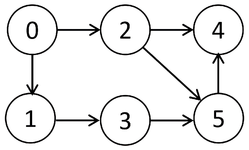
Two illustrative examples are presented in this section to demonstrate the effectiveness of the proposed methods. First, we examine the advantage of protocol (8) in the first example. Then, we explore the AW compensation for MRS inputs in the second example. The communication topology used in this section is depicted in Figure 2.

5.1. Distributed Extended State Observer-Based Formation Control

An MAS comprising one leader and five followers is considered. The following are the system matrices
A = 0 1 0 0 0 1 4 6 4 , B = 0 1 0 1 1 0 , C = 1 0 0
with u 0 = K 0 x 0 and K 0 = 3.8569 5.3535 3.1976 0.0635 0.0341 0.7973 . This leads to an asymptotically stable closed-loop system x ˙ 0 = ( A + B K 0 ) x 0 , where
A + B K 0 = 0.0635 1.0341 0.7973 0.0635 0.0341 0.2027 0.1431 0.6465 0.8024
Thus, the leader’s input u 0 satisfies Assumption 3. The initial formation error is chosen to satisfy x c l ( 0 ) E ( P ¯ ) . The disturbances of the followers are chosen as w i ( t ) = [ 0.5 , 0.5 e ( 0.5 i ) t ] T , i = 1 , , 5 , which also satisfies Assumption 3. The TVF reference is
f i ( t ) = 10 sin ( t + 2 π ( i 1 ) / 5 ) 10 cos ( t + 2 π ( i 1 ) / 5 ) 10 sin ( t + 2 π ( i 1 ) / 5 ) , i = 1 , , 5
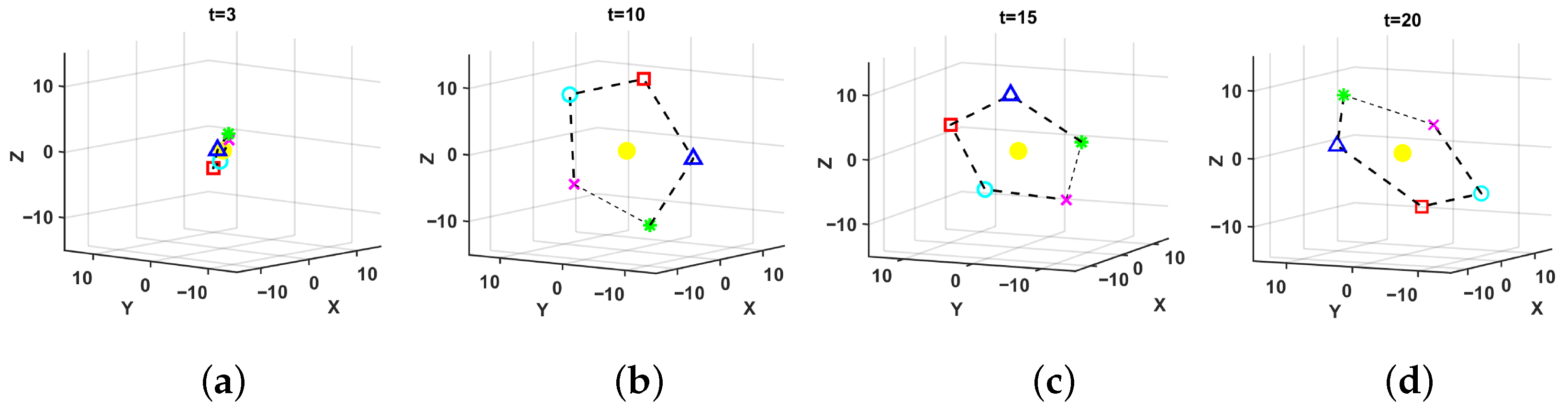
If the TVF is achieved, the five followers will be positioned at the vertices of a regular pentagon and rotate around the leader as the center. Let B ^ = 0 0 1 1 0 0 , B ˜ = 1 1 0 such that B ^ B = I 2 and B ˜ B = 0 ,. Then the feasibility condition (15) for formation is satisfied.
The control gain and observer gain obtained by Theorem 1 are
K 1 = 6.8838 10.2832 2.4213 4.5545 4.5962 8.5859 , L 1 = 0.2605 6.7171 7.1074 1.0956 5.8660 3.4955 , L 2 = 2.5955 1.7376 0.1820 3.0115
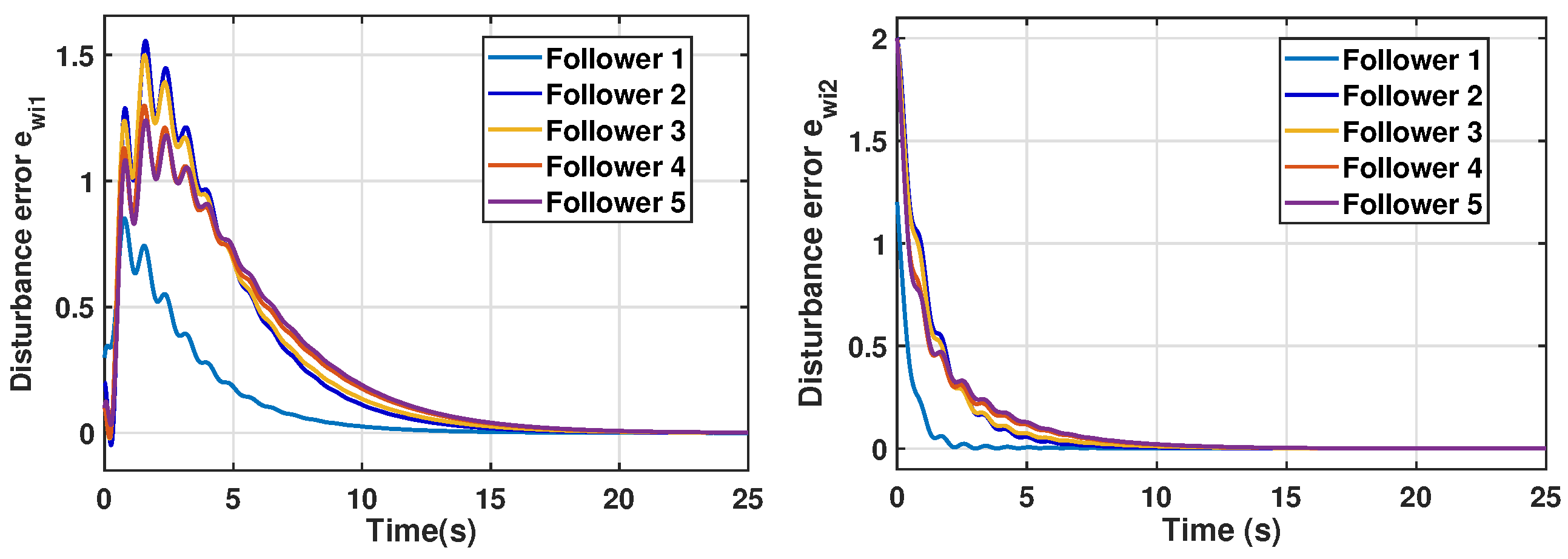
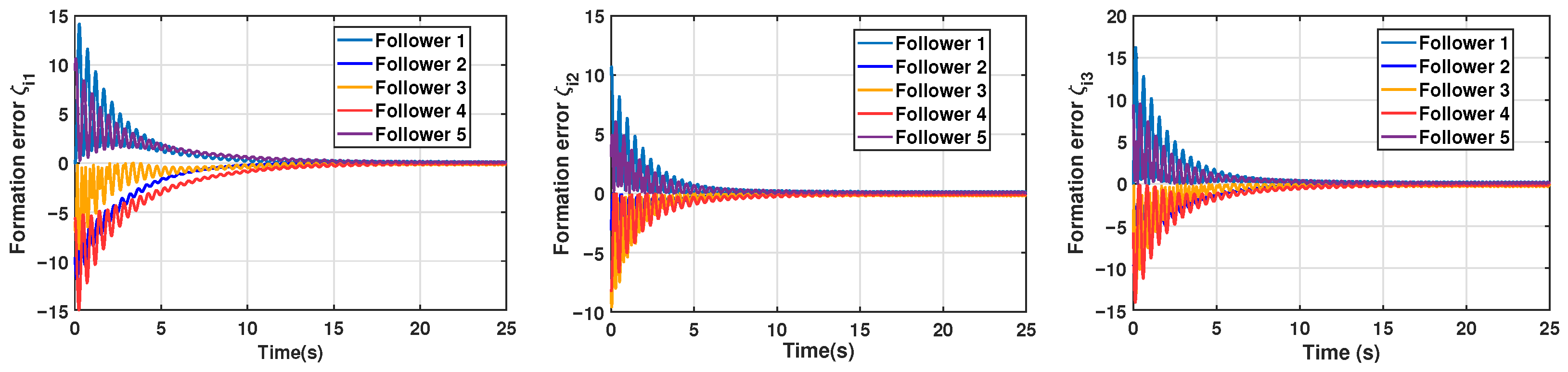
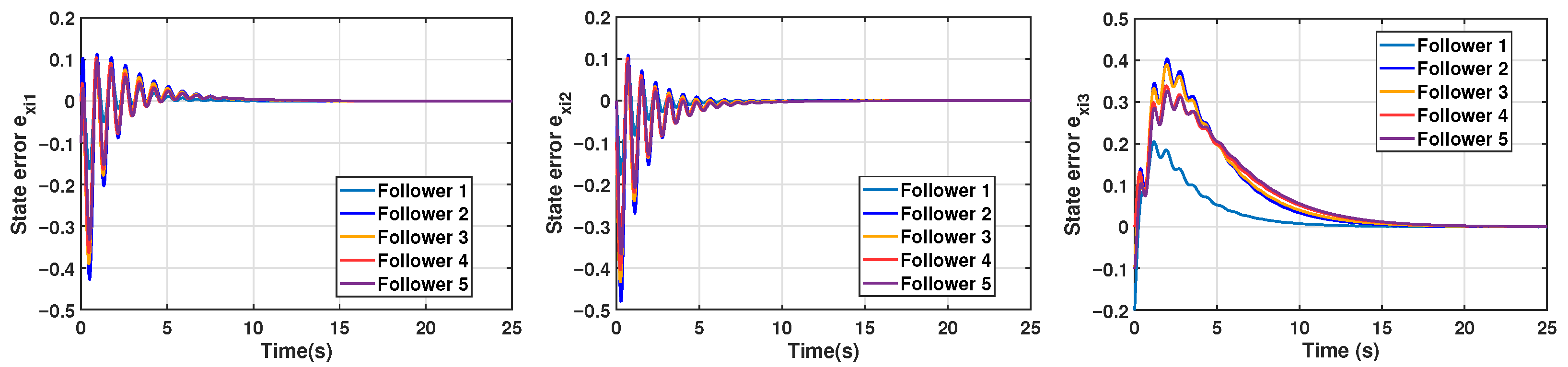
Figure 3 shows the states of the MAS at various time instances. As we can see, the followers successfully form a regular pentagon and track the leader toward the origin. Figure 4, Figure 5 and Figure 6 demonstrate that the TVF tracking errors and the estimation errors of the observers asymptotically converge, which demonstrated that the designed observers are effective.

5.2. Anti-Windup Formation Control with MRS

This section examines the AW compensation for the TVF tracking control of saturated MASs, where each follower is subject to MRS, with m = 2 and r = 25 . We consider an MAS composed of second-order agents
A = 0 1 1 0 , B = 0 1 , C = 1 0
with u 0 = K 0 x 0 and K 0 = 0 1 ; therefore, x ˙ 0 = ( A + B K 0 ) x 0 , where
A + B K 0 = 0 1 1 1
It is straightforward to have that the leader’s input u 0 satisfies Assumption 3. The disturbances are the same as in the first example. The formation reference signal is
f i ( t ) = 5 cos ( t + 2 π ( i 1 ) / 5 ) 5 sin ( t + 2 π ( i 1 ) / 5 )
The control gain and observer gain obtained through Theorem 1 are
K 1 = 0.4040 1.2120 , L = 1.3451 2.0955 0.9355
Following the obtained controller, the AW gains through Theorem 2 with α = 2 are
Δ m = 0.2078 4.6343 0.2937 0.0291 T , Δ r = 0.5816 .
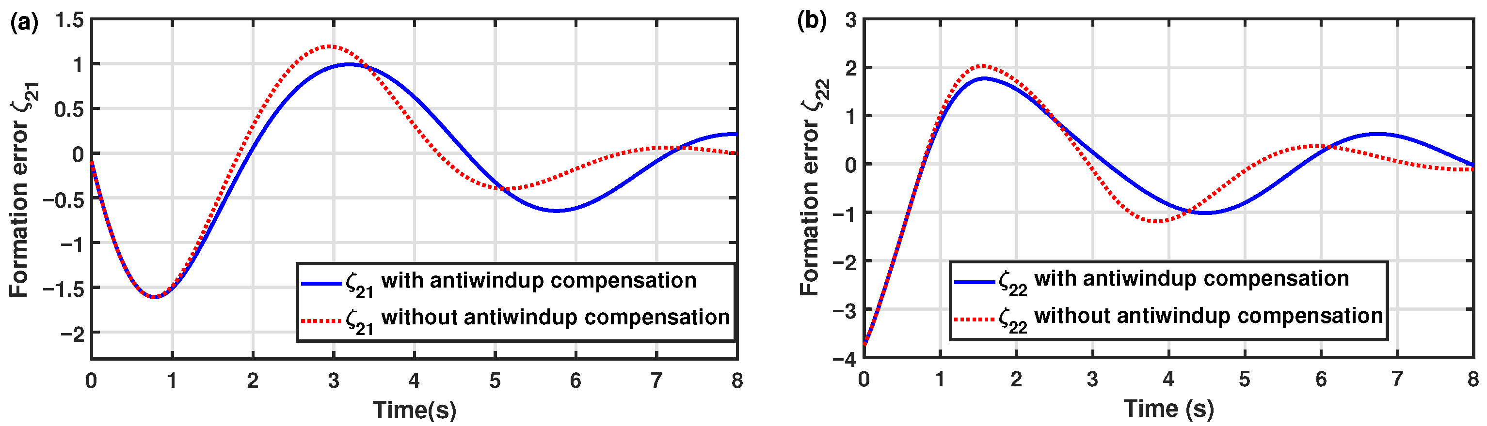
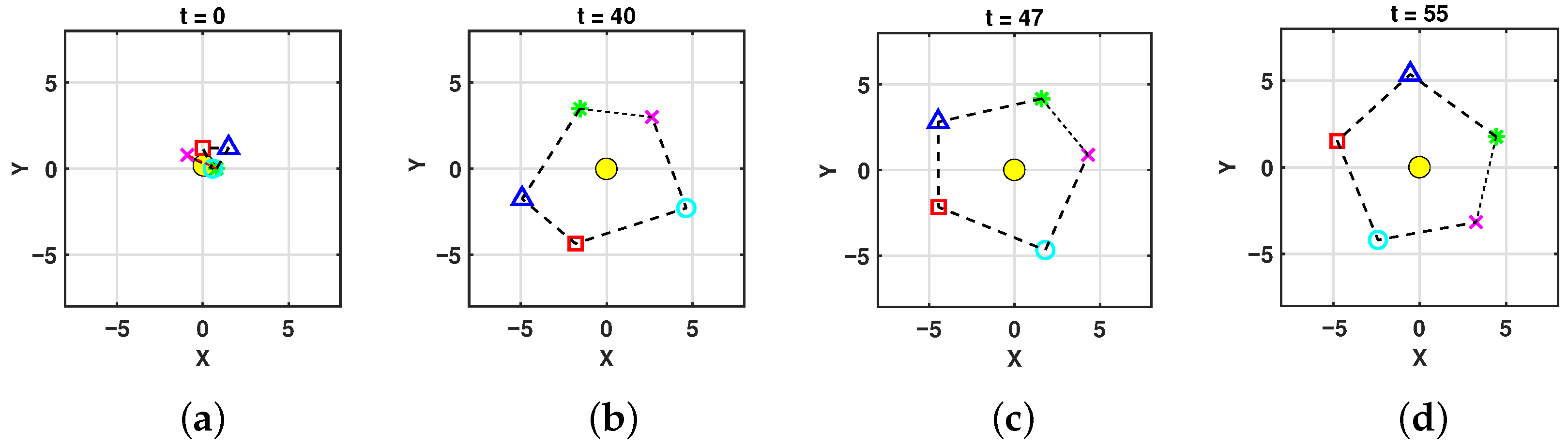
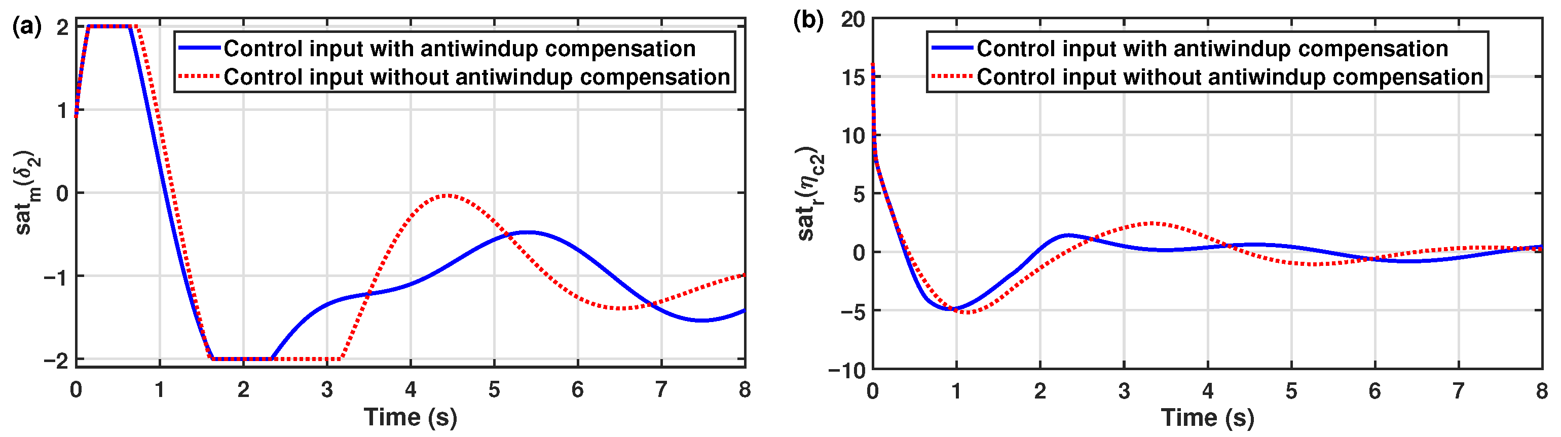
Figure 7 presents the states of the leader and followers at various time instants. For generality and without loss of scope, agent 2 is selected to demonstrate the compensation performance. To satisfy the initial constraint in Theorem 2, we set x c l ( 0 ) E ( P ¯ ) . The signals after MRS function are depicted in Figure 8, where the solid line represents the signal with AW compensation, and the dotted line is without AW compensation. As is illustrated in Figure 8a, the control input with anti-windup compensation exits the saturation region faster, and its rate is also reduced as shown in Figure 8b. Figure 9 shows that the TVF tracking errors with anti-windup compensation have smaller overshoot. The first component of the tracking error is reduced from 1.25 to 1 by 20%. Thus, this example demonstrates the effectiveness of the anti-windup design in dealing with MRS.
The simulations in Section 5 were executed on a Dell OptiPlex 7080 desktop with an Intel i7-10700 CPU and 16 GB RAM, using MATLAB R2022b.

6. Conclusions

This paper studies the leader-following TVF control problem for general linear MASs under MRS conditions, where the leader is driven by a nonzero control input and the followers are affected by unknown external disturbances. The leader’s input and the unknown disturbances of followers are treated as new states, and estimated by a distributed ESO, which incorporates an output feedback controller to guarantee the asymptotic convergence of TVF errors. To mitigate the MRS impacts, a static AW compensation is designed for followers, and the AW problem is solved by formulating an optimization problem. The future work is to consider the formation control of nonlinear MASs with MRS.

Author Contributions

Methodology, P.L.; Software, Z.L.; Writing—original draft, P.L.; Writing—review & editing, Z.L. and K.W.; Supervision, P.L. and K.W. All authors have read and agreed to the published version of the manuscript.

Funding

This work was supported by the National Natural Science Foundation of China under Grant 62303086 and Grant 62503073, and the China Postdoctoral Science Foundation under Grant 2023M730460.

Institutional Review Board Statement

Not applicable.

Informed Consent Statement

Not applicable.

Data Availability Statement

The original contributions presented in this study are included in the article. Further inquiries can be directed to the corresponding author.

Conflicts of Interest

The authors state that there are no competing financial interests or personal relationships that could have influenced the research reported in this paper.

References

  1. Ribichini, G.; Frazzoli, E. Efficient coordination of multiple-aircraft systems. In 42nd IEEE International Conference on Decision and Control (IEEE Cat. No.03CH37475); IEEE: New York City, NY, USA, 2003; Volume 1, pp. 1035–1040. [Google Scholar]
  2. Ren, W.; Beard, R.W. Distributed Consensus in Multi-Vehicle Cooperative Control; Springer: London, UK, 2008; Volume 27. [Google Scholar]
  3. Su, Y.; Huang, J. Cooperative output regulation of linear multi-agent systems. IEEE Trans. Autom. Control 2011, 57, 1062–1066. [Google Scholar]
  4. Nigam, N.; Bieniawski, S.; Kroo, I.; Vian, J. Control of multiple UAVs for persistent surveillance: Algorithm and flight test results. IEEE Trans. Control Syst. Technol. 2011, 20, 1236–1251. [Google Scholar] [CrossRef]
  5. Li, Z.; Liu, X.; Ren, W.; Xie, L. Distributed tracking control for linear multiagent systems with a leader of bounded unknown input. IEEE Trans. Autom. Control 2012, 58, 518–523. [Google Scholar] [CrossRef]
  6. Dong, X.; Li, Q.; Wang, R.; Ren, Z. Time-varying formation control for second-order swarm systems with switching directed topologies. Inf. Sci. 2016, 369, 1–13. [Google Scholar] [CrossRef]
  7. Fathian, K.; Summers, T.H.; Gans, N.R. Robust distributed formation control of agents with higher-order dynamics. IEEE Control Syst. Lett. 2018, 2, 495–500. [Google Scholar] [CrossRef]
  8. Dong, X.; Li, Q.; Ren, Z.; Zhong, Y. Formation-containment control for high-order linear time-invariant multi-agent systems with time delays. J. Frankl. Inst. 2015, 352, 3564–3584. [Google Scholar] [CrossRef]
  9. Li, B.; Riaz, S.; Saleem, O.; Zhao, Y.; Iqbal, J. PD-type iterative learning consensus control approach for an electromechanical actuator-based multiagent system. Appl. Intell. 2025, 55, 684. [Google Scholar] [CrossRef]
  10. Dong, X.; Xi, J.; Lu, G.; Zhong, Y. Formation control for high-order linear time-invariant multiagent systems with time delays. IEEE Trans. Control Netw. Syst. 2014, 1, 232–240. [Google Scholar] [CrossRef]
  11. Dong, X.; Hu, G. Time-varying formation control for general linear multi-agent systems with switching directed topologies. Automatica 2016, 73, 47–55. [Google Scholar] [CrossRef]
  12. Dong, X.; Hu, G. Time-varying formation tracking for linear multiagent systems with multiple leaders. IEEE Trans. Autom. Control 2017, 62, 3658–3664. [Google Scholar] [CrossRef]
  13. Peng, X.; He, Y.; Shen, J. Time-varying formation tracking control of multi-leader multiagent systems with sampled-data. IEEE Trans. Autom. Sci. Eng. 2023, 21, 3182–3192. [Google Scholar] [CrossRef]
  14. Liu, Y.; Dong, X.; Li, Q.; Ren, Z.; Shi, P.; Yu, J. Robust time-varying output formation tracking for heterogeneous multi-agent systems with adaptive event-triggered mechanism. J. Frankl. Inst. 2022, 359, 5842–5864. [Google Scholar]
  15. Lu, Y.; Dong, X.; Li, Q.; Lü, J.; Ren, Z. Time-varying group formation-containment tracking control for general linear multiagent systems with unknown inputs. IEEE Trans. Cybern. 2021, 52, 11055–11067. [Google Scholar] [CrossRef]
  16. Zhang, X.; Wu, J.; Zhan, X.; Han, T.; Yan, H. Observer-based adaptive time-varying formation-containment tracking for multiagent system with bounded unknown input. IEEE Trans. Syst. Man Cybern. Syst. 2022, 53, 1479–1491. [Google Scholar] [CrossRef]
  17. Ouyang, Q.; Wu, Z.; Cong, Y.; Wang, Z. Formation control of unmanned aerial vehicle swarms: A comprehensive review. Asian J. Control 2023, 25, 570–593. [Google Scholar] [CrossRef]
  18. Li, J.; Dong, X.; Yu, J.; Li, Q.; Ren, Z. Resilient time-varying formation tracking for heterogeneous high-order multiagent systems with multiple dynamic leaders. IEEE Trans. Control Netw. Syst. 2023, 11, 89–100. [Google Scholar] [CrossRef]
  19. Li, J.; Hua, Y.; Yu, J.; Dong, X.; Feng, Z.; Ren, Z. Resilient time-varying formation tracking control for general linear multiagent systems with a nonautonomous leader and adversarial followers. IEEE Trans. Cybern. 2024, 54, 6203–6216. [Google Scholar] [CrossRef]
  20. Huang, J.; Xie, J.; Huang, J.; Liu, S. Prescribed-time, event-triggered, adaptive, fault-tolerant formation control of heterogeneous air–ground multi-agent systems under deception attacks and actuator faults. Actuators 2025, 14, 575. [Google Scholar] [CrossRef]
  21. Hua, Y.; Dong, X.; Li, Q.; Ren, Z. Distributed time-varying formation robust tracking for general linear multiagent systems with parameter uncertainties and external disturbances. IEEE Trans. Cybern. 2017, 47, 1959–1969. [Google Scholar] [CrossRef]
  22. Zhang, S.; Li, Z.; Wang, X. Robust H2 consensus for multi-agent systems with parametric uncertainties. IEEE Trans. Circuits Syst. II Express Briefs 2021, 68, 2473–2477. [Google Scholar]
  23. Yan, B.; Shi, P.; Lim, C.; Wu, C. Robust formation control for multiagent systems based on adaptive observers. IEEE Syst. J. 2021, 16, 3139–3150. [Google Scholar] [CrossRef]
  24. Chen, J.; Shi, Z.; Zhong, Y. Robust formation tracking for uncertain multi-agent systems with unknown leader input. IET Control Theory Appl. 2020, 14, 646–653. [Google Scholar] [CrossRef]
  25. Cheng, J.; Kang, Y.; Xin, B.; Zhang, Q.; Mao, K.; Zhou, S. Time-varying trajectory tracking formation H control for multiagent systems with communication delays and external disturbances. IEEE Trans. Syst. Man Cybern. Syst. 2021, 52, 4311–4323. [Google Scholar] [CrossRef]
  26. Wang, Q.; Dong, X.; Wang, B.; Hua, Y.; Ren, Z. Finite-time observer-based H fault-tolerant output formation tracking control for heterogeneous nonlinear multi-agent systems. IEEE Trans. Netw. Sci. Eng. 2023, 10, 1822–1834. [Google Scholar] [CrossRef]
  27. Peng, X.; He, Y.; Liu, Z.; You, L.; Li, H. Time-varying formation H tracking control and optimization for delayed multi-agent systems with exogenous disturbances. IEEE Trans. Autom. Sci. Eng. 2024, 22, 5637–5647. [Google Scholar] [CrossRef]
  28. Cao, W.; Zhang, J.; Ren, W. Leader–follower consensus of linear multi-agent systems with unknown external disturbances. Syst. Control Lett. 2015, 82, 64–70. [Google Scholar] [CrossRef]
  29. Qin, W.; Liu, Z.; Chen, Z. Formation control for nonlinear multi-agent systems with linear extended state observer. IEEE/CAA J. Autom. Sin. 2014, 1, 171–179. [Google Scholar] [CrossRef]
  30. Liu, A.; Zhang, W.; Yu, L.; Yan, H.; Zhang, R. Formation control of multiple mobile robots incorporating an extended state observer and distributed model predictive approach. IEEE Trans. Syst. Man Cybern. Syst. 2018, 50, 4587–4597. [Google Scholar] [CrossRef]
  31. Yu, J.; Dong, X.; Liang, Z.; Li, Q.; Ren, Z. Practical time-varying formation tracking for high-order nonlinear multiagent systems with multiple leaders based on the distributed disturbance observer. Int. J. Robust Nonlinear Control 2018, 28, 3258–3272. [Google Scholar] [CrossRef]
  32. Wang, L.; Xi, J.; He, M.; Liu, G. Robust time-varying formation design for multiagent systems with disturbances: Extended state-observer method. Int. J. Robust Nonlinear Control 2020, 30, 2796–2808. [Google Scholar] [CrossRef]
  33. Li, Z.; Zhao, Y. Active disturbance rejection formation tracking control for uncertain nonlinear multi-agent systems with switching topology via dynamic event-triggered extended state observer. IEEE Trans. Circuits Syst. I Regul. Pap. 2022, 70, 518–529. [Google Scholar] [CrossRef]
  34. Wu, Y.; Liang, H.; Xuan, S.; Zhang, X. Extended state observer based finite-time fault-tolerant formation control for multi-uavs. J. Frankl. Inst. 2024, 361, 107158. [Google Scholar] [CrossRef]
  35. Yang, Y.; Yang, T.; Zhou, S.; Sun, W.; Wu, D. Prescribed-time extended state observer-based bipartite formation control of vehicle multi-agent systems. IEEE Trans. Autom. Sci. Eng. 2024, 22, 2174–2185. [Google Scholar] [CrossRef]
  36. Wang, J.; Wang, C.; Wei, Y.; Zhang, C. Observer-based neural formation control of leader–follower AUVs with input saturation. IEEE Syst. J. 2020, 15, 2553–2561. [Google Scholar] [CrossRef]
  37. Liu, F.; Hua, Y.; Dong, X.; Li, Q.; Ren, Z. Adaptive fault-tolerant time-varying formation tracking for multi-agent systems under actuator failure and input saturation. ISA Trans. 2020, 104, 145–153. [Google Scholar] [CrossRef] [PubMed]
  38. Zhang, X.; Wu, J.; Zhan, X.; Han, T.; Yan, H. Adaptive time-varying formation tracking for multi-agent systems with input saturation via low-gain feedback approach. Trans. Inst. Meas. Control 2023, 45, 1079–1088. [Google Scholar] [CrossRef]
  39. Zhang, X.; Zhan, X.; Wu, J.; Han, T.; Yan, H. Distributed adaptive time-varying formation tracking for input saturated multi-agent systems with multiple leaders. IEEE Trans. Circuits Syst. II Express Briefs 2023, 71, 2084–2088. [Google Scholar] [CrossRef]
  40. Li, X.; Wu, J.; Zhan, X.; Cheng, L.; Wu, B. Distributed adaptive time-varying formation tracking for directed multi-agent systems subject to saturated-input with active leader. Int. J. Control. Autom. Syst. 2025, 23, 1082–1091. [Google Scholar] [CrossRef]
  41. Yu, J.; Dong, X.; Han, L.; Li, Q.; Ren, Z. Practical time-varying output formation tracking for high-order nonlinear strict-feedback multi-agent systems with input saturation. ISA Trans. 2020, 98, 63–74. [Google Scholar] [CrossRef]
  42. Park, B.S.; Yoo, S.J. Time-varying formation control with moving obstacle avoidance for input-saturated quadrotors with external disturbances. IEEE Trans. Syst. Man Cybern. Syst. 2024, 54, 3270–3282. [Google Scholar] [CrossRef]
  43. Yu, L.; Li, P.; Sun, X. Robust output constrained control for uncertain nonlinear systems subject to magnitude and rate saturation: Application to aircraft engine. IEEE Trans. Ind. Inform. 2020, 17, 6044–6053. [Google Scholar] [CrossRef]
  44. Yu, L.; Sun, X.; Gao, Y. Active disturbance rejection control for uncertain nonlinear systems subject to magnitude and rate saturation: Application to aeroengine. IEEE Trans. Syst. Man Cybern. Syst. 2021, 52, 2201–2212. [Google Scholar] [CrossRef]
  45. Zhou, P.; Chen, B. Semi-global leader-following output consensus of heterogeneous systems subject to actuator position and rate saturation. Auton. Intell. Syst. 2021, 1, 8. [Google Scholar] [CrossRef]
  46. Li, P.; Jabbari, F.; Sun, X. Leader–follower consensus of linear multiagent systems with magnitude and rate saturation and an active leader. IEEE Trans. Autom. Control 2022, 68, 5584–5591. [Google Scholar] [CrossRef]
  47. Xia, G.; Xia, X.; Zheng, Z. Formation tracking control for underactuated surface vehicles with actuator magnitude and rate saturations. Ocean Eng. 2022, 260, 111935. [Google Scholar] [CrossRef]
  48. Liang, K.; Cui, J.; Lu, P.; Chen, Y.; Lin, X.; Sun, Y.; Zhang, Q.; Wen, X.; Duan, Y. Minimal learning parameters-based simplified robust adaptive saturated control for dynamic positioning ship with input magnitude and rate saturations. Ocean Eng. 2024, 297, 117032. [Google Scholar] [CrossRef]
  49. Da Silva, J.G.; Tarbouriech, S. Antiwindup design with guaranteed regions of stability: An LMI-based approach. IEEE Trans. Autom. Control 2005, 50, 106–111. [Google Scholar] [CrossRef]
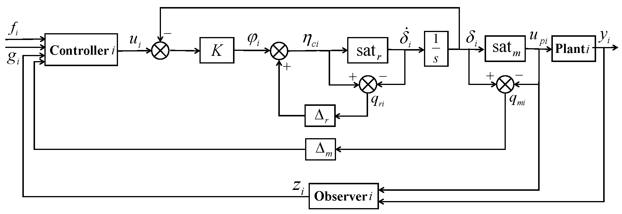
Figure 1. Anti-windup design for saturated agent i.
Actuators 15 00110 g001
Figure 2. The communication graph used in this section.
Actuators 15 00110 g002
Figure 3. State snapshots of the leader and five followers at selected time instants (a) t = 3 s; (b) t = 10 s; (c) t = 15 s; (d) t = 20 s.
Actuators 15 00110 g003
Figure 4. The TVF tracking errors.
Actuators 15 00110 g004
Figure 5. Followers’ disturbance estimation errors.
Actuators 15 00110 g005
Figure 6. Followers’ state estimation errors.
Actuators 15 00110 g006
Figure 7. State snapshots of the leader and five followers at selected time instants (a) t = 0 s; (b) t = 40 s; (c) t = 47 s; (d) t = 55 s.
Actuators 15 00110 g007
Figure 8. The saturated control input of agent 2.
Actuators 15 00110 g008
Figure 9. The TVF tracking error of agent 2.
Actuators 15 00110 g009
Disclaimer/Publisher’s Note: The statements, opinions and data contained in all publications are solely those of the individual author(s) and contributor(s) and not of MDPI and/or the editor(s). MDPI and/or the editor(s) disclaim responsibility for any injury to people or property resulting from any ideas, methods, instructions or products referred to in the content.