Multi-Valve Coordinated Disturbance Rejection Control for an Intake Pressure System Using External Penalty Functions

Abstract

Altitude test facilities for aero-engines employ multi-chamber, multi-valve intake systems that require effective decoupling and strong disturbance rejection during transient tests. This paper proposes a coordinated active disturbance rejection control (ADRC) scheme based on external penalty functions. The chamber pressure safety limit is formulated as an inequality-constrained optimization problem, and an exponential penalty together with a gradient based algorithm is designed for dynamic constraint relaxation, with guaranteed global convergence. A coordination term is then integrated into a distributed ADRC framework to yield a multi-valve coordinated ADRC controller, whose asymptotic stability is established via Lyapunov theory. Hardware-in-the-loop simulations using MATLAB/Simulink and a PLC demonstrate that, under ±3 kPa pressure constraints, the maximum engine inlet pressure error is 1.782 kPa (77.1% lower than PID control), and under an 80 kg/s² flow-rate disturbance, valve oscillations decrease from ±27% to ±5%. These results confirm the superior disturbance rejection and decoupling performance of the proposed method.

1. Introduction

High-altitude simulation testing is the most efficient way to design, explore performance and characteristics, improve designs, tackle technical challenges, and reproduce or resolve faults in aero-engine development. A key issue in such tests is accurately emulating the in-flight environment. The inlet pressure control subsystem of the flight environment simulator is one of the core components of altitude test facilities [1,2,3,4,5]. Under transient conditions—such as thrust surges, inertial starts, and acceleration/deceleration—a pressure regulation system must deliver high dynamic performance and stability. This is essential to meet strict requirements on response speed, overshoot, and steady-state error in high-altitude bench tests [6,7].

Current research on high-flow aero-engine inlet systems focuses on three main aspects. First, robust disturbance rejection: during high-altitude tests, inlet flow can fluctuate violently (with rates exceeding 60 kg/s²). The system’s characteristics change accordingly, demanding control strategies that maintain excellent dynamic response and disturbance suppression over a wide disturbance range. Second, valve group coordination: most existing solutions design independent ADRC or PID controllers for each valve. They lack mechanisms that exploit inter-valve coupling, which limits overall scheduling efficiency and coordination. Third, constraint satisfaction: traditional methods rely on empirical tuning and do not embed systematic mathematical constraints or optimization analysis. This makes it hard to guarantee that all chamber pressures remain within predefined error bounds.

Therefore, a high-efficiency control architecture is required to meet the complex demands of high-flow, multi-chamber, multi-valve inlet systems in high-altitude simulation tests, integrating robust disturbance rejection, multi-valve coordination, and constraint-aware optimization.

A high-flow inlet system typically comprises several coupled chambers and multiple regulating valves. To distribute large volumes of airflow accurately in short timeframes, the valves must act in concert. However, the strong coupling among valves poses a multivariable decoupling challenge: the pressure wave generated by one valve affects not only its local chamber but also adjacent chambers. Nonlinear, time-varying dynamics, valve hysteresis, engine combustion instabilities, and random disturbances further complicate control design [8,9,10].

To address multi-actuator coordination, researchers have proposed various methods. Reference [11] uses linear matrix inequalities (LMIs) for flow allocation among valves, achieving coordinated control. In reference [12], a combination of open-loop and closed-loop control decouples and coordinates multiple valves. Reference [13] introduces a multimodal switching framework that blends adaptive sliding-mode control (ASMC) with disturbance observers (DOB). This approach switches between compensation and reset modes to mitigate image degradation in telescope scanning systems, using adaptive laws to suppress sliding-mode chattering. Although these methods demonstrate favorable results in their respective simulation environments, they generally require high linearity and limited uncertainty in the plant model—conditions not met by the highly nonlinear, strongly disturbed, large-scale MIMO inlet-pressure system.

The inlet-environment pressure control problem can be recast as a constrained optimization problem. Among the solution techniques, penalty-function methods transform constrained problems into unconstrained ones by incorporating constraint violations into the objective, thereby simplifying the solution process [14,15,16]. Penalty functions have been widely applied in aerospace control applications. In fixed-wing low-altitude flight, they handle aerodynamic constraints, attitude limits, and dynamic environment restrictions to enhance safety, stability, and efficiency. For unmanned aerial vehicles (UAVs), adaptive penalty-function methods optimize flight parameters under payload and endurance constraints, improving operational safety [17]. In UAV obstacle-avoidance research [18], penalty-function-defined safe regions boost flight safety in uncertain environments. Similarly, the inlet-pressure control task seeks to keep each chamber’s pressure within a prescribed error bound while minimizing simulation deviation, which can be cast as a constrained optimization problem and solved via a penalty-function approach.

Cooperative control denotes the process by which multiple subsystems work together toward a shared objective [19,20,21]. In current multi-chamber, multi-valve (MCMV) control systems, the chamber pressure is controlled independently: when a chamber has multiple regulating valves, individual valves are governed by separate single-input single-output (SISO) active disturbance rejection control (ADRC) controller. Although ADRC’s intrinsic decoupling endows the system with basic coordination [22,23,24,25], existing methods suffer from three major drawbacks. First, the sluggish dynamic response cannot accommodate rapid flow fluctuations, causing significant pressure overshoot. Second, without an active coordination mechanism to handle strong coupling among chambers and valves, the system—relying solely on ADRC’s passive decoupling—is prone to pressure oscillations under complex disturbances. Third, the control architecture grows linearly with valve count, leading to an exponential rise in tuning complexity and severely restricting practical deployment. Therefore, deeply integrating ADRC advantages with cooperative control theory to develop a multivariable coordination algorithm for strongly coupled scenarios is the key to improving overall system performance.

Motivated by the foregoing, this paper proposes a penalty-function-based coordinated ADRC for multi-chamber inlet-pressure regulation. The main contributions are as follows:

• We propose a cooperative optimization algorithm based on penalty functions for pressure control in MVMC systems. The algorithm maintains the simulation deviation at the engine inlet within predefined limits. It also improves the stability of chamber pressure. The convergence of the algorithm is theoretically guaranteed.
• We develop a coordinated ADRC scheme to address the inefficiency of independent control loops, improving control efficiency and robustness. Closed-loop stability is rigorously analyzed.
• We implement a hardware-in-the-loop (HIL) simulation to compare the proposed method with classical PID control, demonstrating its feasibility and superiority.

The remainder of this paper is organized as follows. Section 2 presents the multi-chamber pressure-control problem, system-structure characteristics, and control challenges. Section 3 derives the coupled pressure–temperature differential equations for the chambers and the nonlinear dynamic model of the control valves. Section 4 formulates the multi-objective cooperative optimization problem via exterior penalty functions and establishes convergence proofs. Section 5 designs the coordinated ADRC with disturbance compensation and performs closed-loop stability analysis. Section 6 validates the proposed algorithm on a hardware-in-the-loop platform and compares results with traditional PID control. Finally, Section 6 concludes the study and discusses future research directions.

2. Problem Statement

As discussed in the Introduction, the high-flow multi-chamber multi-valve (MVMC) intake pressure system is characterized by strong nonlinearities, tight inter-valve coupling, and significant disturbance sensitivity. In this section, we present a detailed description of the system structure, performance specifications, and the associated control challenges that motivate the proposed solution.

Figure 1 shows a schematic of the MVMC intake pressure control system (where the direction of airflow is indicated by the arrows). The system comprises two chambers: V1 and V2. The pressure in V2, representing the engine inlet pressure, is regulated by a butterfly valve (Valve1) and a sleeve valve (Valve2). The pressure in V1, which serves as the upstream boundary for V2, is controlled by a butterfly valve (Valve_air). A supply system provides constant inlet pressure and temperature to V1, and Valve_air exhausts to the ambient environment.

Engine test specifications require that the simulated V2 pressure never deviate by more than ±3 kPa from its setpoint at any time during the intake environment simulation. This ensures high-fidelity replication under both steady and transient operating conditions. Meanwhile, to maintain the safe operation of the supply unit throughout the test, the pressure in V1 should remain within ±5 kPa of its target value.

To achieve these control objectives, the three valves must operate in a coordinated manner to match the flow across the system. However, when the engine bleed flow changes rapidly and significantly (e.g., up to 60 kg/s²), traditional single-loop control strategies often fail to achieve effective coordination. Simulations under such conditions reveal issues such as valve saturation, pressure oscillations, and control lag—none of which meet the requirements of modern high-altitude engine testing.

Moreover, the system exhibits strong nonlinear behavior due to valve hysteresis, dynamic flow-pressure coupling, and time-varying plant characteristics during transients. These nonlinearities undermine the effectiveness of linear control strategies and degrade both tracking performance and robustness.

Additionally, the two chambers are tightly coupled via shared flow paths and interacting pressure dynamics. Adjustments to one valve can produce unintended pressure disturbances in the adjacent chamber, leading to a multivariable decoupling challenge. Addressing this issue requires a coordinated multivariable control approach that surpasses conventional single-loop PID or ADRC designs.

3. Inlet-Air System Model

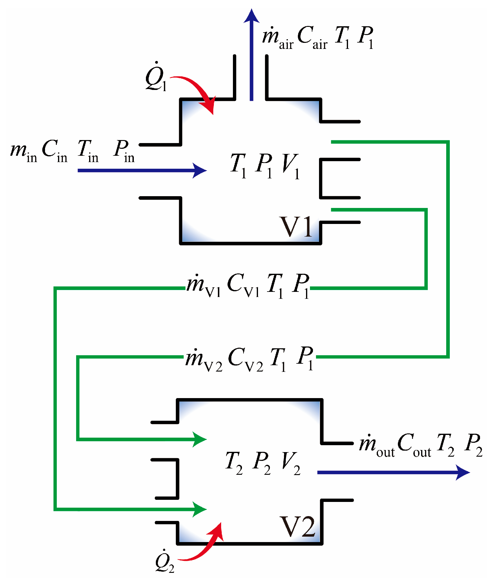
3.1. Chamber Temperature and Pressure Model

As shown in Figure 1, the V1 chamber has one inlet and three outlets, while the V2 chamber has two inlets and one outlet (see Figure 2). In the diagram, $\dot{m}$, $C$, $T$, $P$, $V$, $\dot{Q}$ denote the mass flow rate, mean flow velocity, temperature, pressure, chamber volume, and heat transfer rate between the chamber and its surroundings, respectively. The subscript “in” refers to the main supply manifold parameters; “air” to the flow parameters at Valve_air; “V1” and “V2” to those at Valve1 and Valve2; and “1” and “2” to the gas parameters in chambers V1 and V2, respectively.

Since the chamber volumes dominate the rates of pressure and temperature change and the connecting pipes are short, pipeline dynamics are neglected. Accordingly, a lumped parameter approach is used to model pressure and temperature dynamics in the stabilizing chambers. Defining control volumes 1 and 2 by the chamber walls and inlet/outlet boundaries and neglecting changes in potential energy, we derive the differential equations for pressure and temperature in V1 and V2 from the continuity equation, the energy equation, and the ideal gas law [8]:

$$\begin{array}{cc}{\displaystyle \frac{d{P}_1}{dt}}& ={\displaystyle \frac{R{T}_1}{V_1}}\left[{\dot{m}}_{in}-\left.\left({\dot{m}}_{air}+{\dot{m}}_1+{\dot{m}}_2\right)\right]\right.\hfill \\ & +{\displaystyle \frac{R}{V_1(C_p-R)}}\left[{\dot{Q}}_1+{\dot{m}}_{in}\left(h_{in}+{\displaystyle \frac{1}{2}}{C}_{in}^2\right)-{\dot{m}}_{air}\left(h_{air}+{\displaystyle \frac{1}{2}}{C}_{air}^2\right)\right.\hfill \\ & \left.-{\dot{m}}_1\left(h_1+{\displaystyle \frac{1}{2}}{C}_1^2\right)-{\dot{m}}_2\left(h_2+{\displaystyle \frac{1}{2}}{C}_2^2\right)-C_p{T}_1\left[{\dot{m}}_{\mathrm{in}}-\left({\dot{m}}_{air}+{\dot{m}}_1+{\dot{m}}_2\right)\right]\right]\hfill \end{array}$$

(1)

$$\begin{array}{cc}{\displaystyle \frac{d{T}_1}{dt}}& ={\displaystyle \frac{R{T}_1}{P_1{V}_1(C_p-R)}}\left[{\dot{Q}}_1+{\dot{m}}_{in}\left(h_{in}+{\displaystyle \frac{1}{2}}{C}_{in}^2\right)\right.-{\dot{m}}_{air}\left(h_{air}+{\displaystyle \frac{1}{2}}{C}_{air}^2\right)\hfill \\ & \left.-{\dot{m}}_1\left(h_1+{\displaystyle \frac{1}{2}}{C}_1^2\right)-{\dot{m}}_2\left(h_2+{\displaystyle \frac{1}{2}}{C}_2^2\right)-C_p{T}_1\left[{\dot{m}}_{in}-\left({\dot{m}}_{air}+{\dot{m}}_1+{\dot{m}}_2\right)\right]\right]\hfill \end{array}$$

(2)

$$\begin{array}{cc}{\displaystyle \frac{d{P}_2}{dt}}& ={\displaystyle \frac{R{T}_2}{V_2}}\left({\dot{m}}_1+{\dot{m}}_2-{\dot{m}}_{out}\right)+{\displaystyle \frac{R}{V_2(C_p-R)}}\left[{\dot{Q}}_1+{\dot{m}}_1\left(h_1+{\displaystyle \frac{1}{2}}{C}_1^2\right)\right.\hfill \\ & \left.+{\dot{m}}_2\left(h_2+{\displaystyle \frac{1}{2}}{C}_2^2\right)-{\dot{m}}_{out}\left(h_{out}+{\displaystyle \frac{1}{2}}{C}_{out}^2\right)-C_p{T}_2\left({\dot{m}}_1+{\dot{m}}_2-{\dot{m}}_{out}\right)\right]\hfill \end{array}$$

(3)

$$\begin{array}{cc}{\displaystyle \frac{d{T}_2}{dt}}& ={\displaystyle \frac{R{T}_2}{P_2{V}_2(C_p-R)}}\left[{\dot{Q}}_1+{\dot{m}}_1\left(h_1+{\displaystyle \frac{1}{2}}{C}_1^2\right)\right.+{\dot{m}}_2\left(h_2+{\displaystyle \frac{1}{2}}{C}_2^2\right)\hfill \\ & \left.-{\dot{m}}_{out}\left(h_{out}+{\displaystyle \frac{1}{2}}{C}_{out}^2\right)-C_p{T}_2\left({\dot{m}}_1+{\dot{m}}_2-{\dot{m}}_{out}\right)\right]\hfill \end{array}$$

(4)

In these expressions, $P_1$, $T_1$, $V_1$ and $T_2$, $P_2$, $V_2$ denote the pressure, temperature, and volume of chambers V1 and V2, respectively. The terms $h_{out}$, $h_{in}$, $h_1$, $h_2$, and $h_{air}$ are the specific enthalpies of the airflow at five sections: the outlet of V2, the inlet of V1, Valve1, Valve2, and Valve_air, respectively. ${\dot{Q}}_1$ and ${\dot{Q}}_2$ are the net rates of heat transfer between the V1 and V2 chambers and their surroundings, respectively. Finally, $C_P$ is the specific heat at a constant pressure, and R is the gas constant.

3.2. Control Valve Model

The intake pressure control system employs butterfly and sleeve valves with large diameters as flow-regulating elements. Both valve types are actuated by a hydraulic-servo closed loop control system. Consequently, the valve model includes a flow characteristic model and a dynamic characteristic model, as shown in Figure 3. In this figure, $V{P}_{\mathrm{cmd}}$ denotes the valve opening command, $A_{\mathrm{act}}$ denotes the actual equivalent flow area, and ${\dot{m}}_{\mathrm{out}}$ denotes the actual flow rate through the valve.

3.2.1. Valve Flow Characterization Models

The theoretical flow equations for butterfly and sleeve valves are complex and not convenient for practical use. Therefore, the flow coefficient method is adopted for modeling, and a generalized flow equation is used to characterize their flow characteristics [8], as follows:

$$\dot{m}=\phi Ap\sqrt{{\displaystyle \frac{2}{RT}}}$$

(5)

In this equation, $\dot{m}$ denotes the gas mass flow rate through the control valve; $\phi$ is the flow coefficient obtained by fitting experimental data; $\rho$ is the chamber gas density; A is the valve’s equivalent flow area; and $p$ and T are the upstream gas pressure and temperature, respectively. The coefficient $\phi$ depends on the upstream pressure $p$, downstream pressure $p_a$, and equivalent flow area A, as given below.

$$\phi =f\left(p,p_a,A\right)$$

(6)

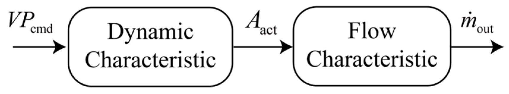
3.2.2. Control Valve Dynamic Characteristic Model

The valve plate is driven by a hydraulic cylinder through a linkage mechanism, and the spool displacement is controlled by a closed-loop negative-feedback system. With optimized controller parameters, the dynamic response of this displacement loop can be approximated as a first-order inertial process. Due to clearances between the valve plate and linkages, hysteresis arises during actuation. This is represented by a nonlinear function $f_{VP}$. The valve’s dynamic characteristic model is shown in Figure 4, where $\tau$ is the time constant.

4. Design of Pressure Coordination Control Algorithm Based on Penalty Function

4.1. Description of Optimization Problem

Based on the problem statement in Section 2, the control objectives of the intake pressure control system are to ensure that the pressures in chambers V1 and V2 track their setpoints or reject disturbances. The constraints impose bounds on the deviations between actual and preset pressures in V1 and V2. Therefore, the problem is cast as an optimization problem with inequality constraints:

$$\begin{array}{l}\min f\left(P_1,P_2\right)\\ s.t.g_i\left(P_1,P_2\right)\le 0\end{array}$$

(7)

where $f,g_i:R^n\to R,i\in \left\{1,2\right\}$ is a continuously differentiable function, and the feasible domain of problem (7) is $S=\left\{P_1,P_2\in R^n|g_i\left(P_1,P_2\right)\le 0,i\in \left\{1,2\right\}\right\}$.

4.2. Construction of Penalty Function

The penalty-function method converts a constrained optimization problem into an unconstrained one. It is a key approach for solving optimization problems with inequality constraints. Specifically, with target setpoints $P_{1\mathrm{set}}$ and $P_{2\mathrm{set}}$, the objective function $f\left(P_1,P_2\right)$ in the optimization problem is defined as

$$f\left(P_1,P_2\right)={\left(P_1-P_{1\mathrm{set}}\right)}^2+{\left(P_2-P_{2\mathrm{set}}\right)}^2$$

(8)

In addition, the valid simulation pressure range for the two chambers, $g_i\left(P_1,P_2\right)$, can be expressed as

$$\begin{array}{l}{g}_1\left(P_1,P_2\right)={\left(P_1-P_{1\mathrm{set}}\right)}^2-{\epsilon }_1^2\\ g_2\left(P_1,P_2\right)={\left(P_2-P_{2\mathrm{set}}\right)}^2-{\epsilon }_2^2\end{array}$$

(9)

where ${\epsilon }_1$ and ${\epsilon }_2$ represent the maximum allowable deviations from the setpoint pressures in chambers V1 and V2, respectively. Based on the above inequality constraints, the augmented objective function is defined as follows:

$$L\left(P_1,P_2,\mu \right)=f\left(P_1,P_2\right)+\gamma \alpha \left(P_1,P_2,\eta \right)$$

(10)

where $\gamma >0$ is the penalty factor, $\alpha \left(P_1,P_2,\eta \right)$ is the penalty function, and $\eta =[\mu ,\sigma ]>0$ is the tuning parameter. Based on the characteristics of the exponential function, the penalty function is designed as follows:

$$\alpha \left(P_1,P_2,\eta \right)={\displaystyle \sum _{i=1}^2{\left(e^{\max \left\{0,\eta g_i\left(P_1,P_2\right)\right\}}-1\right)}^2}$$

(11)

4.3. Design of Coordinated Optimization Control Algorithm

Based on the control objectives and the penalty function, the constrained problem can be transformed into

$$\underset{P_1,P_2}{\min }L\left(P_1,P_2,\gamma \right)$$

(12)

When the system reaches optimality, the augmented objective function attains its optimum values $\left\{P_1^{*},P_2^{*}\right\}=\arg \min L\left(P_1,P_2,\gamma \right)$. This ensures that both chamber pressures converge rapidly to their setpoints and remain within the prescribed error bounds throughout regulation. The algorithm is as elaborated follows:

• Step 1: Parameter Initialization

Initialize the state variables, $P_1,P_2$, and choose the initial penalty factor ${\gamma }_0$, tuning coefficient ${\eta }_0=[{\mu }_0,{\sigma }_0]$ and gradient learning rate $l$.

• Step 2: Iterative Process

(a) Construct the augmented objective function $L\left(P_1,P_2,\gamma \right)$ by adding penalty terms according to the constraints, then compute its gradient.

$$\nabla L\left(P_1,P_2,\gamma \right)={\left[{\displaystyle \frac{\partial L\left(P_1,P_2,\gamma \right)}{\partial P_1}},{\displaystyle \frac{\partial L\left(P_1,P_2,\gamma \right)}{\partial P_2}}\right]}^{\mathrm{T}}.$$

(b) Use a gradient-based optimization method to solve the penalized problem and obtain the solution at iteration $k$.

$$\underset{p_1,p_2}{\min }{L}_k\left(P_{1,k},P_{2,k},{\gamma }_k\right)$$

(13)

(c) Update the state variables.

$$\begin{array}{l}{P}_{1,k+1}=P_{1,k}-l\nabla L_k(P_{1,k},P_{2,k},{\gamma }_k)e_1\\ P_{2,k+1}=P_{2,k}-l\nabla L_k(P_{1,k},P_{2,k},{\gamma }_k)e_2\end{array}$$

(14)

where $e_1$ and $e_2$ denote the deviations of the chamber pressures from their preset values.

(d) Update the penalty coefficient ${\gamma }_{k+1}={\omega }_1{\gamma }_k$.

• Step 3: Termination Condition

Stop the iteration when either the solution $P_1,P_2$ converges within the required tolerance or the maximum number of iterations is reached. Additionally, if ${\gamma }_k\alpha (P_{1,k+1},P_{2,k+1},{\eta }_0)<\xi ,\xi >0$, terminate the algorithm.

4.4. Convergence Analysis

The existence of a feasible point is a prerequisite for the solvability of the optimization problem. This gives rise to the following lemma.

Lemma 1.

For any $\gamma >0,\eta =[\mu ,\sigma ]>0$ and $f\left(P_1,P_2\right)={\left(P_1-P_{1\mathrm{set}}\right)}^2+{\left(P_2-P_{2\mathrm{set}}\right)}^2$ suppose there exists $\left(P_1^{*},P_2^{*}\right)$ such that

$$\theta (\gamma )=\inf \{f(P_1,P_2)+\gamma \alpha (P_1,P_2,\eta )\}=L(P_1^{*},P_2^{*},\gamma )$$

(15)

Then

• (1) $\inf \{f(P_1,P_2)\mid g_i(P_1,P_2)\le 0\}\ge \sup \theta (\gamma )$
• (2) The penalty function $\alpha (P_1,P_2,\eta )$ is a nonincreasing function of $\gamma$, whereas both $f\left(P_1,P_2\right)$ and $\theta (\gamma )$ are nondecreasing in $\gamma$.

Proof of Lemma 1.

Consider a feasible point $\left(P_1,P_2\right)$ in the constraint set:

$$\begin{array}{l}S=\{P_1,P_2\in R^n\mid g_i(P_1,P_2)\le 0,i\in \{1,2\left\}\right\}\\ \alpha (P_1,P_2,\eta )={\displaystyle \sum _{i=1}^2{\left(e^{\max \{0,\eta g_i(P_1,P_2)\}}-1\right)}^2}=0\end{array}$$

(1) We have

$$\begin{array}{cc}f(P_1,P_2)& =f(P_1,P_2)+\gamma \alpha (P_1,P_2,\eta )\hfill \\ & \ge \inf \{f(P_1,P_2)+\gamma \alpha (P_1,P_2,\eta )\}\hfill \\ & =\theta (\gamma )\hfill \end{array}$$

Therefore, $\inf \{f(P_1,P_2)\mid g_i(P_1,P_2)\le 0\}\ge \sup \theta (\gamma ).$

• (2) According to the properties of $\theta (\gamma )$, assume $\gamma >{\gamma }^{\prime }$. Then we have

  $$f(P_1^{\prime },P_2^{\prime })+\gamma \alpha (P_1^{\prime },P_2^{\prime },\eta )\ge f(P_1,P_2)+\gamma \alpha (P_1,P_2,\eta )$$

  (16)

  $$f(P_1,P_2)+{\gamma }^{\prime }\alpha (P_1,P_2,\eta )\ge f(P_1^{\prime },P_2^{\prime })+{\gamma }^{\prime }\alpha (P_1^{\prime },P_2^{\prime },\eta ).$$

  (17)

  Adding these two inequalities yields $(\gamma -{\gamma }^{\prime })(\alpha (P_1^{\prime },P_2^{\prime },\eta )-\alpha (P_1,P_2,\eta ))\ge 0$, which implies that $\alpha (P_1,P_2,\eta )$ is nonincreasing in $\gamma$. □

From inequality (17), we also obtain $f(P_1,P_2)-f(P_1^{\prime },P_2^{\prime })\ge 0$; thus, $f\left(P_1,P_2\right)$ is nondecreasing in $\gamma$. Finally, inequality (17) further implies:

$$f(P_1,P_2)+{\gamma }^{\prime }\alpha (P_1,P_2,\eta )\ge f(P_1^{\prime },P_2^{\prime })+{\gamma }^{\prime }\alpha (P_1^{\prime },P_2^{\prime },\eta )=L(P_1^{\prime },P_2^{\prime },{\gamma }^{\prime })=\theta ({\gamma }^{\prime })$$

and

$$\theta (\gamma )+({\gamma }^{\prime }-\gamma )\alpha (P_1,P_2,\eta )\ge \theta ({\gamma }^{\prime }),$$

establishing that $\theta (\gamma )$ is nonincreasing in $\gamma$.

This completes the proof.

As $\gamma$ grows, the solution of the penalized problem diverges, and the value of L approaches the original objective function $f(P_1,P_2)$. This means that as the penalty for constraint violations becomes arbitrarily large, the solution increasingly approximates the global optimum of the original problem.

Theorem 1.

Any limit point of a convergent subsequence is a global optimal solution, and

$$\underset{\gamma \to +\infty }{\lim }L(P_1,P_2,\gamma )=f(P_1,P_2).$$

Proof of Theorem 1.

The proof details include three parts.

• (a) Boundedness of the penalty term
• Let

  $$\left(P_1^{*},P_2^{*}\right)=\arg {\min }_{P_1,P_2}L\left(P_1,P_2,\gamma \right).$$

  By Lemma 1,

  $$\begin{array}{ll}\inf \{f(p_c)\mid g_i(p_c)\le 0,h_i(p_c)-{\gamma }_i\le 0\}& \ge \theta (\mu ,\sigma )\hfill \\ & =f(p_c)+\mu \alpha (p_c)+\sigma \beta (p_c,{\gamma }_i)\hfill \\ & \ge f({p_c}^{*})+\mu \alpha ({p_c}^{*})+\sigma \beta ({p_c}^{*},{\gamma }_i)\hfill \\ & >f(p_c).\hfill \end{array}$$

  Since $\alpha (P_1,P_2,\eta )$ is nonincreasing in $\gamma$, it follows that

  $$f(P_1,P_2)-f(P_1^{*},P_2^{*})\le \gamma \alpha (P_1,P_2,\eta )\le \xi .$$

  Thus, $\alpha$ remains bounded as $\gamma$ grows.
• (b) Feasibility of the limit point
• As $\gamma \to +\infty$, both $\xi \to 0$ and $\alpha (P_1,P_2,\eta )\to 0$. For any convergent subsequence $\left\{P_{1,k},P_{2,k}\right\}$, Lemma 1 gives

  $$\begin{array}{cc}\underset{\gamma \ge 0}{\sup }\theta (\gamma )\ge \theta (\gamma ,k)& =f(P_1,P_2)+{\gamma }_k\alpha (P_1,P_2,\eta )\hfill \\ & \ge f(P_1,P_2)\hfill \end{array}$$

  Let $\left(P_1^{*},P_2^{*}\right)$ be its limit of $\left\{P_{1,k},P_{2,k}\right\}$, then

  $$\underset{\gamma \ge 0}{\sup }\theta (\gamma )\ge f(P_{1,k}^{*},P_{2,k}^{*}).$$

  Since

  $$\gamma \alpha (P_{1,k}^{*},P_{2,k}^{*},\eta )\to 0,$$

  $P_1^{*},P_2^{*}$ satisfies all original constraints of Problem (7).
• (c) Convergence of the augmented objective
• Again according to Lemma 1, $\left(P_1^{*},P_2^{*}\right)$ is an optimal solution and $\underset{\gamma \ge 0}{\sup }\theta (\gamma )=f(P_1^{*},P_2^{*}).$
• As $\gamma \to +\infty$,

  $$\gamma \alpha (P_1,P_2,\eta )=\theta (\gamma )-f(P_1,P_2)=f(P_1^{*},P_2^{*})-f(P_1^{*},P_2^{*})=0$$

  Therefore,

  $$\underset{\gamma \to +\infty }{\lim }L(P_1,P_2,\gamma )=f(P_1,P_2).$$

  □

5. Design of Cooperative Controller

Figure 5 shows the overall control framework. The dual-chamber intake system employs three independent control valves to achieve coordinated pressure regulation. To guarantee that the pressures in both chambers satisfy the prescribed error bounds throughout the control period, a coordinated ADRC based on the penalty function optimization algorithm presented in Section 3 is used. During operation, the algorithm parameters are iteratively updated based on the real-time system state. The optimization problem is then repeatedly solved until the pressure control objectives are met and stable convergence is achieved. In Figure 5, the blue region denotes the coordinated control algorithm; the green region, the primary controller; the yellow region, the decoupling module; the purple region, the simulation model; and the pink region, the extended state observer (ESO).

5.1. Pressure Control Model of Dual-Chamber System

The dual-chamber system considered in this study features large chamber volumes and relatively slow internal airflow. Additionally, temperature variations are limited during flight environment simulation tests. Therefore, the effects of gas kinetic energy and heat transfer between the airflow and pipeline walls are neglected in the control model. Based on this, and using Equations (1) and (3), the simplified state-space equations of chamber pressures with respect to ${\dot{m}}_{air},{\dot{m}}_1,{\dot{m}}_2$ are derived as follows:

$$\left[\begin{array}{c}{\dot{P}}_1\\ {\dot{P}}_2\end{array}\right]=\left[\begin{array}{ccc}-{\alpha }_1& -{\alpha }_2& -{\alpha }_{air}\\ {\beta }_1& {\beta }_2& 0\end{array}\right]\left[\begin{array}{c}{\dot{m}}_1\\ {\dot{m}}_2\\ {\dot{m}}_{air}\end{array}\right]+\left[\begin{array}{c}{f}_1\left(P_1,P_2\right)\\ f_2\left(P_1,P_2\right)\end{array}\right]$$

(18)

where

$${\alpha }_1={\displaystyle \frac{R}{V_1}}\left[T_1-{\displaystyle \frac{h_{in}-R{T}_1}{C_p-R}}\right],{\alpha }_2={\displaystyle \frac{R}{V_1}}\left[T_1-{\displaystyle \frac{h_2-R{T}_1}{C_p-R}}\right],{\alpha }_{air}={\displaystyle \frac{R}{V_1}}\left[T_1-{\displaystyle \frac{h_{air}-R{T}_1}{C_p-R}}\right],$$

$${\beta }_1={\displaystyle \frac{R}{V_2}}\left[T_2-{\displaystyle \frac{h_1-R{T}_2}{C_p-R}}\right],{\beta }_2={\displaystyle \frac{R}{V_2}}\left[T_2-{\displaystyle \frac{h_2-R{T}_2}{C_p-R}}\right].$$

$d_1\left(P_1,P_2\right)$ and $d_2\left(P_1,P_2\right)$ represent the total disturbances in the two pressure control systems, including factors such as the neglected heat transfer between airflow and pipelines, the inlet mass flow rate ${\dot{m}}_{in}$ into Chamber 1, and the engine extraction flow rate ${\dot{m}}_{out}$ from Chamber 2.

The control-valve position model shown in Figure 4 can be approximated by a first-order inertial element in series with an unobservable nonlinear element. By treating the nonlinear element as a disturbance and neglecting it, the transfer function from the valve-opening command to the valve flow can be written, based on Figure 4 and Equation (5), as follows:

$${\displaystyle \frac{{\dot{m}}_1}{V{P}_{1\mathrm{cmd}}}}={\displaystyle \frac{\pi }{4}}{D}_1^2{\phi }_1{P}_1\sqrt{{\displaystyle \frac{2}{R{T}_1}}}{\displaystyle \frac{1-\cos \left(V{P}_{1\mathrm{act}}\right)}{1+{\tau }_{1}s}}=G_1\left(s\right)$$

(19)

$${\displaystyle \frac{{\dot{m}}_2}{V{P}_{2\mathrm{cmd}}}}=K_{2}V{P}_{2\mathrm{act}}{\phi }_2{P}_1\sqrt{{\displaystyle \frac{2}{R{T}_1}}}{\displaystyle \frac{1}{1+{\tau }_{2}s}}=G_2\left(s\right)$$

(20)

$${\displaystyle \frac{{\dot{m}}_{air}}{V{P}_{air\mathrm{cmd}}}}={\displaystyle \frac{\pi }{4}}{D}_{air}^2{\phi }_{air}{P}_1\sqrt{{\displaystyle \frac{2}{R{T}_1}}}{\displaystyle \frac{1-\cos \left(V{P}_{air\mathrm{act}}\right)}{1+{\tau }_{air}s}}=G_{air}\left(s\right)$$

(21)

where $V{P}_{i\mathrm{act}}$, ${\phi }_i$, and ${\tau }_i$ denote the actual valve opening, flow coefficient, and actuator time constant of the control valve, respectively. The subscripts “air”, “1”, and “2” refer to Valve_air, Valve1, and Valve2, respectively. $D_i$ represents the valve diameter. For Valve2 (a sleeve valve), the flow area varies linearly with opening (i.e., $A_2=K_2\cdot V{P}_{2\mathrm{act}}$).

Substituting (19)–(21) into Equation (18) yields the simplified state-space equations:

$$\left[\begin{array}{c}{\dot{P}}_1\\ {\dot{P}}_2\end{array}\right]=\left[\begin{array}{ccc}{b}_{11}& b_{12}& b_{13}\\ b_{21}& b_{22}& 0\end{array}\right]\left[\begin{array}{c}V{P}_{1\mathrm{cmd}}\\ V{P}_{2\mathrm{cmd}}\\ V{P}_{air\mathrm{cmd}}\end{array}\right]+\left[\begin{array}{c}{d}_1\left(P_1,P_2\right)\\ d_2\left(P_1,P_2\right)\end{array}\right]$$

(22)

where

$$\begin{array}{l}{b}_{11}=-{\alpha }_1{G}_1\left(s\right),b_{12}=-{\alpha }_2{G}_1\left(s\right),b_{13}=-{\alpha }_{air}{G}_{air}\left(s\right)\\ b_{21}=-{\beta }_1{G}_1\left(s\right),b_{22}=-{\beta }_2{G}_2\left(s\right).\end{array}$$

Based on Equation (22), an affine model relating the three control inputs $u_1,u_2,u_{air}$ to the two chamber pressures is established as follows:

$$\left\{\begin{array}{c}{\ddot{P}}_1=b_{11}{u}_1+b_{12}{u}_2+b_{13}{u}_{air}+d_1\left(P_1,P_2\right)\hfill \\ {\ddot{P}}_2=b_{21}{u}_1+b_{22}{u}_2+d_2\left(P_1,P_2\right)\hfill \end{array}\right.$$

(23)

Define the matrix $\mathit{U}$ as the system’s virtual control input and the matrix $\mathit{B}$ as the system’s static coupling matrix:

$$\mathit{U}=\left[\begin{array}{c}{u}_{c1}\\ u_{c2}\end{array}\right]=\left[\begin{array}{ccc}{b}_{11}& b_{12}& b_{13}\\ b_{21}& b_{22}& 0\end{array}\right]\left[\begin{array}{c}{u}_1\\ u_2\\ u_{air}\end{array}\right]$$

(24)

$$\mathit{B}=\left[\begin{array}{c}{\mathit{B}}_{\mathbf{1}}\\ {\mathit{B}}_{\mathbf{2}}\end{array}\right]=\left[\begin{array}{ccc}{b}_{11}& b_{12}& b_{13}\\ b_{21}& b_{22}& 0\end{array}\right]$$

(25)

By introducing the virtual control vector,

$$\mathit{U}={\left[\begin{array}{cc}{u}_{c1}& u_{c2}\end{array}\right]}^{\mathrm{T}},$$

and the above equation can be reformulated as follows:

$$\left\{\begin{array}{c}{\ddot{P}}_1=u_{c1}+d_1\left(P_1,P_2\right)\\ {\ddot{P}}_2=u_{c2}+d_2\left(P_1,P_2\right)\end{array}\right.$$

(26)

Let $x_{11}=P_1$ and $x_{21}=P_2$; thus, we have

$$\left\{\begin{array}{c}{\dot{x}}_{11}=x_{12}\\ {\dot{x}}_{12}=u_{c1}+d_1\left(P_1,P_2\right)\\ y_1=x_{11}\end{array}\right.$$

(27)

$$\left\{\begin{array}{c}{\dot{x}}_{21}=x_{22}\\ {\dot{x}}_{22}=u_{c2}+d_2\left(P_1,P_2\right)\\ y_2=x_{21}\end{array}\right.$$

(28)

5.2. Design of Coordinated ADRC Controller

5.2.1. Design of ADRC

Construct ESO for the chamber pressure control systems V1 and V2 based on (27) and (28):

$$\left\{\begin{array}{c}{E}_1=z_{11}-y_1\\ {\dot{z}}_{11}=z_{12}-{\beta }_{11}{E}_1\\ {\dot{z}}_{12}=z_{13}-{\beta }_{12}{E}_1+u_{c1}\\ {\dot{z}}_{13}=-{\beta }_{13}{E}_1\end{array}\right.$$

(29)

$$\left\{\begin{array}{c}{E}_2=z_{21}-y_2\\ {\dot{z}}_{21}=z_{22}-{\beta }_{21}{E}_2\\ {\dot{z}}_{22}=z_{23}-{\beta }_{22}{E}_2+u_{c2}\\ {\dot{z}}_{23}=-{\beta }_{23}{E}_2\end{array}\right.$$

(30)

where

$$z_1=\left[\begin{array}{c}{z}_{11}\\ z_{12}\\ z_{13}\end{array}\right],z_2=\left[\begin{array}{c}{z}_{21}\\ z_{22}\\ z_{23}\end{array}\right]$$

are the state estimations for $P_1$ and $P_2$, respectively, and $z_{13}$ and $z_{23}$ denote the total disturbance estimations.

$${\beta }_1=\left[\begin{array}{c}{\beta }_{11}\\ {\beta }_{12}\\ {\beta }_{13}\end{array}\right],{\beta }_2=\left[\begin{array}{c}{\beta }_{21}\\ {\beta }_{22}\\ {\beta }_{23}\end{array}\right]$$

are the gain vectors for the two ESOs, respectively. The variable $e\left(t\right)$ represents the output state estimation error. Let ${\omega }_1$ and ${\omega }_2$ denote the observer bandwidths of the two ESOs. According to the bandwidth-based tuning method [23], the gain vectors can be selected as follows:

$$\begin{array}{l}{\beta }_{11}=3{\omega }_1,{\beta }_{12}=3{\omega }_1^2,{\beta }_{13}={\omega }_1^3\\ {\beta }_{21}=3{\omega }_2,{\beta }_{22}=3{\omega }_2^2,{\beta }_{23}={\omega }_2^3\end{array}$$

(31)

Assuming the linear extended state observer provides accurate estimations, the total disturbances acting on the system satisfy the following:

$$z_{13}\to d_1\left(P_1,P_2\right),z_{23}\to d_2\left(P_1,P_2\right).$$

(32)

Let $u_{c1}=u_{c1}^{*}-z_1$ and $u_{c2}=u_{c2}^{*}-z_2$. Based on Equation (32), Equations (27) and (28) can be reformulated as

$$\left\{\begin{array}{l}{\dot{x}}_{11}=x_{12}\hfill \\ {\dot{x}}_{12}=u_{c1}^{*}\hfill \\ y_1=x_{11}\hfill \end{array},\left\{\begin{array}{l}{\dot{x}}_{21}=x_{22}\hfill \\ {\dot{x}}_{22}=u_{c2}^{*}\hfill \\ y_2=x_{21}\hfill \end{array}\right..\right.$$

(33)

This transformation enables the observation and compensation of the total disturbance in the system, effectively reducing it to a cascade of second-order integrators controlled by $u_{ci}^{*}$.

By adopting a proportional-derivative (PD) controller as the core control strategy of ADRC, the resulting ADRC inputs can be expressed as

$$\begin{array}{l}{u}_{\mathrm{ADRC}\_1}=k_{11}\left(P_{1\mathrm{set}}-z_{11}\right)+k_{12}\left({\dot{P}}_{1\mathrm{set}}-z_{12}\right)-z_{13}\\ u_{\mathrm{ADRC}\_2}=k_{21}\left(P_{2\mathrm{set}}-z_{21}\right)+k_{22}\left({\dot{P}}_{2\mathrm{set}}-z_{22}\right)-z_{23}\end{array}$$

(34)

where $P_{1\mathrm{set}}$ and $P_{2\mathrm{set}}$ are the pressure setpoints for chambers V1 and V2, respectively, and ${\dot{P}}_{1\mathrm{set}}$ and ${\dot{P}}_{2\mathrm{set}}$ are obtained via a tracking differentiator (TD) [26]. The feedback gain matrix is $K=[K_1,K_2]$, where $K_1=\left[k_{11},k_{12}\right]$ and $K_2=\left[k_{21},k_{22}\right]$.

5.2.2. Design of Penalty-Function Based Coordinated ADRC

To ensure that the dual-chamber pressure dynamics possess strong disturbance rejection capabilities while simultaneously coordinating global cooperation and satisfying error-bound optimization constraints, the cooperative optimization algorithm proposed in Section 4 is introduced to construct the penalty-function-based coordinated ADRC scheme. This algorithm integrates the outputs of the ADRC controller with those of the cooperative optimization algorithm to guarantee both stable tracking of the target pressure values and enhanced disturbance rejection performance. The design of the algorithm is as follows:

$$\begin{array}{cc}{u}_{c1}& =u_{\mathrm{ADRC}\_1}+k_{13}\nabla L\left(P_1,P_2,\mu \right)\hfill \\ & =k_{11}\left(P_{1\mathrm{set}}-z_{11}\right)+k_{12}\left({\dot{P}}_{1\mathrm{set}}-z_{12}\right)+k_{13}\nabla L\left(P_1,P_2,\mu \right)-z_{13}\hfill \\ u_{c2}& =u_{\mathrm{ADRC}\_2}+k_{13}\nabla L\left(P_1,P_2,\mu \right)\hfill \\ & =k_{21}\left(P_{2\mathrm{set}}-z_{21}\right)+k_{22}\left({\dot{P}}_{2\mathrm{set}}-z_{22}\right)+k_{23}\nabla L\left(P_1,P_2,\mu \right)-z_{23}\hfill \end{array}$$

(35)

where $\nabla L\left(P_1,P_2,\mu \right)$ denotes the gradient of the cooperative optimization term, and $K_3=[k_{13},k_{23}]$ comprises the tuning parameters for this optimization control. The incorporation of the coordinated optimization term mathematically guarantees that the controlled pressure parameters of both chambers remain within the error boundaries throughout the control process.

5.3. Stability Analysis

In this section, the stability of the controller designed for the aforementioned control strategy is established. First, by combining the system model, the controller, and the observer, the closed-loop system is obtained as follows:

$$\left\{\begin{array}{l}\dot{x}(t)=A_{z}x(t)+B_{z}U(t)+L_f{f}_w,\hfill \\ \dot{z}(t)=A_{z}z(t)+B_{z}U(t)+L_{z}e(t),\hfill \\ {\dot{f}}_d(t)=L_{e}e(t),\hfill \\ \dot{e}(t)=L_f^{\mathrm{T}}[z(t)-\widehat{z}(t)]+L_{w}e(t).\hfill \end{array}\right.$$

(36)

where

$$\begin{array}{c}x(t)={\left[\begin{array}{cccc}{x}_{11}& x_{12}& x_{21}& x_{22}\end{array}\right]}^{\mathrm{T}},z(t)={\left[\begin{array}{cccc}{z}_{11}& z_{12}& z_{21}& z_{22}\end{array}\right]}^{\mathrm{T}},\\ f_d={\left[\begin{array}{cc}{f}_1& f_2\end{array}\right]}^{\mathrm{T}},f_d={\left[\begin{array}{cc}{z}_{13}& z_{23}\end{array}\right]}^{\mathrm{T}},e={\left[\begin{array}{cc}{e}_1& e_2\end{array}\right]}^{\mathrm{T}},\\ A_z=\left[\begin{array}{cccc}0& 1& 0& 0\\ 0& 0& 0& 0\\ 0& 0& 0& 1\\ 0& 0& 0& 0\end{array}\right],B_z=\left[\begin{array}{c}0\\ b_1\\ 0\\ b_2\end{array}\right],L_f=\left[\begin{array}{cc}0& 0\\ 1& 0\\ 0& 0\\ 0& 1\end{array}\right],L_z=\left[\begin{array}{cc}0& 0\\ -{\beta }_{12}& 0\\ 0& 0\\ 0& -{\beta }_{22}\end{array}\right],L_e=\left[\begin{array}{cc}-{\beta }_{13}& 0\\ 0& -{\beta }_{23}\end{array}\right],L_w=\left[\begin{array}{cc}-{\beta }_{11}& 0\\ 0& -{\beta }_{22}\end{array}\right].\end{array}$$

Define the augmented state vector:

$$\zeta (t)={[x^{\mathrm{T}}(t),z^{\mathrm{T}}(t),f_d^{\mathrm{T}}(t),e^{\mathrm{T}}(t)]}^{\mathrm{T}}$$

and substitute the controller into the plant. The closed-loop dynamics can be written as

$$\dot{\zeta }(t)=\mathbb{A}\zeta (t)+{\mathbb{B}}_w{f}_w(\zeta (t))+\mathbb{B}\nabla L(\zeta (t)).$$

(37)

with

$$\begin{array}{c}\mathbb{A}=\left[\begin{array}{cccc}{A}_z& B_{z}K& L_f& 0\\ 0& A_z+B_{z}K& 0& L_z\\ 0& 0& 0& L_e\\ L_f^{\mathrm{T}}& -L_f^{\mathrm{T}}& 0& 0\end{array}\right],\\ {\mathbb{B}}_w={[\begin{array}{cccc}{L}_f& 0& 0& 0\end{array}]}^{\mathrm{T}},\\ \mathbb{B}={[\begin{array}{cccc}-B_z{K}_3& -B_z{K}_3& 0& 0\end{array}]}^{\mathrm{T}}.\end{array}$$

We now establish stability of the closed-loop system.

Theorem 2.

Suppose the nonlinear external disturbance $f_w$ and the gradient $\nabla L(\xi (t))$ of the objective function are continuously differentiable and bounded and satisfy the sector bounds:

$$\begin{array}{l}{f}_w^{\mathrm{T}}{f}_w\le {\zeta }^{\mathrm{T}}M\xi \\ \nabla L^{\mathrm{T}}\nabla L\le {\zeta }^{\mathrm{T}}N\xi \end{array}$$

where M and N are positive-definite diagonal matrices characterizing the nonlinearities. If a symmetric positive-definite matrix P exists where

$$\begin{array}{c}\Gamma =\left[\begin{array}{cc}\vartheta & 2P\\ *& -I\end{array}\right]<0\\ \vartheta =P\mathbb{A}+{\mathbb{A}}^{\mathrm{T}}P+M+{\mathbb{B}}^{\mathrm{T}}PP\mathbb{B}IN+I\end{array},$$

then the closed-loop system is stable.

Proof of Theorem 2.

Consider the Lyapunov candidate:

$$V(\zeta (t))={\zeta }^{\mathrm{T}}(t)P\zeta (t).$$

Differentiating the above Lyapunov function yield:

$$\begin{array}{ll}\dot{V}(\zeta (t))& ={\zeta }^{\mathrm{T}}(t)(P\mathbb{A}+{\mathbb{A}}^{\mathrm{T}}P)\zeta (t)\hfill \\ & +2{\zeta }^{\mathrm{T}}(t)P{\mathbb{B}}_w{f}_w(\zeta (t))+2{\zeta }^{\mathrm{T}}(t)P\nabla L(\zeta (t))\hfill \\ & <{\zeta }^{\mathrm{T}}(t)(P\mathbb{A}+{\mathbb{A}}^{\mathrm{T}}P)\zeta (t)+2{\zeta }^{\mathrm{T}}(t)P{f}_w(\zeta (t))\hfill \\ & +2{\zeta }^{\mathrm{T}}(t)P\mathbb{B}\nabla L(\zeta (t))-{f_w}^{\mathrm{T}}{f}_w+{\zeta }^{\mathrm{T}}(t)M\zeta (t)\hfill \end{array}$$

Using Young’s inequality, we have

$$\begin{array}{cc}2{\zeta }^{\mathrm{T}}(t)P\mathbb{B}\nabla L(\zeta (t))& \le \nabla L^{\mathrm{T}}(\zeta (t)){\mathbb{B}}^{\mathrm{T}}PP\mathbb{B}\nabla L(\zeta (t))+{\zeta }^{\mathrm{T}}(t)\zeta (t)\hfill \\ & \le {\zeta }^{\mathrm{T}}(t){\mathbb{B}}^{\mathrm{T}}PP\mathbb{B}IN\zeta (t)+{\zeta }^{\mathrm{T}}(t)\zeta (t)\hfill \end{array}.$$

Therefore,

$$\begin{array}{c}\dot{V}(\zeta (t))<{\epsilon }^{\mathrm{T}}(t)\Gamma \epsilon (t)\\ \epsilon (t)=[\zeta (t),f_w]\end{array}.$$

Since $\Gamma <0$, it follows that $\dot{V}(\zeta (t))<0$. Scaling the above Young’s inequality gives the following:

$${\epsilon }^{\mathrm{T}}(t)(-\Gamma )\epsilon (t)\ge {‖\epsilon (t)‖}_2^2{\lambda }_{\min }(-\Gamma )>{‖\zeta (t)‖}_2^2{\lambda }_{\min }(-\Gamma ).$$

Hence,

$$\dot{V}(\zeta (t))<{\epsilon }^{\mathrm{T}}(t)\Gamma \epsilon (t)<{‖\zeta (t)‖}_2^2{\lambda }_{\max }(\Gamma )<-{\displaystyle \frac{{\lambda }_{\max }(-\Gamma )}{{\lambda }_{\max }(P)}}V(\zeta (t))<0.$$

This indicates the closed-loop stability. □

Remark: The primary disturbance arises from engine exhaust flow, whose maximum rate is limited by the pipeline and cannot change abruptly. Thus, the total nonlinear disturbance is bounded and differentiable. Valve opening speed is mechanically constrained, so manifold pressure varies continuously. Therefore, the gradient of the augmented objective is also continuous. Since the exponential penalty function is differentiable and its maximum rate of change is bounded by pressure and pressure ratio dynamics under valve limits, all assumptions of the theorem are satisfied.

6. Numerical Simulation and Validation

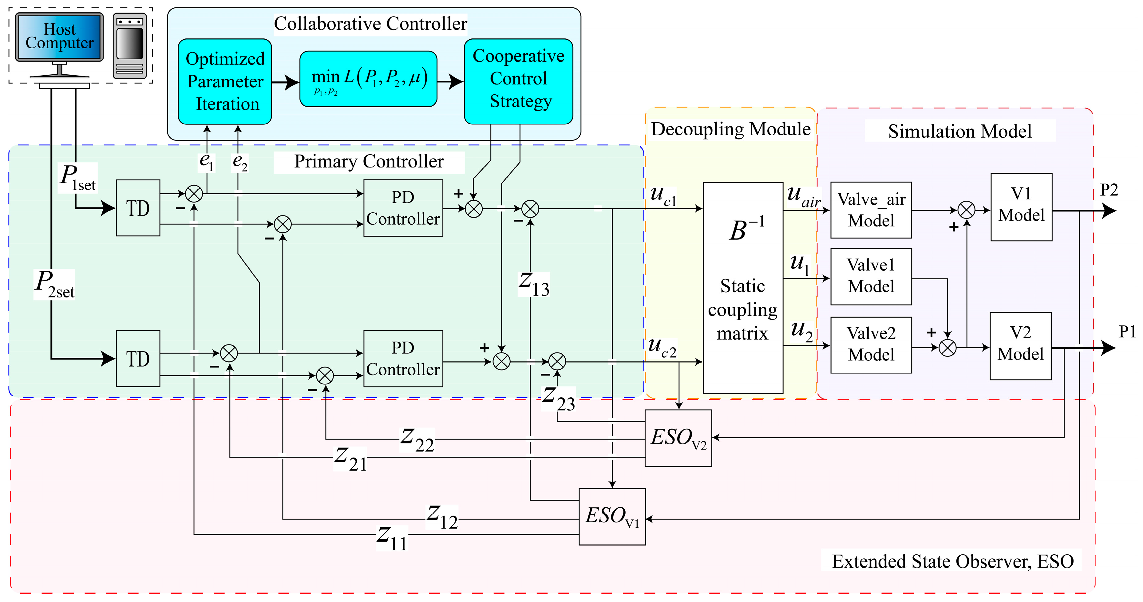
6.1. Simulation Verification Platform Setup

Based on the developed model and controller, a hardware-in-the-loop (HIL) simulation platform is built using a real-time simulator, a programmable logic controller (PLC), and MATLAB/Simulink (see Figure 6). The platform consists of three parts: the simulator, the PLC, and the host PC. The host PC provides a human–machine interface for entering control targets and system parameters. The simulation machine runs the complete intake system model, including the control-valve model, the chamber temperature–pressure differential model, and the boundary-condition model. The PLC implements the control algorithms, including the external penalty function optimization and the ADRC algorithm.

The real-time simulator operates on a Linux-based system and is equipped with two 3.3 GHz CPUs, each with 8 cores (16 threads), totaling 16 physical cores. It supports flexible core partitioning and is capable of executing large-scale, computation-intensive models with high real-time performance. In practice, the physical-model-based intake system is first constructed in MATLAB/Simulink. The resulting model is then converted into C code and deployed to the real-time simulator for execution within the HIL platform.

In the simulation, Gaussian noise was added to the two chamber output signals to emulate sensor disturbances in a real test environment: the temperature signal received noise in the range (−0.1, 0.1), and the pressure signal noise in the range (−2, 2). At the same time, the nonlinear function shown in Figure 4 was implemented as a 0.15 s delay element.

These simulations verify the intake-pressure control system’s tracking performance under the proposed controllers and its disturbance-rejection capability during abrupt flow changes.

6.2. Simulation Testing and Validation

To evaluate the performance of the proposed coordinated external-penalty ADRC method, a joint simulation of the intake system with two chambers and multiple valves was carried out. The inlet pressure and temperature of supply chamber V1 were set to 150 kPa and 253 K, respectively; the outlet pressure and temperature at V1’s exhaust control valve were set to 101.325 kPa and 288 K. The equivalent volumes of chambers V1 and V2 were specified as 300 m³ and 800 m³, respectively. The time constants of valves Valve1, Valve2, and Valve_air were set to 2.5 s, 1.5 s, and 2.5 s, with diameters of 2.6 m, 1.2 m, and 2.6 m, respectively.

Based on experimental requirements, desired pressure profiles and engine extraction flow rates were defined (see Figure 7) to assess control performance under various operating conditions. The control system composed of three independent PID loops served as the baseline. Comparative test results for the two control frameworks are shown in Figure 8. The control system parameters of the cooperative ADRC are listed in

Table 1. Main parameters of the cooperative ADRC.

Parameter	Value	Parameter	Value
$\gamma$	0.5	$\mu$	0.001
$\sigma$	0.01	$l$	0.2
${\omega }_1$	2	${\omega }_2$	5
$k_{11}$	0.001	$k_{12}$	0.0001
$k_{13}$	0.1	$k_{21}$	0.03
$k_{22}$	0.03	$k_{23}$	1

.

The penalty factor in the table is denoted by $\gamma$. Its value was chosen as 0.5 to reflect the relevant orders of magnitude. The parameters $\mu$ and $\sigma$ tune the penalty strength; since chamber V2’s pressure control is given higher priority, $\sigma$ carries the larger weight. The learning rate l was set to 0.2.

The bandwidths of the ADRCs for chambers V1 and V2 are denoted by ${\omega }_1$ and ${\omega }_2$, respectively. Based on the dynamic characteristics of each subsystem, they are set to ${\omega }_1=2,{\omega }_2=5$. Applying the bandwidth-based tuning method, the resulting ESO feedback gains for the two chambers are

$$\begin{array}{l}{\beta }_{11}=6,{{\beta }_{21}}^2=12,{\beta }_{13}=8\\ {\beta }_{21}=15,{\beta }_{22}=75,{\beta }_{23}=125\end{array}$$

For chamber V1, the control gains are $\left\{k_{11},k_{12},k_{13}\right\}$, and for chamber V2 they are $\left\{k_{21},k_{22},k_{23}\right\}$. In each set, the first two entries represent the proportional (K_p) and derivative (K_d) gains, while the third term is the coordination gain. The coordination gain in each chamber is chosen in proportion to the disturbance magnitude acting on that chamber.

Table 2. Parameters of the three-loop PID controller.

	KP	KI	KD
Valve 1	0.005	0.005	0.002
Valve 2	0.005	0.005	0.002
Valve_air	0.003	0.003	0.001

lists the parameters of the three-loop PID controller used as the baseline for comparison. The PID parameters were selected based on historical engineering practice. Specifically, as the system had previously used PID controllers in real applications, the PID controller parameters were initially set based on actual values used in prior deployments and then fine-tuned through simulation to improve convergence speed and steady-state accuracy.

To thoroughly evaluate the performance of the proposed control algorithm under various operating conditions of the high-flow intake system, three test phases were simulated:

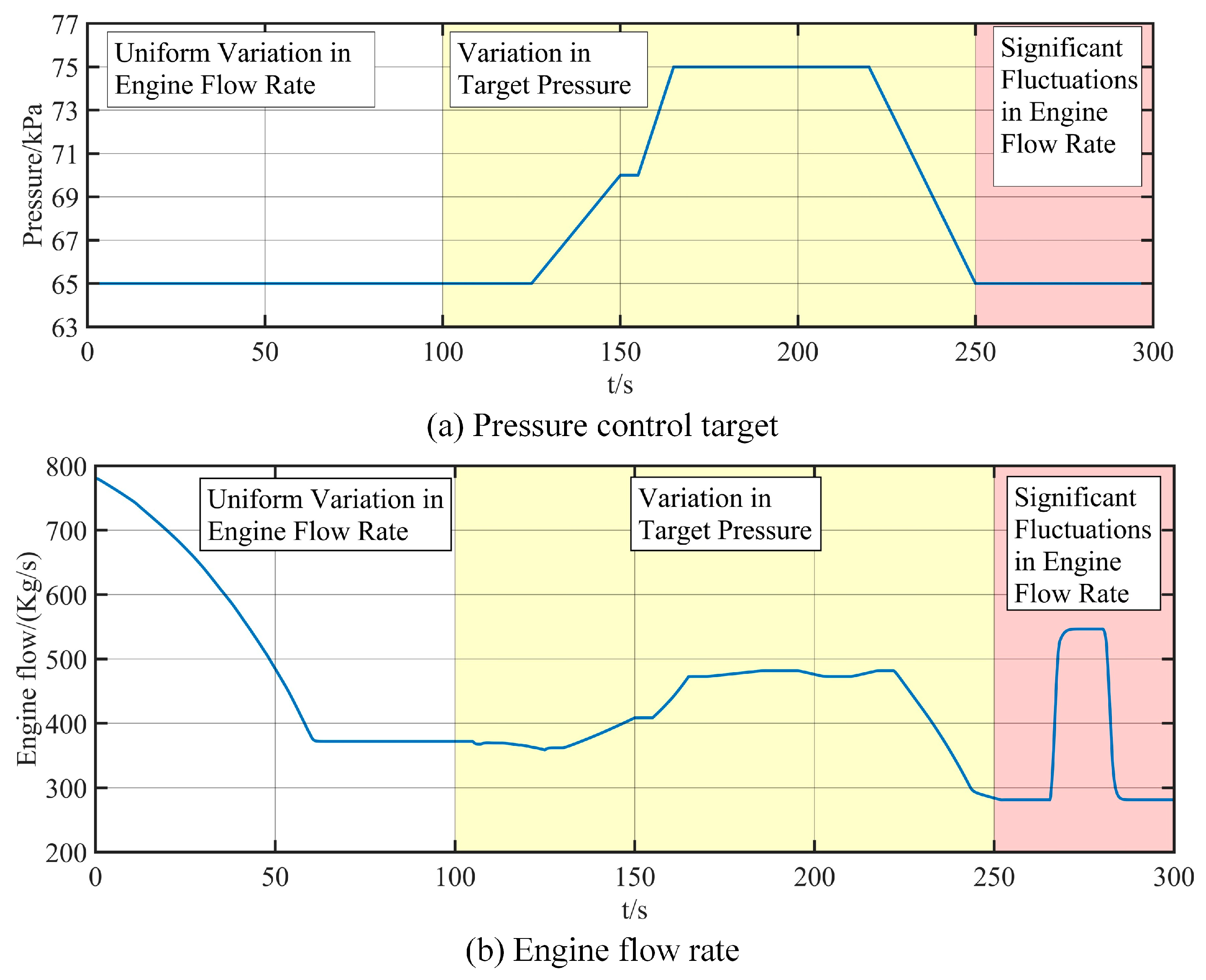
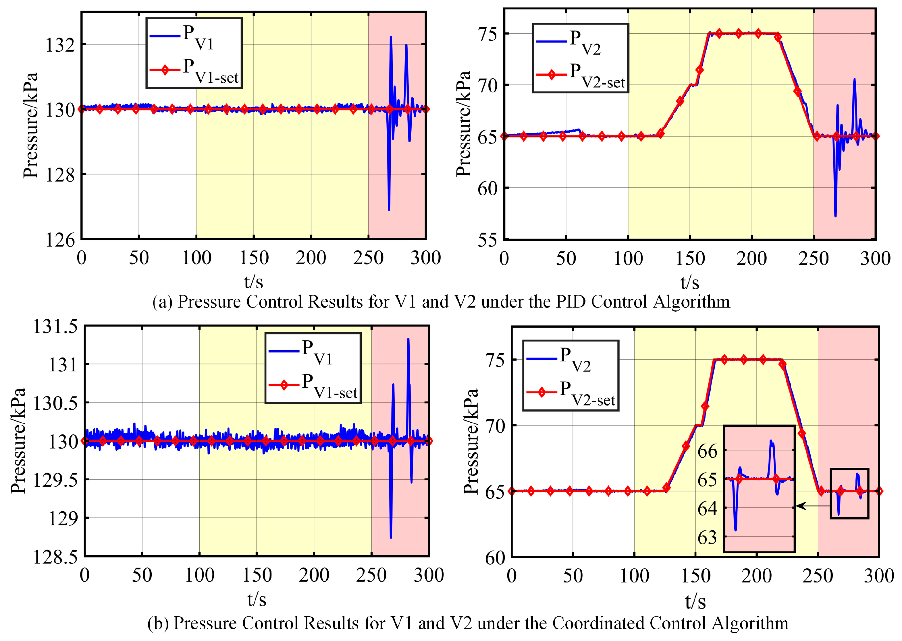
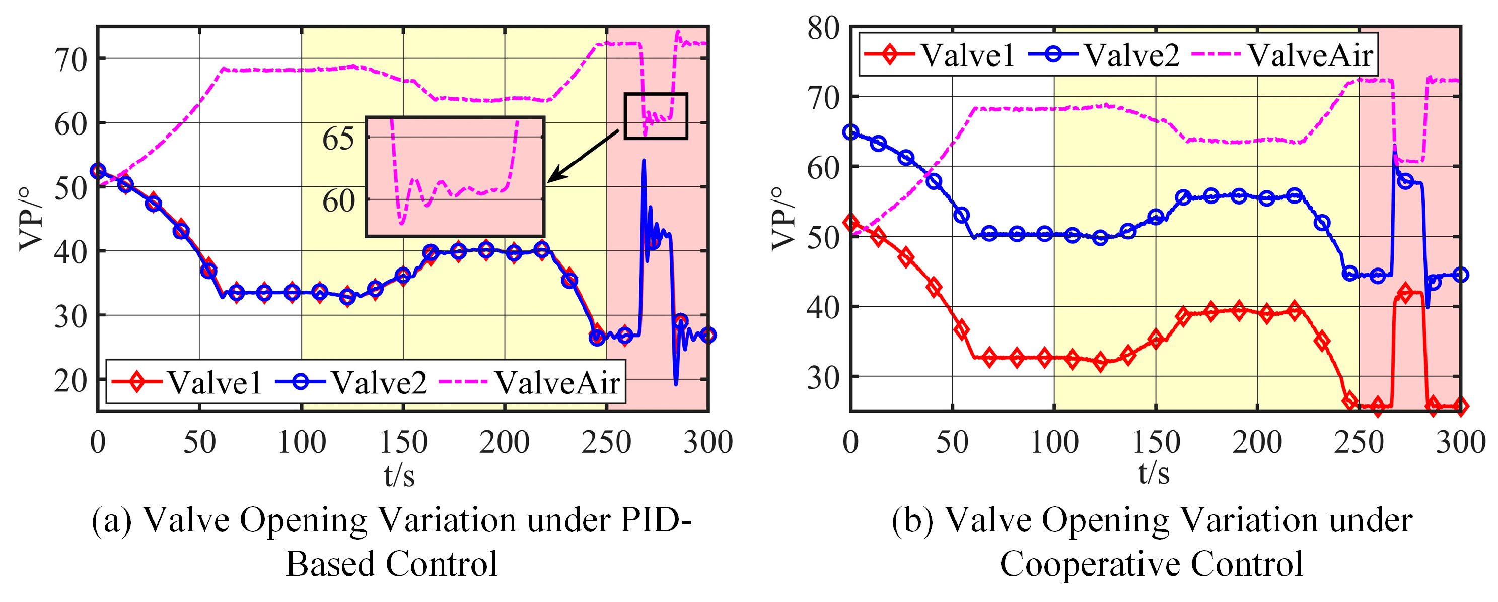
• 0–100 s (Uniform Flow Variation): Engine flow decreases smoothly from 780 kg/s to 370 kg/s over the first 60 s, then remains constant until 100 s. During this phase, V2’s setpoint is maintained at 65 kPa. This phase is designed to evaluate the pressure-holding capability of the control system under a prolonged and wide-range variation in engine flow.
• 100–250 s (Pressure Tracking): V2’s setpoint ramps from 65 kPa to 70 kPa at 125–150 s, holds until 155 s, then ramps to 75 kPa at 155–165 s and holds until 220 s; finally, it returns to 65 kPa at 220–250 s. Engine flow varies according to the engine mode [27]. This phase aims to assess the tracking performance of the controller in following dynamic pressure setpoints within a high-flow intake chamber.
• 250–300 s (Disturbance Rejection): Engine flow jumps from 280 kg/s to 550 kg/s over 265–270 s, then back to 280 kg/s over 280–285 s, with a peak rate of change of 80 kg/s². V2’s setpoint remains at 65 kPa. This phase is intended to test the disturbance rejection capability of the control system under abrupt and large-scale fluctuations in engine flow.

Throughout all tests, V1’s pressure setpoint was fixed at 130 kPa. As shown in Figure 8, the coordinated external-penalty ADRC delivers markedly better control quality than three independent PID loops, especially in the 250–300 s disturbance phase. The pressure error curves under both control schemes appear in Figure 9. A quantitative evaluation using the root mean square error (RMSE), the integral of absolute error (IAE), and the maximum absolute error (MaxAE) is summarized in

Table 3. Control performance index.

	RSME V1	RSME V2	IAE V1	IAE V2	MaxAE V1	MaxAE V2
Coordinated ADRC	0.123 kPa	0.218 kPa	18.051 kPa·s	33.175 kPa·s	1.327 kpa	1.782 kPa
PID	0.278 kPa	0.736 kPa	27.259 kPa·s	83.159 kPa·s	3.107 kPa	7.793 kPa

. The RMSE is defined as

$$\mathrm{RMSE}=\sqrt{{\displaystyle \frac{1}{N}}{\displaystyle \sum _{k=1}^N{e}^2}(k)}.$$

(38)

where N is the total number of signal points and e denotes the control error. The IAE accumulates the magnitude of the deviation:

$$\mathrm{IAE}={\displaystyle \sum _{k=1}^N|}e(k)|\Delta t.$$

(39)

MaxAE captures the worst instantaneous deviation:

$$\mathrm{Max}\mathrm{AE}={\max }_{1\le k\le N}|e(k)|.$$

(40)

Table 3 shows that three independent PID loops cannot keep both chamber pressures within the ± 3 kPa specification: chamber V2 reaches a peak error of 7.793 kPa and chamber V1 exceeds 3 kPa twice during 250–300 s. By contrast, the proposed coordinated ADRC always satisfies the constraint, limiting the maximum absolute error to 1.782 kPa (V2) and 1.327 kPa (V1).

A quantitative survey of the three performance indices confirms the visual impression:

• Average accuracy. Compared with PID, the ADRC reduces RMSE by 56% in V1 (0.278 → 0.123 kPa) and by 70% in V2 (0.736 to 0.218 kPa).
• Cumulative deviation. The integral of absolute error (IAE) falls from 27.259 to 18.051 $\mathrm{kPa}\cdot \mathrm{s}$ (−33%) in V1 and from 83.159 to 33.175 $\mathrm{kPa}\cdot \mathrm{s}$ (−60%) in V2, indicating that the coordinated strategy spends far less time operating with large errors.
• Worst-case behavior. MaxAE is reduced by a factor of 2.3 in V1 and 4.3 in V2, further demonstrating the superior robustness of the proposed coordinated ADRC under severe disturbances.

The valve-angle trajectories presented in Figure 10 elucidate the underlying control actions that lead to these performance differences. When the 250–300 s disturbance is applied, the PID system drives all three valves into large, mutually interfering oscillations (peak-to-peak ≈ 27% of full stroke); this cross-coupling propagates directly to the pressure channels and prolongs recovery. With the coordinated ADRC, the valves respond in a synchronized, non-oscillatory manner (peak-to-peak < 5%), and the chambers reach a steady state roughly 50% sooner, effectively decoupling the pressure dynamics of V1 and V2.

In summary, across the three representative operating phases—uniform flow variation (0–100 s), pressure-setpoint tracking (100–250 s), and transient disturbance rejection (250–300 s)—the external-penalty-function-based coordinated ADRC outperforms the three-loop PID benchmark in all three performance indices while continuously meeting the ±3 kPa specification. These results demonstrate that the proposed controller exhibits markedly superior robustness and convergence performance for multi-valve, multi-chamber pressure regulation in high-flow intake systems.

7. Conclusions

This paper addressed the challenges of multi-valve decoupling and strong-disturbance rejection in a high-altitude, multi-chamber intake system during engine transient tests. We proposed a coordinated ADRC method based on an external penalty function and validated it through theoretical analysis and hardware-in-the-loop (HIL) simulation. The main conclusions are as follows:

(1)

Pressure-Error Constraint via External Penalty

The chamber’s pressure safety limit was reformulated as an inequality-constrained optimization problem. An exponential penalty function, together with a gradient-based optimization algorithm, enables the dynamic relaxation of constraints and provides a feasible domain for multi-objective coordination. The algorithm’s global convergence was rigorously proven.

(2)

Multi-Valve Coordinated ADRC

We enhanced the existing distributed ADRC framework by integrating a coordination-optimization term with the disturbance-compensation mechanism. This yielded a multi-valve coordinated ADRC controller that overcomes the valve-saturation and pressure oscillation issues of traditional methods. Lyapunov stability theory guarantees the asymptotic stability of the closed-loop system.

(3)

HIL Simulation Results

Tests on a real-time simulator + PLC HIL platform show that the proposed method confines the V2 chamber’s pressure error within 3 kPa (maximum 1.782 kPa), a 77.1% reduction compared to PID control. Under a flow disturbance rate of 180 kg/s², valve-opening oscillations shrink by 81.5% (±5% vs. ±27%), confirming the method’s disturbance-rejection and decoupling capabilities.

This study has focused on pressure coordination in a dual-chamber intake system. Future work will introduce temperature parameters to develop a coupled pressure–temperature control model and investigate coordinated temperature–pressure control under high and low temperature transient conditions. This will enhance environmental simulation accuracy and overall stability in complex thermo-coupled systems.

References

1. Zhou, Q.; Guo, Y.; Zhao, W.; Xu, K.; Wang, K.; Wu, Z.; Sun, H. Research on fault diagnosis technology of simulated altitude test facility based on multi-optimization strategy, real-time data transfer, and the MH attention-RF algorithm. Multimed. Tools Appl. 2024, 83, 28729–28760. [Google Scholar] [CrossRef]
2. Zhu, M.; Wang, X. An integral type μ synthesis method for temperature and pressure control of flight environment simulation volume. In Turbo Expo: Power for Land, Sea, and Air; American Society of Mechanical Engineers: New York, NY, USA, 2017; V006T05A006. [Google Scholar]
3. Davis, M.; Montgomery, P. A flight simulation vision for aeropropulsion altitude ground test facilities. J. Eng. Gas Turbines Power 2005, 127, 8–17. [Google Scholar] [CrossRef]
4. Li, C.; Zhang, H.; Xiao, G.; Zhai, C.; Dan, Z.; Wang, X. An efficient tracking differentiator based active disturbance rejection control for flight environment simulation system. Aerosp. Sci. Technol. 2024, 155, 109578. [Google Scholar] [CrossRef]
5. Xu, Z.; Zhang, H.; Zhai, C.; Xiao, G.; Qian, Q.; Huang, F. Active Disturbance Rejection Intake Pressure Control of Aeropropulsion Systems Test Facility with Adaptive Parameter b0. Aerosp. Sci. Technol. 2025, 163, 110289. [Google Scholar] [CrossRef]
6. Liu, J.; Wang, X.; Liu, X.; Zhu, M.; Pei, X.; Dan, Z. μ-Synthesis control with reference model for aeropropulsion system test facility under dynamic coupling and uncertainty. Chin. J. Aeronaut. 2023, 36, 246–261. [Google Scholar] [CrossRef]
7. Walker, S.; Tang, M.; Mamplata, C. TBCC propulsion for a Mach 6 hypersonic airplane. In Proceedings of the 16th AIAA/DLR/DGLR International Space Planes and Hypersonic Systems and Technologies Conference, Bremen, Germany, 19–22 October 2009; p. 7238. [Google Scholar]
8. Pei, X.; Wang, X.; Liu, J.; Zhu, M.; Dan, Z.; He, A.; Miao, K.; Zhang, L.; Xu, Z. A review of modeling, simulation, and control technologies of altitude ground test facilities for control application. Chin. J. Aeronaut. 2023, 36, 38–62. [Google Scholar] [CrossRef]
9. Liu, J.; He, A.; Pei, X.; Long, Y. Feedforward compensation-based L1 adaptive control for aeropropulsion system test facility and hardware-in-the-loop verification. Chin. J. Aeronaut. 2025, 38, 103386. [Google Scholar] [CrossRef]
10. Miao, K.; Wang, X.; Zhu, M.; Zhang, S.; Dan, Z.; Liu, J.; Yang, S.; Pei, X.; Wang, X.; Zhang, L. A multi-cavity iterative modeling method for the exhaust systems of altitude ground test facilities. Symmetry 2022, 14, 1399. [Google Scholar] [CrossRef]
11. Liu, J.S.; Wang, X.; Zhu, M.Y.; Yang, S.; Pei, X.; Miao, K.; Zhang, S.; Dan, Z. Precise pressure control of constant pressure chamber based on control allocation. J. Propuls. Technol. 2022, 43, 383–391. (In Chinese) [Google Scholar]
12. Liu, J.S.; Yang, S.B.; Wang, X.; Zhu, M.; Pei, X.; Dan, Z.; Miao, K.; Zhang, S. Open loop–closed loop compound control method for pressure stabilizing chamber based on double-valve control. J. Propuls. Technol. 2022, 43, 339–346. (In Chinese) [Google Scholar]
13. Gao, Y.; Xu, R.; Wang, Y.; Tian, D. Multi-actuator control with modal switching and different disturbance for scanning imaging motion compensation. IET Control Theory Appl. 2021, 15, 1931–1941. [Google Scholar] [CrossRef]
14. Hu, S.; Kang, H.; Tang, H.; Cui, Z.; Liu, Z.; Ouyang, P. Trajectory optimization algorithm for a 4-DoF redundant parallel robot based on 12-phase sine jerk motion profile. Actuators 2021, 10, 80. [Google Scholar] [CrossRef]
15. Jayswal, A.; Arana-Jiménez, M. Robust penalty function method for an uncertain multi-time control optimization problems. J. Math. Anal. Appl. 2022, 505, 125453. [Google Scholar] [CrossRef]
16. Zheng, L.; Liu, W.; Zhai, C. A dynamic lane-changing trajectory planning algorithm for intelligent connected vehicles based on modified driving risk field model. Actuators 2024, 13, 380. [Google Scholar] [CrossRef]
17. Xiong, S.; Liu, H.H.-T. Low-altitude fixed-wing robust and optimal control using a barrier penalty function method. J. Guid. Control. Dyn. 2023, 46, 2218–2223. [Google Scholar] [CrossRef]
18. Espinosa Barcenas, O.U.; Quijada Pioquinto, J.G.; Kurkina, E.; Lukyanov, O. Multidisciplinary analysis and optimization method for conceptually designing of electric flying-wing unmanned aerial vehicles. Drones 2022, 6, 307. [Google Scholar] [CrossRef]
19. Wu, C.; Fang, H.; Yang, Q.; Zeng, X.; Wei, Y.; Chen, J. Distributed cooperative control of redundant mobile manipulators with safety constraints. IEEE Trans. Cybern. 2021, 53, 1195–1207. [Google Scholar] [CrossRef]
20. Mirzaei, A.; Ramezani, A. Distributed model predictive control for nonlinear large-scale systems based on reduced-order cooperative optimisation. Int. J. Syst. Sci. 2021, 52, 2427–2445. [Google Scholar] [CrossRef]
21. Tang, Y.; Ren, Z.; Li, N. Zeroth-order feedback optimization for cooperative multi-agent systems. Automatica 2023, 148, 110741. [Google Scholar] [CrossRef]
22. Han, J. From PID to active disturbance rejection control. IEEE Trans. Ind. Electron. 2009, 56, 900–906. [Google Scholar] [CrossRef]
23. Bandyopadhyay, S.; Qin, Z.; Bauer, P. Decoupling control of multiactive bridge converters using linear active disturbance rejection. IEEE Trans. Ind. Electron. 2020, 68, 10688–10698. [Google Scholar] [CrossRef]
24. Gao, Z. On the centrality of disturbance rejection in automatic control. ISA Trans. 2014, 53, 850–857. [Google Scholar] [CrossRef] [PubMed]
25. Wei, Q.; Wu, Z.; Zhou, Y.; Ke, D.; Zhang, D. Active disturbance-rejection controller (ADRC)-based torque control for a pneumatic rotary actuator with positional interference. Actuators 2024, 13, 66. [Google Scholar] [CrossRef]
26. Zhang, L.; Zhang, H.; Zhai, C.; Wang, X.; Dan, Z. A new time optimal control based tracking differentiator with small phase lag. In Proceedings of the 2024 43rd Chinese Control Conference (CCC), Kunming, China, 28–31 July 2024; IEEE: Piscataway, NJ, USA, 2024; pp. 908–912. [Google Scholar]
27. Long, Y.; Yang, S.; Wang, X.; Jiang, Z.; Liu, J.; Zhao, W.; Zhu, M.; Chen, H.; Miao, K.; Zhang, Y. MoHydroLib: An HMU Library for Gas Turbine Control System with Modelica. Symmetry 2022, 14, 851. [Google Scholar] [CrossRef]
Figure 1. Schematic diagram of system structure.
Actuators 14 00334 g001
Figure 2. Chamber structure diagram.
Actuators 14 00334 g002
Figure 3. Diagram of control valve model.
Actuators 14 00334 g003
Figure 4. Schematic diagram of the valve dynamic characteristic model.
Actuators 14 00334 g004
Figure 5. Schematic diagram of the pressure coordination control system.
Actuators 14 00334 g005
Figure 6. Schematic diagram of the HIL simulation platform.
Actuators 14 00334 g006
Figure 7. Test condition configuration.
Actuators 14 00334 g007
Figure 8. Verification results.
Actuators 14 00334 g008
Figure 9. Pressure control errors.
Actuators 14 00334 g009
Figure 10. Valve position variations.
Actuators 14 00334 g010