Abstract
Tracking control of a quadrotor–slung load system is extremely challenging due to its under-actuation property, couple effects, and various uncertainties. This work proposes a composite backstepping control framework combining command filter control and a multivariable finite-time disturbance observer to ensure robust position and orientation control for aerial payload transportation with high precision. Firstly, the kinematic and dynamic model under perturbations is derived based on Newton’s second law. The thrust control force consists of two orthogonal parts, each dedicated to regulating the position and orientation of the slung load independently. Then, hierarchical backstepping control generates the two parts in the load-translation and the load-orientation subsystems. Command filters are introduced into nonlinear backstepping to smoothen the control signals and overcome the problem of explosion of complexity. Additionally, to counteract the adverse effect of perturbations emerging in the linear velocity and angular velocity loops, multivariable finite-time observers are developed to ensure the estimation errors converge within a finite time horizon. Finally, comparative numerical simulation results validate the efficacy of the developed quadrotor–slung load tracking controller. Simulation results show that the proposed controller achieves smaller position tracking and orientation errors compared to traditional methods, demonstrating robust disturbance rejection and high-precision control.
1. Introduction
Recently, unmanned aerial transport systems for object delivery have attracted growing research and commercial interest [1,2]. Unmanned aerial transportation has demonstrated significant advantages across various applications, including parcel delivery in urban environments [3,4], supply distribution in conflict or disaster-stricken areas [5], and tasks such as crop monitoring and pesticide dispersion in precision agriculture [6], among others. Quadrotors have been extensively employed in aerial logistics operations on account of their vertical takeoff/landing capabilities, exceptional maneuverability, and straightforward mechanical configuration [7,8]. To enhance the maneuverability of quadrotor systems and improve the flexibility of their connection with payloads, quadrotor–slung load configurations have been developed. Such systems have been applied in various tasks, including water sampling [9] and package delivery [10].
The assumption of an inextensible cable leads to the introduction of two additional degrees of freedom in the system. Nevertheless, in most cases, incorporating extra actuators for controlling the swing of the payload is infeasible. Hence, the quadrotor transportation system in 3D space with a cable-suspended payload has eight degrees of freedom and only four control inputs. This under-actuation property makes the controller design challenging [11,12]. Additionally, the external disturbances and system uncertainties occurring in quadrotor dynamics further increase the difficulties in controller design [13,14].
In existing research, control strategies for load transportation using quadrotors are typically divided into two main categories. The first focuses on trajectory tracking of the quadrotor while actively suppressing the oscillations of the suspended load. Notable approaches within this category include dynamic programming techniques [15], input-shaping methods [16], and energy-based nonlinear control frameworks, where a carefully constructed energy function simultaneously captures the swing dynamics of the load and the trajectory-tracking performance of the quadrotor. Nevertheless, the controller proposed in [15] relies on linearizing the system dynamics, limiting its performance to local regions. The method in [16] ensures swing-free operation only when following a pre-defined trajectory. The energy-based method [17] suppresses swing motion effectively but is a relatively slow process.
An alternative methodology prioritizes payload-trajectory regulation. Prior work in [18] established that cable-suspended quadrotor–load systems admit representation as differentially flat hybrid systems with payload coordinates as flat outputs. This insight enabled development of a geometric regulation framework, achieving quasi-global exponential stabilization of payload trajectory tracking. Nevertheless, the singular perturbation-based convergence proofs detailed in [19] reveal sensitivity limitations when addressing unmodeled disturbances. Furthermore, the adaptive geometric controller in [19] ensures merely asymptotic error vanishing rather than exponential stabilization.
The backstepping technique in [20,21] has been widely applied to stabilize nonlinear dynamic systems, and is especially suitable for the quadrotor controller design, where different flight modes can be built due to the recursive structure of its dynamics. The dynamics of the quadrotor–slung load system do not conform to a strict-feedback form, making it unsuitable for direct stabilization via conventional backstepping methods. To overcome this challenge, the studies in [22,23] proposed a novel backstepping-inspired control framework. In their approach, a virtual thrust force is constructed to regulate the load’s position, while the quadrotor’s attitude and the cable direction are subsequently controlled to steer the actual thrust force towards the desired virtual force, thereby achieving trajectory tracking. However, no consideration about perturbations are introduced: all of the model parameters are assumed to be accurately known.
Recently, several advanced control strategies have been proposed for quadrotor–slung load systems to address the challenges of under-actuation, coupled dynamics, and external disturbances. For instance, a robust cascade observer was developed in [24] to handle multiple time-varying delays and uncertainties. This method achieves robust disturbance estimation and compensation using a cascade structure, but its compensation performance is limited to asymptotic convergence. Similarly, the work in [25] introduced a robust IDA-PBC framework tailored for under-actuated systems with inertia matrices dependent on unactuated coordinates. While this approach ensures stability under dynamic coupling and model uncertainties, it heavily relies on precise system modeling and exhibits limited robustness to large disturbances. Additionally, a predictive control strategy was proposed in [26] to optimize trajectory tracking for aerial payload transportation. Despite its high tracking accuracy, the computational complexity of predictive control may hinder its real-time applicability.
In this work, the control problem for the cable-suspended transportation system is tackled by applying a nonlinear backstepping framework. In the outer loop, the load-position tracking is controlled by the thrust along the cable, where the backstepped target cable-direction command is derived. Then, the inner-loop controller produces the force perpendicular to the current cable direction to force the cable direction to track the desired command. However, the conventional backstepping framework assumes accurate model parameters and neglects external disturbances, limiting its robustness in practical scenarios. To overcome these issues, a composite recursive control approach is adopted, which integrates a disturbance observer to compensate for external disturbances and modeling uncertainties in real time, employs command filtering to prevent signal explosion and ensure smooth control, and explicitly addresses the nonlinear coupling between translational and rotational dynamics. These enhancements make the proposed method more robust and effective for the cable-suspended transportation system compared to traditional approaches. To account for modeling imperfections, we consider typical uncertainties such as wind disturbances, drag on the load, and unknown payload mass. These are treated as lumped disturbances and estimated using disturbance observers. A multivariable finite-time disturbance observer (DO) is employed to estimate the lumped disturbances, and the effect of perturbances is attenuated by the online cancellation in the corresponding loop. After obtaining the desired quadrotor’s thrust command and combining it with the preset yaw angle, the residual dynamics system (the attitude dynamics) is fully actuated [22].
The main contributions of this work are as follows:
- This work proposes a composite command filter backstepping framework to achieve accurate and robust position and orientation tracking for a quadrotor–slung load system subject to perturbations. Command filter control is introduced at the velocity loop of the load-translation and the load-orientation subsystems. Compared with the method in [22], our approach effectively mitigates position and orientation tracking errors, resolves the “complexity explosion” from repeated differentiations, and cuts down measurement noise impacts [18].
- The adverse effects from unknown force perturbations are attenuated via the multivariable finite-time DO technique, which enables the lumped perturbations to be rapidly estimated and their effects to be counteracted online. Compared with [22,23], the composite strategy enhances the robustness and tracking accuracy, with faster disturbance estimation convergence.
- Lyapunov-based stability analysis rigorously establishes the uniformly ultimately bounded convergence of tracking errors under the proposed composite controller. Numerical simulations show this method outperforms [22] in disturbance rejection and control robustness for quadrotor–slung load systems.
For clarity of subsequent developments, some notation is introduced. The operator denotes the skew-symmetric matrix satisfying for any . Given a unit vector , the projection operator projects a vector along the direction of , i.e., . In contrast, the operator projects onto the plane perpendicular to , which can be expressed as .
2. Preliminaries
2.1. Problem Establishment
In modeling the quadrotor–slung load system, the quadrotor is treated as a rigid body with six degrees of freedom, while the load is considered a point mass with two degrees of freedom. The load is connected to the quadrotor’s center of mass via a fixed-length, taut cable. The dynamics of the system are expressed in a fixed inertial frame I and a body frame B fixed to the quadrotor’s center of mass, as shown in Figure 1. Unless specified otherwise, all vector quantities are formulated within the inertial coordinate system I. The body frame B, fixed relative to I, is parameterized by an element of the group, , with specifying the translational coordinates and representing the orientation matrix.
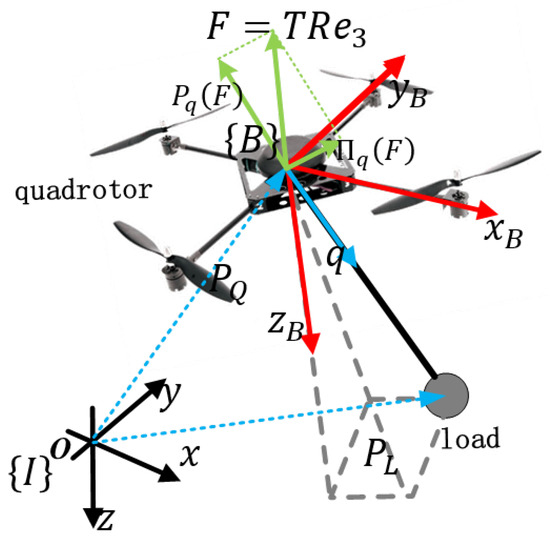
Figure 1.
Illustration of the quadrotor–slung load system.
Referring to the vector representation in Figure 1, we have
where represents the load’s position, l is the cable length, and is the unit vector indicating the cable’s direction. Here, is represented as a unit vector in for computation, with the constraint always maintained. Based on the circular motion shown in Figure 2, the kinematics of the load are described as follows:
where represents the angular velocity of the load in its circular motion, as expressed in the inertial frame I, and is always orthogonal to . Since is constrained to and the load follows a circular trajectory around the quadrotor’s center of mass, it follows that and .
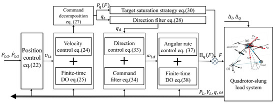
Figure 2.
Illustration of the proposed control framework.
Regarding the quadrotor’s geometric configuration, the four rotors generate thrust and torque vectors that are predominantly oriented perpendicular to their respective rotational planes. A high-bandwidth inner-loop controller is hypothesized to modulate torque for tracking reference angular velocity profiles, resulting in a quadrotor model accommodating omnidirectional angular velocity command inputs, whereas thrust vector alignment is preserved with the body-fixed vertical axis. By applying Newton’s second law to both the quadrotor and the load, the system dynamics are derived as
where and represent the velocities of the load and the quadrotor, respectively, while denotes the quadrotor’s mass; is the uncertain mass of the load, , where is the known nominal mass of the load; , is the thrust generated by the quadrotor’s motors; is the tension in the cable; g is the gravitational acceleration; denotes the unknown disturbing force for the quadrotor caused by gust and the system uncertainties; denotes the perturbing force for the slung load.
The second derivative of q is derived from (1) and (2), and their equivalence yields
By substituting from (3) and from (4), and then pre-multiplying both sides by , we obtain
Defining the thrust force of the quadrotor as , the full kinematic and dynamic model of the quadrotor–slung load system are expressed as
The disturbance term is
Equations (9), (10), and (11) are formulated by reorganizing and combining (7), (2), and (6), respectively. The quadrotor thrust force serves as the control input for the quadrotor–slung load system defined by (8)–(11). Consider a desired load trajectory , assumed to be at least of class with respect to time . The control objective is to design an appropriate control strategy for the quadrotor–slung load system governed by (8)–(11), where the actuation is realized through , with T and R denoting the thrust magnitude and the attitude of the quadrotor, respectively. The goal is to ensure that the load position accurately tracks the desired trajectory , such that the tracking error asymptotically converges to zero.
Assumption 1.
The quantities and are such that their first derivatives are bounded, i.e., and .
Assumption 2.
The desired trajectory is smooth and has bounded fourth-order derivatives (in space).
Assumption 3.
All system states—including position , linear velocity , cable direction , and angular velocity —are measurable or obtainable via onboard sensors (e.g., IMU, GPS, vision systems) and state estimation techniques.
Remark 1.
While and depend on system states (e.g., is a function of quadrotor velocity and wind velocity), the boundedness of and follows from two key aspects: (i) the physical constraints on disturbance rates (e.g., bounded wind acceleration), and (ii) that the closed-loop control ensures bounded state trajectories (Theorem 1), thereby limiting the rate of change of state-dependent disturbances.
Assumption 1, which addresses the boundedness of the first derivative, is a typical assumption in disturbance observer design [27,28]. The disturbances and are caused by parameter uncertainties, external perturbations, and unmodeled dynamics. Specifically, the parameter uncertainties arise from the system’s dependence on states (such as velocity, attitude angles, and angular rates) and certain unknown physical parameters. During normal flight operations, the system states are typically bounded to ensure the safe operation of the aerial system. Moreover, the external disturbances encountered in typical flight environments—provided there are no severe impacts—generally comply with these bounded conditions.
To guarantee smoothness and ensure system stability, the desired trajectory is required to be at least of class . Owing to the inherent under-actuation of the quadrotor–slung load system, the orientation of the load cannot be directly controlled or assigned arbitrarily. Instead, the evolution of the load’s direction naturally emerges from the control design procedure. Ultimately, the load’s motion and orientation are determined solely using the desired trajectory and its higher-order time derivatives; the differentially flat property of the system is leveraged.
Remark 2.
In our work, only the force for the quadrotor is generated to execute the control. Actually, the force command includes the thrust part (T) and the attitude part (). By assigning the yaw command (such as the yaw angle always remains at zero), the remaining system becomes fully actuated, which is a mature mode for the control system of a quadrotor [29,30].
2.2. Multivariable Finite-Time DO
The quadrotor–slung load system suffers from the effects of perturbations and uncertainties. The following multivariable finite-time DO is employed to estimate the lumped disturbance online, and attenuate the adverse effect of perturbations. Consider the system
where and denote the system state variables. The term represents an unknown but bounded disturbance, which is assumed to satisfy , with being a known positive constant that characterizes the upper bound of the perturbation. The coefficients and are control design parameters selected to ensure the desired system performance.
Lemma 1.
In order to stabilize the system (14), the control gains are required to meet the following conditions:
As a result, all trajectories asymptotically converge to the origin, i.e., , within a finite time. The convergence time is influenced by the parameters , , and the perturbation bound .
Consider the following perturbed system:
where represents the state vector, and is a known function of the state. The input to the system is denoted by , while represents the unknown disturbance vector, whose time derivative is bounded as , with being a constant. The matrix represents an invertible control gain. The finite-time disturbance observer is expressed as follows:
where and denote positive constant values.
Lemma 2.
Consider the system described in (17) subject to disturbances. By employing the observer defined in (18) with appropriately chosen parameters, the estimation error will asymptotically converge to zero within a finite time.
Proof.
Let the estimation error be defined as . The dynamics of the error are expressed as follows:
where represents the disturbance estimation error. Based on Lemma 1, it follows that the estimation error converges to zero in finite time. This leads to
□
Remark 3.
It is important to highlight that the multivariable finite-time disturbance observer (DO) is used to mitigate the impact of disturbances. While a scalar algorithm can be derived from the system’s decoupled structure (9), (11), employing the multivariable approach offers enhanced performance, including reduced chattering and broader applicability to certain non-decoupled uncertain systems [31,32].
Remark 4.
Disturbance observers have various implementations [33], and in this context, a finite-time DO [28,34] is employed to ensure the finite-time convergence of the estimation errors, which also contributes to the finite-time stability of the closed-loop system. The design parameters for the disturbance observers include , , , and . While larger values of these gains lead to faster convergence of the estimation errors, excessively large values may induce undesirable chattering effects. Therefore, the selection of these gains involves a trade-off.
3. Controller Design
According to the system dynamics in (8)–(11), it can be inferred that and can be manipulated independently via two orthogonal input components: and . In this structure, is responsible for steering toward the desired cable orientation, whereas modulates to govern the position of the payload. By employing a backstepping strategy for the translational motion of the load (subsystems (8) and (9)) and for the cable orientation dynamics (subsystems (10) and (11)), the control process begins with the construction of a virtual force , followed by the computation of , and eventually synthesizes the total control input applied to the quadrotor.
To achieve the defined control objectives, the control law is designed to minimize the trajectory-tracking error , ensuring that for all . Additionally, the disturbance observer is integrated into the control framework to guarantee finite-time disturbance rejection within . Closed-loop stability is ensured by designing the control inputs to satisfy the Lyapunov stability conditions. This backstepping-based scheme incorporates four cascaded control loops to generate the final control signal, as illustrated in Figure 2.
3.1. Loop 1: The Position of the Load
Define the tracking error of the load position . Following (8), its derivative is given as
The virtual velocity command is designed as
Thus, the dynamics of the position error can be rewritten as
3.2. Loop 2: The Velocity of the Load
Let the velocity error be . Following (9), we have
where . The target velocity command is designed as
where the nominal control part is applied to the nominal control performance for the system without perturbations. and are the designed control gains. is the estimation of the disturbance , which is given as
with the positive observer gains and , and under the conditions stated in Assumption 1 along with the result of Lemma 2, the disturbance estimation error is guaranteed to converge to zero in finite time, i.e.,
The desired direction of the cable is given as
Let the desired direction command vector pass through the low-pass filter to obtain the target command and its derivative as follows:
where the constant , measures angular deviation. Its magnitude (proportional to ) reflects the direction difference, with a negative sign.
Remark 5.
In the backstepping approach, a first-order command filter is employed to compute the time derivative of the desired command (), which is then used in the subsequent load-direction loop. This method, known as dynamic surface control [21,35] or command filter control [36], has become widely adopted in backstepping designs for high-order dynamic systems to prevent the “differential explosion” issue.
The control command is derived as
It is worth mentioning that expression (27) exhibits a singularity when approaches zero. Such a condition, however, is uncommon and generally arises during scenarios involving abrupt descent of the UAV. As highlighted in [37], this singularity issue can be alleviated by appropriately constraining the desired trajectory and tuning the control gains. Moreover, to robustly eliminate the potential singularity, a saturation strategy is incorporated as follows:
where denotes the third (vertical) component of the control vector , defined in (29). The vertical component of is restricted by a negative lower bound , which guarantees that the magnitude remains no less than a positive threshold . Substituting the virtual control into the error dynamics of the velocity tracking, yields
where and .
3.3. Loop 3: The Direction of the Load Cable
This loop aims to stabilize the direction of cable about the reference direction . Thus, the direction tracking error is defined as . Its derivative is
where . Continuing the backstepping procedure, the virtual angular rate command is given as
The low-pass filter for the virtual control command is given as
where is the positive filter gain. Substituting the virtual control design (33) into the error dynamics (32), yields
3.4. Loop 4: The Angular Velocity of the Cable
Define the tracking error of the angular rate of the load as . Following (11), this yields
Thus, the control input is designed as
with the positive control gain . is the estimation of the perturbation , which is given as
In light of Assumption 1 and Lemma 2, it can be inferred that the difference between the actual disturbance torque and its estimate will asymptotically vanish within a finite duration, i.e.,
Substituting the control design (37) into the error dynamics (36), yields
The final thrust command for the quadrotor is derived as
where .
3.5. The Proof of Stability
The closed-loop error dynamics can be divided into the inner-loop part (load-direction tracking) and the outer-loop part (position tracking), which are expressed as follows.
The inner-loop dynamics:
The outer-loop dynamics:
Before showing the main result of our controller, the following lemma is required to prove the stability of the closed-loop system.
Lemma 3.
According to [37], for bounded initial conditions, if a continuous and positive definite Lyapunov function exists that satisfies the inequality , where and are class functions, and if , with , being positive constants, then the solution is uniformly bounded.
The main conclusion of our proposed control system is summarized by the following theorem.
Theorem 1.
Under the dynamics of the quadrotor–slung load system described by (8)–(11), and considering the disturbance-related Assumptions 1 and 2, the designed composite backstepping controller augmented with a disturbance observer is defined in (41). This control strategy comprises the immediate control laws in (21), (24), and (33); the filtered target references in (28) and (34); as well as the disturbance estimation mechanisms given by (25) and (38). Under this framework, the complete closed-loop system exhibits uniform stability, and the tracking error of the load’s position converges to a bounded neighborhood asymptotically.
Proof.
Choose the positive Lyapunov candidate as follows:
where , , , and . The term with the max thrust value is employed to balance the effect for stability between the outer loop and inner loop. Following (43), the time derivative of is calculated as
According to (43), the derivative of is given as
Following the property of the direction vector and the analysis in Appendix A, gives that
Following the definition of , yields
where the constant is derived from the contraction of inequality. Thus, the time derivative satisfies that
Combining (42) and the relationship , the derivative of is given as
Following (42), we have
Combining the above analysis, it can be concluded that
Furthermore, the following representation is given:
where , , on . Following Lemma 3, to ensure closed-loop stability, the control gains should be chosen such that , i.e., , , , . One obtains that
There exist appropriately large control and observer gains such that the inequality holds. Based on the positive definiteness of V and the results from [38], the monotonic decrease in V, which is ensured by selecting sufficiently large control gains, implies that . Consequently, the solution in (54) holds for all .
Secondly, according to Lemma 2, the estimation errors are guaranteed to vanish within a finite time interval , i.e., and hold for all . Under this condition, the time derivative of the Lyapunov function V can be reduced to
where . By invoking Lemma 3, it follows that the Lyapunov candidate V remains bounded within an invariant set. Moreover, it yields
on . Considering the definition of V, the load-position tracking error is . By choosing sufficiently large control gains, the ultimate bound can be arbitrarily small.
Thus, the proof is completed. □
Remark 6.
For the proposed local-learning adaptive control framework, the proposed controller is composed of three parts: the nominal control component, the filter component, and the disturbance compensation component. The design of the nominal control gains , , , and is closely related to the dynamic characteristics of the physical system, which primarily governs the performance of the nominal system (excluding unknown disturbances), including aspects such as transient behavior, overshoot, and response speed. The parameters for disturbance elimination include and . Increasing these gains may accelerate the convergence, but results in chattering in the system response. Thus, there is a trade-off in deciding these parameters, usually depending on the results of the practical system performance.
4. Simulation
This section provides numerical simulation results to demonstrate the performance and efficacy of the proposed composite control strategy for the quadrotor–slung load system. The cable length is m. The mass of the quadrotor is set to kg, while the load mass is chosen as kg. Note that the mass of the load is uncertain, and its nominal value is taken as kg. To come close to the real situation, the force perturbation for the quadrotor and load are added into the simulation model.
The disturbance consists of the constant part and the time-varying part, which is given as
The uncertainty of the load system is mainly from the drag related to the wind speed, given as
Furthermore, the dynamics of the inner loop is simulated by the following first-order system:
where denotes the direction of the desired thrust direction of the quadrotor. The time constant of the filter system is selected as .
The proposed compound backstepping controller (named “Proposed”) is given in (41), with the parameters for each part as follows: , , , and for the standard tracking performance of the closed-loop system; and for the finite-time DO part; and for the command filter part.
To explicitly illustrate the necessity of considering the load dynamics and its induced disturbances on the quadrotor during controller design, a conventional quadrotor controller (denoted as “quad”) is implemented on the quadrotor–slung load system to track the reference trajectory , where represents the desired trajectory of the suspended load. Meanwhile, the adaptive backstepping control strategy is formulated as
with the control gain , , . The term is an integral adaptive term to attenuate the effect of perturbations.
To evaluate the effectiveness of the proposed composite recursive control strategy, we conducted a quantitative performance analysis using three key metrics: Root-mean-square error (RMSE) to quantify position tracking accuracy, settling time to measure the system response speed, and control effort to assess the peak thrust required for ensuring actuator hardware compatibility.
Furthermore, to exhibit the robustness of the proposed compound backstepping controller, the standard control system without the disturbance estimation (named “w/o DO”) is employed as a comparative case. Its framework and control gains are the same as the “proposed” except without the finite-time DO part. The simulation was conducted in the MATLAB environment on a laptop equipped with an i7-6700HQ CPU. The simulation sampling frequency was set to 100 Hz. This frequency defined the fixed time step (10 ms) at which the entire closed-loop system dynamics were numerically integrated, all controller components (including the four cascaded control loops, command filters, and disturbance observers) were executed, and all state measurements were sampled and feedback signals computed. The average computation time required by the proposed control algorithm over a 15 s simulation was 1.683 ms in MATLAB, reflecting a computational complexity of approximately . This complexity arises from 3 × 3 matrix-vector operations (e.g., , , Equations (21), (24) and (33)) and vector computations in the command filter (Equations (28), (34), and ) and disturbance observer (Equations (25), (38), and ), making it highly efficient. The computation time, well below the 10 ms sampling period, ensures suitability for real-time implementation on embedded platforms like STM32 or NVIDIA Jetson, consistent with similar controllers [22,25]. To evaluate the effectiveness of the controllers, two simulation scenarios were designed and carried out. Two simulated cases were used to test the performance of these controllers. To comprehensively analyze the performance, the following two cases were built to test these controllers.
4.1. Case 1: Hover at Fixed Point
The desired command is . The simulation results of the proposed controller are depicted in Figure 3 and Figure 4. The main performance comparison of the case is given in Table 1. It is demonstrated that the proposed control system is able to force the load to quickly reach, and accurately remain at, the target point. The “w/o DO” controller possess little robustness against perturbations, such that large position-tracking errors emerge. The finite-time disturbance observer (DO) integrated in the proposed control scheme exhibits superior capability in estimating and compensating for external disturbances. Consequently, the desired nominal tracking performance of the system can be effectively recovered. The “quad” controller cannot achieve precise hovering at a fixed point due to the swing of the load. It is concluded that feedback based on the direction of the cable is helpful to attenuate the effect of the load’s swing.
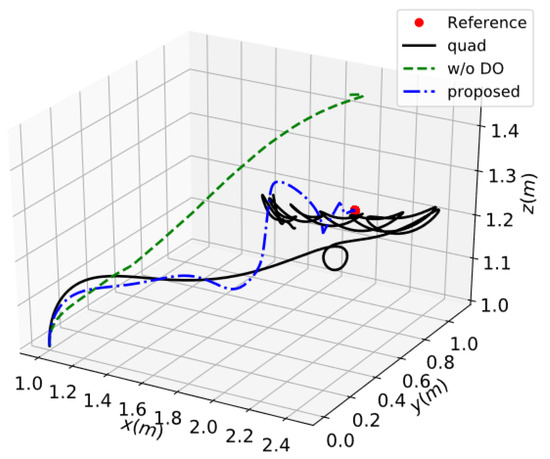
Figure 3.
The response of 3D position in case 1.
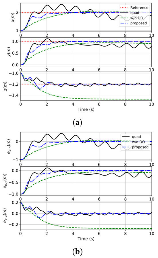
Figure 4.
The tracking error of the load’s position in case 1. (a) The response of the position of the load. (b) The tracking error of the load’s position.

Table 1.
Performance comparison of case 1.
Figure 5 shows the responses of the load-velocity tracking, which further illustrate this conclusion. The estimation result of the disturbances is given in Figure 6. The finite-time DO can estimate the disturbance online, and the estimation errors quickly converge to a small region of zeros. Figure 7 presents the control inputs of these methods. Violent oscillations in the control commands occur at the beginning due to the large initial error.
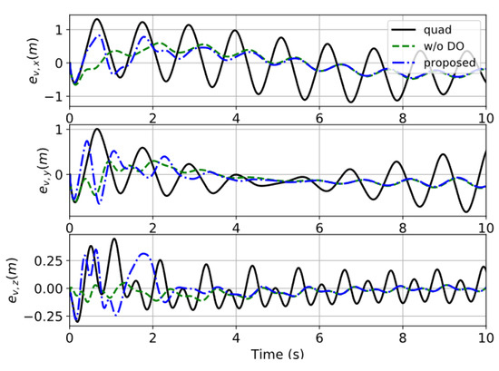
Figure 5.
The tracking error of the load’s velocity in case 1.
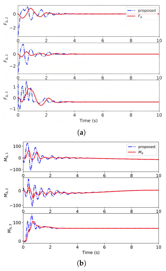
Figure 6.
The results of disturbance estimation in case 1. (a) The estimation of force disturbances. (b) The estimation of moment disturbances.
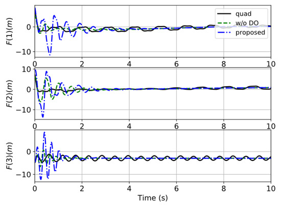
Figure 7.
The response of the control commands in case 1.
4.2. Case 2: Trajectory-Tracking Simulation
The desired circle-shape reference trajectory is described as follows:
The quadrotor–load system is commanded to track a circular trajectory while performing a lifting maneuver. This scenario enables a comprehensive evaluation of the system’s performance in terms of vertical ascent, lateral motion, and forward tracking capabilities.
The results are presented in Figure 8, Figure 9 and Figure 10. A performance comparison of the trajectory-tracking case is given in the following Table 2. Again, the proposed control framework for the quadrotor–slung load control problem can achieve high-performance position tracking of the load. Without the DOs, the controller fails to guarantee high-precision tracking performance for the desired trajectory.
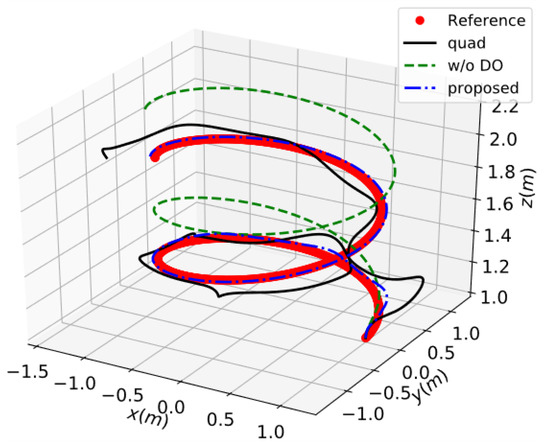
Figure 8.
The response of 3D position in case 2.
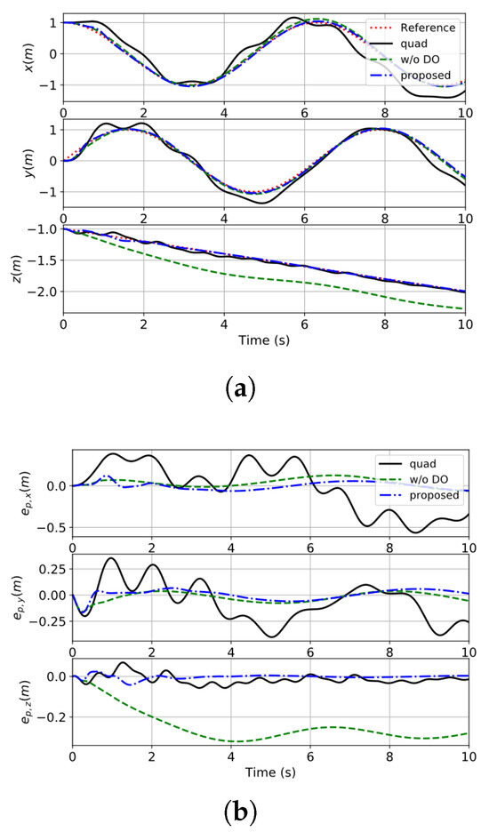
Figure 9.
The tracking error of the load’s position in case 2. (a) The response of the position of the load. (b) The tracking error of the load’s position.
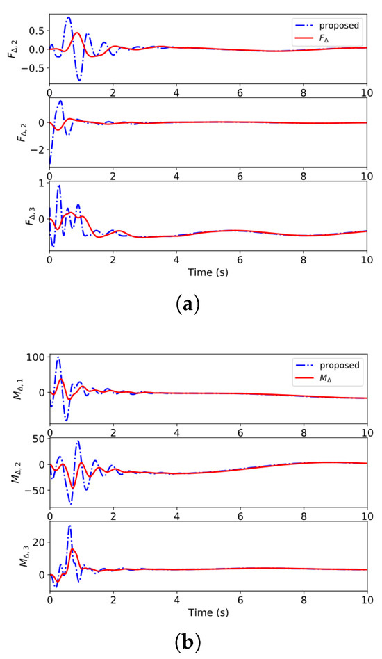
Figure 10.
The results of disturbance estimation in case 2. (a) The estimation of force disturbances. (b) The estimation of moment disturbances.
Table 2.
Performance comparison of case 2.
The swing is obvious in the “quad” control system due to the lack of load-state feedback. The results of disturbance estimation in case 2 are presented in Figure 10. In conclusion, the disturbance-observer-based composite backstepping control scheme for quadrotor–slung load system possesses superior tracking performance and robustness against perturbations and uncertainties.
4.3. Case 3: Trajectory Tracking with Measurement Noise
To assess the robustness of the proposed controller under more realistic operating conditions incorporating sensor imperfections, an additional simulation case was conducted. This case replicated the circular trajectory-tracking task defined in case 2. However, realistic measurement noise was introduced to the position and linear velocity states provided as feedback to the controller. Specifically, zero-mean Gaussian white noise was added with standard deviations of m for position and m/s for velocity, simulating typical noise levels encountered with onboard GPS and IMU sensors. All other simulation parameters and controller gains remained identical to case 2.
The results of case 3, incorporating realistic sensor noise, are presented in Figure 11 and Figure 12. Despite the introduction of significant measurement noise ( m for position and m/s for velocity), the proposed control framework maintains robust trajectory-tracking performance. These results confirm that the disturbance-observer-based composite backstepping control maintains its robustness against practical sensor imperfections typically encountered in real-world GPS and IMU systems, effectively compensating for measurement uncertainties while preserving tracking accuracy.
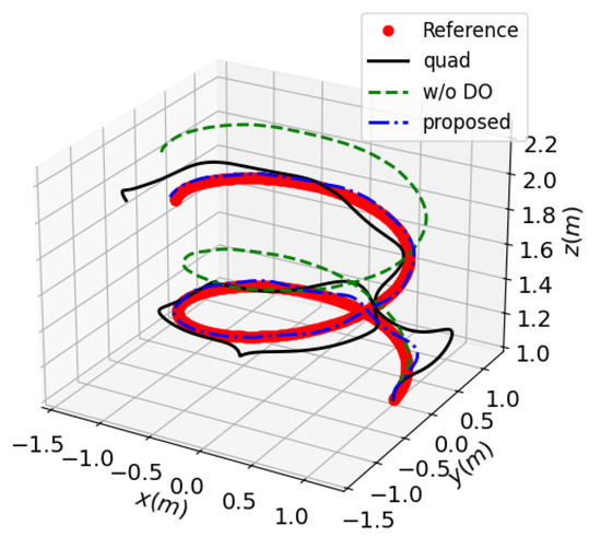
Figure 11.
The response of 3D position in case 3.
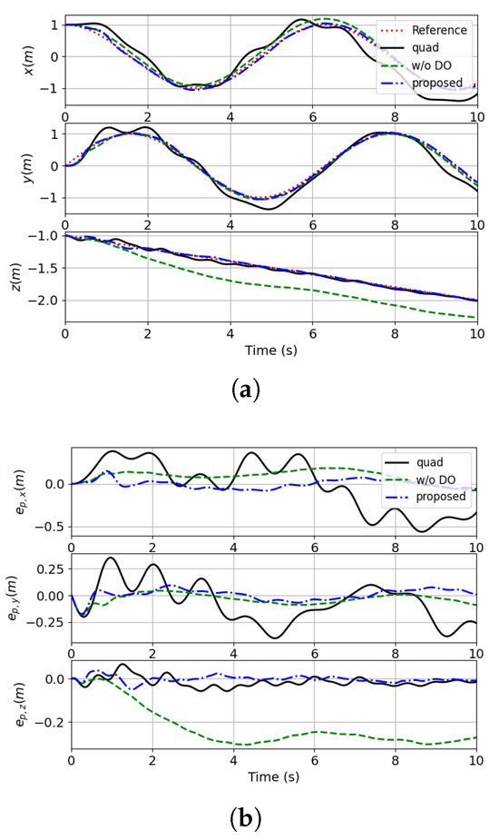
Figure 12.
The tracking error of the load’s position in case 3. (a) The response of the position of the load. (b) The tracking error of the load’s position.
5. Experiment
To validate the proposed control framework under practical conditions, flight tests were conducted using a custom-built quadrotor–slung load platform, as shown in Figure 13, and its experiment integration is shown in Figure 14. The quadrotor carried a 0.05 kg payload suspended by a 0.4 m cable. In addition, an array of motion capture cameras was used to identify the markers attached to the top of the load and the motion states of the load were obtained through an image processing computer.
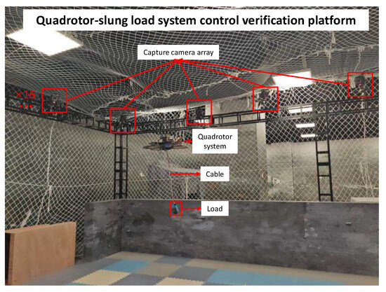
Figure 13.
The environment of the validation platform.
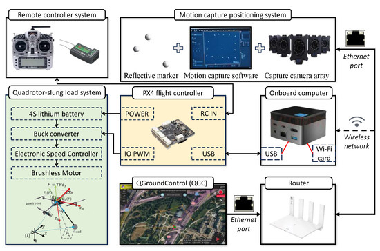
Figure 14.
Equipment integration of validation platform.
The desired circle-shape reference trajectory is described as follows:
The quadrotor–load system was commanded to track a circular trajectory while performing a lifting maneuver. The proposed compound backstepping controller is given in (41), with the parameters for each part as follows: , , , and for the standard tracking performance of the closed-loop system; and for the finite-time DO part; and for the command filter part.
The experimental results of the circular trajectory tracking are presented in Figure 15 and Figure 16. These results clearly demonstrate the practical applicability and robustness of the proposed control framework when deployed in real-world physical environments. Specifically, the controller maintains accurate trajectory-tracking performance under external disturbances and dynamic conditions, thereby validating its effectiveness beyond simulation scenarios.
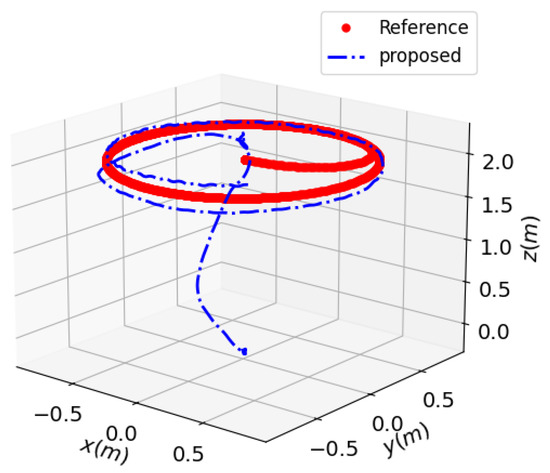
Figure 15.
Response of 3D position in real-world experiment.
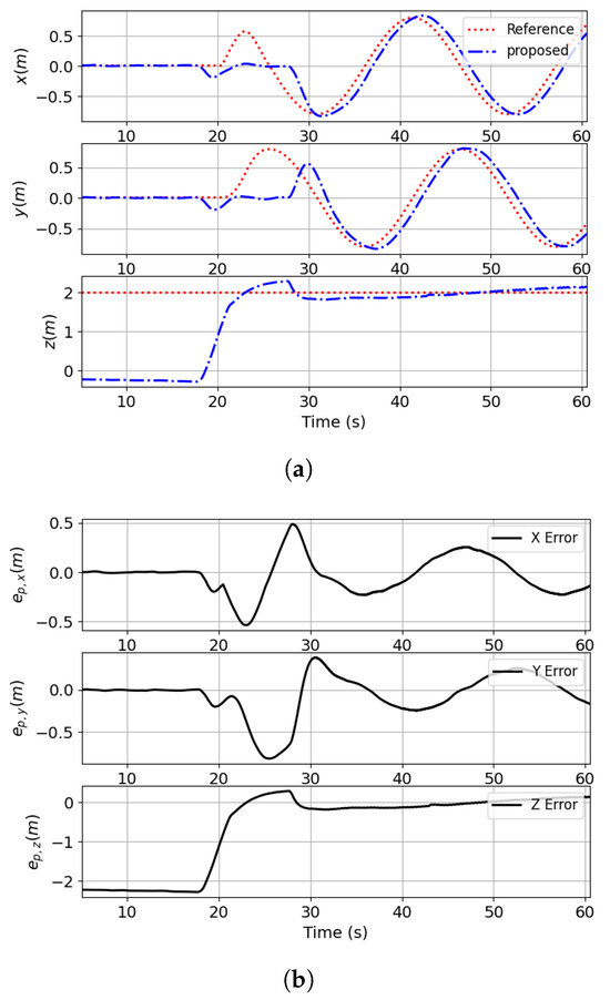
Figure 16.
The tracking error of the load’s position in real-world experiment. (a) The response of the position of the load. (b) The tracking error of the load’s position.
6. Conclusions
This work develops a composite recursive control methodology implemented for quadrotor-suspended payload systems operating under uncertainties, aiming to achieve precise trajectory tracking of the payload. A stepped control design constructs orthogonal virtual thrust vectors for simultaneous position regulation and attitude stabilization of the suspended load. To circumvent computational complexity escalation from virtual command differentiation, first-order command filters are integrated into both the velocity control loop and directional stabilization loop. Concurrently, a multivariable finite-time disturbance observer is synthesized to estimate and compensate aggregated uncertainties caused by external disturbances. Closed-loop stability is rigorously established via Lyapunov-based analysis, demonstrating uniformly ultimately bounded error convergence. Numerical simulations substantiate the trajectory-tracking performance and disturbance rejection capability of the proposed architecture. The method’s reliability is confirmed by robust disturbance rejection, with smaller errors compared with the traditional methods, supported by numerical simulations. The method’s advantages include high accuracy and real-time efficiency, while its limitations involve state constraints and actuator saturation. Furthermore, with a computational complexity of and an average computation time of 1.683 ms per cycle, the algorithm is well suited for real-time implementation on standard embedded hardware like STM32 or NVIDIA Jetson.
Although the proposed method has been validated through both simulation and real-world experiments, its performance under highly dynamic conditions and large-scale systems remains to be fully explored. Future work will focus on extending the approach to more complex flight scenarios and addressing practical issues such as state constraints and actuator saturation.
Author Contributions
Conceptualization, J.X. and J.Y.; methodology, J.X. and J.Y.; software, J.X.; validation, J.X. and D.L.; formal analysis, J.X. and D.L.; investigation, J.X. and D.L.; writing—original draft preparation, J.X. and D.L.; writing—review and editing, J.Y.; visualization, J.X. and D.L.; supervision, T.J.; project administration, T.J.; funding acquisition, J.Y. All authors have read and agreed to the published version of the manuscript.
Funding
This research received no external funding.
Data Availability Statement
Data are contained within the article.
Conflicts of Interest
The authors declare no conflicts of interest.
Appendix A. Calculation of
Following the property of the unit vector of direction yields
Further, one has
Combining the above representation, we have
Substituting (A3) into gives
References
- Zhang, X.; Huang, J.; Huang, Y.; Huang, K.; Yang, L.; Han, Y.; Wang, L.; Liu, H.; Luo, J.; Li, J. Intelligent amphibious ground-aerial vehicles: State of the art technology for future transportation. IEEE Trans. Intell. Veh. 2022, 8, 970–987. [Google Scholar] [CrossRef]
- Palunko, I.; Cruz, P.; Fierro, R. Agile load transportation: Safe and efficient load manipulation with aerial robots. IEEE Robot. Autom. Mag. 2012, 19, 69–79. [Google Scholar] [CrossRef]
- Kotaru, P.; Wu, G.; Sreenath, K. Differential-flatness and control of quadrotor(s) with a payload suspended through flexible cable(s). In Proceedings of the 2018 Indian Control Conference (ICC), Kanpur, India, 4–6 January 2018; IEEE: Piscataway, NJ, USA, 2018; pp. 352–357. [Google Scholar]
- Narazaki, Y.; Hoskere, V.; Chowdhary, G.; Spencer, B.F., Jr. Vision-based navigation planning for autonomous post-earthquake inspection of reinforced concrete railway viaducts using unmanned aerial vehicles. Autom. Constr. 2022, 137, 104214. [Google Scholar] [CrossRef]
- Tang, S.; Wüest, V.; Kumar, V. Aggressive flight with suspended payloads using vision-based control. IEEE Robot. Autom. Lett. 2018, 3, 1152–1159. [Google Scholar] [CrossRef]
- Guerrero, M.E.; Mercado, D.; Lozano, R.; García, C. Passivity based control for a quadrotor UAV transporting a cable-suspended payload with minimum swing. In Proceedings of the 2015 54th IEEE Conference on Decision and Control (CDC), Osaka, Japan, 15–18 December 2015; IEEE: Piscataway, NJ, USA, 2015; pp. 6718–6723. [Google Scholar]
- Liang, X.; Zhang, Z.; Yu, H.; Wang, Y.; Fang, Y.; Han, J. Antiswing Control for Aerial Transportation of the Suspended Cargo by Dual Quadrotor UAVs. IEEE/ASME Trans. Mechatron. 2022, 27, 5159–5172. [Google Scholar] [CrossRef]
- Yu, H.; Liang, X.; Han, J.; Fang, Y. Adaptive Trajectory Tracking Control for the Quadrotor Aerial Transportation System Landing a Payload Onto the Mobile Platform. IEEE Trans. Ind. Inform. 2024, 20, 23–37. [Google Scholar] [CrossRef]
- Ore, J.P.; Detweiler, C. Sensing water properties at precise depths from the air. J. Field Robot. 2018, 35, 1205–1221. [Google Scholar] [CrossRef]
- Guerrero-Sánchez, M.E.; Mercado-Ravell, D.A.; Lozano, R.; García-Beltrán, C.D. Swing-attenuation for a quadrotor transporting a cable-suspended payload. ISA Trans. 2017, 68, 433–449. [Google Scholar] [CrossRef]
- Chen, T.; Shan, J. Distributed tracking of a class of underactuated Lagrangian systems with uncertain parameters and actuator faults. IEEE Trans. Ind. Electron. 2019, 67, 4244–4253. [Google Scholar] [CrossRef]
- Chen, L.; Liu, Z.; Dang, Q.; Zhao, W.; Wang, G. Robust trajectory tracking control for a quadrotor using recursive sliding mode control and nonlinear extended state observer. Aerosp. Sci. Technol. 2022, 128, 107749. [Google Scholar] [CrossRef]
- Li, B.; Zhu, X. A novel anti-disturbance control of quadrotor UAV considering wind and suspended payload. In Proceedings of the 2023 6th International Symposium on Autonomous Systems (ISAS), Nanjing, China, 23–25 June 2023; pp. 1–6. [Google Scholar] [CrossRef]
- Ullah, H.; Zarin, O.; Ahmad, I.; Ahmad, S.; Abbas, A.; Lippiello, V. Robust Sliding Mode Control of a Quadrotor with Disturbance Rejection for Enhanced Stability and Performance. In Proceedings of the 2024 International Conference on Robotics and Automation in Industry (ICRAI), Rawalpindi, Pakistan, 18–19 December 2024; pp. 1–7. [Google Scholar] [CrossRef]
- Palunko, I.; Fierro, R.; Cruz, P. Trajectory generation for swing-free maneuvers of a quadrotor with suspended payload: A dynamic programming approach. In Proceedings of the 2012 IEEE International Conference on Robotics and Automation, Saint Paul, MN, USA, 14–18 May 2012; IEEE: Piscataway, NJ, USA, 2012; pp. 2691–2697. [Google Scholar]
- Klausen, K.; Fossen, T.I.; Johansen, T.A. Nonlinear control of a multirotor UAV with suspended load. In Proceedings of the 2015 International Conference on Unmanned Aircraft Systems (ICUAS), Denver, CO, USA, 9–12 June 2015; IEEE: Piscataway, NJ, USA, 2015; pp. 176–184. [Google Scholar]
- Xian, B.; Wang, S.; Yang, S. Nonlinear adaptive control for an unmanned aerial payload transportation system: Theory and experimental validation. Nonlinear Dyn. 2019, 98, 1745–1760. [Google Scholar] [CrossRef]
- Sreenath, K.; Lee, T.; Kumar, V. Geometric control and differential flatness of a quadrotor UAV with a cable-suspended load. In Proceedings of the 52nd IEEE Conference on Decision and Control, Firenze, Italy, 10–13 December 2013; IEEE: Piscataway, NJ, USA, 2013; pp. 2269–2274. [Google Scholar]
- Lee, T. Geometric control of quadrotor UAVs transporting a cable-suspended rigid body. IEEE Trans. Control Syst. Technol. 2017, 26, 255–264. [Google Scholar] [CrossRef]
- Wang, D.; Huang, J. Neural network-based adaptive dynamic surface control for a class of uncertain nonlinear systems in strict-feedback form. IEEE Trans. Neural Netw. 2005, 16, 195–202. [Google Scholar] [CrossRef] [PubMed]
- Pan, Y.; Yu, H. Composite learning from adaptive dynamic surface control. IEEE Trans. Autom. Control 2015, 61, 2603–2609. [Google Scholar] [CrossRef]
- Yu, G.; Cabecinhas, D.; Cunha, R.; Silvestre, C. Nonlinear backstepping control of a quadrotor-slung load system. IEEE/ASME Trans. Mechatron. 2019, 24, 2304–2315. [Google Scholar] [CrossRef]
- Cabecinhas, D.; Cunha, R.; Silvestre, C. A trajectory tracking control law for a quadrotor with slung load. Automatica 2019, 106, 384–389. [Google Scholar] [CrossRef]
- Hernández-González, O.; Targui, B.; Valencia-Palomo, G.; Guerrero-Sánchez, M. Robust cascade observer for a disturbance unmanned aerial vehicle carrying a load under multiple time-varying delays and uncertainties. Int. J. Syst. Sci. 2024, 55, 1056–1072. [Google Scholar] [CrossRef]
- Guerrero-Sánchez, M.E.; Hernández-González, O.; Valencia-Palomo, G.; Mercado-Ravell, D.A.; López-Estrada, F.R.; Hoyo-Montaño, J.A. Robust IDA-PBC for under-actuated systems with inertia matrix dependent of the unactuated coordinates: Application to a UAV carrying a load. Nonlinear Dyn. 2021, 105, 3225–3238. [Google Scholar] [CrossRef]
- Urbina-Brito, N.; Guerrero-Sánchez, M.E.; Valencia-Palomo, G.; Hernández-González, O.; López-Estrada, F.R.; Hoyo-Montaño, J.A. A Predictive Control Strategy for Aerial Payload Transportation with an Unmanned Aerial Vehicle. Mathematics 2021, 9, 1822. [Google Scholar] [CrossRef]
- Li, S.; Yang, J.; Chen, W.H.; Chen, X. Disturbance Observer-Based Control: Methods and Applications; CRC Press: Boca Raton, FL, USA, 2014. [Google Scholar]
- Jiang, T.; Lin, D.; Song, T. Finite-time control for small-scale unmanned helicopter with disturbances. Nonlinear Dyn. 2019, 96, 1747–1763. [Google Scholar] [CrossRef]
- Mahony, R.; Kumar, V.; Corke, P. Multirotor aerial vehicles: Modeling, estimation, and control of quadrotor. IEEE Robot. Autom. Mag. 2012, 19, 20–32. [Google Scholar] [CrossRef]
- Jiang, T.; Huang, J.; Li, B. Composite adaptive finite-time control for quadrotors via prescribed performance. J. Frankl. Inst. 2020, 357, 5878–5901. [Google Scholar] [CrossRef]
- Nagesh, I.; Edwards, C. A multivariable super-twisting sliding mode approach. Automatica 2014, 50, 984–988. [Google Scholar] [CrossRef]
- Jiang, T.; Lin, D. Fast finite-time backstepping for helicopters under input constraints and perturbations. Int. J. Syst. Sci. 2020, 51, 2868–2882. [Google Scholar] [CrossRef]
- Chen, W.H.; Yang, J.; Guo, L.; Li, S. Disturbance-observer-based control and related methods—An overview. IEEE Trans. Ind. Electron. 2015, 63, 1083–1095. [Google Scholar] [CrossRef]
- Wang, N.; Karimi, H.R.; Li, H.; Su, S.F. Accurate trajectory tracking of disturbed surface vehicles: A finite-time control approach. IEEE/ASME Trans. Mechatron. 2019, 24, 1064–1074. [Google Scholar] [CrossRef]
- Butt, W.A.; Yan, L.; Amezquita, S.K. Adaptive integral dynamic surface control of a hypersonic flight vehicle. Int. J. Syst. Sci. 2015, 46, 1717–1728. [Google Scholar] [CrossRef]
- Phan, V.D.; Truong, H.V.A.; Ahn, K.K. Actuator failure compensation-based command filtered control of electro-hydraulic system with position constraint. ISA Trans. 2023, 134, 561–572. [Google Scholar] [CrossRef]
- Antonelli, G.; Cataldi, E.; Arrichiello, F.; Giordano, P.R.; Chiaverini, S.; Franchi, A. Adaptive trajectory tracking for quadrotor MAVs in presence of parameter uncertainties and external disturbances. IEEE Trans. Control Syst. Technol. 2017, 26, 248–254. [Google Scholar] [CrossRef]
- Khalil, H.K. Nonlinear Systems, 3rd ed.; Patience Hall: New York, NY, USA, 2002; Volume 115. [Google Scholar]
Disclaimer/Publisher’s Note: The statements, opinions and data contained in all publications are solely those of the individual author(s) and contributor(s) and not of MDPI and/or the editor(s). MDPI and/or the editor(s) disclaim responsibility for any injury to people or property resulting from any ideas, methods, instructions or products referred to in the content. |
© 2025 by the authors. Licensee MDPI, Basel, Switzerland. This article is an open access article distributed under the terms and conditions of the Creative Commons Attribution (CC BY) license (https://creativecommons.org/licenses/by/4.0/).