Article

Safe Electromechanical Actuation for General Aviation Aircraft: Automatic Maneuver Injection for System Identification

by
Rodolfo K. Hofmann
1,*,
Barzin Hosseini
2 and
Florian Holzapfel
1,*
1
Institute of Flight System Dynamics, Technical University of Munich, Bolzmannstrasse 15, 85748 Garching near Munich, Germany
2
Piasecki Aircraft Corporation, 110 Stewart Huston Dr, Coatesville, PA 19320, USA
*
Authors to whom correspondence should be addressed.
Actuators 2025, 14(7), 310; https://doi.org/10.3390/act14070310
Submission received: 20 April 2025 / Revised: 18 June 2025 / Accepted: 19 June 2025 / Published: 23 June 2025
(This article belongs to the Special Issue Actuation and Robust Control Technologies for Aerospace Applications)

Abstract

An electromechanical actuator system was used on a general aviation aircraft to automatically execute programmed test inputs for system identification and parameter estimation. The flight test campaign consisted of approximately 10 flight hours with over 250 carefully designed dynamic test inputs, including multisteps, frequency sweeps, phase-optimized orthogonal multisines, and the optimal inputs for parameter estimation. This paper describes the actuator system retrofitted to the REMOS GX aircraft and the software developed for automatic maneuver injection. The design of the flight test maneuvers is discussed while considering the characteristics and the limits of the onboard actuator system. The initial parameter estimation results are used to evaluate the effectiveness of the applied methods, which is a first for a light sport aircraft. The lessons learned and the advantages of such a system with respect to manual (piloted) flight testing will be described, as will recommendations for future applications of electromechanical actuators to aircraft of this weight class.

1. Introduction

Flight testing for system identification and parameter estimation is usually associated with substantial costs and requires extensive effort to formulate suitable input signals. It is imperative that the flight test objectives are clearly formulated and the input signals are carefully designed to ensure the acquisition of flight data with sufficient information content. The quality of the modeling results strongly depends on the applied input signals, the test conditions, and the signal-to-noise ratio, among other things. Usually, the test conditions and the quality of the flight data can only be influenced to a certain degree, which is why substantial effort is spent on carefully designing control inputs that excite the bare-airframe dynamics of the aircraft in the best way possible. Designing such inputs does not involve any difficulty, as they can be designed prior to flight testing using many of the excellent guidelines and recommendations provided in Refs. [1,2,3,4,5]. The maneuvers used for system identification can be executed either automatically by utilizing an onboard system or manually by a skilled and trained test pilot. Although piloted flight test maneuvers achieve acceptable results (cf. Refs. [6,7]), automatic maneuver injection is often preferred due to its deterministic repeatability, optimized inputs, and discrete frequencies, among other things, and should therefore be prioritized over piloted inputs.
Electromechanical actuators (EMAs) have been successfully demonstrated on a wide range of fixed and rotary aircraft through actual flight tests, including system identification [8,9,10,11] and control law design and validation [12,13,14,15]. Jensen et al. [16] reported one of the first in-flight evaluations of an EMA on a NASA-modified F-18, demonstrating the feasibility of replacing hydraulic actuators in high-performance flight conditions. In an earlier fixed-wing study, Roger et al. [17] demonstrated the first active flutter suppression system using electromechanical control surfaces, which validated the role of EMAs in enhancing aeroelastic stability. Burnett et al. [18] extended this work by flight-testing active flutter suppression on the X-56A testbed, showcasing the real-time control benefits and structural efficiency gains for flexible aircraft; also, cf. [17,19]. Gruszecki et al. [20] focused specifically on general aviation aircraft, highlighting the effectiveness of EMAs in controlling the flight surfaces of light aircraft with high reliability and a reduced maintenance overhead. The Institute of Aircraft Systems at the University of Stuttgart developed and tested a safety-critical electromechanical actuator for general aviation, designed as part of a fault-tolerant, all-electric fly-by-wire system [21]. The prototype aligns with essential performance and redundancy standards, confirming the feasibility of simplified and reliable control for small aircraft. In the field of rotary-wing aircraft, Dieterich et al. [22] presented the Blue PULSE™ system, effectively showcasing the use of trailing-edge flaps for active rotor control during flight. Subsequent full-scale helicopter tests by Roth et al. [23] corroborated these results, indicating that electromechanical actuators (EMAs) can substantially decrease rotor-induced vibrations. Further work by Dieterich et al. [24] explored the aeroelastic implications of EMAs mounted onto rotors, establishing the foundation for adaptive and intelligent rotor systems. Dell’Amico and Reichenwallner [25] introduced a concise approach to evaluating flight control actuation system designs, enabling both hydraulic and electric actuator modeling when the initial data is limited. The key actuator characteristics estimated from industry data were integrated into a dynamic simulation model, supporting system-level trade studies that resulted in aircraft sizing and performance decisions. Wan et al. [26] constructed a system-level co-simulation model addressing nonlinearities in a flap actuation system’s electromechanical actuator and linkage, such as the joint clearance and rigid–flexible coupling. Experimentally validated, the model facilitates analyses of the dynamic performance and transmission accuracy, aiding in designing high-speed, reliable actuators. For additional research on the use of electromechanical actuators in aerospace systems where safety is paramount, cf. [27,28,29].
General aviation aircraft typically are not equipped with fly-by-wire or actuator systems that can be used for automatic maneuver injection. Therefore, the main body of literature that has addressed the identification systems for such aircraft has been based on piloted maneuvers. Previous research [4,6,7] has discussed and analyzed the effectiveness of using a pilot to execute maneuvers for system identification and parameter estimation. Despite the good results shown, automatically executing designed maneuvers comes along with a lot of advantages, such as deterministic repeatability, optimized inputs, and discrete frequencies, among others, and should therefore be prioritized over piloted inputs. In a research project called AMIGAA (Automatic maneuver injection for general aviation aircraft), conducted at the Institute of Flight System Dynamics at the Technical University of Munich (TUM-FSD), a light sport aircraft equipped with electromechanical actuators was utilized to demonstrate the advantages and challenges of automatic maneuver injection for this class of aircraft. The REMOS GX test aircraft is equipped with a complete flight instrumentation setup and electromechanical servos to manipulate each control input. The actuator system, combined with the onboard automatic maneuver injection unit, enabled characterization of the low-risk initial system. This approach provided valuable information on the dynamic response of the aircraft, guiding the design of subsequent, higher-amplitude, and optimal maneuvers. Collectively, these findings improved the general understanding of the practical challenges and best practices in maneuver injection for system identification for general aviation aircraft. This paper presents the lessons learned and challenges encountered throughout the comprehensive flight test campaign and a flight data analysis. References [30,31,32] present the results on system identification and parameter estimation for the aircraft considered in this work. This article is a revised and expanded version of a paper entitled Automated Maneuver Injection for General Aviation Aircraft for System Identification—Lessons Learned [33], which was presented at the AIAA SciTech Forum 2025 in Orlando, Florida, USA.
The work described in this paper is part of the recent efforts of TUM-FSD to advance the system identification capabilities of the institute. Some of its recent work, such as numerical optimization, optimal control, and helicopter theory, has used recent advances in fields adjacent to system identification as the basis for advancing the existing system identification algorithms, as well as developing new approaches [34]. The institute regularly applies system identification methods to improve the flight controllers for different aircraft, including subscale aircraft [35], a coaxial helicopter [36], a twin-engine general aviation aircraft [37], and a wide range of electric vertical take-off and landing aircraft with maximum take-off weights (MTOWs) ranging from 600 kg to 2.5 T [34]. The maneuver injection unit used in this work to execute the programmed test inputs, developed in [38], has been used successfully in several research works.
This paper is organized as follows. Section 2 and Section 3 provide detailed information on the actuator system of the test aircraft and its instrumentation system. Section 4 describes the design and testing of the programmed test inputs used for the initial phase 1 flight test campaign. Section 5 presents the flight test results from both flight test phases. The concluding remarks provided in Section 6 summarize the key findings of this work.

2. The Research Aircraft, Instrumentation, and Data Acquisition

The REMOS GX aircraft is a 600 kg maximum-take-off-weight light sport general aviation aircraft with a single piston engine. Figure 1a,b show the REMOS GX on the ground and in air during the flight test campaign conducted in Germany in summer 2022. Several of the aircraft’s properties were already available prior to the conducted flight test campaign. Among others, the components of the aircraft’s moment of inertia were estimated based on bifilar pendulum tests, as described in [39]. The latter were therefore already known, albeit not published in this paper at the request of other project partners. Table 1 summarizes some of the values of the aircraft’s mass and geometrical properties. The REMOS GX aircraft was equipped with an inertial measurement unit that provided a translational accelerometer, angular rate measurements, and estimated attitude angles. A GPS sensor recorded the kinematic velocity, position, and altitude information. An air data probe mounted onto the wingtip measured the aerodynamic angle of attack, the sideslip angle, and the dynamic pressure. Static pressure measurements were used to compute the barometric altitude. The position of each control surface was measured using potentiometers mounted onto each control surface. All measurements were recorded and synchronized at 50 Hz. Further information about the test aircraft can be found in Refs. [40,41,42]. Figure 2 shows the instrumentation and data acquisition setup developed by messWERK GmbH [43].

3. The Maneuver Injection Unit and the Actuator System

In this section, the actuator system used to execute maneuvers during flight is described. The topics discussed include the actuator’s limitations and the actuator’s hardware integration, as well as the maneuver injection unit integrated into the onboard control system.

3.1. The Actuator System and Control System Design

The actuator system for REMOS GX consisted of four servos, one for each control surface and one to manipulate the thrust lever. The servos are controlled by an onboard flight control computer, running the maneuver injection software, which is responsible for injecting the programmed test inputs as perturbations around the current control surface deflection during flight. The rudder servo was mounted inside the legroom of the copilot, as shown in Figure 3, and connected to the rudder pedals. The servo responsible for manipulating the elevator was mounted further behind, while the aileron servo was mounted directly behind the copilot’s seat. The side stick, which is an additional control input, was used by the pilot to control the attitude of the aircraft during flight once the actuator system was activated after establishing cruise flight after take-off. During maneuver execution, the pilot was able to leave the primary control stick freely moving while using the side stick to correct the aircraft’s attitude. The commands applied to the side stick were summed with the perturbation inputs right before the actuator controller.
Ground tests were designed and executed to identify linear low-order models of the actuator dynamics for the subsequent actuator control law design. Linear frequency sweeps with frequencies from 0.1 to 10 Hz along with designed phase-optimized multisines were used as the perturbation input to excite each control separately while measuring the control surface’s position, respectively. The frequency response and the low-order system for each actuator were estimated using an equation error in the frequency domain [1,4,44] and validated in the time domain. Figure 4 compares the magnitude and phase of the low-order system estimated for the elevator servo on the ground with the frequency response estimate from the phase-optimized multisines during flight, computed at the injected frequencies for the elevator servo denoted with the “x”-markers. The actuator dynamic estimated on the ground without external loads shows an approximate bandwidth of 1 Hz, whereas the loaded actuator dynamic estimated from the flight data during cruise flight shows a bandwidth of approximately 0.7 Hz, corresponding to a drop of 3 dB in magnitude from the DC value.
This limitation in bandwidth, especially in longitudinal motion, was a severe issue when using sharp-edged signals like multisteps to excite fast dynamic modes, e.g., short-period mode. High-frequency modes, such as the short-period mode, required a basis step width of approximately 0.76 s, which posed challenges for the actuator in accurately following the command. The control system for each electromechanical servo motor was designed using a systematic approach based on ground tests to identify the dynamics of the open-loop actuator system. These tests involved characterizing the actuator’s response to various inputs, e.g., frequency sweeps and multisines, which helped to model the behavior of the system and establish the relationship between the control inputs and output motion. Based on the identified model for each servo, a control law was designed using MATLAB®. For each actuator, the low-order equivalent system representing the closed-loop servo, the linkage, and the surface dynamics can be approximated as a second-order linear time-invariant system [35]
G i ( s ) = K A ω 0 , i 2 s 2 + 2 ω 0 , i ζ i s + ω 0 , i 2 · e T e q s
where G i is the actuator transfer function, ω 0 , i is the actuator’s eigenfrequency, ζ i is the relative damping, K A is the static gain of the actuator, and T e q is the equivalent time delay. A similar transfer function was also used in [35] to model the servo dynamics for different servos. The parameters in the actuator model (Equation (1)) were identified using the equation error and the output error in the frequency domain [44]. The estimation results from both methods were compared against each other and validated on complementary experimental data, and the respective result with the best prediction capability was used for the design of the control law. Table 2 summarizes the actuator dynamics identified on the ground and in the air during cruise flight at a dynamic pressure of approx. 1200 N / m 2 for each control input, respectively. The input amplitude injected into the servos was similar between the ground and flight tests. The estimated natural frequencies were slightly lower for the flight data compared to those in the ground tests. In contrast, the estimated relative damping was slightly higher during flight than during the ground tests. Furthermore, the additional external aerodynamic load reduced the bandwidth of all servos during flight, respectively. The most challenging was the servo connected to the elevator, which showed a bandwidth of approximately 0.78 Hz, which was in the vicinity of short-period motion for the REMOS GX. Maneuvers designed to excite the short-period motion therefore had to be designed by accounting for the slow actuator dynamics, e.g., as is pursued when designing the optimal maneuvers for the maximum information content [1,3,45,46]. The techniques and practical considerations employed for the development of the optimal maneuvers are detailed in [32,47,48].
Based on the identified servo dynamics, a position controller was designed which computed the torque commands for the internal actuator’s control electronics. The control law utilized a proportional–integral–derived (PID) architecture and was designed using the MATLAB® control system toolbox. The control law was tuned to optimize the actuator’s performance while satisfying constraints such as saturating the electric current of the onboard system and minimizing the error and overshoot. However, the actuator did not achieve steady-state accuracy in the closed loop. As shown in Figure 5, the programmed test inputs (PTIs) were superimposed onto the pilot’s side-stick commands and then forwarded to the actuator controller. The resulting signals were converted into torque commands and sent to the corresponding mechanical servos, which manipulated the control rigs connected to the respective control surfaces.
The control architecture integrates pilot inputs with superimposed programmed test inputs, allowing the system to simultaneously fulfill operational control demands and support system identification procedures. The resulting control strategy enabled accurate and reliable surface deflections considering the low bandwidth of the actuators during flight. Figure 6 presents the control architecture implemented in Simulink®.

3.2. The Flight Test Maneuver Injection Unit and In-Flight Maneuver Execution

The Flight Test Maneuver Injection Unit (FTMIU) was developed in Ref. [38] and was used as a basis for the scope of this work. The FTMIU has been implemented in Simulink® and provides the opportunity to inject arbitrary signals at various positions into the flight control system. In this work, the automated signals generated by the FTMIU were added as perturbations to the positions determined by the pilot in command.Furthermore, the injection unit offers the capability for automatic trim point capture and verification in order to automatically execute the dynamic programmed test inputs as soon as a predefined trim point is reached. To maintain safe operation, the FTMIU operates in various modes, which are summarized in Table 3. During standard cruise flight, i.e., the default operation mode, the FTMIU remains in Standby and switches, once activated by an external command flag, into the Execute-Maneuver mode. If the current maneuver is terminated or a failure is detected, the FTMIU directly switches to the Wait mode and returns to the initial Standby mode. Further details on the system architecture are provided in Ref. [38].
The FTMIU supports the design of various types of maneuvers prior to the actual flight. Among others, phase-optimized orthogonal multisines, logarithmic and linear frequency sweeps, conventional multisteps (i.e., 3-2-1-1, doublet), and the optimal inputs can be designed on the ground and selected for injection during flight. In addition, splines, which offer great flexibility in designing arbitrary maneuver shapes, are also implemented in the injection system in order to provide the possibility to design and inject maneuvers of an arbitrary shape.
During flight, the pilot manually flew the aircraft under a defined flight condition. The pilot’s commands were sent via the electromechanical actuator system to the control surfaces. Once the defined flight condition was reached, the onboard flight test engineer was responsible for injecting the designed maneuvers using the maneuver injection system. The programmed test inputs were added on top of the pilot’s commands right before the actuator control system, ensuring that the pilot was always able to control the aircraft’s attitude during the execution of the maneuver. In case of any malfunction of the onboard maneuver injection system, the engineer could terminate the current maneuver by pressing the termination button on the control box. Furthermore, any rapid and strong inputs applied to the primary control units (i.e., with the control stick) by the pilot would have disengaged the onboard actuator system, providing an additional safety barrier for the flight crew.
Figure 7 illustrates the cockpit of the REMOS GX test aircraft during a flight test. The commanding pilot on the left monitored the execution of the maneuvers and was ready to adjust any critical attitudes of the aircraft using the side stick. Meanwhile, the flight test engineer on the right was in charge of monitoring and assessing the maneuver’s execution. Once a test input was completed, the pilot controlled the aircraft with the side stick to direct it to the next trim point, ensuring it was in a stable trim state, and gave the go-ahead for the subsequent programmed test input execution. The test engineer then chose the new test input, prepared the maneuver injection unit, and, upon the pilot’s confirmation of the loaded maneuver, initiated the maneuver. This process was methodically repeated until all of the programmed test inputs in the flight computer had been completed.
Figure 8 presents the executed maneuver logic implemented, as described previously. In the lower part of Figure 8, the control box inputs applied by the flight test engineer are presented. The corresponding event changes are provided as additional annotations on top of Figure 8. The status values indicating the operation modes of the FTMIU during the execution of the test input—cf. Table 3—are shown on the right y-axis. At around 17 s, the flight test engineer selects a new maneuver by pressing the corresponding button on the control box, indicated with an orange discrete pulse signal in the lower subplot. Once the new selected maneuver had been confirmed on the control box display, the flight test engineer armed the maneuver injection unit and executed the selected maneuver, as indicated by the blue and yellow step signals in the lower subplot. Note that the corresponding events are also indicated on top of Figure 8. The maneuver was programmed to maintain a steady-state trim condition of around 5 s before starting the actual maneuver (during approx. 41 s and 46 s). This is indicated by the status flag with a value of 1. A status flag with a value of 2 indicated that the maneuver was being executed. Once the maneuver had terminated, the maneuver injection unit returned to the initial trim control inputs. Additional flight time was always added afterward to record the aircraft’s response to the maneuver executed.

4. The Design of Programmed Test Inputs and Flight Test Preparation

This section summarizes key aspects relevant to the designed flight test campaign for the test aircraft REMOS GX and presents the selected flight test conditions used for the execution of the dynamic programmed test inputs. The guidelines, recommendations, and mathematical background on the maneuver design and optimization are provided in several of Refs. [1,3] and will therefore not be repeated.

4.1. The Flight Dynamic Model

The maneuvers used for the flight test campaign were designed and tested using a nonlinear simulation model of the REMOS GX. The model was implemented in MATLAB® using the set of six-degrees-of-freedom equations of motion for a non-flat, rotating Earth [3,49]. The aerodynamic model was formulated as a conventional single-point linear model with a quadratic drag polar
C D = C D , 0 + k · C L 2
C Q = C Q , 0 + C Q , β · β + C Q , β · ζ
C L = C L , 0 + C L , α · α + C L , η · η + C L , q · q *
C l = C l , 0 + C l , ξ · ξ + C l , β · β
C m = C m , 0 + C m , α · α + C m , q · q + C m , η · η
C n = C n , 0 + C n , β · β + C n , ζ · ζ + C n , r · r + C n , p · p + C n , ξ · ξ
with k defined as
k = 1 π e AR
where AR is the aircraft’s aspect ratio, and e is the Oswald efficiency factor and was estimated following Ref. [50]. The propulsion system was modeled as
F P = L P n V · ρ ρ M S L n ρ
where n V = 1 for piston engines and n ρ = 0.8 . The engine power L P was modeled as a function of the propeller’s rotational speed ω E
L P = L P , M S L , m a x · ω E
The engine’s rotational speed ω E was modeled as a first-order linear time-invariant system as a function of the normalized thrust lever δ . Available data sheets containing information on the aircraft’s aerodynamics and geometry were used to initialize and calibrate the aerodynamic and propulsion model. Unspecified parameters, e.g., e, C L , q , and C n , r , were determined based on the guidelines and handbook methods provided in Ref. [50]. The aerodynamic parameters obtained were checked for their consistency compared to the aerodynamic derivatives for other aircraft with similar geometry and mass properties. The flight dynamic model was trimmed and linearized over a defined grid of velocities and altitudes. The obtained flight envelope revealed a characteristic shape for a single-piston-engine aircraft showing similar airspeed limitations to those stated in the operation manual for the REMOS GX. Linear longitudinal and lateral models obtained from linearization around selected cruise flight conditions were used to compute the reference values for the aircraft’s dynamic modes of interest, i.e., phugoid, short-period, and Dutch roll, which were then used for the subsequent maneuver design. The computed frequencies of the dominant aircraft modes are summarized in Table 4.

4.2. Maneuver Design

The maneuvers used for system identification were designed as perturbation inputs to be executed under different flight conditions. The designed test inputs needed to fulfill the flight test objectives under several constraints. Among other things, the maneuvers needed to excite the bare-airframe dynamics with a sufficient signal-to-noise ratio and frequency content while considering the limitations of the actuators. The operational and load limits were of secondary interest because the pilot could always correct the aircraft’s response during maneuver execution or, in the worst case, terminate the execution.
For the preparation of the initial flights, a first set of maneuvers was tested on the ground to identify the actuator’s dynamics without external loads. Limitations and other constraints identified during these ground tests were used to correct the maneuvers designed for flight testing. Furthermore, additional maneuvers were designed to identify the actuator limitations during flight. The flight data gained during these initial flights was primarily used to calibrate and improve the maneuvers for the following flights.
All programmed test inputs (PTIs) were executed open-loop without a feedback control law to control the dynamic motion of the aircraft, as shown in Figure 9, and were summed with the pilot’s control inputs right before the actuators and the limiters. Detailed information about the maneuver injection unit and the electromechanical servo system is provided in Section 3.
The flight test campaign conducted in AMIGAA included numerous maneuvers. Among others, phase-optimized orthogonal multisines, multistep maneuvers, frequency sweeps, and the optimal maneuvers were designed and executed. In total, more than 250 maneuvers were executed in the whole flight test campaign, which included over 10 h of flight testing. Table A2, Table A3 and Table A4 provide a summary of some of the maneuvers executed in the scope of AMIGAA. The first flight test phase, known as phase 1, included four flights, where each flight included different maneuvers, among others phase-optimized orthogonal multisines, multisteps, and frequency sweeps. The goal of phase 1 was to verify the overall test and instrumentation setup, perform data consistency checks, identify the actuator dynamics in flight, tune the maneuver amplitude for good signal-to-noise ratios, and improve the preliminary aircraft model used for the experimental design. The latter was used to update and improve the maneuvers for the final test phase, referred to as phase 2. Linear models identified from the flight data for phase 1, along with the identified actuator dynamics, were used to design the optimal inputs for the maximum information content for phase 2; cf. Ref. [32]. A similar division of the test phases was used in Ref. [8] in order to first identify the actuator dynamics and then the bare-airframe dynamics. Table 5 and Table A2 list the maneuvers performed in each flight test phase. In the following part of this section, a brief overview of the maneuver design process is provided. The theory behind this is very well documented and explained in several references, e.g., Refs. [1,3,4,5], which is why only the key aspects relevant to the maneuver design conducted in this work are presented.

4.2.1. Phase-Optimized Orthogonal Multisines

Table A1 presents an overview of some of the multisines designed for the flight tests in AMIGAA. A full list of multisines is included in the appendix in Table A2. The first column lists the maneuver marker, where the first digit represents the flight number, the second digit the maneuver number, and the last digit the maneuver type (i.e., 3 for multisine). Table A1 also lists the target dynamic modes for each maneuver, respectively. Multisines were designed by first selecting the base period T, which defined the base frequency of all included harmonic frequencies [51,52,53,54,55]. The total duration was then selected as an integer multiple of the base period T, as shown in Table A1. The harmonic frequencies, which were integer multiples of the base frequency, were then assigned to each control effector individually to ensure orthogonality in the frequency domain. The frequency distribution among the control effectors was ensured by alternating between control effectors, as described in Ref. [51], as well as doing so in a non-alternating manner. The multisines were then optimized to minimize the overall amplitude applied to the aircraft while still maintaining a high input energy. The phase angles of each multisine were therefore initially randomly chosen and then optimized using a simplex method to obtain a low relative peak factor, as described in Refs. [1,56]. The designed maneuvers were tested and adopted prior to flight testing through open-loop nonlinear simulations using the flight dynamic model described in Section 4.1. Since optimized multisines do not require a priori information about the dynamic modes of interest, their design is, in general, aircraft-independent, which is why the maneuver design in phase 1 was focused on multisines. The information about the dynamic modes of interest retrieved from the preliminary flight dynamic model was still used to restrict the frequency range covered by the multisines. For conventional aircraft configurations, such as the REMOS GX, however, the dynamic modes of interest usually lie in the frequency range of approximately [ 0.1 , 2 ] Hz [1]. Since the maneuver injection system limited the number of frequencies to 40, various multisine configurations were designed to vary the frequency spacing and distribution in the excitation. Figure 10 visualizes the frequency distribution and assignment among different control effectors for four different multisine maneuvers. The maneuvers shown were designed only for aerodynamic modeling, which is why the assigned normalized power for the propulsive channel shows as zero for all maneuvers. Further information on multisines designed especially for aero-propulsive modeling is provided in Section 4.2.4. Maneuver FL-4-39-3 was designed with a uniform normalized power distribution over all control effectors over all frequencies, while maneuver FL-4-32-3 was designed with a higher normalized power applied to the rudder. Note that maneuver FL-4-32-3 also covers a larger frequency range than that of all other maneuvers shown. Maneuvers FL-4-31-3 and FL-4-30-3 were designed by directly assigning the frequencies of interest to the respective control effectors: frequencies in the vicinity of the short-period mode were assigned to the elevator, and frequencies near the Dutch roll were assigned to the rudder control.

4.2.2. Multisteps

The multistep maneuvers include doublets, 3-2-1-1, and 2-1-1 square-wave signals, where the label’s integer values indicate the relative time length of alternating sign step changes in the input signal [3]. The maneuver injection unit used in this work allows arbitrary sequences of square-wave signals to be designed by simply specifying the duration of the fundamental step length (indicated with 1) and defining the corresponding multistep sequence, e.g., 2-1-1 or 1-2-1. Arbitrary multisteps such as 2-2-1-1 can therefore easily be designed using a few parameters. The maneuver injection system furthermore allows a specific multistep sequence to be repeated several times, as well as adding arbitrary time delays between each repetition. Such compound maneuvers, also described in Ref. [1], increase the energy applied to the system and excite higher frequencies.
The fundamental step width used in each multistep was determined following the design guidelines provided in Refs. [1,3]. Depending on the fundamental step length and repetition, different frequencies are excited by the designed signal. The frequency excited by a multistep is defined by the maximum input energy over a range of frequencies. The input energy applied by a multistep signal can be quantified by the one-sided power spectrum density based on the input signal’s Fourier transform [1]. The Fourier transform of an arbitrary multistep with m pulses is computed from [1]
u ˜ ( ω ) = 1 j ω k = 1 m A k e j ω t 1 k e j ω t 2 k u ˜ ( 0 ) = k = 1 m A k t 2 k t 1 k
The one-sided power spectrum density is defined as [1]
G u u = 2 · u ˜ * ( ω ) u ˜ ( ω )
Figure 11 shows the time history and the power spectrum density for the multistep maneuver FL-4-9-1 designed to excite phugoid motion in the aircraft. The frequency of the phugoid mode can be approximated by
f P h g V 0 2 / ( 2 π )
which corresponds to a frequency of 0.04 Hz at a reference speed of V 0 = 45 m / s , indicated by the red dashed line in Figure 11. However, the maneuver shown was designed to excite a higher frequency than calculated. A target frequency of 0.04 Hz requires a doublet period duration of 25 s, corresponding to a fundamental step length of 12.5 s. Simulations using the nonlinear flight dynamic model revealed that the aircraft reached unsafe flight conditions far from the initial trim condition, which is why the maneuver was designed to excite a slightly higher frequency (i.e., a shorter fundamental step length) than that initially calculated. The maneuver with the shortened fundamental step was still able to excite the initially determined phugoid frequency because only a single doublet sequence was used. This shifted the maximum input energy applied to the aircraft to lower frequencies; cf. Ref. [1].
Figure 12 shows maneuvers FL-3-1-1 and FL-3-3-1 designed to excite the short-period motion of REMOS GX. The doublet maneuver in Figure 12 has a fundamental step width of 0.76 s , corresponding to the maximum input energy at approximately 0.65 Hz, indicated by the black dashed vertical line. Maneuver FL-3-3-1 in Figure 12 is a 3-2-1-1 maneuver with a fundamental step width of 0.38 s , corresponding to the same target frequency as that of maneuver FL-3-1-1. For the 3-2-1-1 maneuvers, the target frequency is bracketed by selecting the 2 pulse to match half the period of the dynamic mode, i.e., 1 / 0.65   Hz = 1.54   s .

4.2.3. Frequency Sweeps

Frequency sweeps are only applied to one control effector at a time and usually need a much longer execution time than multisines in order to excite the selected frequency range [1,5]. Both reasons mean that sweeps increase the flight test time significantly, which is why only a few sweeps were designed and executed. Furthermore, due to the limitations imposed by the actuator system on board (cf. Section 3), the full potential of the frequency sweeps could not be used in the flight test campaign. The latter is also another reason why only a few sweeps were designed and executed.
Figure A5 presents the flight data from linear frequency sweeps designed to excite the longitudinal and lateral motion of the REMOS GX. Table A3 summarizes all of the sweeps executed in AMIGAA, where the last digit of the maneuver marker represents the type of maneuver (that is, 2 for the frequency sweep).

4.2.4. Maneuvers for Aero-Propulsive Modeling

Both single-input and multi-input maneuvers were designed and executed to identify the propulsive and aerodynamic–propulsive coupling. Frequency sweeps, multisteps, and phase-optimized orthogonal multisines were designed and executed to quantify the propulsive and aero-propulsive interactions. Orthogonal multisines were designed using various frequency distributions among the control effectors. Similar to the design of the maneuvers used for aerodynamic modeling, the multisines used for aero-propulsive modeling were designed to minimize the relative peak factor, as described in Refs. [1,4,7,11,44], and included maneuvers exciting all control effectors, as well as only longitudinal excitations. Figure 13 shows the frequency distribution for each control effector for different multisines, respectively. The FL-9-15-3 maneuver was designed to excite all modes of the aircraft in a frequency range of [ 0.1 , 1.6 ] Hz , using an alternating frequency distribution between all possible control effectors. Maneuvers FL-9-12-3 and FL-9-17-3 were designed to excite only the aircraft’s longitudinal motion, respectively, using a frequency distribution alternating between only longitudinal regressors. Since the onboard maneuver injection system was only capable of handling 40 frequencies in total, reducing the number of control effectors used increased the number of possible frequencies available for each control input. The FL-9-12-3 maneuver was designed with a finer frequency distribution between η and δ , while the FL-9-17-3 maneuver shows a much coarser frequency selection. Maneuver FL-9-13-3 excites only higher frequencies, i.e., in the vicinity of the short-period mode, with the elevator, while all remaining frequencies are excited with the throttle lever. Note that the frequency density is much higher in the lower-frequency region, i.e., in the vicinity of phugoid motion, while only a few higher frequencies are assigned to the throttle lever.

4.3. Test Point Selection

The flight test campaign included nine flights in total with numerous maneuvers executed under various flight conditions. In each flight, different maneuvers were executed under different flight conditions. Figure 14 shows the flight conditions under which the programmed test inputs were executed. The selected flight conditions included flights at low speeds and altitudes, as well as those at high speeds and higher altitudes. Different flights are indicated with different colors, whereas the shape of each marker represents a different type of maneuver. Local airspace restrictions limited possible flight conditions, which is why higher altitudes were not used. The entire flight test campaign was divided into two major flight test phases, known as phase 1 and phase 2. The phase 1 flight test series included flights 1 to 5, while phase 2 included flights 6 to 9. The initial flight tests in phase 1 were primarily used to correct the flight data for systematic errors, validate the automatic maneuver execution unit, and determine the actuator’s in-flight performance, among other things. Based on the information retrieved from the phase 1 flight test series, the designed maneuvers were improved and updated by adjusting their amplitude and frequency content. Some updated maneuvers were already executed in phase 1; however, most of the improved maneuvers were executed in flight test series phase 2. Table 5 lists the four flights that were part of the phase 1 campaign. Each flight covered different maneuvers at different trim points.
Table 6 summarizes the four flight tests conducted in the phase 2 flight test series. The flights included primarily improved maneuvers, such as improved multisteps, multisines with different frequencies, and the optimal maneuvers. In some cases, similar maneuvers were repeated because the previous flight test results were corrupted by significant turbulence. Flights 4 and 9 were both conducted in the morning in perfectly calm air.

5. Flight Test Results

5.1. Maneuver Evaluation

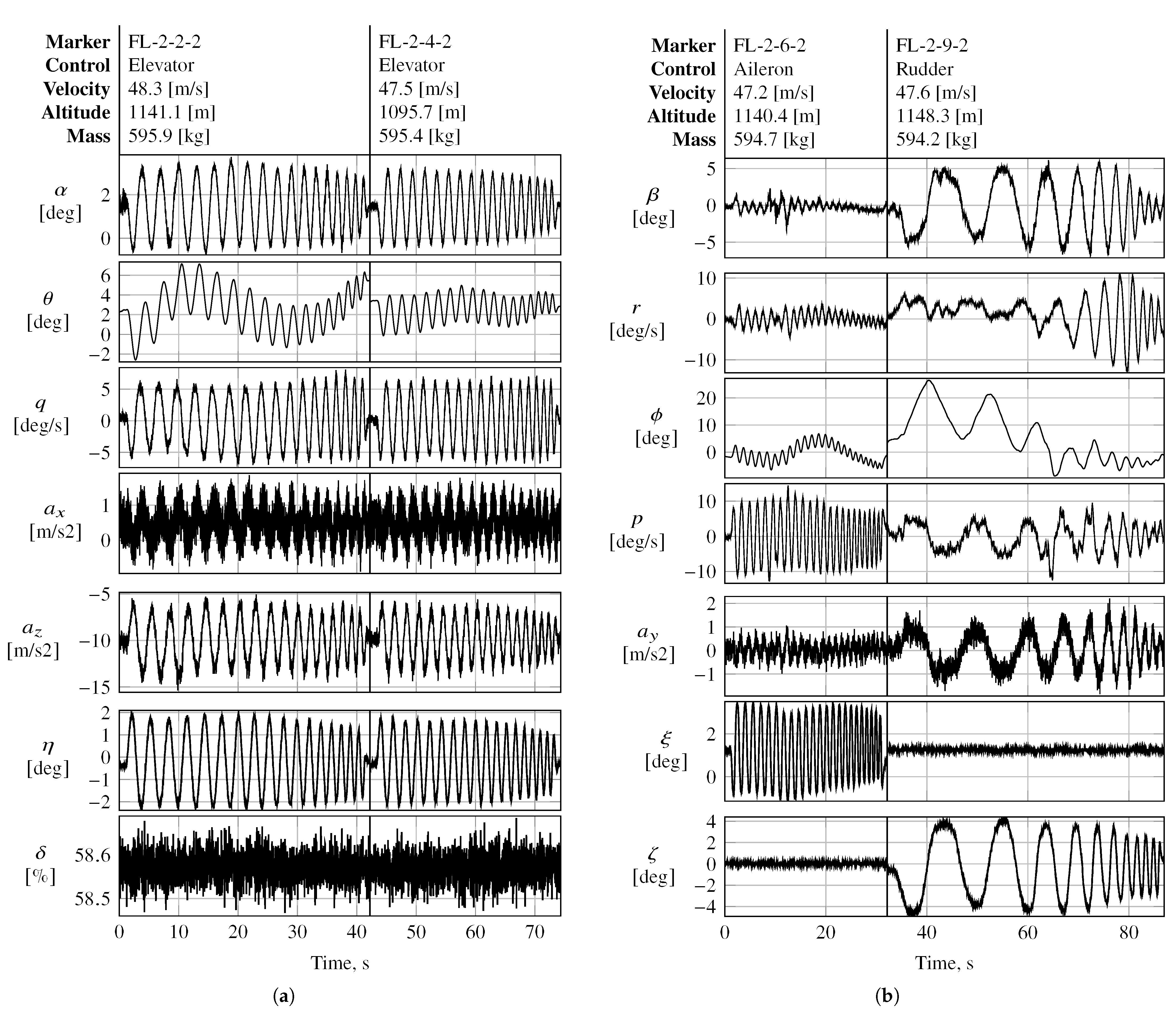
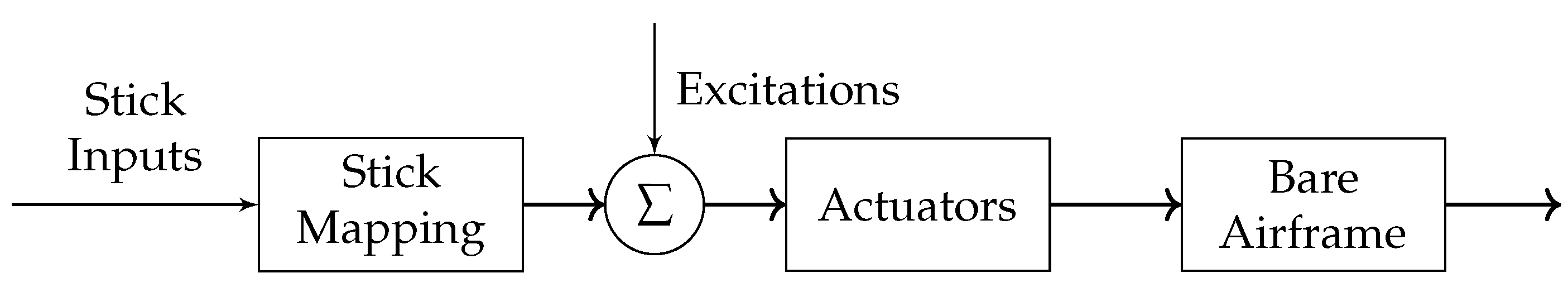
Figure A5 presents the flight data obtained from various longitudinal and lateral frequency sweeps designed to excite the longitudinal and lateral motion of the aircraft, respectively. The sweeps were injected into the elevator, aileron, and rudder separately during steady-state wing-level flight. Unlike the longitudinal sweeps applied to the elevator, the frequency sweeps applied to the aileron and rudder targeted towards the lateral modes of interest, respectively, also excited off-axis rates. 
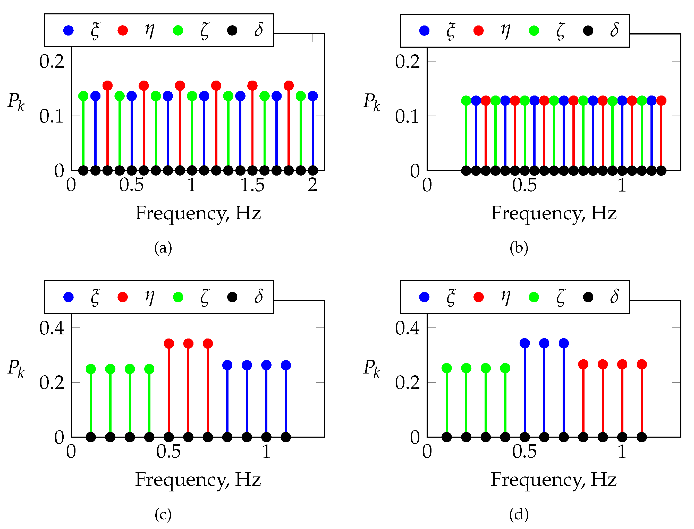
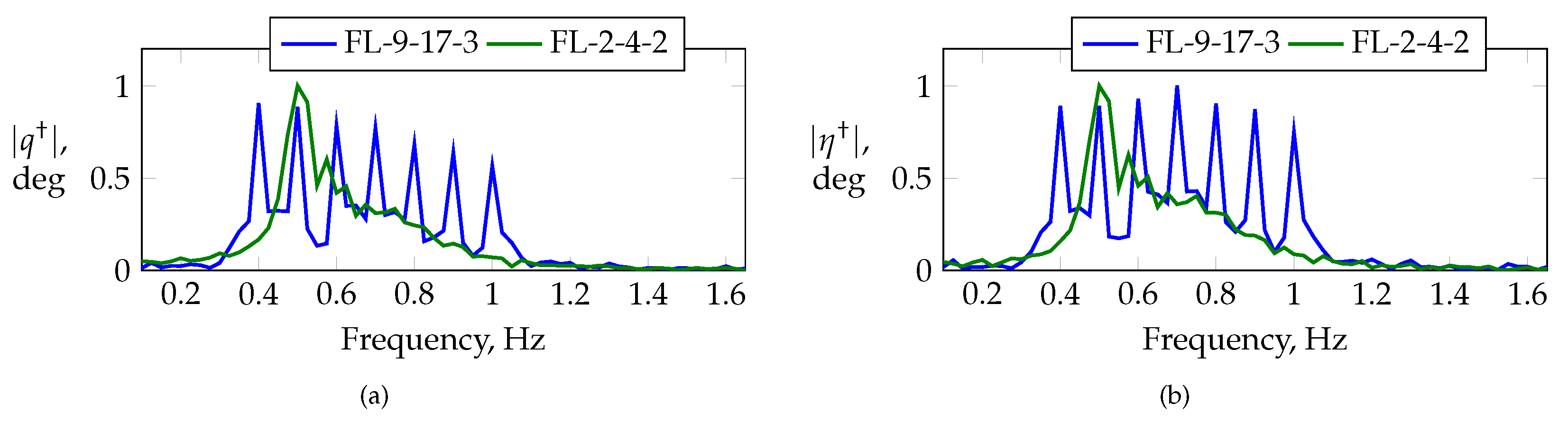
Figure 15 compares the frequency spectra for maneuvers FL-2-4-2 and FL-9-17-3. Maneuver FL-2-4-2 is a linear frequency sweep applied to the elevator, and maneuver FL-9-17-3 is an orthogonal multisine optimized for a low relative peak factor with an alternating frequency distribution among all of the longitudinal control inputs, i.e., the elevator and thrust lever. Both maneuvers were designed to excite frequencies in the vicinity of short-period motion, i.e., frequency bandwidths of [ 0.48 , 0.95 ] Hz for maneuver FL-2-4-2 and [ 0.4 , 1 ] Hz for maneuver FL-9-17-3, with similar control amplitudes of 2 deg of excitation for maneuver FL-2-4-2 and 2.5 deg for maneuver FL-9-17-3. Multisine FL-9-17-3 was designed with a uniform power distribution over all of the control effectors and frequencies, respectively. The frequency range around the short-period region is excited well with both maneuvers; however, higher frequencies are excited better when using the optimized multisine. The latter also clearly excites the discrete frequencies applied by the elevator. A limitation in bandwidth is also visible around 0.7 Hz .
The effectiveness and performance of both maneuvers were compared by estimating a single-point aerodynamic model for the vertical force coefficient C Z
C Z = C Z 0 + C Z α α + C Z α ˙ α ˙ c ¯ 2 V + C Z q q c ¯ 2 V + C Z η η
Both maneuvers had identical excitation times of 30 s and similar input amplitudes and generated similar aircraft responses in terms of the longitudinal explanatory variables. Both maneuvers produced different information content in the frequency domain due to their different input energy distributions—cf. Figure 15—which is why the following analysis was executed in the time domain. The comparison of both inputs, although both have different input energies, is consistent with the argumentation provided in Ref. [1]. The parameters of Equation (14) were estimated using the equation error in the time domain, as described in Refs. [1,3]. Table 7 summarizes the estimation results obtained for both maneuvers, respectively. In addition, the sums of the parameters’ standard errors are provided for both maneuvers. The multisine was shown to provide lower estimation errors for almost all of the parameters, except for C Z 0 . Most of the parameters are in statistical agreement between both maneuvers, except for C Z α ˙ , which is far away from the value obtained using the multisine for the frequency sweep.
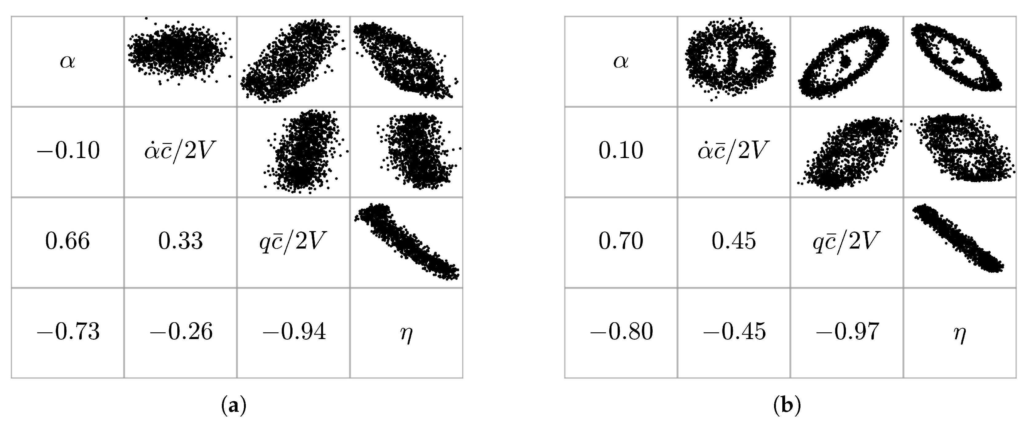
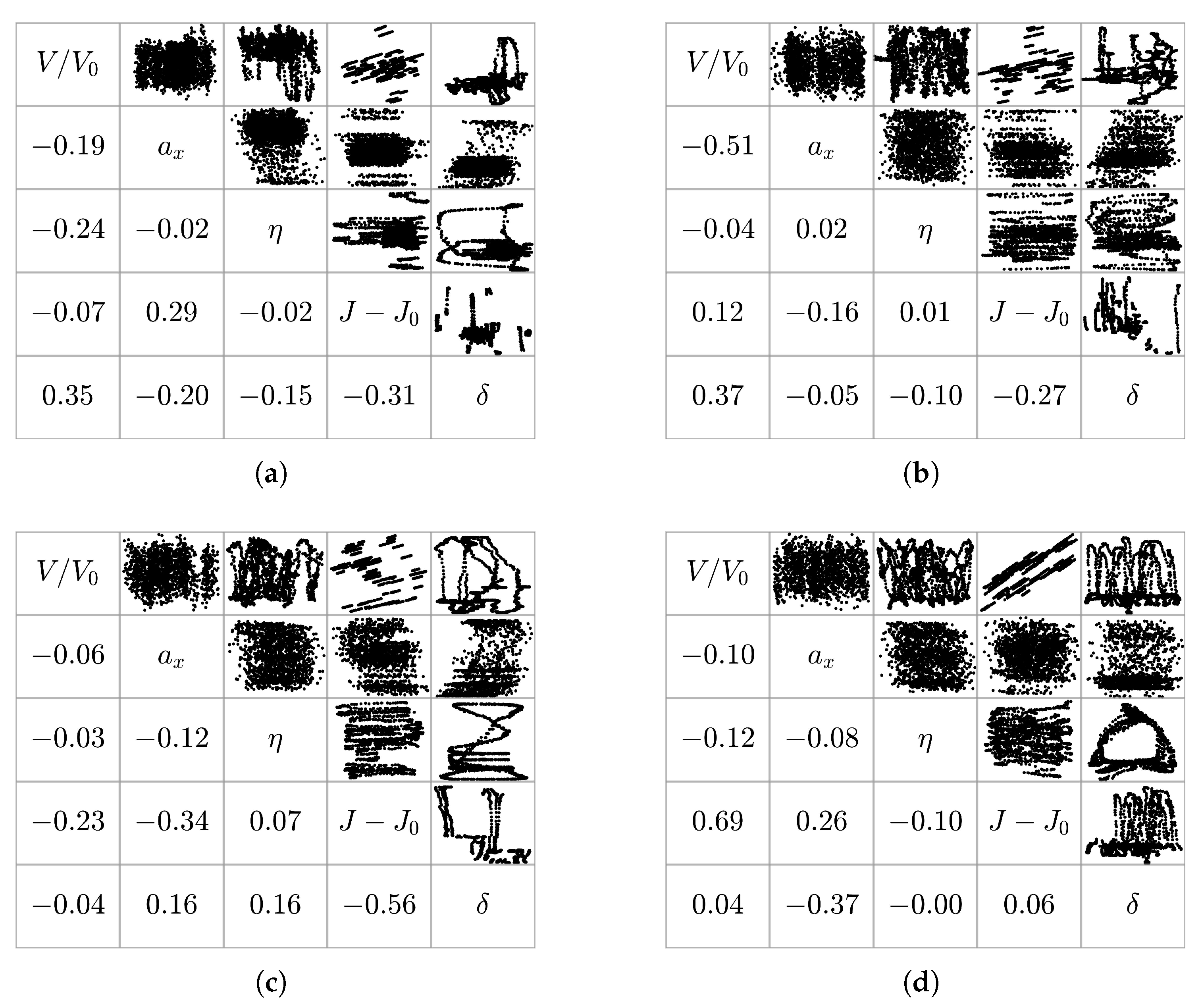
Figure 16 shows the regressor cross plots for both maneuvers, respectively. The multisine maneuver produces pairwise correlation values less than or equal to those obtained with the frequency sweep, while the largest reductions in the absolute pairwise correlation are observed for the regressor pairs α ˙ c ¯ / 2 V q c ¯ / 2 V , α ˙ c ¯ / 2 V η , and α η . Regressors α ˙ c ¯ / 2 V q c ¯ / 2 V are close to the common threshold of 0.9 for the flight data obtained using the frequency sweep.
The low bandwidth of the actuators was also a major issue when using multisteps to excite fast dynamic modes such as the short-period mode. 
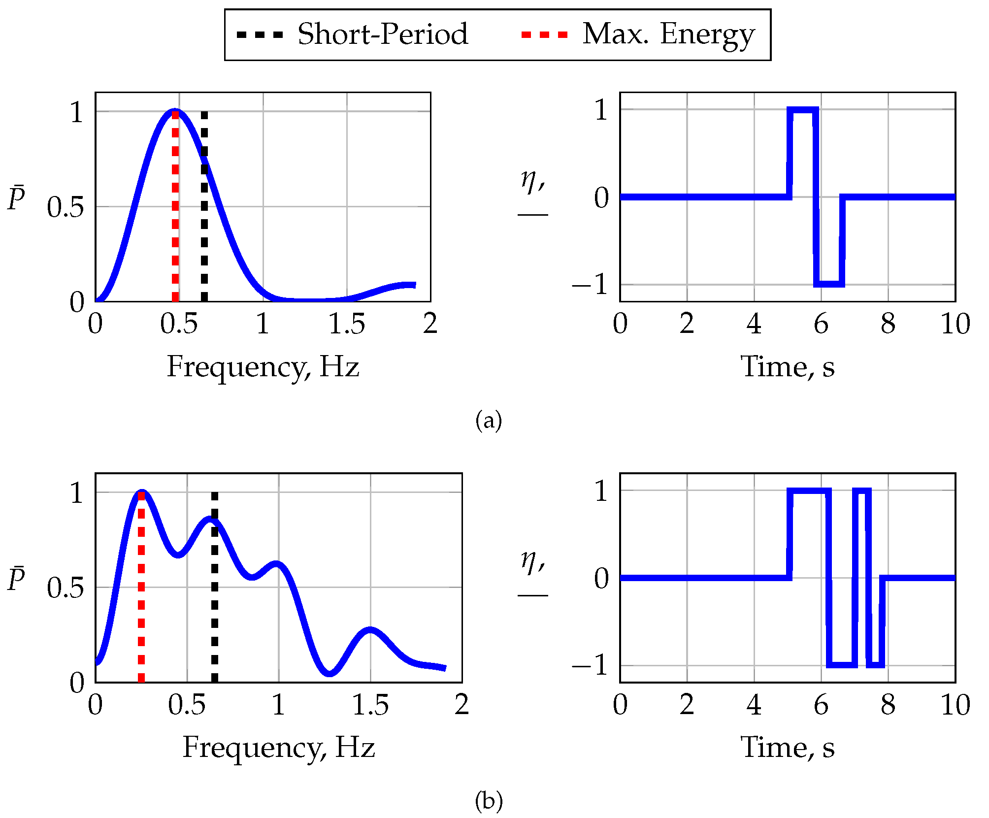
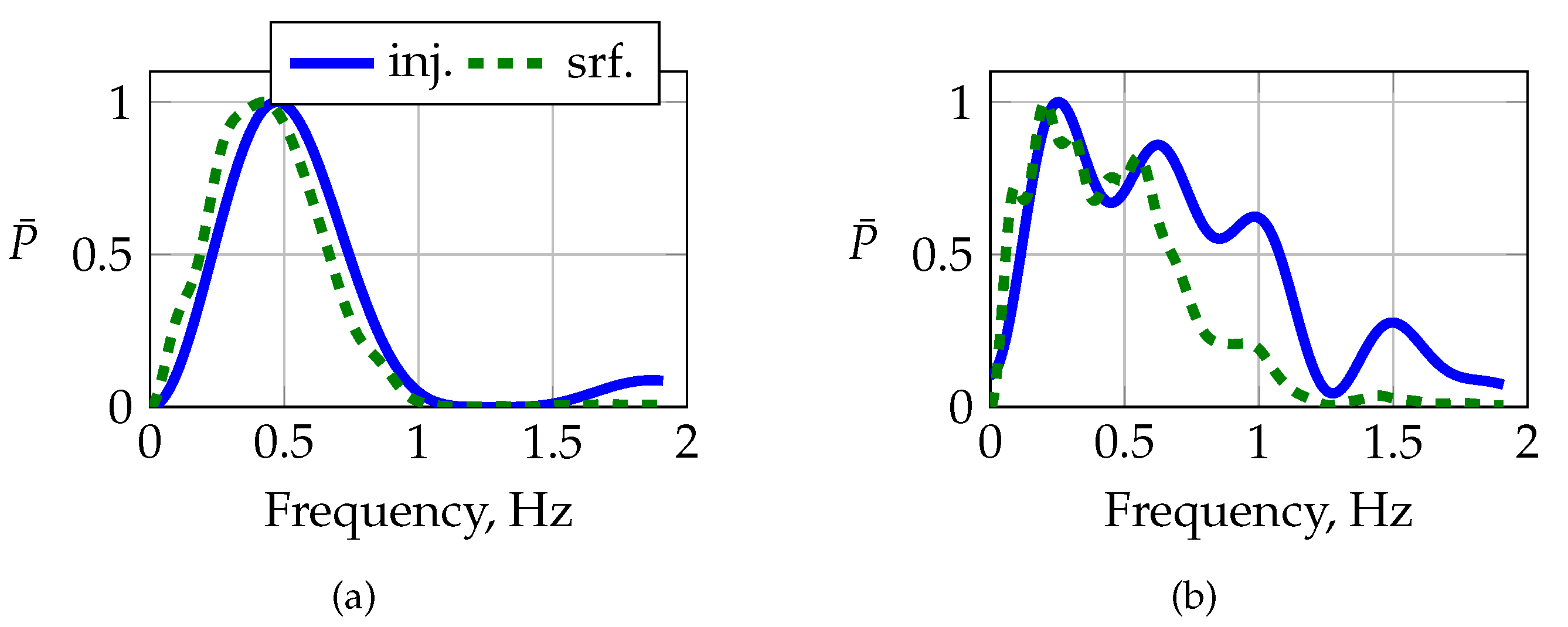
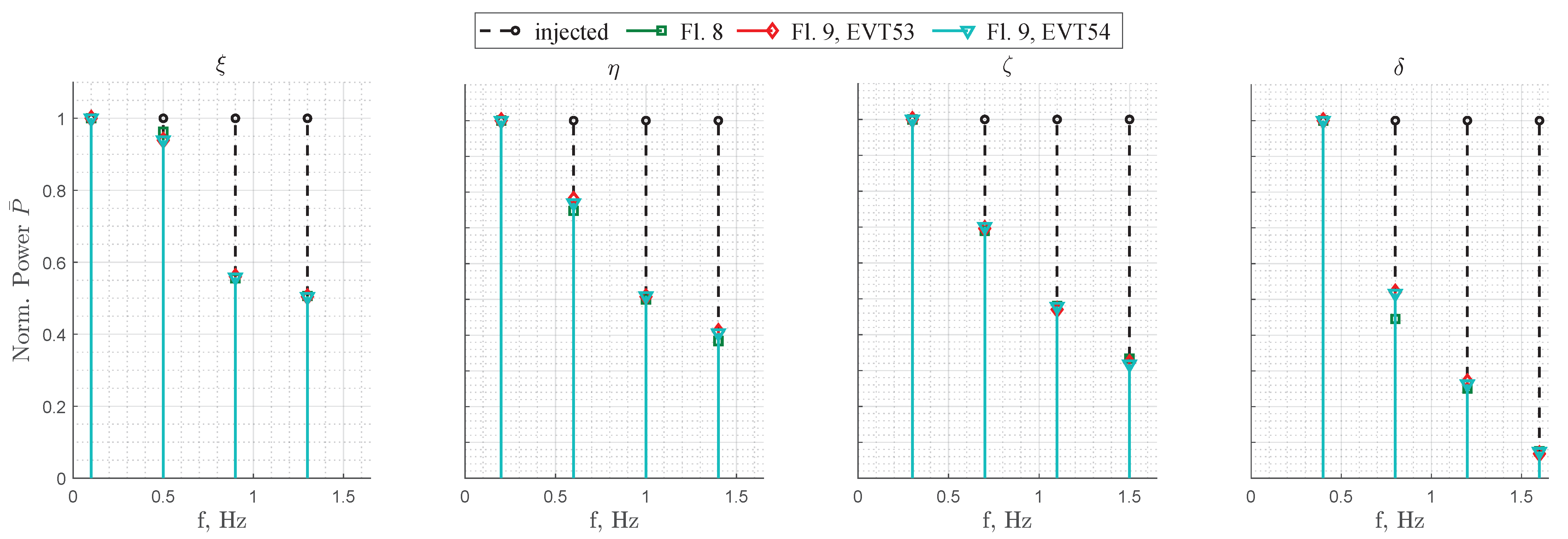
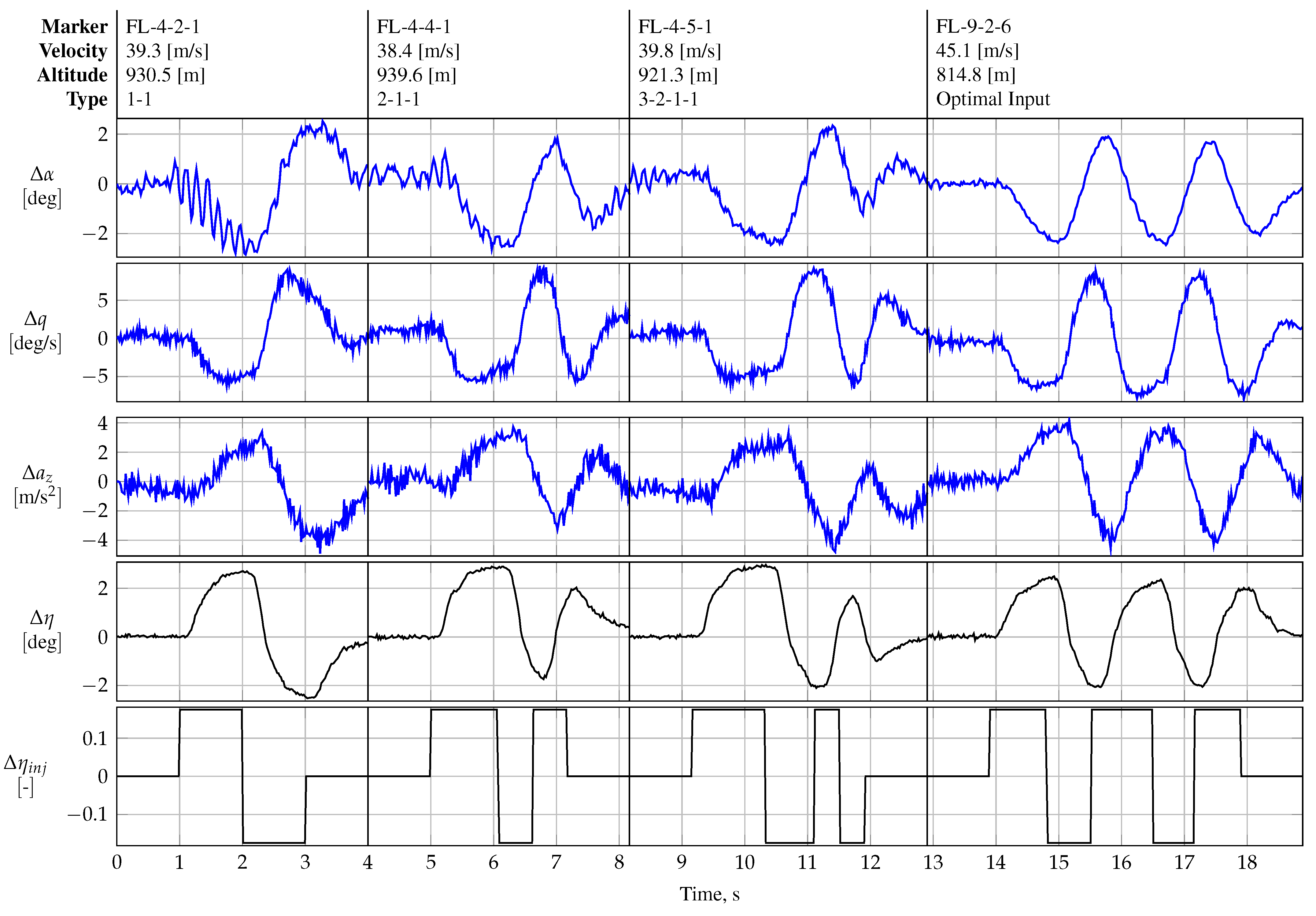
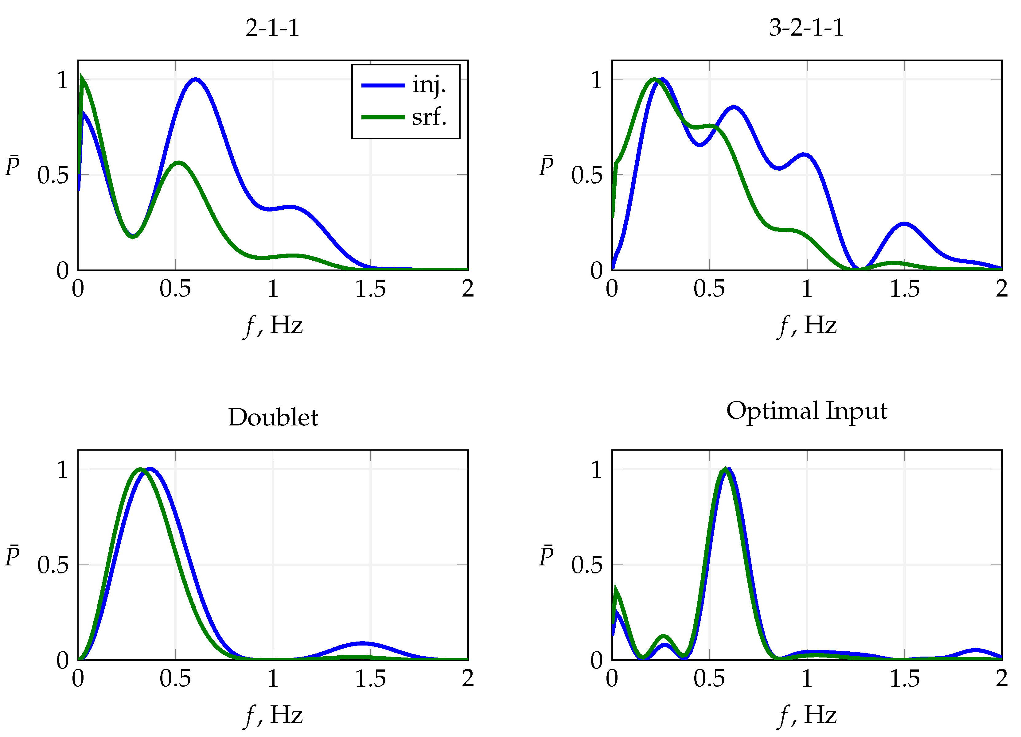
Figure 17 presents the in-flight performance of multistep maneuvers FL-3-1-1 and FL-3-3-1, both designed to excite the short-period mode; cf. Figure 12. Maneuver FL-3-1-1 is a conventional doublet multistep with a fundamental time step of 0.76 s for exciting a short-period frequency of approximately 0.65 Hz . Figure 17 presents the normalized frequency transform of the injected and measured elevator deflections and their respective time histories. The actuator is not able to follow the command properly, indicated by the lagged and alternated surface deflection. Although the actual surface deflection lags behind the commanded deflection, the excited frequency almost matches the target frequency. Maneuver FL-3-3-1 is a 3-2-1-1 maneuver that also targets the short-period mode, with a shorter fundamental step width than that of FL-3-1-1 in order to bracket the short-period frequency with the slower and faster pulse of the 3-2-1-1 sequence. The slow actuator response excites the commanded multistep poorly; cf. Figure 17. The latter is also visible in the sudden drop in the power distribution around 0.6 Hz , which is shown on the left-hand side in Figure 17, which is why the 3-2-1-1 maneuver could not excite the short-period mode at all.
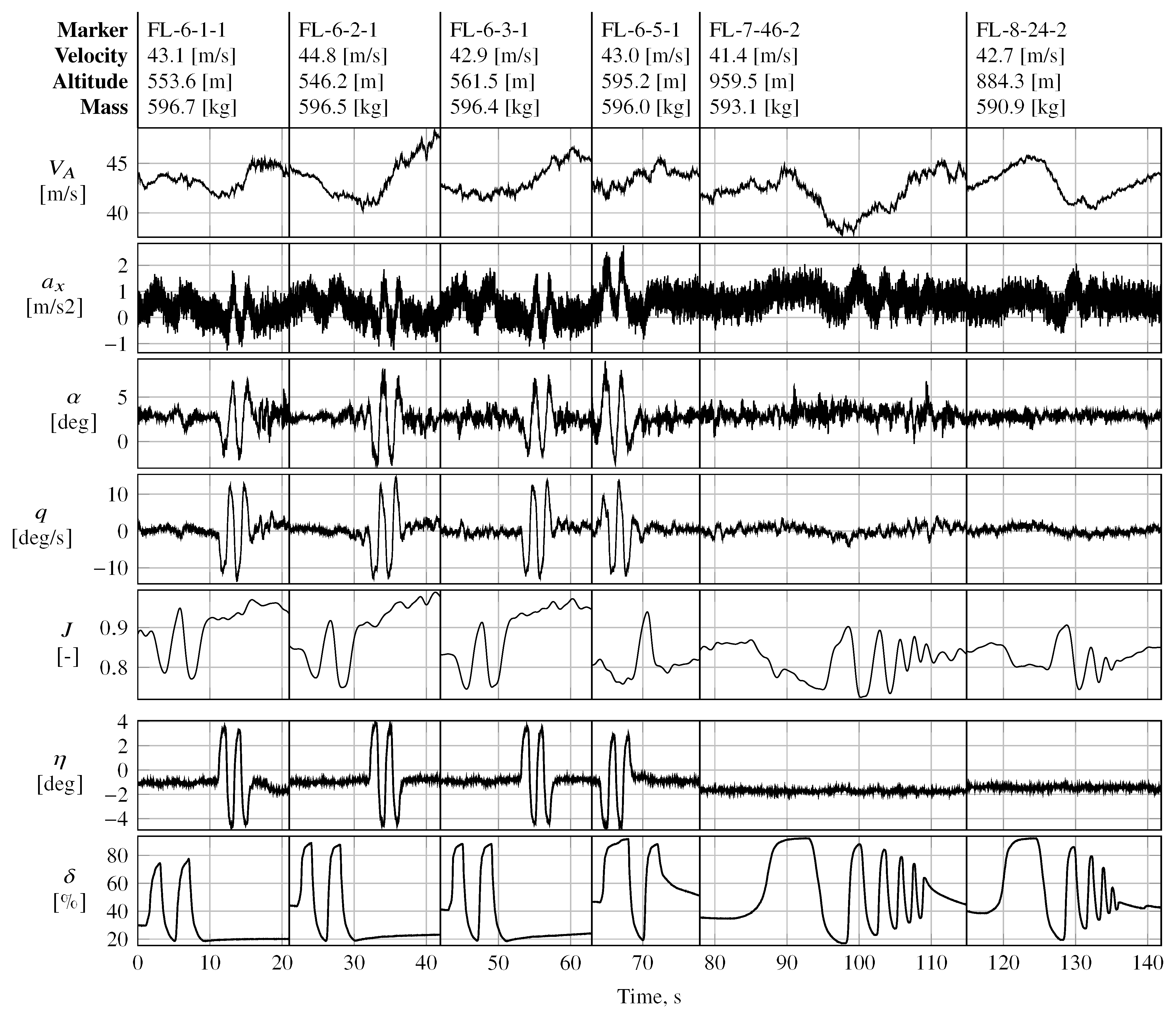
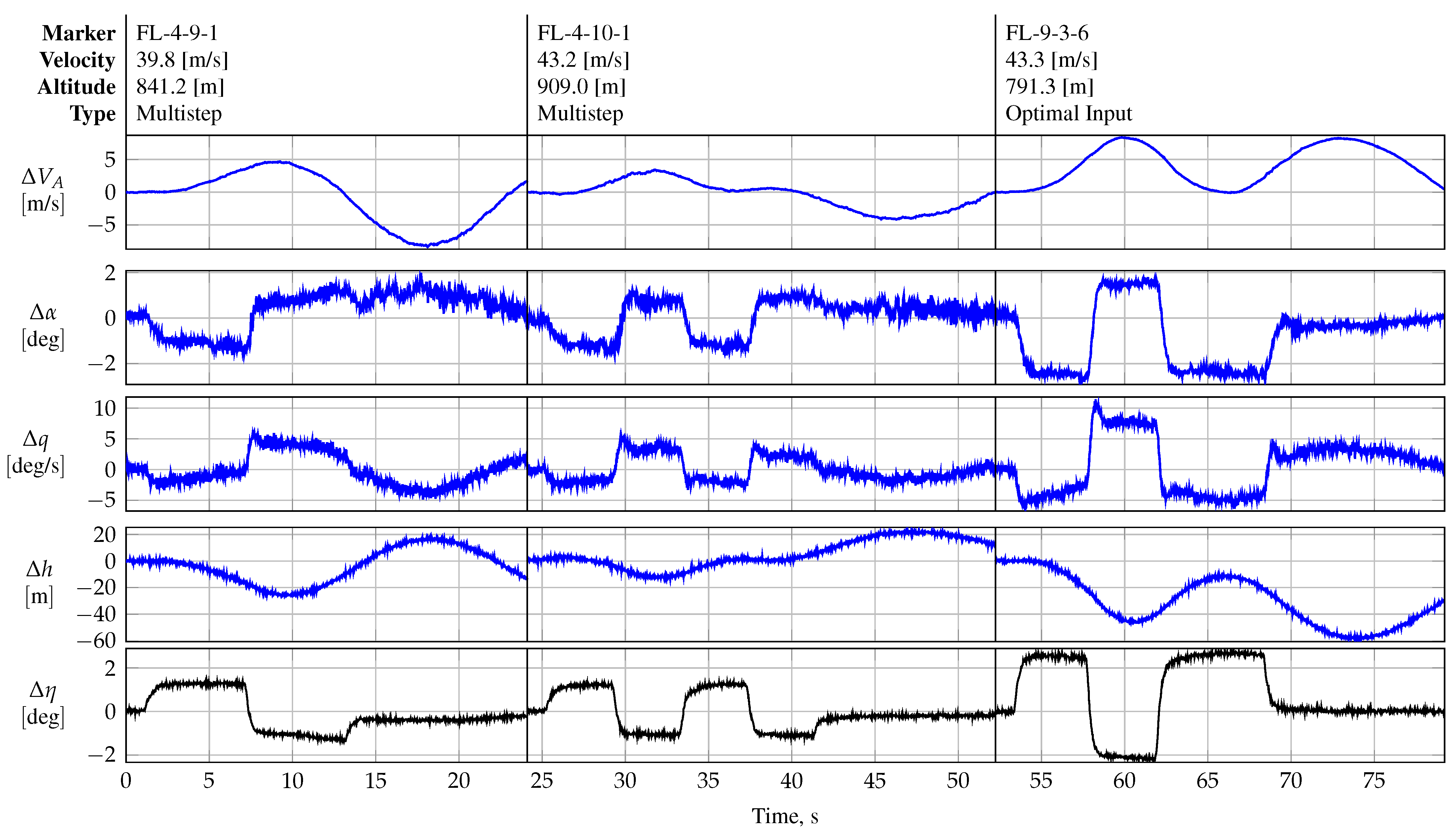
As expected, multisteps performed significantly better in exciting slower dynamic modes, e.g., phugoid motion. Figure 18 shows the flight data obtained after the execution of the FL-4-9-1 maneuver, which was designed to excite phugoid motion in the REMOS GX; cf. Figure 11. Maneuver FL-4-10-1, as shown in Figure 18, is a direct repetition of maneuver FL-4-9-1, with the goal of shifting the maximum injected power to higher frequencies. Both maneuvers excite phugoid motion; however, maneuver FL-4-9-1 performs better than its repeated version.
Multistep maneuvers designed to excite the dominant lateral modes did not result in any loss of the input energy. Figure 19 presents the normalized power spectra for three different orthogonal multisteps applied to both the aileron and the rudder in a time-skewed manner to excite the lateral dynamic modes, e.g., Dutch roll and roll mode. The main reason for the better excitation was that higher frequencies of interest (e.g., roll mode) were assigned to the aileron input, which had a significantly higher bandwidth compared to that of all other actuators, and the designed multistep could therefore be injected properly. Lower lateral frequencies of interest (e.g., Dutch roll) were assigned to the rudder input, which had no difficulties in exciting low-frequency multisteps.
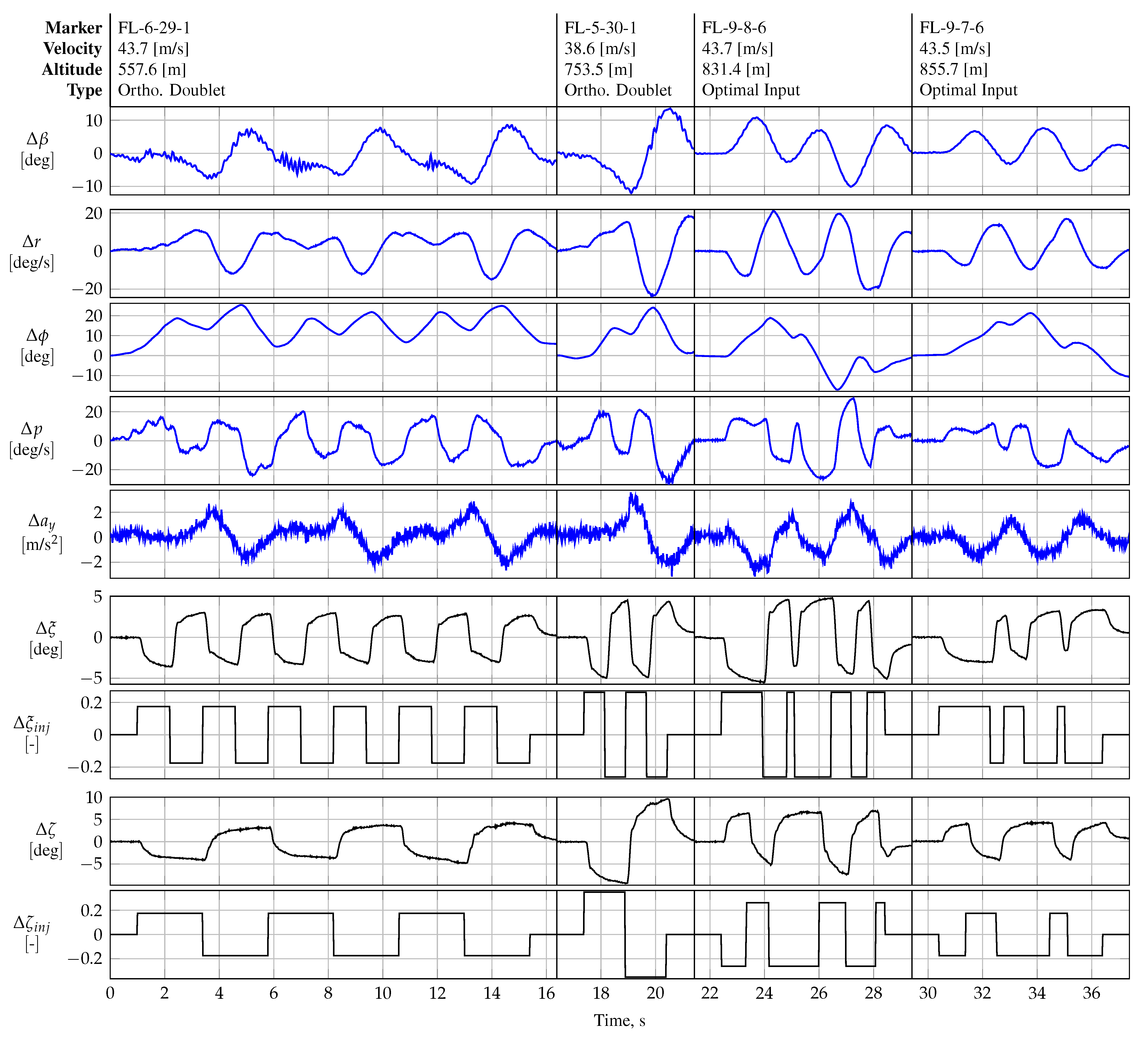
Figure 20 presents the flight data for maneuvers FL-4-23-1, FL-5-30-1, and FL-6-29-1. All three maneuvers presented were designed to be orthogonal to each other in the time domain, i.e., to have an inner cross-product of zero. The longitudinal control effectors (elevator and thrust input) were kept in trim conditions, which is why Figure 20 is reduced to the states for lateral aircraft. In all maneuvers, the duration of the aileron doublet is chosen to match half the duration of one rudder doublet. The time duration and amplitude of both the aileron and rudder inputs were also varied for all three maneuvers. Unlike all other maneuvers, maneuver FL-6-29-1 was designed to shift the maximum input energy to a higher frequency by concatenating each doublet input sequence several times in time, i.e., six times the aileron sequences and three times the rudder sequences, respectively.
All three maneuvers shown in Figure 20 showed low pairwise correlations among the lateral explanatory variables. 
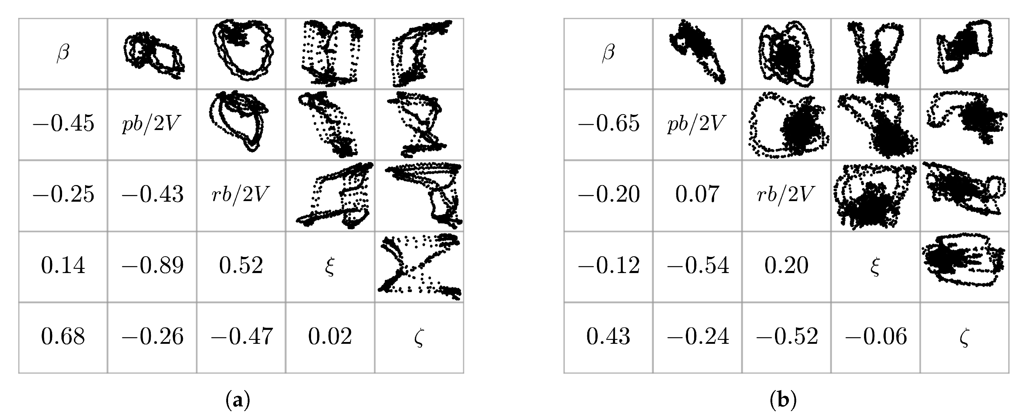
Figure 21 compares the pairwise correlations of the lateral explanatory variables of an optimized orthogonal multisine, designed for the aileron and the rudder only (maneuver FL-9-22-3), with those for the orthogonal multistep maneuver FL-6-29-1. Maneuver FL-9-22-3 was designed to excite roll and yaw motion in the aircraft in the frequency range of 0.05 to 2.00 Hz by manipulating only the lateral controls, i.e., the aileron and the rudder. The atmospheric conditions for both maneuvers were very similar in terms of wind and turbulence levels, producing similar signal-to-noise ratios. The optimized multisine shows lower absolute pairwise correlation values for all lateral regressor pairs. For most of the regressor pairs, however, the pairwise correlation values are similar between both maneuvers. The regressor pairs ξ r, ξ p, and rp show the largest discrepancies between both maneuvers.

5.2. Improvements in the Experiments from Phase 1 Flight Tests

The frequency range used for the phase 1 flight test series was selected to correspond to the frequencies usually associated with the dominant frequencies of conventional aircraft configurations, which usually lie between 0.10 to 2.00 Hz (cf. Ref. [1]). The maneuvers executed during the phase 1 campaign were used to correct and refine the assumptions about the frequencies of the dominant modes of the REMOS GX. The flight test time was critical and limited during phase 1, which is why a fast and top-level analysis of the aircraft’s dynamics was required to improve the excitation of the aircraft. The main analysis is therefore focused on the frequency responses and transfer function estimates. Phase-optimized orthogonal multisines were primarily used to update the initial information about the aircraft’s modes. 
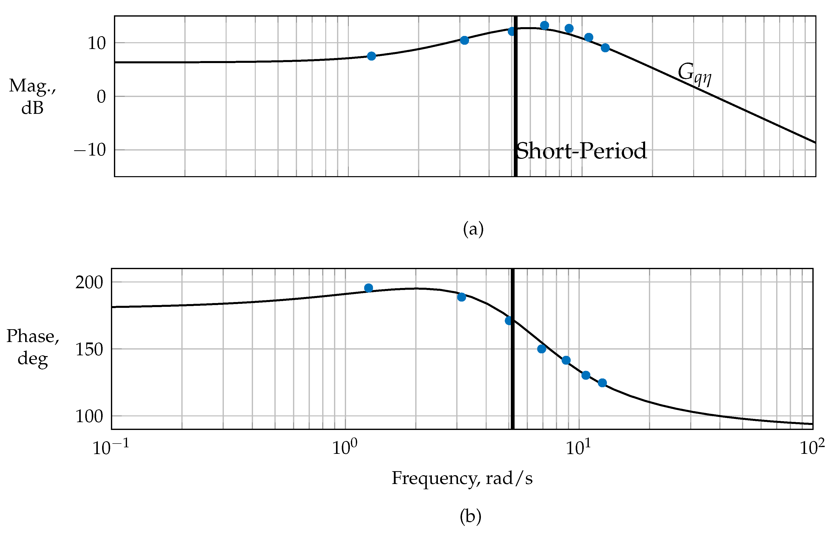
Figure A1 presents several phase-optimized orthogonal multisines designed for aerodynamic modeling (excluding thrust excitation) that were designed using the commonly known frequency spectrum mentioned before. The frequencies were assigned to each control input in an alternating manner, as well as by varying the frequency spectrum for each input, respectively. All maneuvers were designed using a uniform power distribution over all frequencies. Because the maximum number of frequencies was limited to 40 by the maneuver injection unit, the maximum number of frequencies, as well as the finest possible frequency spacing applied to each control effector, was also limited. Further restriction of the maximum and minimum frequency for excitation was therefore required to improve the aircraft’s excitation and the flight data’s information content, especially in the vicinity of the dominant modes. In terms of longitudinal motion, the most difficult mode to excite was the short-period mode. One approach to determining the short period’s frequency was estimating the transfer function between the elevator and the aircraft’s pitch rate. The transfer function from the elevator to the aircraft’s pitch rate is [1]
G q / η = q ˜ η ˜ = K · s + 1 / T θ 2 s 2 + 2 ζ s p ω s p · s + ω s p 2 = b 1 s + b 0 s 2 + a 1 s + a 0
where ω s p is the short-period frequency, and ζ s p is the short period’s damping. The parameters of Equation (15) were estimated using equation error parameter estimation in the frequency domain, following the recommendations provided in Ref. [44]. The parameters estimated for the transfer function G q / η are summarized in Table 8 and correspond to a short-period frequency of approximately 0.89 Hz.
The estimated transfer function was validated against the frequency response estimated from phase-optimized multisines and multisteps from different maneuvers and showed good prediction capabilities. Orthogonal phase-optimized multisines offer various advantages for the computation of frequency responses. Since multisines excite a discrete set of frequencies, there is no need to apply spectral estimation methods that require windowing, averaging, and coherence weighting because the frequency response can be computed at the known excitation frequencies [1,44,57]. Multisines also excite multiple inputs simultaneously (in contrast to frequency sweeps) and therefore reduce the required flight test time significantly. After detrending the explanatory variables in the time domain, the input u i and the output y i are transformed into the frequency domain utilizing the chirp z-transform applied at the known discrete input frequencies of the injected multisine, respectively. The frequency response is then computed from [44]
H i j ( ω k ) = y ˜ i ( j ω k ) u ˜ i ( j ω k )
The magnitude and phase of the estimated frequency response are given by [1,5,44]
| | H i j ( j ω ) | | = 20 log 10 [ H i j ( j ω ) ] 2 + [ H i j ( j ω ) ] 2
H i j ( j ω ) = 180 π arctan [ H i j ( j ω ) ] [ H i j ( j ω ) ]
and are plotted against a logarithmic scale of the frequencies. The components and in Equation (17) are the real and imaginary parts of a complex number, respectively. 
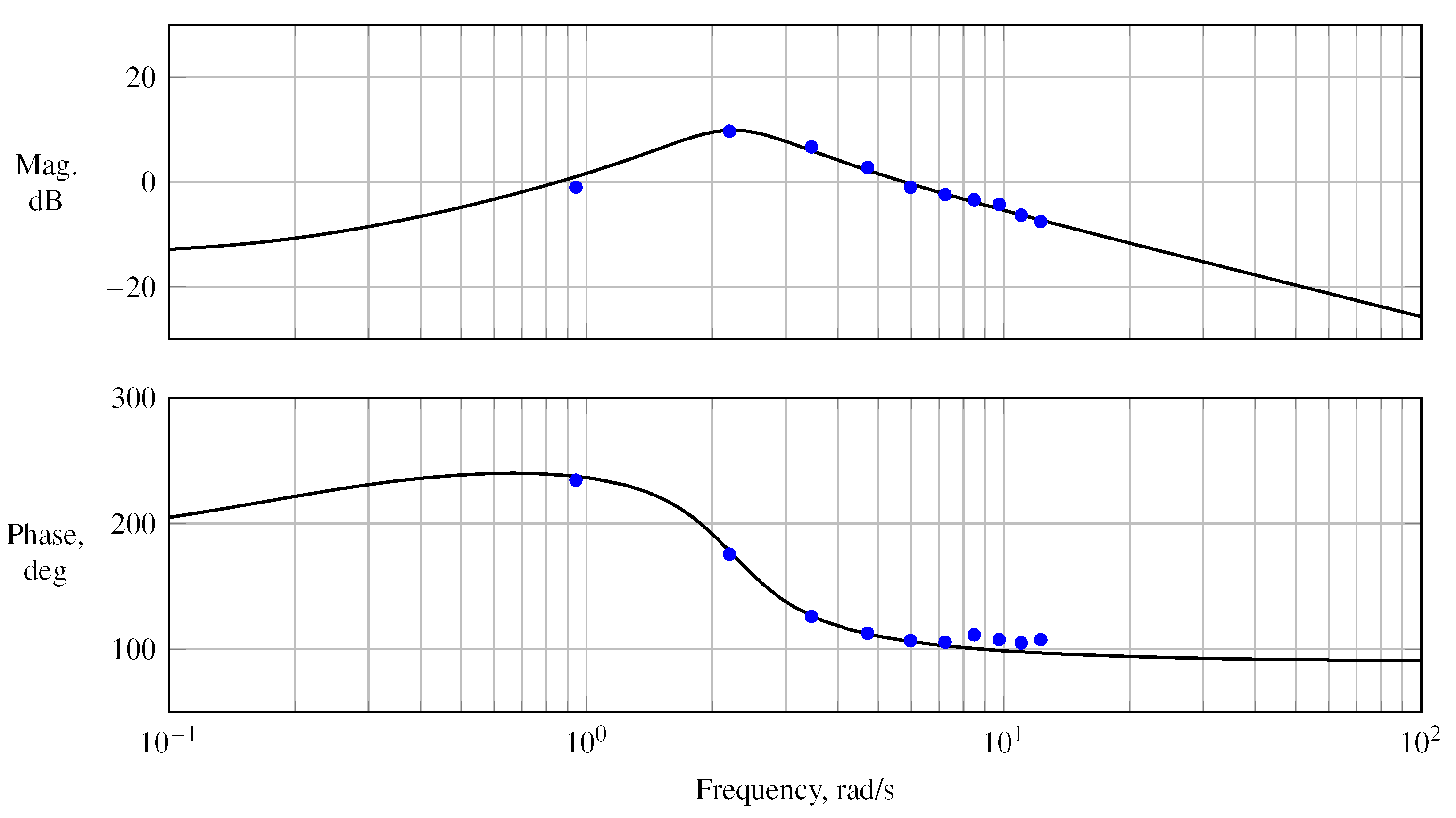
Figure A6 presents the estimated frequency response, magnitude, and phase for the estimated transfer function (cf. Equation (15)). Analogously to longitudinal motion, the same analysis was performed for lateral motion—cf. Figure A4—which yielded the estimated frequency response of the rudder to the yaw rate. Table 9 summarizes the estimated bare-airframe frequencies for the dominant modes used to optimize the maneuvers for the phase 2 flight test series. Since phugoid motion could already be excited very well with the designed multisteps—cf. maneuver FL-4-9-1—no significant update to the phugoid frequency was recognized.
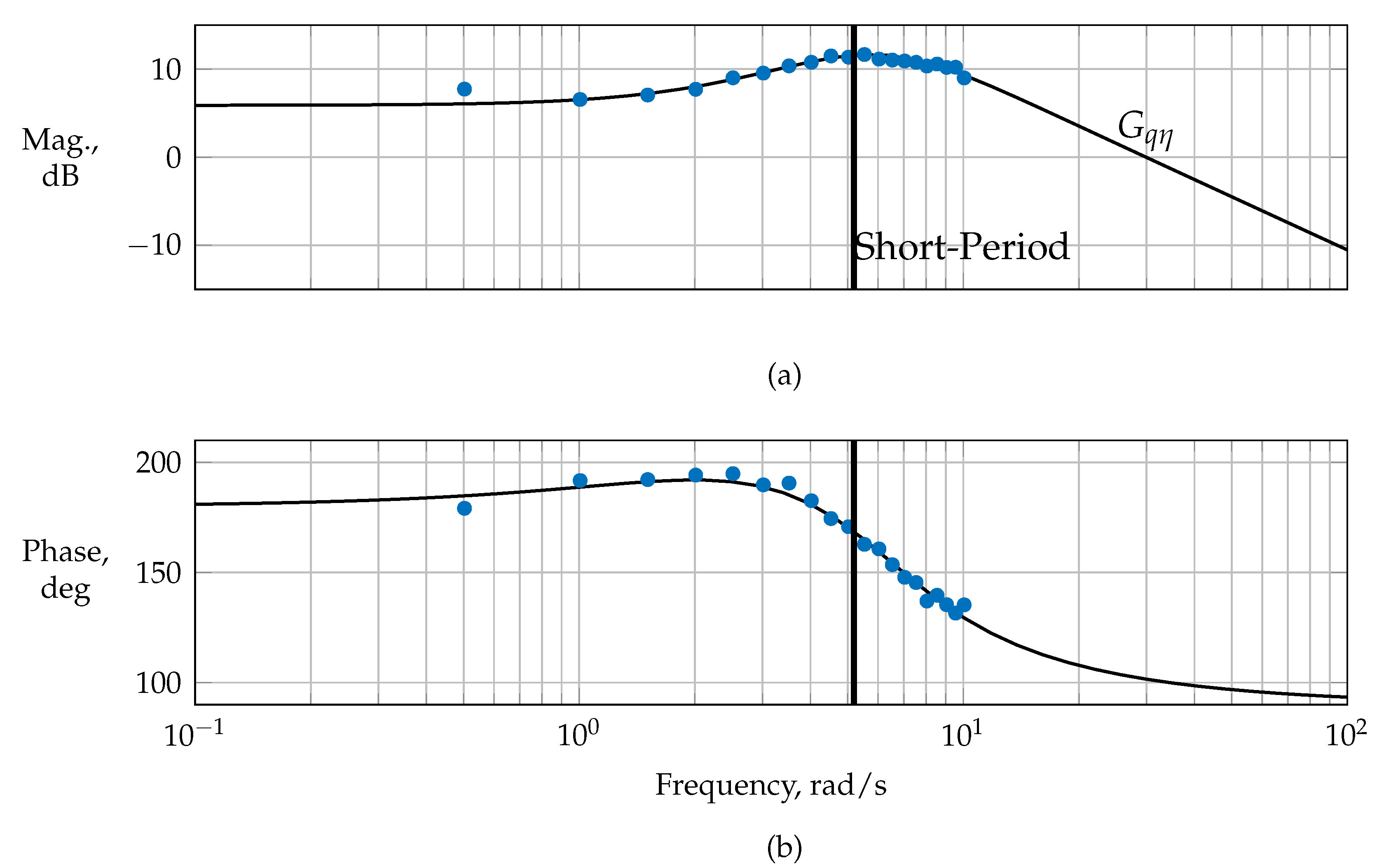
The optimization of maneuvers conducted in preparation for phase 2 focused on varying the excitation frequencies and input amplitudes associated with the maneuvers. The multisines designed for phase 1 were modified by varying the frequency bandwidth and refining the frequency spacing to effectively align the frequencies of interest with the corresponding control effectors. Due to the limitation on the maximum number of frequencies by the injection unit, multisines were also designed for only two control inputs, allowing for a finer allocation of frequencies to each individual control effector. As an example, multisines were also designed for aero-propulsive modeling exciting just the elevator and thrust input. Due to the reduction of control inputs, the frequency spacing could be refined for each input, improving the frequency content near the frequency of interest. Figure A7 shows the estimated frequency response for an optimized multisine applied only to elevator and thrust. The shown input provides a finer frequency spacing around the estimated short-period frequency. In addition, linear models were estimated to further improve information about the frequencies of interest from maneuvers of phase 1. As an example, the short-period model for the REMOS GX was identified using the output error in the time domain. The results were presented in Ref. [34] and are summarized in Equation (19):
α ˙ q ˙ = Z α ( Z q + 1 ) M α M q α q + Z η M η η = 2.54 ( 0.14 + 1 ) 22.86 5.91 α q + 0.23 30.95 η
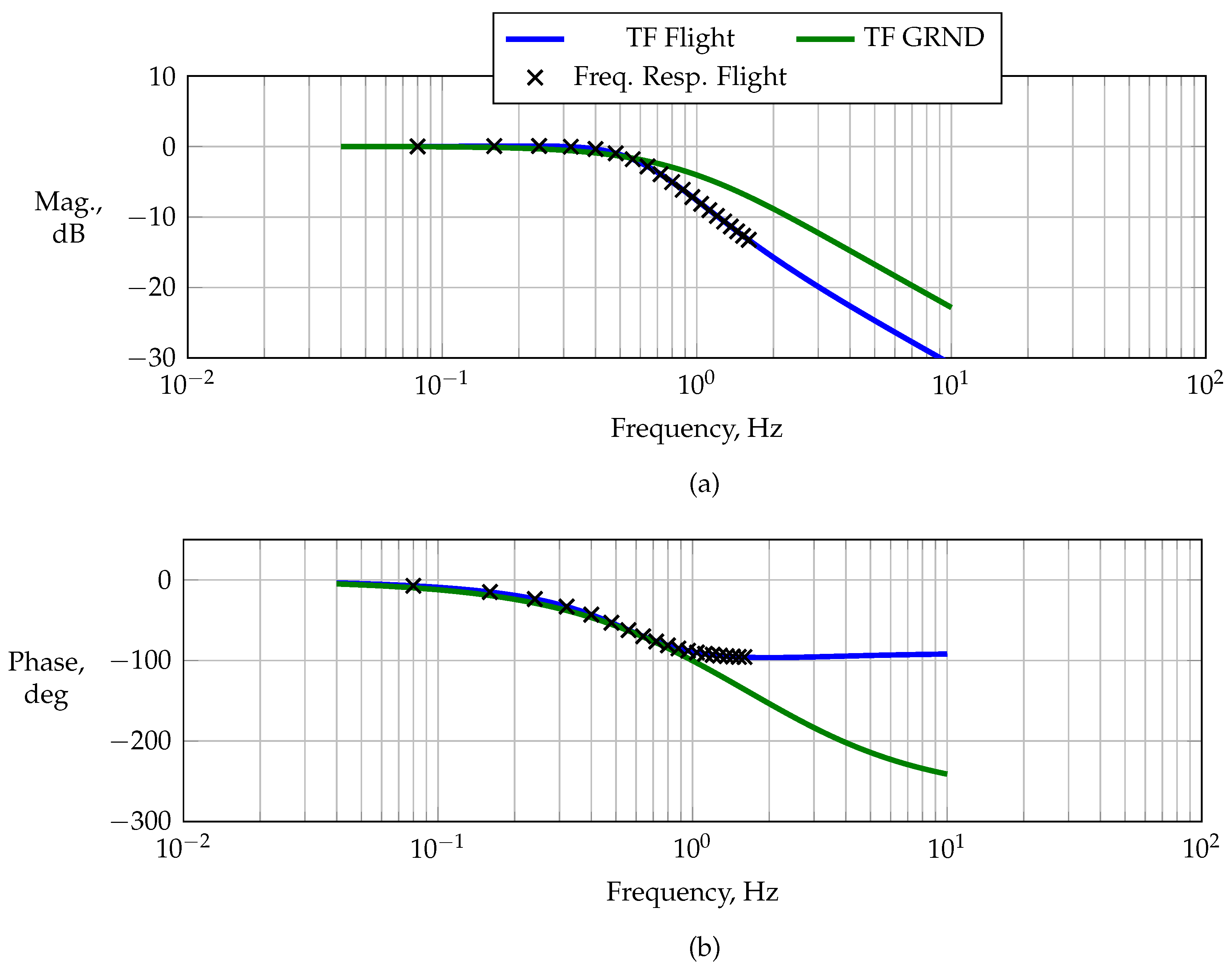
Similar analyses were performed for the dominant lateral modes. The estimation results obtained were used to verify the estimation results based on the frequency responses. Using updated and longitudinal multisines with refined frequencies, the magnitude and phase of q ˙ / η , q / η , and α / η were estimated. 
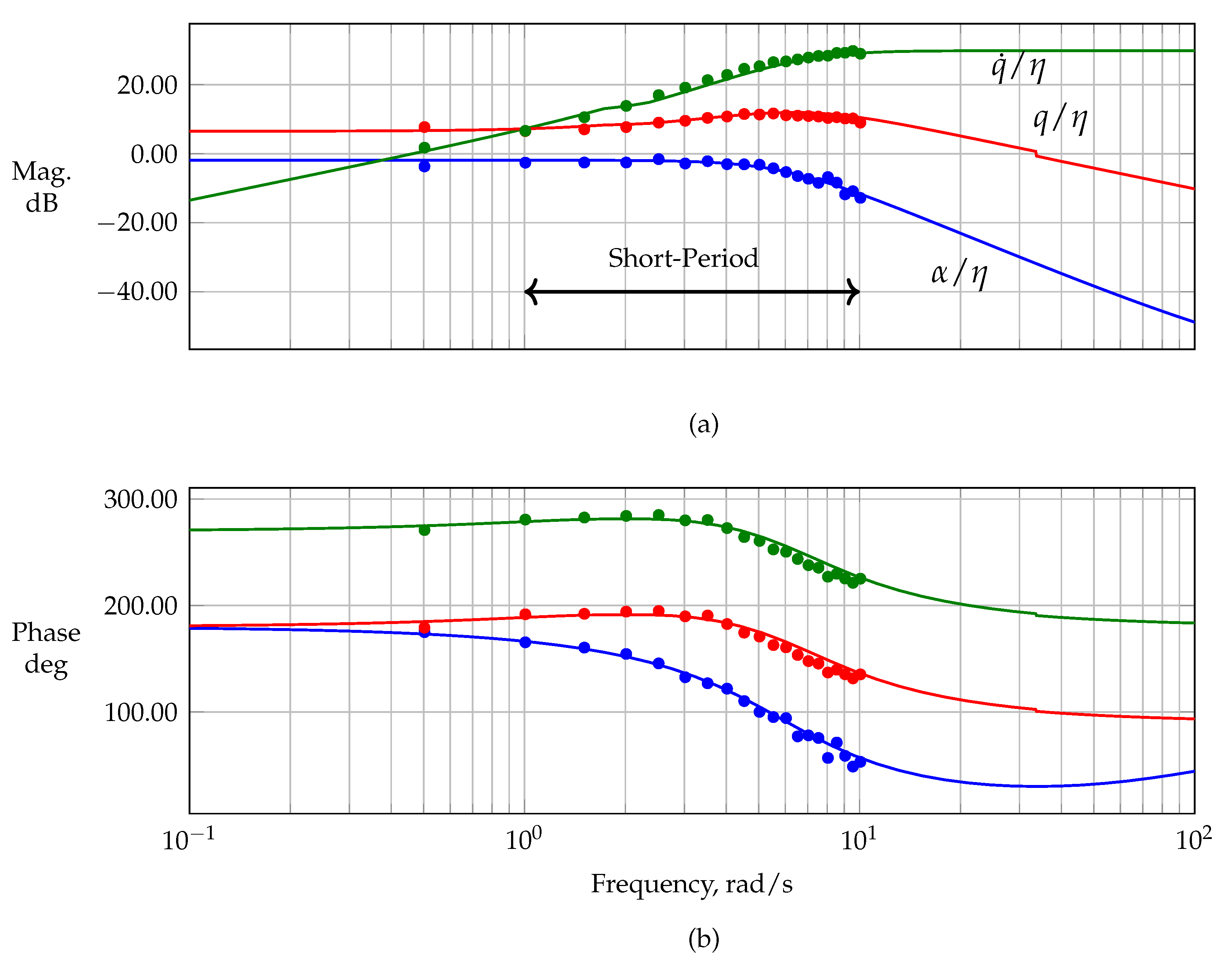
Figure 22 shows the estimated frequency responses against the magnitude and phase obtained from the identified linear short-period model from Equation (19). The short period’s usual frequency range (cf. Ref. [3]) was well covered by the updated refined multisine maneuvers. Although the actuators were limited in bandwidth, which at first degraded the quality of the multisteps for exciting short-period motion and imposed difficulties on its excitation, the multisines provided a good alternative for exciting the short-period mode with an acceptable information content.

5.3. Deterministic Repeatability of the Programmed Test Inputs

The automatic maneuver injection unit provided a significant advantage in executing test inputs designed multiple times under different flight conditions. Figure 23 shows the time histories of the state of the aircraft obtained from a single phase-optimized orthogonal multisine. Each execution was carried out under the same flight conditions. The control deflections show the exact and accurate deterministic repeatability of the designed maneuvers, which could not have been accomplished by a test pilot. The measured angle of attack and the sideslip angle directly show the lower signal-to-noise ratio during flight 8. A comparison of the aircraft’s states reveals that in flight 8, the designed maneuver resulted in a different aircraft response compared to the true airspeed, which is believed to be due to the different c.g. position and mass configuration during that particular flight.
Figure 24 shows the normalized absolute Fourier transform for each control effector injected for the three multisines discussed in Figure 23. The first row of the subplot matrix presents the frequency content of the maneuver executed in flight 8, whereas the remaining two rows show the results for flight 9 at different time steps. The multisine was designed with a uniform power distribution and an identical number of frequencies distributed across all control effectors. It is clearly visible that the injected multisines result in the same frequencies for the measured control surfaces, confirming the accurate repeatability of the designed maneuver. The latter would not have been possible for an experienced test pilot because humans naturally introduce randomness into the applied maneuvers.

5.4. The Actuator Dynamics in Light of External Aerodynamic Loads

Figure 25 shows three different multistep signals, doublet, 2-1-1, and 3-2-1-1, and one optimal input maneuver designed to excite 0.5 Hz in the longitudinal motion of the test aircraft. For all test inputs, the designed signal and the corresponding control surface deflections are shown. The doublet maneuver was designed with a step width of 1 s for each pulse, corresponding to a frequency of 0.5 Hz. Similarly, 2-1-1 and 3-2-1-1 were designed following the respective guidelines of [1,3] to excite the same target frequency. All inputs were designed with an equal input amplitude, while the optimal inputs were designed by considering the actuator dynamics identified during optimization to maximize the information content. More detailed information on the design of the optimal inputs is provided in Ref. [32]. The doublet maneuver was excited very well; however, both the 2-1-1 and 3-2-1-1 maneuvers were not excited properly because the slow actuators could not follow the faster pulse sequences at the end of both maneuvers. The optimal maneuver could, in contrast to all conventional maneuvers, excite each pulse properly because the actuator’s dynamics were considered during the design.
Figure 26 shows the corresponding normalized power spectral density for each maneuver shown in Figure 25. For each maneuver, the designed input spectra and the power spectra computed on the basis of the measured control surface deflection are shown. Both the doublet and the optimal input excite the target frequency; however, the doublet maneuver indicates a significant shift in the maximum input power to lower frequencies. Both 2-1-1 and 3-2-1-1 show degraded input spectra at frequencies of around 0.5 Hz compared to the designed input spectra.

5.5. Maneuvers for Aero-Propulsive Modeling
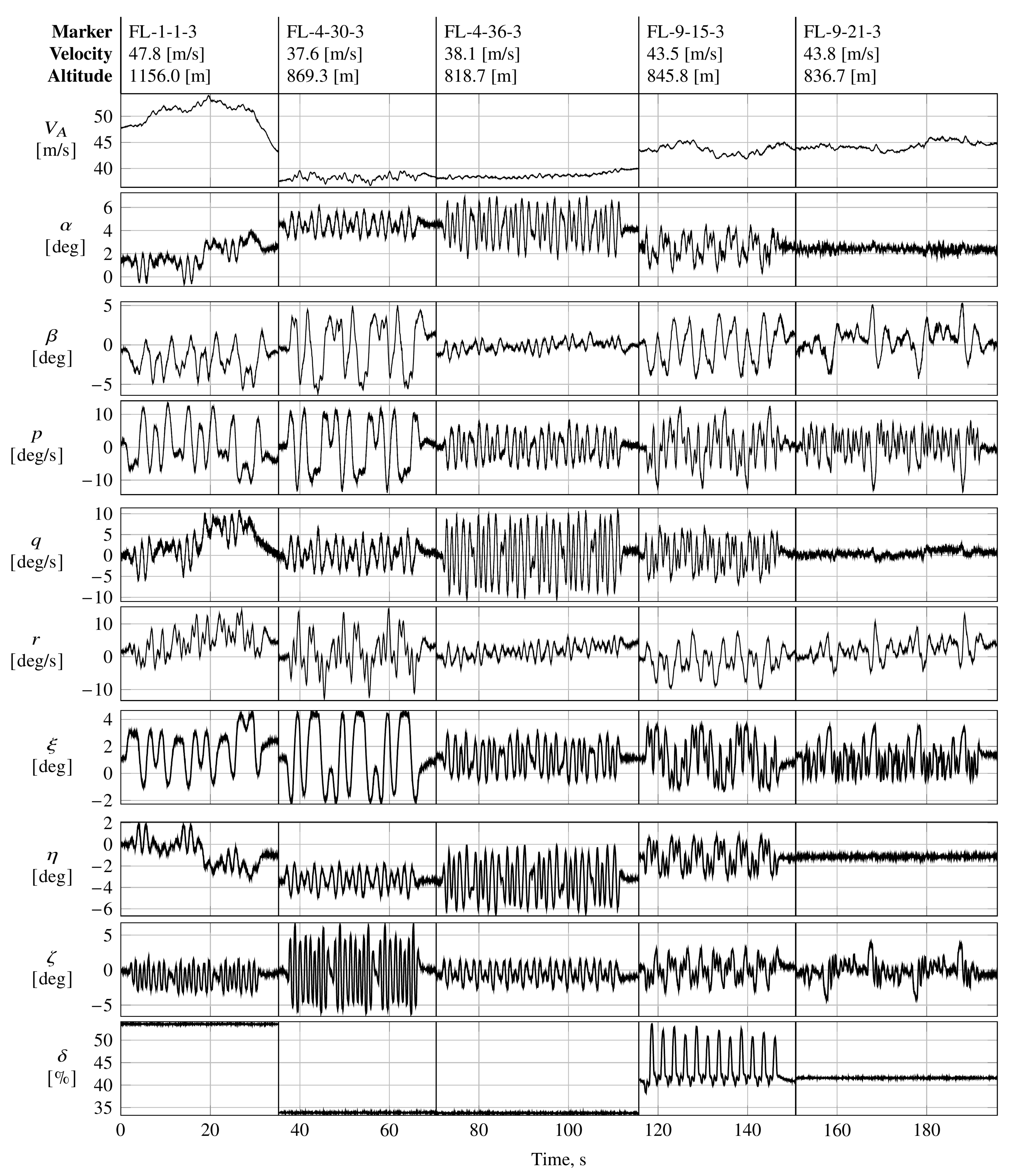
Figure A2 and Figure A3 show the flight data obtained from the frequency sweeps, time-skewed longitudinal multisteps, and phase-optimized orthogonal multisines used for aero-propulsive modeling. The frequency sweeps and optimized multisines were used to identify the propulsive model, whereas the multisteps were used primarily to validate the identified model. The identified model structure, along with the estimated parameter values, is presented and discussed in Ref. [30].
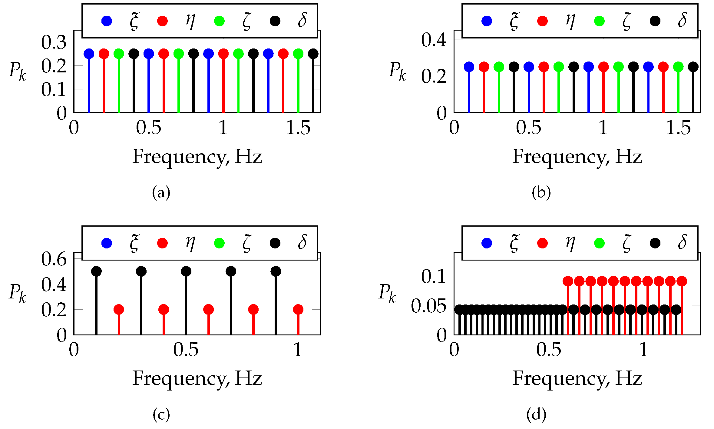
Maneuver FL-9-15-3 was designed as an orthogonal multisine with a conventional consecutive frequency distribution across all of the control effectors excited, i.e., ξ , η , ζ , and δ . This type of multisine was used primarily to identify any possible cross-coupling effects of the longitudinal motion, including the propulsive system with lateral motion. To decouple the longitudinal control effectors more effectively, i.e., the elevator η and the thrust lever δ , several multisines were designed to excite the longitudinal motion only. The frequencies were either assigned in an alternating manner or through simple engineering judgment, as described previously in Section 4.2.4. Maneuvers FL-9-12-3, FL-9-17-3, and FL-9-13-3 are shown as examples of the longitudinal phase-optimized multisines that were used for aero-propulsive modeling. Both maneuvers FL-9-12-3 and FL-9-17-3 were designed using alternating frequencies between the elevator and the thrust lever, whereas maneuver FL-9-13-3 excited the low-frequency spectrum only in the thrust lever channel. Maneuvers FL-9-12-3, FL-9-13-3, and FL-9-17-3 were designed to excite the longitudinal control inputs only, whereas FL-9-15-3 was designed to excite all controls. Maneuvers FL-9-13-3, FL-9-15-3, and FL-9-17-3 had a fundamental period of 30 s, respectively, while maneuver FL-9-12-3 was designed with a period of 50 s, reducing the frequency spacing of the frequencies excited; cf. Figure 13. All maneuvers had roughly the same frequency bandwidth. All multisines shown were designed with different power spectra among the control effectors. In general, higher frequencies above 1 Hz were avoided for the thrust lever channel in order to minimize the total load acting on the engine and the propeller. Furthermore, lower frequencies applied to the thrust lever also resulted in a better response from the aircraft with respect to the injected input.
Input design metrics, e.g., the relative peak factor, the pairwise absolute correlation, and the variance inflation factor, quantify the efficiency and quality of a dynamic test input for exciting the system under test for system identification and parameter estimation. Figure 27 presents the evolution of the commonly used input design metrics against time. Among others, the relative peak factor, the maximum absolute variance inflation factor V I F j , the maximum absolute pairwise input correlation, and the condition number of the input matrix U T U are shown as a function of time for the different multisine designs designed for dynamic aero-propulsive modeling. All of these metrics were computed based on the actual measured control inputs. The relative peak factor of a signal u j is defined as [1]
RPF = max ( u j ) min ( u j ) / 2 u j T u j / N
and quantifies the ratio of the input signal’s amplitude range to its root mean square value, normalized to the peak factor of a single-frequency sinusoidal signal [1,58]. For system identification, an RPF value close to one is desirable, as this helps to keep the system close to its reference flight conditions [51]. Low RPF values lead to a diminished peak-to-peak amplitude in the multisine excitation, consequently limiting the achievable temporal gradients of the signal. Mutual orthogonality remains unaffected regardless of the phase angles selected for the minimum RPF [2]. However, due to the actuator dynamics, mutual orthogonality of the measured control inputs is not guaranteed. The correlation between two signals can be assessed using the pairwise correlation coefficient r j k [1,3]
r j k = i = 1 N x j ( i ) x ¯ j x k ( i ) x ¯ k i = 1 N x j ( i ) x ¯ j ( i ) 2 i = 1 N x k ( i ) x ¯ k ( i ) 2
where x ¯ j and x ¯ k are the mean values of the j-th and k-th regressors, respectively. As an alternative to the pairwise correlation coefficient, the variance inflation factor, defined as the diagonal elements of the U T U 1 matrix, can be investigated [1]:
V I F j = 1 1 R j 2
where R j 2 is the coefficient of determination of the regression of the j-th regressor, modeled as a linear function of all of the other regressors in the model [1]. A V I F j value of 1 indicates no correlation between the j-th regressor and all other regressors, whereas a V I F j value greater than 10 indicates high correlation, which is, however, always database-dependent [1]. The pairwise correlation r j k and V I F j can only be used to assess the correlation among two regressors and can therefore not guarantee that collinearity among more than two regressors is not present because mutual collinearity can be masked by other regressors. To address this shortcoming, the condition number κ , defined as the ratio of the maximum to the minimum eigenvalue of the input matrix U T U , can be used [1,59]:
κ = max e i g ( U T U ) min e i g ( U T U )
This is used to identify collinearity issues among the columns of U. A value of κ near one suggests low multicollinearity, while a high κ value indicates a poorly conditioned estimation problem caused by collinearity. Depending on the dataset, κ values between 100 and 100,000 are considered problematic [1,58].
The maximum absolute pairwise correlation for all control effectors as a function of time is shown in Figure 27a. For all multisines, the maximum absolute pairwise correlation values show a similar trend of decreasing toward low absolute correlation values. All multisines achieve a low correlation value after approximately 25 s, independent of their fundamental base period and frequency distribution. The maximum relative peak factor is shown in Figure 27b. All multisines show a comparable trend of increasing slightly toward their designed peak factor. In summary, all multisines show acceptable peak factors around or below 1.5 after approximately 10 s. The maximum variance inflation factor V I F j is shown in Figure 27c. Only the two multisines with the highest base periods and the lowest frequency ranges achieve an acceptable maximum V I F j value. All of the other multisines show significantly higher values, which is believed to be due to the sluggish response of the servo manipulating the thrust channel. The condition number of the input matrix U T U is shown in Figure 27d. All test inputs converge to a constant condition number of approximately 100 or lower after approximately 10 s. Maneuvers FL-6-39-3 and FL-9-13-3 exhibit, in general, the lowest condition number of approximately 10. The condition number continues to decrease for all test inputs. In summary, optimized multisines with a lower frequency content and higher base periods revealed superior input design metrics for aero-propulsive modeling. Furthermore, guided by the results of this time-dependent analysis and corroborated by previous studies that have demonstrated the efficiency of an enhanced frequency spacing [58,59], multisines with higher fundamental periods were selected for aero-propulsive modeling.
Figure 28 shows the final cross plots of the propulsive explanatory variables for each maneuver, respectively. In general, all of the multisines showed good pairwise correlations among the aero-propulsive explanatory variables. Although the amplitude applied to the thrust lever was lower than that for the other maneuvers, maneuver FL-9-15-3 showed the best capability to decorrelate both longitudinal control effectors, which might be related to the fact that the propulsion system could respond to lower frequencies better with coarser frequency spacing. All of the other maneuvers discussed also showed acceptable correlation values but were designed with a finer frequency spacing, which meant they could not be excited precisely by the sluggish propulsion system.

6. Concluding Remarks

Automatic maneuver injection was implemented on a general aviation aircraft to produce flight data rich in information, facilitating system identification and parameter estimation. These maneuvers were introduced into an open-loop configuration under diverse flight conditions spanning the aircraft’s operational envelope. The test aircraft, a REMOS GX possessing a maximum take-off weight of 600 kg, is a comprehensively instrumented research aircraft that is employed for the evaluation of bespoke flight control systems. The findings highlight several key lessons that are critical for the design and execution of similar experimental campaigns. First, it is essential that the actuator linkage designs avoid any form of kinematic singularity. Such singularities can lead to mechanical jamming, restricting the motion of the control surfaces and compromising the pilot’s ability to provide timely corrective inputs. Ensuring smooth and continuous kinematic behavior is fundamental to both safety and control fidelity. Second, the actuator selection must consider the pilot’s override capabilities. In this study, relatively weak actuators were chosen to allow for manual overriding at all times. Alternatively, actuators should be equipped with dedicated fail-safe mechanisms such as clutches or shear pins to satisfy the aviation safety requirements. This consideration is especially important in manned flight tests, where system failures must not compromise controllability. Power management was identified as another critical aspect. The electrical system on board light general aviation aircraft may not be able to reliably support the additional load imposed by the actuators. Therefore, the provision of a separate, dedicated power supply is strongly recommended to ensure consistent actuator operation throughout the test campaign. In addition, significant discrepancies were observed between the actuator’s performance on the ground and in flight. Specifically, the actuator dynamics were noticeably slower in the airborne environment. This behavior, which aligns with the findings reported for smaller aircraft in Ref. [35], underscores the importance of characterizing the actuator behavior under actual flight conditions rather than relying solely on ground-based assessments. Given the actuator’s dynamic limitations and the lack of steady-state accuracy, direct measurements of the control surface deflections proved to be vital. These measurements enabled accurate tracking of the actual control inputs delivered to the aircraft, which was essential for validating the excitation maneuvers and ensuring the integrity of the identification procedures for the system. Finally, a cautious and incremental approach to maneuver injection is strongly advised. Beginning the flight test campaign with low-amplitude, broadband excitations, such as multisine signals, allowed for initial system characterization with minimal risk. This strategy provided valuable information on the dynamic behavior of the aircraft and helped inform the design of subsequent higher-amplitude maneuvers. Together, these insights contribute to a broader understanding of the practical challenges and best practices in maneuver injection for system identification for light sport general aviation aircraft. Future work may expand upon these findings by exploring adaptive control strategies and more advanced actuator technologies to enhance the test efficiency and safety further.

Author Contributions

Conceptualization: R.K.H. and B.H.; methodology: R.K.H.; software: R.K.H. and B.H.; validation: R.K.H.; formal analysis: R.K.H.; investigation: R.K.H.; resources: R.K.H. and B.H.; data curation: R.K.H. and B.H.; writing—original draft preparation: R.K.H.; writing—review and editing: R.K.H., B.H. and F.H.; visualization, R.K.H.; supervision: F.H.; project administration: B.H. and F.H.; funding acquisition: F.H. All authors have read and agreed to the published version of the manuscript.

Funding

The flight data used in this work was funded by the federal government of Germany as part of the LuFo program (funding ID: 20Q1719D).

Institutional Review Board Statement

Not applicable.

Informed Consent Statement

Not applicable.

Data Availability Statement

The dataset is available on request from the authors.

Acknowledgments

The help and support of messWERK GmbH, in particular Matthias Cremer and Björn Brandt, during the flight test campaign of AMIGAA are greatly acknowledged.

Conflicts of Interest

The authors declare no conflicts of interest.

Abbreviations

The following abbreviations are used in this manuscript:
a x , a y , a z body-axis translational accelerometer measurements, m / s 2
p , q , r body-axis roll, pitch and yaw rate, rad / s or deg/ s
ϕ , θ , ψ euler roll, pitch and yaw angle, rad or deg
η , ξ , ζ elevator, aileron, rudder control surface deflections, rad or deg
bwing span, m
c ¯ mean aerodynamic chord, m
S r e f wing reference area, m 2
maircraft mass, k g
α , β angle of attack, sideslip angle, rad or deg
q ¯ dynamic pressure, N / m 2
θ vector of model parameters
ggravitational acceleration, 9.80665 m / s 2
L P engine power, k W
laircraft fuselage length, m
haltitude, m
ttime, s
TManeuver length, s
P k power spectrum
P ¯ normalized power spectral density
ω , ffrequency, rad or Hz
dBdezibel
degdegree
Mag.magnitude
FTMI/MIUFlight Test Maneuver Injection (Unit)
Vairspeed, m/s
Jadvance ratio, —
Ttranspose
˜ delayed
transform
1 matrix inverse
^estimate

Appendix A

Table A1. Optimized multisines for the phase 1 flight test campaign.
Frequencies per InputTargeted Modes
Marker Duration f base [Hz] f min [Hz] f max [Hz] ξ η ζ δ PH SP DR RM
FL-1-1-33T0.100.101.104440 XXX
FL-1-3-33T0.100.102.007770 XXX
FL-1-5-31T0.010.010.093330X
FL-1-7-32T0.050.501.004440 X X
FL-3-40-32T0.100.103.001010100 XXX
FL-4-29-33T0.100.101.104440 XXX
FL-4-30-33T0.100.101.104440 XXX
FL-4-31-33T0.100.101.104440 XXX
FL-4-32-33T0.100.102.007770 XXX
FL-4-33-33T0.100.102.007770 XXX
FL-4-36-32T0.050.501.054440 X X
FL-4-37-32T0.050.501.507770 X X
FL-4-38-32T0.050.201.207770 XXX
FL-4-39-32T0.050.201.207770 XXX
FL-4-40-32T0.100.103.001010100 XXX
Table A2. Multisine designs for the phase 2 flight test campaign.
Frequencies per InputTargeted Modes
Marker Duration f base [Hz] f min [Hz] f max [Hz] ξ η ζ δ PH SP DR RM
FL-5-5-32T0.100.103.001010100XXX
FL-6-39-33T0.100.101.604444XXX
FL-7-32-32T0.040.041.60020020XX
FL-7-34-31T0.030.031.20020020XX
FL-7-35-31T0.010.010.4010101010X
FL-7-36-33T0.100.101.604444XXX
FL-7-37-33T0.050.052.0010101010XXX
FL-7-38-33T0.100.101.000505X
FL-7-39-32T0.030.031.2010101010XXXX
FL-7-40-33T0.040.041.6010101010XXXX
FL-8-10-32T0.040.041.60020020XX
FL-8-12-31T0.030.031.20020020XX
FL-8-13-31T0.010.010.4010101010X
FL-8-14-33T0.100.101.604444XXX
FL-8-15-33T0.050.052.0010101010XXX
FL-8-16-33T0.100.101.000505X
FL-8-17-32T0.030.031.2010101010XXXX
FL-8-19-33T0.050.052.0010101010XXX
FL-8-20-32T0.050.052.00200200XX
FL-9-11-32T0.040.041.60020020XX
FL-9-13-31T0.030.031.20020020XX
FL-9-15-33T0.100.101.604444XXX
FL-9-16-33T0.050.052.0010101010XXX
FL-9-17-33T0.100.101.000505X
FL-9-18-32T0.030.031.2010101010XXXX
FL-9-20-33T0.050.052.0010101010XXX
FL-9-21-32T0.050.052.00200200XX
Table A3. Frequency sweep design parameters used to excite both longitudinal and lateral dynamics.
Excited Input
Marker Duration [s] f min [Hz] f max [Hz] ξ η ζ δ
FL-2-1-2400.160.80X
FL-2-2-2400.320.80X
FL-2-3-2600.020.16X
FL-2-4-2300.480.95X
FL-2-5-2200.481.27X
FL-2-6-2300.641.27X
FL-2-7-2200.160.64X
FL-2-9-2400.080.80X
FL-5-20-2400.160.32X
FL-5-25-2400.100.48X
FL-7-44-2100.024.77X
FL-7-45-2300.000.78X
FL-7-46-2300.000.78X
FL-8-22-2250.160.48X
FL-8-23-2400.003.18X
FL-8-24-2200.021.11X
FL-8-25-2300.000.80X
FL-8-27-2300.020.80X
Table A4. Single-input and multi-input multistep parameters to excite both longitudinal and lateral dynamics.
Target Freq., Hz
Marker Δ t [s] Sequence ξ η ζ
FL-3-1-10.771-10.47
FL-3-2-10.542-1-10.6
FL-3-3-10.383-2-1-10.25
FL-3-12-10.521-10.71
FL-3-13-10.362-1-10.87
FL-4-1-10.771-10.47
FL-4-2-11.001-10.37
FL-4-3-11.501-10.25
FL-4-4-10.542-1-10.6
FL-4-5-10.383-2-1-10.25
FL-4-9-16.001-10.06
FL-4-10-14.001-10.12
FL-4-12-10.521-10.71
FL-4-13-10.362-1-10.87
FL-4-14-10.361-2-10.77
FL-4-15-11.221-10.3
FL-4-16-10.852-1-10.38
FL-4-17-10.613-2-1-10.16
FL-4-18-11.22–0.521-1, 1-10.710.3
FL-4-19-10.85–0.402-1-1, 1-2-10.710.38
FL-4-20-11.00–0.501-1, 1-10.740.37
FL-4-21-11.50–0.751-1, 1-10.490.25
FL-4-22-11.22–0.611-1, 1-10.740.3
FL-4-23-11.22–0.611-1, 1-10.740.3
FL-4-25-11.00–0.501-1, 1-10.920.37
FL-4-26-11.50–0.751-1, 1-10.610.25
Figure A1. Phase-optimized orthogonal multisines with different frequency selection.
Actuators 14 00310 g0a1
Figure A2. Optimized multisines for aero-propulsive modeling.
Actuators 14 00310 g0a2
Figure A3. Longitudinal multisteps and frequency sweeps for aero-propulsive modeling.
Actuators 14 00310 g0a3
Figure A4. Frequency Response r / ζ estimated from initial optimized multisines. Solid line is magnitude and phase of the transfer function estimated with the output-error formulation of the maximum likelihood method in time domain.
Actuators 14 00310 g0a4
Figure A5. Frequency sweeps designed for both longitudinal and lateral excitations. (a) Longitudinal sweep injected onto the elevator control. (b) Lateral sweep injected onto the aileron and rudder control, respectively.
Actuators 14 00310 g0a5
Figure A6. Frequency Response q / η estimated from initial optimized multisines, (a) magnitude and (b) phase.
Actuators 14 00310 g0a6
Figure A7. Frequency Response q / η estimated from updated and refined multisine, (a) magnitude and (b) phase.
Actuators 14 00310 g0a7

References

  1. Morelli, E.A.; Klein, V. Aircraft System Identification: Theory And Practice, 2nd ed.; Sunflyte Enterprises: Williamsburg, VA, USA, 2016. [Google Scholar]
  2. Morelli, E.A. Efficient Global Aerodynamic Modeling from Flight Data. In Proceedings of the 50th AIAA Aerospace Sciences Meeting Including the New Horizons Forum and Aerospace Exposition, Nashville, TN, USA, 9–12 January 2012. AIAA Paper 2012-1050. [Google Scholar] [CrossRef]
  3. Jategaonkar, R.V. Flight Vehicle System Identification: A Time-Domain Methodology, 2nd ed.; AIAA: Reston, VA, USA, 2015. [Google Scholar] [CrossRef]
  4. Morelli, E.A.; Grauer, J.A. Advances in Aircraft System Identification at NASA Langley Research Center. J. Aircr. 2023, 60, 1354–1370. [Google Scholar] [CrossRef]
  5. Tischler, M.B.; Remple, R.K. Aircraft and Rotorcraft System Identification; AIAA: Reston, VA, USA, 2012. [Google Scholar]
  6. Gresham, J.L.; Simmons, B.M.; Fahmi, J.M.W.; Hopwood, J.W.; Woolsey, C.A. Remote Uncorrelated Pilot Input Excitation Assessment for Unmanned Aircraft Aerodynamic Modeling. J. Aircr. 2023, 60, 955–967. [Google Scholar] [CrossRef]
  7. Grauer, J.A.; Martos, B. Evaluation of Piloted Inputs for Onboard Frequency Response Estimation. In Proceedings of the AIAA Atmospheric Flight Mechanics (AFM) Conference, Boston, MA, USA, 19–22 August 2013. AIAA Paper 2013-4921. [Google Scholar] [CrossRef]
  8. Jategaonkar, R.V. Identification of actuation system and aerodynamic effects of direct-lift-control flaps. J. Aircr. 1993, 30, 636–643. [Google Scholar] [CrossRef]
  9. Jategaonkar, R.V.; Monnich, W.; Fischenberg, D.; Krag, B. Identification of speed brake, ramp door, air-drop, and landing gear effects from “Transall” flight data. In Proceedings of the 19th Atmospheric Flight Mechanics Conference, Scottsdale, AZ, USA, 1–3 August 1994; American Institute of Aeronautics and Astronautics Inc. (AIAA): Reston, VA, USA, 1994; pp. 181–189. [Google Scholar] [CrossRef]
  10. Grauer, J.A.; Boucher, M.J. Identification of Aeroelastic Models for the X-56A Longitudinal Dynamics Using Multisine Inputs and Output Error in the Frequency Domain. Aerospace 2019, 6, 24. [Google Scholar] [CrossRef]
  11. Grauer, J.A.; Boucher, M. System Identification of Flexible Aircraft: Lessons Learned from the X-56A Phase 1 Flight Tests. In Proceedings of the AIAA SciTech 2020 Forum, Orlando, FL, USA, 6–10 January 2020. AIAA Paper 2020-1017. [Google Scholar] [CrossRef]
  12. Zhang, S.; Zhang, H.; Ji, K. Incremental Nonlinear Dynamic Inversion Attitude Control for Helicopter with Actuator Delay and Saturation. Aerospace 2023, 10, 521. [Google Scholar] [CrossRef]
  13. Li, J.; Yu, Z.; Huang, Y.; Li, Z. A review of electromechanical actuation system for more electric aircraft. In Proceedings of the 2016 IEEE International Conference on Aircraft Utility Systems (AUS), Beijing, China, 10–12 October 2016; pp. 490–497. [Google Scholar] [CrossRef]
  14. Garcia, A.; Cusido, I.; Rosero, J.; Ortega, J.; Romeral, L. Reliable electro-mechanical actuators in aircraft. IEEE Aerosp. Electron. Syst. Mag. 2008, 23, 19–25. [Google Scholar] [CrossRef]
  15. Mazzoleni, M.; Di Rito, G.; Previdi, F. Electro-Mechanical Actuators for the More Electric Aircraft; Springer: Cham, Switzerland, 2021. [Google Scholar]
  16. Jensen, S.C.; Jenney, G.D.; Raymond, B.; Dawson, D. Flight Test Experience With an Electromechanical Actuator on the F-18 Systems Research Aircraft. In Proceedings of the 19th Digital Avionics Systems Conference, Philadelphia, PA, USA, 7–13 October 2000. [Google Scholar] [CrossRef]
  17. Roger, K.L.; Hodges, G.E.; Felt, L. Active Flutter Suppression—A Flight Test Demonstration. J. Aircr. 1975, 12, 551–556. [Google Scholar] [CrossRef]
  18. Burnett, E.L.; Beranek, J.A.; Holm-Hansen, B.T.; Atkinson, C.J.; Flick, P.M. Design and flight test of active flutter suppression on the X-56A multi-utility technology test-bed aircraft. Aeronaut. J. 2016, 120, 893–909. [Google Scholar] [CrossRef]
  19. Hashemi, K.E.; Pak, C.G.; Akella, M.R. Delta Adaptive Flexible Motion Control for the X-56A Aircraft. In Proceedings of the AIAA Atmospheric Flight Mechanics Conference, Dallas, TX, USA, 22–26 June 2015. [Google Scholar] [CrossRef]
  20. Gruszecki, J.; Grzybowski, J.; Rzucidło, P. Electro-Mechanical Actuators for General Aviation Aircraft Flight Controls. AVIATION 2005, IX, 19–25. [Google Scholar] [CrossRef]
  21. Hesse, S.; Konrad, G.; Reichel, R.; Schäfer, I.; Bourlier, P.; Buff, M. An Electro—Mechanical Actuator for General Aviation Aircraft. Sae Tech. Pap. Ser. 2007. [Google Scholar] [CrossRef]
  22. Dieterich, O.; Rabourdin, A.; Maurice, J.B.; Konstanzer, P. Blue PULSE™: Active Rotor Control by Trailing Edge Flaps at Airbus Helicopters. In Proceedings of the 41st European Rotorcraft Forum, Munich, Germany, 1–4 September 2015. [Google Scholar]
  23. Roth, D.; Enenkl, B.; Dieterich, O. Active Rotor Control by Flaps for Vibration Reduction—Full Scale Demonstrator and First Flight Test Results. In Proceedings of the 32nd European Rotorcraft Forum, Maastricht, The Netherlands, 12–14 September 2006. [Google Scholar]
  24. Dieterich, O.; Enenkl, B.; Roth, D. Trailing Edge Flaps for Active Rotor Control: Aeroelastic Characteristics of the ADASYS Rotor System. In Proceedings of the 62nd Annual Forum of the American Helicopter Society, Phoenix, AZ, USA, 9–11 May 2006. [Google Scholar]
  25. Dell’Amico, A.; Reichenwallner, C. A Conceptual Comparison of Hydraulic and Electric Actuation Systems for a Generic Fighter Aircraft. Aerospace 2025, 12, 1. [Google Scholar] [CrossRef]
  26. Wan, Q.; Song, C.; Zhou, Y.; Tong, R.; Ma, S.; Liu, G. Modeling and Analysis of the Flap Actuation System Considering the Nonlinear Factors of EMA, Joint Clearance and Flexibility. Aerospace 2024, 11, 440. [Google Scholar] [CrossRef]
  27. Suti, A.; Di Rito, G.; Galatolo, R. Novel Approach to Fault-Tolerant Control of Inter-Turn Short Circuits in Permanent Magnet Synchronous Motors for UAV Propellers. Aerospace 2022, 9, 401. [Google Scholar] [CrossRef]
  28. Quattrocchi, G.; Berri, P.C.; Dalla Vedova, M.D.L.; Maggiore, P. An Improved Fault Identification Method for Electromechanical Actuators. Aerospace 2022, 9, 341. [Google Scholar] [CrossRef]
  29. Liao, Z.; Wang, S.; Shi, J.; Liu, D.; Chen, R. Reliability-Oriented Configuration Optimization of More Electrical Control Systems. Aerospace 2022, 9, 85. [Google Scholar] [CrossRef]
  30. Hofmann, R.; Hosseini, B.; Holzapfel, F. Global Model Identification for a General Aviation Aircraft. In Proceedings of the AIAA SciTech Forum 2025, Orlando, FL, USA, 6–10 January 2025. AIAA Paper 2025-2174. [Google Scholar] [CrossRef]
  31. Hofmann, R.; Hosseini, B.; Holzapfel, F. Parameter Estimation of a Multi-Point Aerodynamic Model based on Flight Data. In Proceedings of the AIAA SciTech Forum 2025, Orlando, FL, USA, 6–10 January 2025. AIAA Paper 2025-2175. [Google Scholar] [CrossRef]
  32. Hosseini, B.; Hofmann, R.; Holzapfel, F. Optimal inputs for system identification and parameter estimation—Flight Test Results. In Proceedings of the AIAA SciTech Forum 2025, Orlando, FL, USA, 6–10 January 2025. AIAA Paper 2025-2173. [Google Scholar] [CrossRef]
  33. Hofmann, R.; Hosseini, B.; Holzapfel, F. Automatic Maneuver Injection for System Identification: Lessons Learned. In Proceedings of the AIAA SciTech Forum, Orlando, FL, USA, 6–10 January 2025. AIAA Paper 2025-2172. [Google Scholar] [CrossRef]
  34. Hosseini, B.; Steinert, A.; Hofmann, R.; Fang, X.; Steffensen, R.; Holzapfel, F.; Göttlicher, C. Advancements in the Theory and Practice of Flight Vehicle System Identification. J. Aircr. 2023, 60, 1419–1436. [Google Scholar] [CrossRef]
  35. Steffensen, R.; Ginnell, K.; Holzapfel, F. Practical System Identification and Incremental Control Design for a Subscale Fixed-Wing Aircraft. Actuators 2024, 13, 130. [Google Scholar] [CrossRef]
  36. Hosseini, B.; Sax, F.; Rhein, J.; Holzapfel, F.; Maier, L.; Barth, A.; Hajek, M.; Grebing, B. Global Model Identification for a Coaxial Helicopter. In Proceedings of the VFS Annual Forum 78, Fort Worth, TX, USA, 10–12 May 2022. [Google Scholar] [CrossRef]
  37. Schatz, S.P.; Schneider, V.; Karlsson, E.; Holzapfel, F.; Baier, T.; Dörhöfer, C.; Hochstrasser, M.; Gabrys, A.; Krause, C.; Lauffs, P.J.; et al. Flightplan flight tests of an experimental DA42 general Aviation aircraft. In Proceedings of the 2016 14th International Conference on Control, Automation, Robotics and Vision (ICARCV), Phuket, Thailand, 13–15 November 2016. [Google Scholar] [CrossRef]
  38. Krause, C. Safe and Robust Automation of Aircraft and System Operation. Ph.D. Thesis, Faculty of Aerospace Engineering, Technical University of Munich, Munich, Germany, 2020. [Google Scholar]
  39. Jardin, M.R.; Mueller, E.R. Optimized Measurements of Unmanned-Air-Vehicle Mass Moment of Inertia with a Bifilar Pendulum. J. Aircr. 2009, 46, 763–775. [Google Scholar] [CrossRef]
  40. messWERK GmbH. messWERK GmbH für Mess- und Anzeigetechnik. 2024. Available online: http://www.messwerk-gmbh.de (accessed on 9 December 2024).
  41. Dekiert, A.; Brandt, B.; Sandvoß, C.S.; Bestmann, U. Distributed Real Time Flight Test Data Review System for General Aviation. In Proceedings of the 2024 IEEE Aerospace Conference, Big Sky, MT, USA, 2–9 March 2024; pp. 1–11. [Google Scholar] [CrossRef]
  42. Fischenberg, D.; Knebel, P.; Cremer, M. Flugversuche im Nachlauf von grossen Windenergieanlagen. In Proceedings of the Deutscher Luft- und Raumfahrtkongress, Munich, Germany, 5–7 September 2017. [Google Scholar]
  43. Kocks, S.; Brandt, B.; Troelsen, J.; Cremer, M.; Bestmann, U. Decentralized Context-Sensitive Measurement System for Flight Testing, DekoM; Final Report (20Q1706A, 01181415); Institute of Flight Guidance and messWERK GmbH für Mess- und Anzeigetechnik: Braunschweig, Germany, 2021. (In German) [Google Scholar]
  44. Morelli, E.A.; Grauer, J.A. Practical Aspects of Frequency-Domain Approaches for Aircraft System Identification. J. Aircr. 2020, 57, 268–291. [Google Scholar] [CrossRef]
  45. Morelli, E.A. Optimal Input Design for Aircraft Stability and Control Flight Testing. J. Optim. Theory Appl. 2020, 191, 415–439. [Google Scholar] [CrossRef]
  46. Morelli, E.A. Practical Input Optimization for Aircraft Parameter Estimation Experiments. Ph.D. Thesis, Joint Inst. for Advancement of Flight Sciences Hampton, Hampton, VA, USA, 1993. [Google Scholar]
  47. Hosseini, B.; Göttlicher, C.; Holzapfel, F. Optimal input design for flight vehicle system identification via dynamic programming and the direct method for optimal control. In Proceedings of the AIAA SciTech 2019 Forum, San Diego, CA, USA, 7–11 January 2019. AIAA Paper 2019-1319. [Google Scholar] [CrossRef]
  48. Hosseini, S.; Holzapfel, F. Optimal Input Design for Flight Vehicle System Identification in Frequency Domain. In Proceedings of the AIAA SCITECH 2022 Forum, San Diego, CA, USA, 3–7 January 2022. AIAA Paper 2022-2297. [Google Scholar] [CrossRef]
  49. Göttlicher, C. System Identification for Aerial Applications Using Optimal Control Methods. Ph.D. Dissertation, Faculty of Aerospace Engineering, Technical University of Munich, Munich, Germany, 2019. [Google Scholar]
  50. Roskam, J. Airplane Design Part VI: Preliminary Calculation of Aerodynamic Thrust and Power Characteristics; Airplane Design; DARcorporation: Lawrence, KS, USA, 2004; Volume 6. [Google Scholar]
  51. Morelli, E.A. Practical Aspects of Multiple-Input Design for Aircraft System Identification Flight Tests. In Proceedings of the AIAA Aviation 2021 Forum, Washington, DC, USA, 13–17 June 2021. AIAA Paper 2021-2795. [Google Scholar] [CrossRef]
  52. Morelli, E.A. Global nonlinear aerodynamic modeling using multivariate orthogonal functions. J. Aircr. 1995, 32, 270–277. [Google Scholar] [CrossRef]
  53. Morelli, E.A.; Ward, D. Automated Simulation Updates Based on Flight Data. In Proceedings of the AIAA Atmospheric Flight Mechanics Conference and Exhibit, Hilton Head, SC, USA, 20–23 August 2007. AIAA Paper 2007-6714. [Google Scholar] [CrossRef]
  54. Brian, G.; Morelli, E.A. Rapid Automated Aircraft Simulation Model Updating From Flight Data. In Proceedings of the AIAC14 Fourteenth Australian International Aerospace Congress, Melbourne, Australia, 28 February–3 March 2011. [Google Scholar]
  55. Grauer, J.A. Frequency Response Estimation for Multiple Aircraft Control Loops Using Orthogonal Phase-Optimized Multisine Inputs. Processes 2022, 10, 619. [Google Scholar] [CrossRef]
  56. Morelli, E.A. Multiple Input Design for Real-Time Parameter Estimation in the Frequency Domain. Ifac Proc. Vol. 2003, 36, 639–644. [Google Scholar] [CrossRef]
  57. Grauer, J.A.; Boucher, M.J. Aircraft System Identification from Multisine Inputs and Frequency Responses. J. Guid. Control Dyn. 2020, 43, 2391–2398. [Google Scholar] [CrossRef]
  58. Simmons, B.M. Advances in Aero-Propulsive Modeling for Fixed-Wing and eVTOL Aircraft Using Experimental Data. Ph.D. Dissertation, Faculty of the Virginia Polytechnic Institute and State University, Blacksburg, VA, USA, 2023. [Google Scholar]
  59. Simmons, B.M. System Identification Approach for eVTOL Aircraft Demonstrated Using Simulated Flight Data. J. Aircr. 2023, 60, 1078–1093. [Google Scholar] [CrossRef]
Figure 1. The light sport aircraft REMOS GX during the flight test campaign in summer 2022; aircraft on the ground and in the air.
Actuators 14 00310 g001
Figure 2. Operational central instrumentation and data acquisition system; pictures taken from [43].
Actuators 14 00310 g002
Figure 3. The rudder servo mounted inside the copilot’s legroom, taken from [40].
Actuators 14 00310 g003
Figure 4. Frequency response of the actuator system during ground and in-flight tests, (a) magnitude and (b) phase.
Actuators 14 00310 g004
Figure 5. Mechanical mounting of each electromechanical actuator to the control rigs, adapted from Ref. [40].
Actuators 14 00310 g005
Figure 6. Actuator controller structure.
Actuators 14 00310 g006
Figure 7. REMOS GX cockpit with flight test pilot (left) and flight test engineer (right) during flight.
Actuators 14 00310 g007
Figure 8. In-flight execution of two concatenated doublets injected as perturbations into the elevator control surface.
Actuators 14 00310 g008
Figure 9. Block diagram of open-loop injection of excitation inputs.
Actuators 14 00310 g009
Figure 10. Different frequency distributions and assignments among the control effectors for multisines used in phase 1: (a) maneuver FL-4-32-3, (b) maneuver FL-4-39-3, (c) maneuver FL-4-31-3, and (d) maneuver FL-4-30-3.
Actuators 14 00310 g010
Figure 11. A doublet maneuver to excite phugoid motion, maneuver FL-4-9-1.
Actuators 14 00310 g011
Figure 12. Maneuvers designed to excite the short-period mode: (a) doublet FL-4-1-1, (b) 3-2-1-1 FL-5-13-1.
Actuators 14 00310 g012
Figure 13. Frequency distribution of different phase-optimized orthogonal multisines used for aero-propulsive modeling: (a) FL-9-15-3, (b) FL-9-12-2, (c) FL-9-17-3, and (d) FL-9-13-3.
Actuators 14 00310 g013
Figure 14. The flight test conditions and maneuvers executed in the flight test campaign of AMIGAA.
Actuators 14 00310 g014
Figure 15. Fourier transform magnitudes of (a) pitch rate and (b) elevator surface deflection during multisine FL-9-17-3 and frequency sweep FL-2-4-2.
Actuators 14 00310 g015
Figure 16. Regressor cross plots of maneuvers both designed to excite short-period dynamics: (a) maneuver FL-9-17-3 and (b) maneuver FL-2-4-2.
Actuators 14 00310 g016
Figure 17. In-flight performance of multistep maneuvers to excite the short-period mode, (a) doublet and (b) 3-2-1-1 maneuver.
Actuators 14 00310 g017
Figure 18. Multistep maneuvers designed to excite the phugoid motion.
Actuators 14 00310 g018
Figure 19. Power spectral densities for various orthogonal lateral multistep maneuvers.
Actuators 14 00310 g019
Figure 20. Orthogonal lateral multistep with several repetitions.
Actuators 14 00310 g020
Figure 21. Pairwise correlations of lateral explanatory variables: (a) orthogonal multistep FL-6-29-1 and (b) optimized multisine FL-9-22-3.
Actuators 14 00310 g021
Figure 22. Frequency responses q ˙ / η , q / η , and α / η computed from the updated single-axis phase-optimized multisine, (a) mangitude and (b) phase.
Actuators 14 00310 g022
Figure 23. The phase-optimized orthogonal three-axis multisine (FL-9-15-3) executed under different atmospheric conditions. Only aerodynamic control effectors were moved in each maneuver while keeping the thrust lever under the trim setting.
Actuators 14 00310 g023
Figure 24. Frequency content of different execution of maneuver FL-9-15-3.
Actuators 14 00310 g024
Figure 25. Comparison of 1-1 (doublet), 2-1-1, 3-2-1-1, and optimal input designed to excite the short-period of REMOS GX.
Actuators 14 00310 g025
Figure 26. Comparison of the normalized power spectral density of different multistep maneuvers and one optimal maneuver designed for a target frequency of 0.50 Hz. Blue line is normalized power spectral density of the designed input, green line is power spectral density of measured control surface.
Actuators 14 00310 g026
Figure 27. The input design metrics for aero-propulsive maneuvers assuming a regressor matrix containing only linear terms against time, computed using the acutal measured control inputs.
Actuators 14 00310 g027
Figure 28. Cross-plots of propulsive regressors for different multisines used for aero-propulsive modeling: (a) maneuver FL-9-12-3, (b) maneuver FL-9-13-3, (c) maneuver FL-9-17-3, and (d) maneuver FL-9-15-3.
Actuators 14 00310 g028
Table 1. REMOS GX aircraft’s properties.
PropertyValueUnit
Mass max./min.600/380 kg
Mean aerodynamic chord1.207 m
Span9.32 m
Wing area10.97 m 2
Length6.64 m
Height2.28 m
EngineRotax 912
Max. engine power at ω E N G m a x = 5800 RPM 74 kW
Table 2. The closed-loop actuator dynamics identified for each control effector, on the ground without an aerodynamic load and in flight at q ¯ 1200   N / m 2 . f B W denotes the estimated servo bandwidth, i.e., the frequency at which the magnitude drops 3 dB from the DC value [5,35].
On Ground T eq ω 0 , i ζ i K A f BW
Aileron ξ 0.01658.280.541.581.6129
Elevator η 0.01558.890.951.350.9771
Rudder ζ 0.01649.620.942.241.0732
In Flight T eq ω 0 , i ζ i K A f BW
Aileron ξ 0.01624.510.441.610.9586
Elevator η 0.01515.350.771.450.77526
Rudder ζ 0.01615.910.782.520.84346
Table 3. Description of FTMIU operation modes; cf. Ref. [38].
ModeStatus FlagDescription
Standby (SBY)0Initial and default mode.
Wait (WAT)Fallback mode for maneuver abortion and maneuver termination. Automatic transition to Standby.
Execute-Maneuver (EMA)1Active maneuver without control surface manipulation
2Control surface manipulation
Table 4. The frequencies of the dominant modes obtained from a preliminary aircraft model used to design the first set of maneuvers.
ModeFrequency, Hz
Short-Period0.649
Phugoid0.041
Dutch Roll0.411
Roll0.965
Table 5. The maneuvers conducted in the initial phase 1 flight test series.
FlightTime (UTC)ManeuversObjective
hh:mm
109:20Optimized multisines, multistepsData consistency check, validation of the automatic maneuver injection unit
212:40Frequency sweepsHigh-frequency dynamic modes, assess actuator bandwidth in flight
314:50Multisteps, optimized multisineVaried multisteps, time-skewed multisteps, variation in amplitude in multisines
408:10Multisteps, Optimized MultisineVaried multisteps, time-skewed multisteps, variation in amplitude in multisines
514:40Multisteps, frequency sweeps and multisinesValidate adjusted multisteps, sweeps, and multisines
Table 6. Improved maneuvers executed in the final phase 2 flight test series.
FlightTime (UTC)ManeuversObjective
hh:mm
614:30Multisines on thrust, multisteps on thrustGenerate flight data with thrust channel excitation
709:40Initial optimal maneuvers, frequency sweeps on thrust and multisinesTest initial optimal maneuvers, test frequency sweeps on throttle
814:30Optimal maneuvers, sweeps on throttle, multisinesValidate improved optimal maneuvers and improved frequency sweeps
907:10Optimal maneuvers, multisineUndisturbed flight data in calm air for improved modeling results
Table 7. The estimated parameters for the vertical force coefficient C Z .
θ θ ^ MS s ( θ ^ ) MS θ ^ SW s ( θ ^ ) SW
C Z 0 −0.2910.003−0.2950.001
C Z α −5.6090.068−6.2530.067
C Z α ˙ −7.0730.569−1.2511.529
C Z q +15.0062.814+16.3123.700
C Z η −0.7730.134−0.8930.174
Σ 3.5885.472
Table 8. Estimated parameters for the longitudinal transfer function from the elevator to the pitch rate.
θ θ ^ MS s ( θ ^ ) MS
b 1 −23.540.77
b 0 −47.074.07
a 1 +7.330.24
a 0 +30.951.30
Table 9. Estimated bare-airframe frequencies used for maneuver improvements.
ModeFrequency, Hz
Short-Period0.89
Phugoid0.05
Dutch Roll0.48
Disclaimer/Publisher’s Note: The statements, opinions and data contained in all publications are solely those of the individual author(s) and contributor(s) and not of MDPI and/or the editor(s). MDPI and/or the editor(s) disclaim responsibility for any injury to people or property resulting from any ideas, methods, instructions or products referred to in the content.

