Dynamic Modeling and Analysis of Industrial Robots for Enhanced Manufacturing Precision

Abstract

This study addresses the challenge of accurately modeling the dynamic behavior of industrial robots for precision manufacturing applications. Using a comprehensive experimental approach with modal impulse hammer testing and triaxial acceleration measurements, 360 frequency response functions were recorded along orthogonal measurement paths for a KUKA KR10 robot. Two dynamic models with different parameter dimensions (12-parameter and 24-parameter) were developed in Matlab/Simscape, and their parameters were identified using genetic algorithm optimization. The KUKA KR10 features Harmonic Drives at each joint, whose high transmission ratio and zero backlash characteristics significantly influence rotational dynamics and allow for meaningful static structural measurements. Objective functions based on the Frequency Response Assurance Criterion (FRAC) and Root Mean Square Error (RMSE) metrics were employed, utilizing a frequency-dependent weighting function. The performance of the models was evaluated across different robot configurations and frequency ranges. The 24-parameter model demonstrated significantly superior performance, achieving 70% overall average Global FRAC in the limited frequency range (≤200 Hz) compared to 41% for the 12-parameter model when optimized using a representative subset of 9 measurement points. Both models showed substantially better performance in the limited frequency range than in the full spectrum. This research provides a validated methodology for dynamic characterization of industrial robots and demonstrates that higher-dimensional models, incorporating transverse joint compliance, can accurately represent robot dynamics up to approximately 200 Hz. Future work will investigate nonlinear effects such as torsional stiffness hysteresis, particularly relevant for Harmonic Drive systems.

1. Introduction

Industrial robots are foundational components of contemporary manufacturing, providing essential flexibility, repeatability, and efficiency across a wide spectrum of tasks [1,2]. As industries such as electronics, aerospace, and medical device manufacturing demand ever-increasing levels of precision, the dynamic behavior of these robotic systems becomes a critical factor limiting performance [3]. Recent impact-hammer studies have quantified how pose-dependent dynamic stiffness governs these vibration-induced errors in serial manipulators [4].

Vibrations, path deviations, and positioning inaccuracies stemming from the robot’s dynamic response directly compromise the quality achievable in high-precision operations like machining, micro-assembly, or delicate material handling [5]. Consequently, understanding, modeling, and ultimately controlling robot dynamics is paramount for advancing manufacturing capabilities.

Modeling the dynamic behavior of industrial robots presents substantial challenges. These systems are complex, multi-body mechanisms with multiple degrees of freedom, characterized by significant nonlinearities arising from kinematics, dynamics, and component interactions [6,7]. A specific challenge arises from the drive components. The KUKA KR10 robot investigated in this study, like many modern industrial robots, utilizes Harmonic Drive (HD) gearboxes at its joint output. While offering advantages such as zero backlash and high reduction ratios [8], HDs introduce their own dynamic complexities. These include inherently nonlinear torsional stiffness, hysteresis effects in torque transmission, friction characteristics that can depend on velocity, load, and temperature, and potentially time-varying stiffness behavior due to manufacturing tolerances or wear over time [9]. Such complex behaviors inherent to HDs suggest that simple linear models might be insufficient and motivate the exploration of more sophisticated joint representations to capture the system’s true dynamics accurately.

Furthermore, the dynamic response of a serial manipulator is inherently pose-dependent; resonant frequencies and vibration modes change as the robot moves through its workspace [10]. This necessitates dynamic models that are valid globally, or at least across the relevant operational workspace, rather than just at a single configuration. Traditional modeling approaches often employed in industrial practice prioritize computational efficiency and may rely on simplified representations, neglecting joint complexities beyond primary rotation or assuming rigid links. While adequate for basic trajectory control, these models often fail to capture the higher-frequency dynamics and subtle vibration modes critical for high-precision tasks [3]. This discrepancy between simplified model predictions and actual robot behavior underscores the need for more advanced modeling and identification strategies [11,12]. Accurate correspondence was achieved only for the first three joints and for frequencies below approximately 30 Hz [12].

Various approaches exist for modeling and identifying robot dynamics [13]. Analytical methods based on Lagrange or Newton–Euler formulations provide structured dynamic equations [6]. Parameter identification can be performed in the time domain or frequency domain. Frequency domain identification, utilizing experimentally obtained Frequency Response Functions (FRFs), is particularly well-suited for systems exhibiting significant resonant behavior, as is common in flexible robotic structures [3]. This approach directly targets the system’s response characteristics across different frequencies, which is highly relevant for manufacturing precision where specific vibration frequencies can critically impact product quality. Matching FRFs aims to replicate this frequency-specific behavior, aligning the identification objective with application requirements. Gray-box modeling, where unknown physical parameters (like joint stiffness and damping) are identified within a physics-based model structure, is a common strategy in this context [11,14].

Experimental Modal Analysis (EMA) techniques, typically involving controlled excitation (e.g., impulse hammer or shaker) and response measurement (e.g., accelerometers), are standard practice for characterizing the dynamic properties of structures and machines [15]. EMA has been successfully applied to industrial robots to estimate natural frequencies, damping ratios, and mode shapes, often forming the basis for model validation or parameter tuning [5,10,16].

A critical aspect of robot dynamic modeling is the representation of joint flexibility. Simple models often consider only rotational compliance around the primary joint axis. However, research suggests that compliance in other directions (transverse and axial) can significantly influence the overall dynamics, particularly the behavior observed at the Tool Center Point (TCP) [17]. Concepts like the “Virtual Joint Model”, which incorporate spring-damper elements in multiple directions at each joint, have been proposed to capture these effects [18]. The significance of such multi-axis compliance, especially in robots employing complex transmissions like HDs, warrants further investigation.

While frequency domain identification methods and advanced joint modeling concepts exist, a gap remains in the systematic comparison and validation of dynamic models with varying joint parameter dimensions, specifically contrasting a purely rotational compliance model (12-parameter) against one incorporating effective transverse compliance (24-parameter). Such a comparison requires comprehensive experimental data covering a significant portion of the robot’s workspace and should focus on the frequency range most pertinent to manufacturing precision (typically below a few hundred Hertz).

This research addresses this gap, with the following specific objectives:

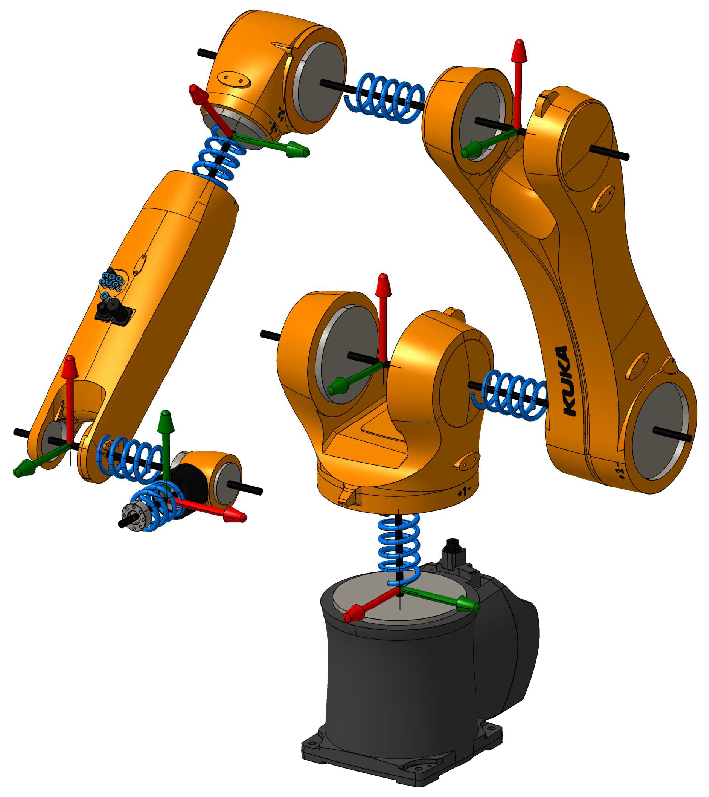
• Develop two distinct dynamic simulation models of a KUKA KR10 industrial robot in Matlab/Simscape Multibody: a 12-parameter model (12P) with only rotational joint compliance and a 24-parameter model (24P) including both rotational and effective transverse joint compliance.
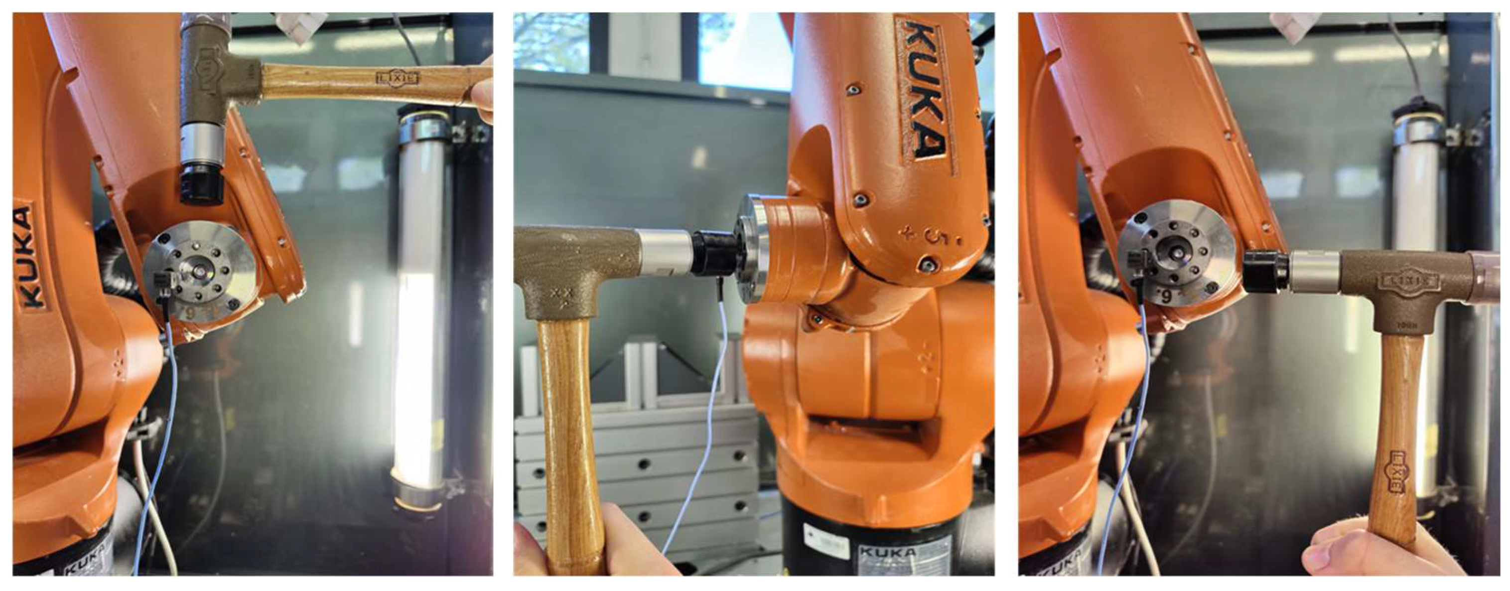
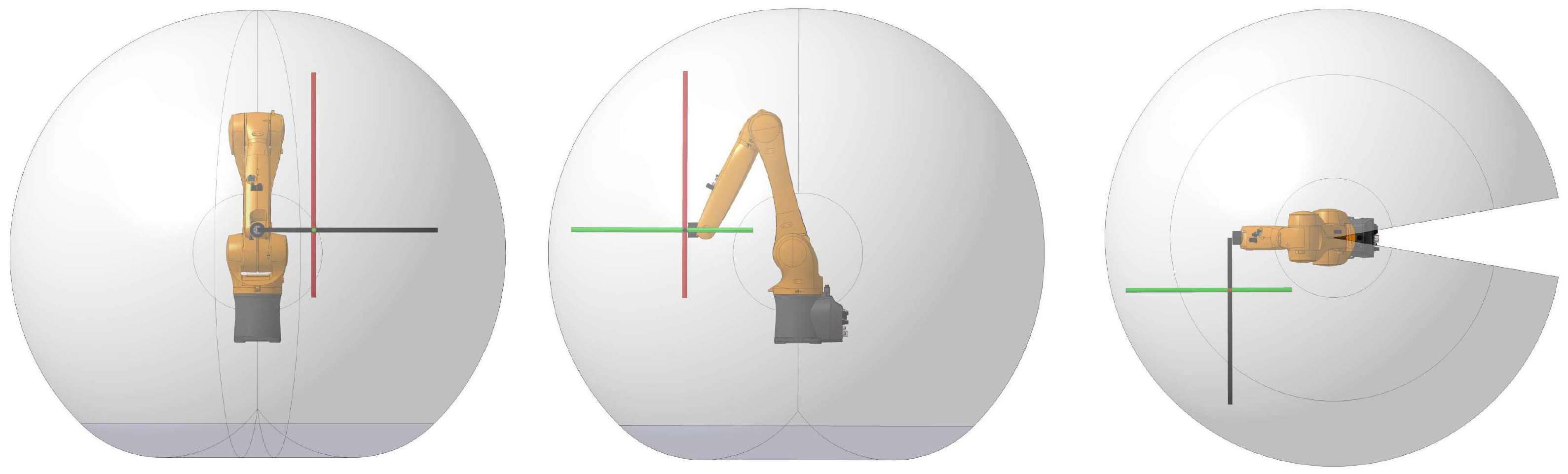
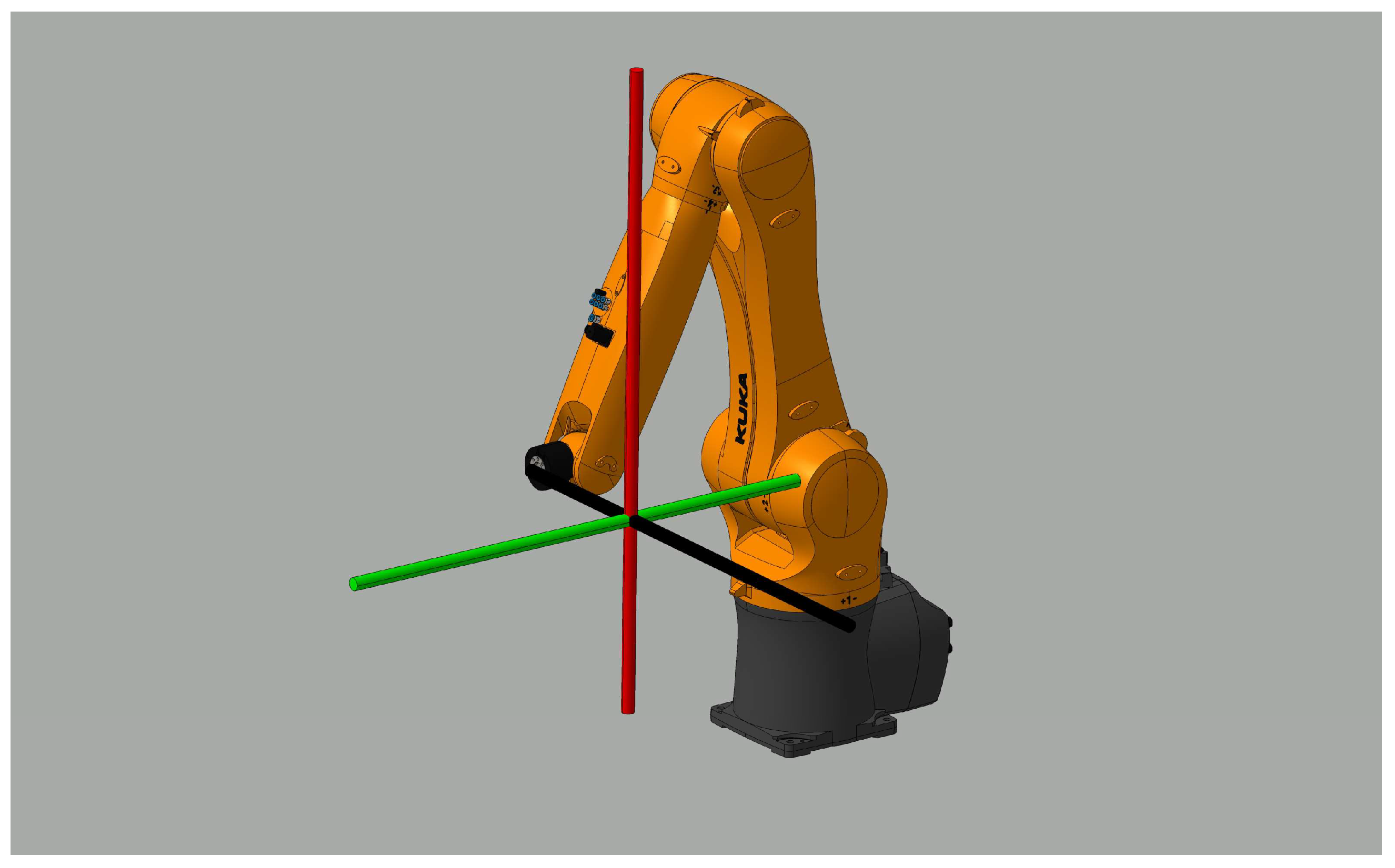
• Implement and validate a comprehensive experimental methodology using EMA (impulse hammer excitation, triaxial acceleration measurement) to acquire a rich dataset of FRFs across the robot’s workspace.
• Identify the parameters of both the 12P and 24P models using Genetic Algorithm (GA) optimization, minimizing the discrepancy between simulated and measured FRFs based on FRAC and RMSE metrics.
• Quantitatively compare the performance, accuracy, and generalizability of the identified 12P and 24P models, with a particular focus on the dynamics below 200 Hz relevant to precision manufacturing.

The main contributions of this work include (1) a detailed and validated methodology for the dynamic characterization of an industrial robot using extensive FRF measurements and Simscape modeling; (2) a quantitative comparison demonstrating the significant improvement in simulation accuracy achieved by incorporating effective transverse joint compliance (24P model) compared to a purely rotational model (12P); and (3) insights into the level of model complexity required to capture robot dynamics relevant for precision manufacturing applications up to approximately 100–200 Hz.

The remainder of this paper is structured as follows. Section 2 details the materials and methods, covering the experimental setup, the modeling approach, the GA parameter identification process, evaluation metrics, and data processing techniques. Section 3 presents the results, including the quantitative model performance comparison, Campbell diagram analysis, optimized parameters, and generalizability assessment. Section 4 discusses the interpretation of these results, methodological aspects, limitations, and practical implications. Section 5 concludes the paper, summarizing key findings and outlining directions for future research.

2. Materials and Methods

2.1. Experimental Setup

The experimental investigation focused on a KUKA KR10 R1100 sixx industrial robot. A notable feature of this robot is its use of HD gearboxes at the output shaft of each of its six joints. These drives are characterized by negligible backlash by design and possess high transmission ratios, leading to minimal backdrivability [8]. This characteristic is advantageous for static testing; when the robot brakes are engaged, the structural dynamics dominated by link inertia and joint compliance are effectively isolated from the motor-side dynamics, validating the use of static impulse hammer testing to characterize the structural system.

Dynamic excitation was applied using a PCB Piezotronics Model 086C03 modal impulse hammer equipped with an integrated force sensor. The resulting vibrations were measured using a PCB Piezotronics Model 356A45 miniature triaxial ICP accelerometer [19]. This sensor offers a sensitivity of 100 mV/g, a measurement range of ±50 g peak, and a usable frequency range from approximately 0.4 Hz to 10 kHz. The accelerometer was mounted near the robot flange (output of Axis 6) using petroleum wax (PCB P/N 080A109) [19]. Petroleum wax provides a convenient, non-permanent mounting method suitable for modal testing across multiple locations; when applied as a thin layer on clean surfaces, it offers adequate stiffness for good transmissibility within the target frequency range (up to several kHz), minimizing mass loading compared to more permanent fixtures [15,20]. Surfaces were cleaned prior to mounting to ensure good contact. Figure 1 illustrates the force application directions and the mounted sensor.

To capture pose-dependent dynamics, measurements were performed along three distinct, orthogonal paths (S1, S2, S3) within the robot’s reachable workspace, as depicted in Figure 2. Each path consisted of 40 equidistant measurement points, resulting in a total of 120 unique robot configurations. The increment between each configuration is about 1/100th of the working space (radius 1100 mm, end-to-end reach 2200 mm, increment 20 mm). This has shown to be sufficient to capture the continuously changing dynamical response of the system. At each configuration, impulse excitations were delivered sequentially in the X, Y, and Z directions relative to the sensor’s coordinate system. This comprehensive procedure yielded 360 sets of measured FRFs, providing thorough characterization of the robot’s dynamic behavior across a representative volume of its operational envelope (Figure 3).

Data acquisition was managed by an OR36 Teamwork Multianalyzer. For each measurement (excitation direction at a specific point), time data was recorded for 640 ms, including a −30 ms pre-trigger time to capture the full impulse event. An auto-trigger mechanism, based on the impulse hammer’s force signal exceeding a 7% threshold, initiated the recording. The maximum analysis frequency was set to 10 kHz, and the sampling frequency to 22.1 kHz. The frequency content effectively imparted by the impulse hammer is shown in Figure 4, indicating sufficient energy input up to approximately 800 Hz to excite the relevant structural modes.

2.2. Dynamic Modeling Approach

The KUKA KR10 robot was modeled using Matlab R2023a, leveraging the Simulink environment and the Simscape Multibody toolbox. This toolbox facilitates the creation of multi-body dynamic models based on physical network principles, employing formulations equivalent to Lagrange or Newton–Euler methods [6]. The robot’s links were modeled as rigid bodies, with mass and inertia properties derived from available CAD data, assuming standard aluminum material properties. While preliminary Finite Element Method (FEM) analysis suggested the first natural frequencies of links 2 and 4 were around 300 Hz, the rigid link assumption was deemed acceptable for this study’s primary focus on dynamics below 200 Hz. In this lower frequency range, the overall robot flexibility is typically dominated by compliance in the joints and transmission elements rather than link deformation [10].

Crucially, the dynamic models developed in Simscape were simulated directly without linearization. This approach aims to capture the inherent nonlinearities of the multi-body dynamics more accurately than methods relying on linearization around operating points [3], which can be problematic when dealing with significant configuration changes or nonlinear phenomena like friction or backlash [11,14].

Two distinct model variants were created to investigate the impact of joint model complexity:

12-Parameter Model (12P): This model represents the compliance at each of the six robot joints using a single torsional spring-damper element. This element acts purely around the primary axis of rotation for each joint (Figure 5). The model thus incorporates two parameters per joint, rotational stiffness (${\mathrm{k}}_{\mathrm{r}\mathrm{o}\mathrm{t}}$) and rotational damping (${\mathrm{d}}_{\mathrm{r}\mathrm{o}\mathrm{t}}$), resulting in a total of 12 identifiable parameters for the entire robot.

24-Parameter Model (24P): This model enhances the joint representation by adding degrees of freedom to account for effective compliance perpendicular to the primary rotation axis (Figure 6). In addition to the rotational stiffness (${\mathrm{k}}_{\mathrm{r}\mathrm{o}\mathrm{t}}$) and damping (${\mathrm{d}}_{\mathrm{r}\mathrm{o}\mathrm{t}}$), each joint model includes parameters for effective transverse stiffness (${\mathrm{k}}_{\mathrm{t}\mathrm{r}\mathrm{a}\mathrm{n}\mathrm{s}}$) and effective transverse damping (${\mathrm{d}}_{\mathrm{t}\mathrm{r}\mathrm{a}\mathrm{n}\mathrm{s}}$). These transverse parameters represent lumped compliance capturing bending or off-axis deflections within the joint/transmission structure. This approach aligns with concepts like “virtual joints” used to improve model fidelity by accounting for multi-axis flexibility [17]. It results in four parameters per joint, totaling 24 identifiable parameters. The inclusion of transverse compliance was motivated by literature suggesting its importance for accurately predicting TCP behavior [17] and the potential for complex load paths within the HD units. While true transverse behavior might involve coupled or nonlinear effects, this lumped linear parameterization provides a pragmatic way to assess the first-order impact of including these additional compliance pathways.

During simulations, the experimentally recorded time series of the impulse force (measured by the hammer) was applied as an external wrench at the Tool Center Point (TCP) of the simulated robot model. The resulting linear acceleration of the simulated TCP was computed relative to the inertial world frame. These simulated acceleration time series were then processed (identically to the experimental data) to obtain simulated FRFs for direct comparison with the measured FRFs.

2.3. Genetic Algorithm Optimization

The unknown stiffness and damping parameters for both the 12P and 24P models were identified using a Genetic Algorithm (GA), implemented via the “ga” function within Matlab’s Global Optimization Toolbox [21]. GAs are well-suited for optimizing parameters in complex, potentially non-convex problems arising from fitting nonlinear dynamic system models, where gradient-based methods might struggle with local minima [22]. Successful GA application hinges on careful setup of the algorithm’s components.

Parameter Bounds: Physically plausible lower and upper bounds were established for all stiffness and damping parameters, as detailed in

Table 1. Parameter bounds for 12P model optimization.

Axis	Parameter	Lower Bound	Upper Bound
1	${\mathrm{k}}_{\mathrm{r}\mathrm{o}\mathrm{t}}$	500 Nm/deg	5000 Nm/deg
	${\mathrm{d}}_{\mathrm{r}\mathrm{o}\mathrm{t}}$	0.0001 Nm/(deg/s)	0.7 Nm/(deg/s)
2	${\mathrm{k}}_{\mathrm{r}\mathrm{o}\mathrm{t}}$	500 Nm/deg	5000 Nm/deg
	${\mathrm{d}}_{\mathrm{r}\mathrm{o}\mathrm{t}}$	0.0001 Nm/(deg/s)	0.7 Nm/(deg/s)
3	${\mathrm{k}}_{\mathrm{r}\mathrm{o}\mathrm{t}}$	250 Nm/deg	3000 Nm/deg
	${\mathrm{d}}_{\mathrm{r}\mathrm{o}\mathrm{t}}$	0.0001 Nm/(deg/s)	0.7 Nm/(deg/s)
4	${\mathrm{k}}_{\mathrm{r}\mathrm{o}\mathrm{t}}$	100 Nm/deg	1500 Nm/deg
	${\mathrm{d}}_{\mathrm{r}\mathrm{o}\mathrm{t}}$	0.0001 Nm/(deg/s)	0.7 Nm/(deg/s)
5	${\mathrm{k}}_{\mathrm{r}\mathrm{o}\mathrm{t}}$	30 Nm/deg	1000 Nm/deg
	${\mathrm{d}}_{\mathrm{r}\mathrm{o}\mathrm{t}}$	0.0001 Nm/(deg/s)	0.7 Nm/(deg/s)
6	${\mathrm{k}}_{\mathrm{r}\mathrm{o}\mathrm{t}}$	30 Nm/deg	1000 Nm/deg
	${\mathrm{d}}_{\mathrm{r}\mathrm{o}\mathrm{t}}$	0.0001 Nm/(deg/s)	0.7 Nm/(deg/s)

(12P) and

Table 2. Parameter bounds for 24P model optimization.

Axis	Parameter	Lower Bound	Upper Bound
1	${\mathrm{k}}_{\mathrm{r}\mathrm{o}\mathrm{t}}$	500 Nm/deg	5000 Nm/deg
	${\mathrm{d}}_{\mathrm{r}\mathrm{o}\mathrm{t}}$	0.0001 Nm/(deg/s)	0.7 Nm/(deg/s)
	${\mathrm{k}}_{\mathrm{t}\mathrm{r}\mathrm{a}\mathrm{n}\mathrm{s}}$	2500 Nm/deg	80,000 Nm/deg
	${\mathrm{d}}_{\mathrm{t}\mathrm{r}\mathrm{a}\mathrm{n}\mathrm{s}}$	0.0001 Nm/(deg/s)	0.7 Nm/(deg/s)
2	${\mathrm{k}}_{\mathrm{r}\mathrm{o}\mathrm{t}}$	500 Nm/deg	5000 Nm/deg
	${\mathrm{d}}_{\mathrm{r}\mathrm{o}\mathrm{t}}$	0.0001 Nm/(deg/s)	0.7 Nm/(deg/s)
	${\mathrm{k}}_{\mathrm{t}\mathrm{r}\mathrm{a}\mathrm{n}\mathrm{s}}$	2500 Nm/deg	80,000 Nm/deg
	${\mathrm{d}}_{\mathrm{t}\mathrm{r}\mathrm{a}\mathrm{n}\mathrm{s}}$	0.0001 Nm/(deg/s)	0.7 Nm/(deg/s)
3	${\mathrm{k}}_{\mathrm{r}\mathrm{o}\mathrm{t}}$	250 Nm/deg	3000 Nm/deg
	${\mathrm{d}}_{\mathrm{r}\mathrm{o}\mathrm{t}}$	0.0001 Nm/(deg/s)	0.7 Nm/(deg/s)
	${\mathrm{k}}_{\mathrm{t}\mathrm{r}\mathrm{a}\mathrm{n}\mathrm{s}}$	1250 Nm/deg	40,000 Nm/deg
	${\mathrm{d}}_{\mathrm{t}\mathrm{r}\mathrm{a}\mathrm{n}\mathrm{s}}$	0.0001 Nm/(deg/s)	0.7 Nm/(deg/s)
4	${\mathrm{k}}_{\mathrm{r}\mathrm{o}\mathrm{t}}$	100 Nm/deg	1500 Nm/deg
	${\mathrm{d}}_{\mathrm{r}\mathrm{o}\mathrm{t}}$	0.0001 Nm/(deg/s)	0.7 Nm/(deg/s)
	${\mathrm{k}}_{\mathrm{t}\mathrm{r}\mathrm{a}\mathrm{n}\mathrm{s}}$	500 Nm/deg	5000 Nm/deg
	${\mathrm{d}}_{\mathrm{t}\mathrm{r}\mathrm{a}\mathrm{n}\mathrm{s}}$	0.0001 Nm/(deg/s)	0.7 Nm/(deg/s)
5	${\mathrm{k}}_{\mathrm{r}\mathrm{o}\mathrm{t}}$	30 Nm/deg	1000 Nm/deg
	${\mathrm{d}}_{\mathrm{r}\mathrm{o}\mathrm{t}}$	0.0001 Nm/(deg/s)	0.7 Nm/(deg/s)
	${\mathrm{k}}_{\mathrm{t}\mathrm{r}\mathrm{a}\mathrm{n}\mathrm{s}}$	150 Nm/deg	12,000 Nm/deg
	${\mathrm{d}}_{\mathrm{t}\mathrm{r}\mathrm{a}\mathrm{n}\mathrm{s}}$	0.0001 Nm/(deg/s)	0.7 Nm/(deg/s)
6	${\mathrm{k}}_{\mathrm{r}\mathrm{o}\mathrm{t}}$	30 Nm/deg	1000 Nm/deg
	${\mathrm{d}}_{\mathrm{r}\mathrm{o}\mathrm{t}}$	0.0001 Nm/(deg/s)	0.7 Nm/(deg/s)
	${\mathrm{k}}_{\mathrm{t}\mathrm{r}\mathrm{a}\mathrm{n}\mathrm{s}}$	150 Nm/deg	12,000 Nm/deg
	${\mathrm{d}}_{\mathrm{t}\mathrm{r}\mathrm{a}\mathrm{n}\mathrm{s}}$	0.0001 Nm/(deg/s)	0.7 Nm/(deg/s)

(24P). These bounds were derived from engineering estimations considering the robot’s size and structure, potential stiffness ranges for Harmonic Drives influencing ${\mathrm{k}}_{\mathrm{r}\mathrm{o}\mathrm{t}}$, and literature suggesting that transverse stiffness is typically significantly higher than rotational stiffness (${\mathrm{k}}_{\mathrm{t}\mathrm{r}\mathrm{a}\mathrm{n}\mathrm{s}}$ often being an order of magnitude larger than ${\mathrm{k}}_{\mathrm{r}\mathrm{o}\mathrm{t}}$) [23].

Initial Population Generation (“lhs_and_similarity”): A custom function generated the initial population for the GA, employing a mixed strategy to balance exploration and exploitation based on prior knowledge.

A fraction (‘ratio = 0.33’) of the individuals were created with correlated spring and damper parameters. For each such individual, a base random value was generated, and individual parameters were scaled to their respective ranges and slightly perturbed (“emphasis = 0.065”). This aimed to explore regions where joint parameters might exhibit some relationship.

The remaining individuals (“1-ratio = 0.67”) were generated using Latin Hypercube Sampling (LHS) [24]. LHS is a statistical sampling method designed to generate a near-random sample of parameter values from a multidimensional distribution, ensuring more uniform coverage of the parameter space compared to simple random sampling, which aids in global exploration.

A crucial heuristic, Damper Restriction, was applied during generation for all individuals: damping parameters (even indices in the parameter vector) were constrained to the lower 12.5% (1/8th) of their defined range. This focused the initial search towards physically realistic low damping values, which are typical for metallic structures and joints unless specific damping treatments are applied.

Fitness Function: The objective function evaluated the quality of each individual (parameter set) by comparing the simulated FRFs with the experimental FRFs from a selected subset of measurements. It aimed to minimize a cost value calculated as a weighted combination of the Root Mean Square Error (RMSE) and (1-Global FRAC) between the simulated and measured FRF matrices. A frequency-dependent weighting function (Figure 7) was applied during the FRF comparison, giving higher importance to matching the response at lower frequencies (≤200 Hz), which are often more critical for manufacturing precision.

GA Hyperparameters: Standard GA settings were used, including Stochastic Uniform Selection (“@selectionstochunif”), a Crossover Fraction of 0.85, and an Elite Count preserving approximately 4% of the best individuals (“round(0.04$·$popSize)”) in each generation. An adaptive Mutation (“@adaptiveMutation”) was implemented which dynamically adjusts the mutation rate, decreasing it linearly over generations while temporarily boosting it if the algorithm’s fitness improvement stagnates for a defined period.

Optimization Runs and Subset Selection: Various optimization runs were performed using different subsets of the experimental data (varying numbers of positions and force directions) for fitness evaluation. The final, best-performing parameter sets reported in this paper were obtained from an optimization run utilizing a representative subset comprising measurements from three positions on each of the three paths (S1, S2, S3), totaling nine measurement positions, with all three force directions included at each position (27 FRF sets used for each fitness evaluation).

12P Model Optimization: Population Size = 182, Max Generations = 32 (approx. 5800 fitness evaluations).

24P Model Optimization: Population Size = 336, Max Generations = 28 (approx. 9400 fitness evaluations).

The 24P model required roughly 1.6 times more fitness function calls due to its larger search space.

Due to the extensive computation time required for fitness evaluation with the nine-position, three-direction subset (see

Table 3. Approximate GA optimization runtimes on a 14-core CPU for different fitness evaluation subsets.

Model	One Position One Force Direction	One Position Three Force Directions	Three Positions Three Force Directions	Nine Positions Three Force Directions
12P	2 h 18 min	6 h 54 min	20 h 42 min	62 h 8 min
24P	3 h 44 min	11 h 11 min	33 h 24 min	100 h 43 min

), the final parameter refinement stage for this specific run used an objective function based only on maximizing the Global FRAC metric to expedite convergence.

Computational Effort: The optimization process is computationally intensive, as each fitness evaluation requires running a full dynamic simulation of the robot model. Parallel processing on a 14-core CPU was employed. Table 3 provides approximate runtimes for optimizing both models using different data subset sizes. The dramatic increase in runtime with the number of measurement points used for fitness evaluation highlights the practical necessity of using a carefully selected subset rather than the full dataset during optimization. The successful generalization achieved using the nine-point subset (evaluated against all 120 points, see Section 3) suggests this approach effectively balances computational feasibility and the ability to capture fundamental system dynamics.

2.4. Evaluation Metrics

The performance of the identified dynamic models was quantified by comparing the simulated FRF matrices (${\mathrm{M}}_{\mathrm{s}\mathrm{i}\mathrm{m}}$) against the experimentally measured FRF matrices (${\mathrm{M}}_{\mathrm{m}\mathrm{e}\mathrm{a}\mathrm{s}}$) using two complementary metrics. The detailed mathematical formulations are provided in Appendix B.

2.4.1. Global FRAC (Frequency Response Assurance Criterion)

Global FRAC assesses the similarity in shape between two FRF datasets [25]. It calculates the squared cosine of the corresponding FRF vectors (evaluated at each measurement position) and then averages these values. A value of 100% indicates perfect correlation (identical shape, differing only by a scaling factor), while 0% indicates no correlation. It is particularly sensitive to the correct prediction of resonance frequencies and overall FRF patterns.

2.4.2. Frobenius Similarity

This metric evaluates similarity based on the magnitude difference between the FRF matrices, utilizing the Frobenius norm [26]. It calculates the relative error between the simulated and measured matrices and expresses similarity as (1-relative error). A value of 100% indicates perfect agreement in both magnitude and phase across all frequencies and positions, while 0% indicates large discrepancies. It is sensitive to errors in predicting the amplitude of resonances and anti-resonances. Using both FRAC and Frobenius similarity provides a more comprehensive assessment than either metric alone, distinguishing between models that capture the correct dynamic modes (high FRAC) and those that also predict their amplitudes accurately (high Frobenius similarity).

2.5. Data Processing

The following steps were applied to both experimental and simulated data to obtain comparable FRFs:

• Signal Preprocessing: Raw time signals (force and acceleration) were initially processed using OROS Modal 2 software (for experimental data). Key parameters included the 640 ms signal duration and −30 ms pre-trigger time.
• FFT Calculation and Windowing: Fast Fourier Transform (FFT) was applied to convert time domain signals to the frequency domain. Standard practice for impact testing involves applying windowing functions to minimize spectral leakage caused by the finite signal duration [15]. Specifically, a force window (implicitly rectangular in this work, applied to the hammer impact signal) and an exponential window (with 25% decay over the window length, applied to the acceleration response signal) were used prior to the FFT. This combination is known to improve the quality of FRF estimates by reducing noise and leakage effects [27].
• FRF Calculation: The H1 estimator was employed to compute the FRFs (acceleration/force). The H1 estimator is commonly used in modal analysis and is known to minimize the influence of noise on the output (acceleration) measurement [15].
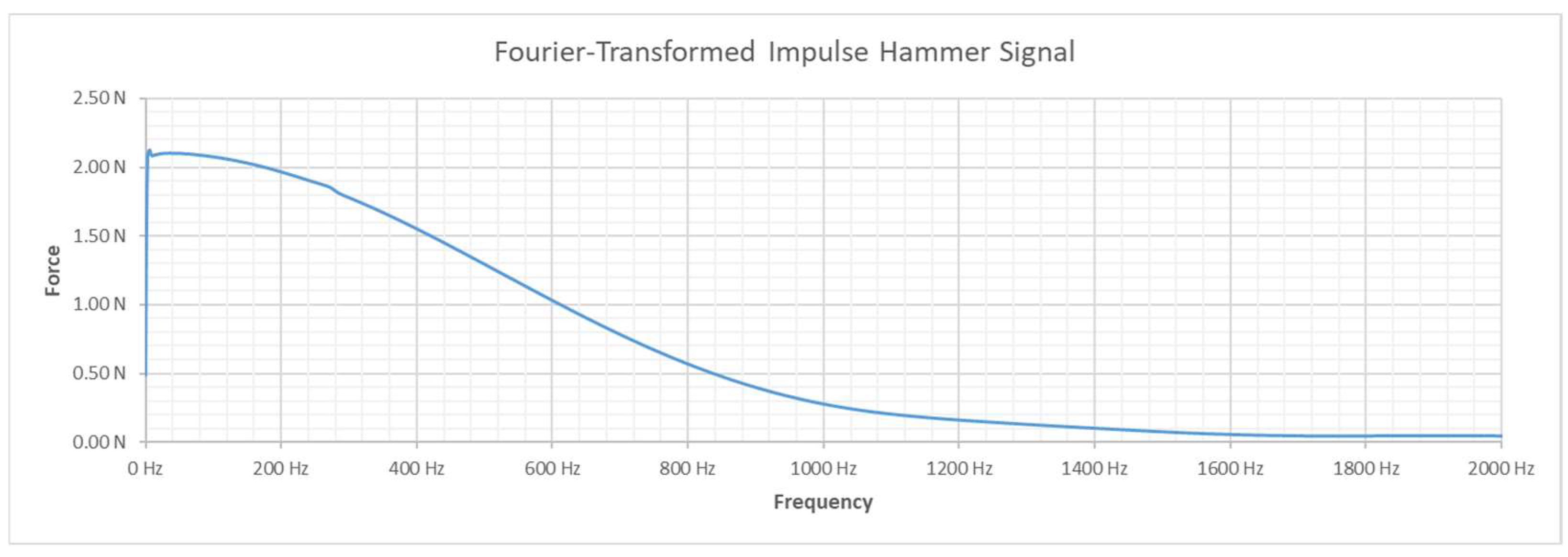
• Frequency Limitation: The analysis was conducted over two frequency ranges: the “full” range (0–800 Hz), corresponding roughly to the effective excitation bandwidth (Figure 4), and a “limited” range (0–200 Hz), selected as being most relevant to the dynamics affecting precision in typical manufacturing operations.
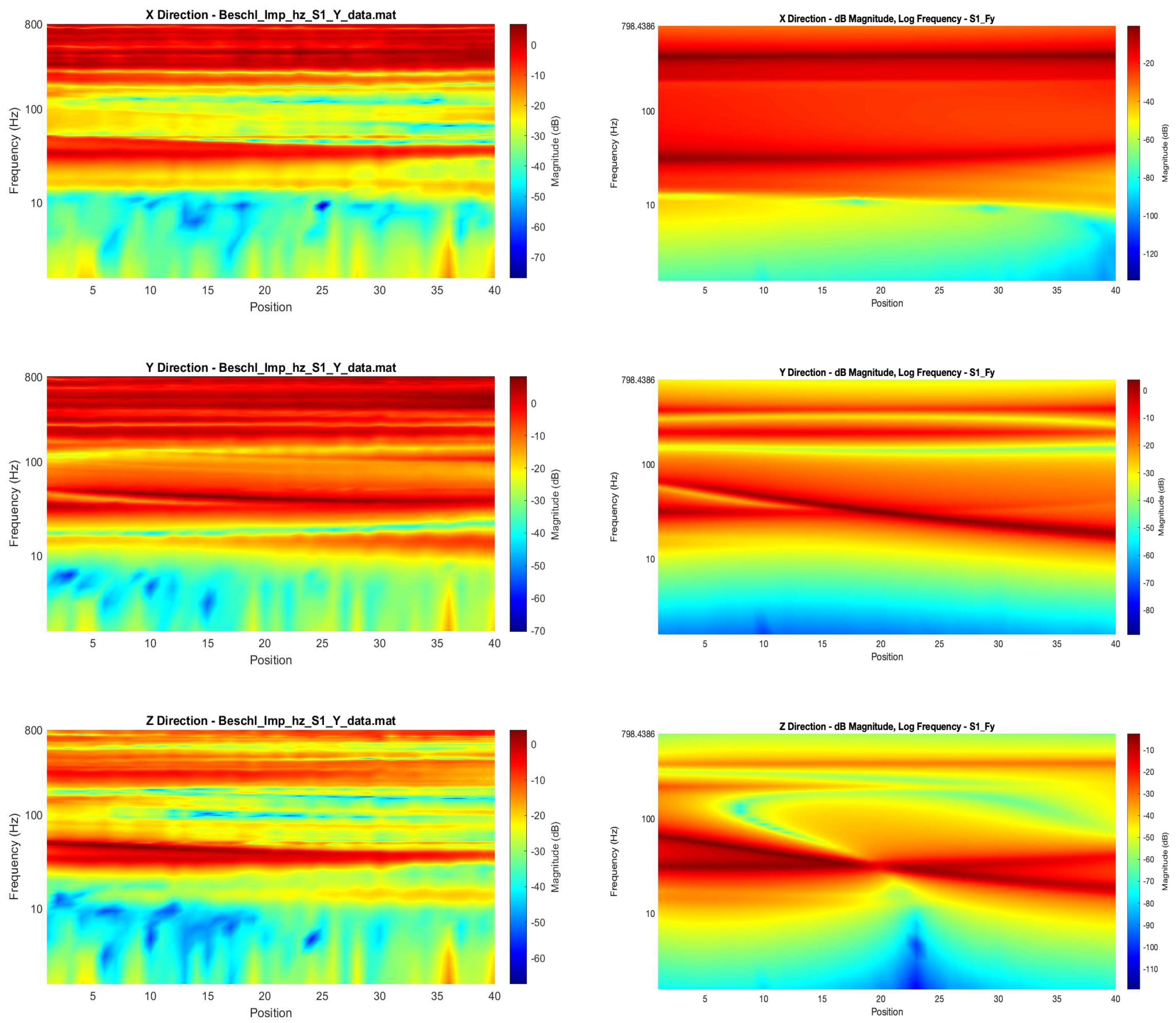
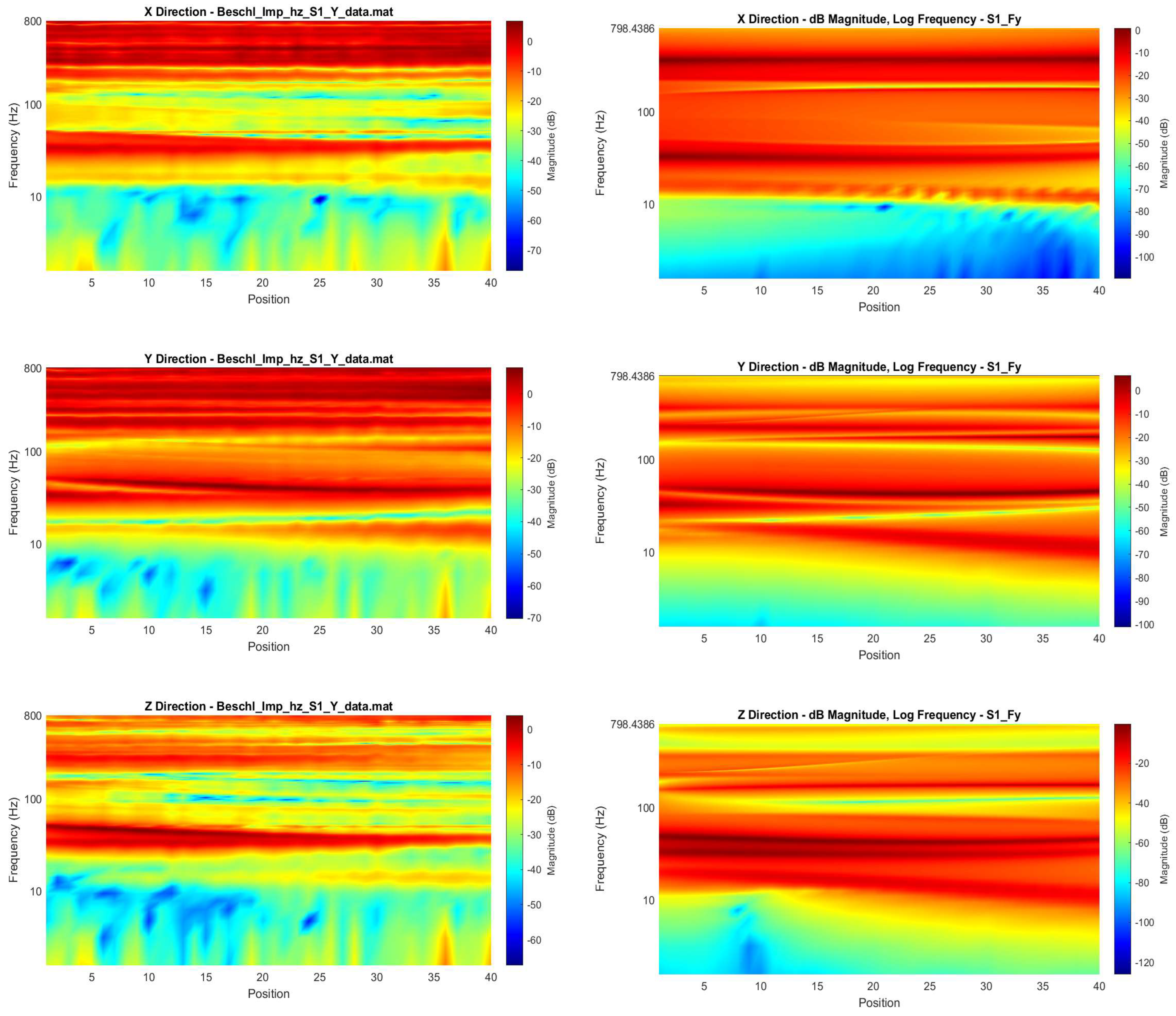
• Campbell Diagram Generation: To visualize pose-dependent dynamic behavior, FRF data was organized into Campbell diagrams [28,29]. These plots display the FRF magnitude (often in dB) as a function of frequency and measurement position along a path, providing a clear view of how resonances shift and change amplitude with robot configuration.

The consistent application of these processing steps ensures fair comparison between the experimental measurements and the simulation results.

3. Results

3.1. Model Performance

The overall performance of the 12P and 24P models, using parameters identified from the most comprehensive optimization run (nine positions across S1, S2, S3; three force directions), was evaluated across all 120 measured positions using the Global FRAC and Frobenius similarity metrics. Since measurements from nine representative positions informed the parameter estimation, these parameters were subsequently used to predict the full dynamic behavior (FRFs) at 120 distinct locations excluded from the optimization input dataset, thereby validating the model’s predictive capability on unseen data.

Table 4. Overall average performance comparison of optimized 12P and 24P models across all 120 measurement points (evaluated based on parameters identified using the nine-point S1, S2, S3 subset).

Model	Metric	Full Range (0–800 Hz)	Limited Range (≤200 Hz)
12P	Global FRAC	22.6%	40.8%
	Frobenius Similarity	5.0%	19.13%
24P	Global FRAC	36.9%	70.5%
	Frobenius Similarity	11.51%	44.9%

summarizes the average performance across the full (0–800 Hz) and limited (0–200 Hz) frequency ranges.

The results in Table 4 clearly demonstrate several key points:

• The 24P model, incorporating transverse joint compliance, significantly outperforms the 12P model across both metrics and both frequency ranges. The improvement is particularly pronounced in the limited frequency range.
• Both models achieve substantially better performance when evaluated only within the limited frequency range (≤200 Hz), indicating that the models capture the lower-frequency dynamics, most relevant for manufacturing precision, more effectively than the higher-frequency behavior.
• Global FRAC scores are consistently higher than Frobenius similarity scores for both models. This suggests that the models are generally better at predicting the shape and frequency locations of the dynamic response (captured by FRAC) than the precise amplitudes of the FRF peaks and valleys (reflected in Frobenius similarity). This discrepancy might point towards limitations in modeling damping accurately or the presence of unmodeled nonlinear amplitude-dependent effects.

Figure A1 in Appendix A provides a more detailed comparison, illustrating how performance varies depending on the data subset used for optimization and the specific path group used for evaluation. This figure shows the general trend of 24P superiority in all GA Optimization runs.

To further examine performance across different robot configurations,

Table 5. Path group performance comparison (≤200 Hz) for the final 12P and 24P models.

Model	Path Group	Global FRAC	Frobenius Similarity
12P	S1	41.8%	19.6%
	S2	46.7%	22.3%
	S3	33.9%	15.6%
24P	S1	75.0%	48.9%
	S2	70.1%	44.2%
	S3	66.2%	41.7%

presents the average performance metrics for the final identified models (optimized on the S1 + S2 + S3 subset) when evaluated separately on each of the three measurement paths (S1, S2, S3) within the limited frequency range (≤200 Hz).

Table 5 confirms that the 24P model maintains a consistent and significant performance advantage over the 12P model across all three distinct path groups, representing different regions and configurations within the robot’s workspace. While performance varies slightly between paths (e.g., both models perform slightly worse on path S3), the relative improvement offered by the 24P model remains substantial.

3.2. Campbell Diagram Analysis

Campbell diagrams are particularly effective for visualizing pose-dependent frequency response characteristics, clearly showing how resonant frequencies and amplitudes change as the robot moves along a measurement path [28].

Figure 8 and Figure 9 compare the measured and simulated Campbell diagrams for the S1 measurement path under excitation in the Y direction (${\mathrm{F}}_{\mathrm{y}}$). The plots show FRF magnitude (in dB, using log scale for frequency) versus frequency and measurement position along the path.

Several observations can be drawn from these diagrams:

• The measured data (Figure 8 and Figure 9) clearly reveals complex, pose-dependent resonance patterns. Distinct modal frequencies shift, and their amplitudes vary significantly as the robot moves along path S1. Several prominent modes are visible below 100 Hz.
• The 12P model simulation (Figure 8) captures some of the very low-frequency behavior but fails to accurately replicate the number, location, and pose-dependent shifting of most resonances observed in the measurements, particularly in the 50–200 Hz range. The predicted patterns differ substantially from the measured ones.
• The 24P model simulation (Figure 9) demonstrates significantly better agreement with the measured data. It successfully predicts the presence and approximate location of the major resonances below ~100–200 Hz. Crucially, it also captures the characteristic pose-dependency—how the frequencies and magnitudes of these resonances evolve along the path—much more accurately than the 12P model. For instance, the diagonal resonance pattern clearly visible in the measured Y direction response (Figure 8) between ~30 Hz and ~80 Hz is well-replicated by the 24P model (Figure 9).
• Above approximately 200 Hz, the agreement between the 24P simulation and the measurement deteriorates, and both models struggle to capture the complexity of the higher-frequency dynamics.

These visual comparisons strongly corroborate the quantitative findings. The Campbell diagrams provide compelling evidence that the 24P model, by including transverse compliance, captures the fundamental pose-dependent dynamic characteristics of the robot much more effectively than the 12P model, especially within the frequency range critical for many manufacturing tasks.

3.3. Optimized Parameters

The GA optimization process, using the nine-position S1/S2/S3 subset and the Global FRAC metric for final refinement, yielded the optimal parameter sets for the 12P and 24P models shown in

Table 6. Best identified parameters for the 12P model.

Axis	${\mathbf{k}}_{\mathbf{r}\mathbf{o}\mathbf{t}}$	${\mathbf{d}}_{\mathbf{r}\mathbf{o}\mathbf{t}}$
1	1962.5 Nm/deg	0.55 Nm/(deg/s)
2	765.2 Nm/deg	0.553 Nm/(deg/s)
3	789.5 Nm/deg	0.523 Nm/(deg/s)
4	577.3 Nm/deg	0.059 Nm/(deg/s)
5	232.0 Nm/deg	0.012 Nm/(deg/s)
6	268.4 Nm/deg	0.258 Nm/(deg/s)

and

Table 7. Best identified parameters for the 24P model.

Axis	${\mathbf{k}}_{\mathbf{r}\mathbf{o}\mathbf{t}}$	${\mathbf{d}}_{\mathbf{r}\mathbf{o}\mathbf{t}}$	${\mathbf{k}}_{\mathbf{t}\mathbf{r}\mathbf{a}\mathbf{n}\mathbf{s}}$	${\mathbf{d}}_{\mathbf{t}\mathbf{r}\mathbf{a}\mathbf{n}\mathbf{s}}$
1	881.7 Nm/deg	0.316 Nm/(deg/s)	5500.9 Nm/deg	0.204 Nm/(deg/s)
2	1503.8 Nm/deg	0.457 Nm/(deg/s)	22,403.9 Nm/deg	0.029 Nm/(deg/s)
3	896.7 Nm/deg	0.468 Nm/(deg/s)	10,884.6 Nm/deg	0.235 Nm/(deg/s)
4	600.8 Nm/deg	0.045 Nm/(deg/s)	10,358.5 Nm/deg	0.118 Nm/(deg/s)
5	208.8 Nm/deg	0.01 Nm/(deg/s)	6176.4 Nm/deg	0.154 Nm/(deg/s)
6	409.6 Nm/deg	0.233 Nm/(deg/s)	5528.6 Nm/deg	0.178 Nm/(deg/s)

. This subset comprised nine positions: the first (Pos 1), middle (Pos 20), and last (Pos 40) points from each of the three paths (S1, S2, S3).

Analysis of these parameter sets:

• All identified parameter values fall within the predefined bounds specified in Table 1 and Table 2, suggesting the optimization converged to a feasible solution space.
• Damping parameters (${\mathrm{d}}_{\mathrm{r}\mathrm{o}\mathrm{t}}$, ${\mathrm{d}}_{\mathrm{t}\mathrm{r}\mathrm{a}\mathrm{n}\mathrm{s}}$) tend to show relatively more variability or proximity to their bounds compared to stiffness parameters (${\mathrm{k}}_{\mathrm{r}\mathrm{o}\mathrm{t}}$, ${\mathrm{k}}_{\mathrm{t}\mathrm{r}\mathrm{a}\mathrm{n}\mathrm{s}}$). This might reflect greater difficulty in identifying damping accurately from FRF data or suggest that the simple linear viscous damping model is less representative than the linear stiffness model.
• Crucially, in the 24P model (Table 7), the identified transverse stiffness values (${\mathrm{k}}_{\mathrm{t}\mathrm{r}\mathrm{a}\mathrm{n}\mathrm{s}}$) are consistently and significantly larger than the corresponding rotational stiffness values (${\mathrm{k}}_{\mathrm{r}\mathrm{o}\mathrm{t}}$) for each joint. This aligns with physical expectations and literature suggesting that joints are typically much stiffer with respect to forces/moments perpendicular to their primary axis of rotation [23].

To highlight this last point,

Table 8. Comparison of identified stiffness ratios for the 24P model.

Axis	${\mathbf{k}}_{\mathbf{r}\mathbf{o}\mathbf{t}}$	${\mathbf{k}}_{\mathbf{t}\mathbf{r}\mathbf{a}\mathbf{n}\mathbf{s}}$	Ratio
1	881.7 Nm/deg	5500.9 Nm/deg	6.2
2	1503.8 Nm/deg	22,403.9 Nm/deg	14.9
3	896.7 Nm/deg	10,884.6 Nm/deg	12.1
4	600.8 Nm/deg	10,358.5 Nm/deg	17.2
5	208.8 Nm/deg	6176.4 Nm/deg	29.6
6	409.6 Nm/deg	5528.6 Nm/deg	13.5

calculates the ratio of identified transverse stiffness to rotational stiffness for each joint based on the 24P model parameters.

The ratios in Table 8 range from approximately 6 to 30, confirming that the optimization identified transverse stiffnesses substantially larger than rotational stiffnesses. The fact that these ratios are consistently large and vary plausibly across the different joints (e.g., higher ratios for wrist joints 4, 5, and 6, which might experience more bending loads relative to their rotational capacity) lends credibility to the physical meaningfulness of the identified 24P parameter set and validates the importance of including these transverse compliance terms.

Static payload identification on a comparable six-axis robot yielded rotational flexibility coefficients in the same range [30]. However, quasi-static methods cannot guarantee frequency domain fidelity beyond approximately 20 Hz, underscoring the advantage of the present FRF-matching strategy for dynamic behavior accuracy.

3.4. Generalizability Analysis

A key aspect of model validation is assessing a model’s ability to predict behavior under conditions not explicitly used during parameter identification. Although quantitative metrics were primarily calculated across the full dataset, qualitative assessment during the research indicated that the 24P model, optimized on the nine-point subset, maintained its predictive accuracy reasonably well when evaluated on the remaining 111 measurement points. In contrast, the 12P model’s performance degraded more significantly on points outside its optimization set. This superior generalizability of the 24P model suggests that its more comprehensive structure, particularly the inclusion of transverse compliance, allows it to capture more fundamental dynamic characteristics of the robot system, rather than simply overfitting to the specific data points used during optimization. This is further supported by the consistent performance advantage shown across different path groups in Table 5.

4. Discussion

4.1. Model Performance Interpretation

The comprehensive results presented here unequivocally demonstrate that incorporating effective transverse joint compliance, as realized in the 24-parameter (24P) model, is crucial for accurately simulating the dynamic behavior of the KUKA KR10 robot, especially for applications demanding precision below approximately 100–200 Hz. The 12-parameter (12P) model, which accounts only for compliance around the primary axis of rotation, proves fundamentally insufficient for capturing the system’s complex dynamics across its workspace.

The inadequacy of the 12P model and the success of the 24P model can be understood by considering the physical nature of robot joints and transmissions, particularly those involving Harmonic Drives. Real-world joints exhibit compliance not just in torsion, but also in bending and potentially axial directions. Neglecting these off-axis compliances, as the 12P model does, prevents the model from accurately representing how forces and motions are transmitted through the structure, especially how disturbances or excitations perpendicular to a joint’s primary axis affect TCP motion. The 24P model, by introducing lumped transverse spring-damper elements, provides the necessary degrees of freedom to approximate these effects. The significantly improved match in the Campbell diagrams (Figure 8 and Figure 9), particularly the 24P model’s ability to replicate pose-dependent evolution of resonances, visually confirms that this enhanced joint model structure leads to a more physically representative simulation. Furthermore, the identified stiffness parameters for the 24P model (Table 7), showing transverse stiffnesses significantly larger than rotational stiffnesses (Table 8), align with physical intuition and previous studies [23], bolstering confidence that the optimization found meaningful parameters representing this multi-axis compliance.

The achieved accuracy level of the 24P model in the limited frequency range (e.g., ~70% Global FRAC average, reaching ~75% on path S1) represents a substantial improvement over the 12P model and offers a level of fidelity potentially useful for practical engineering applications. While direct comparison is difficult due to varying robots, methods, and metrics, this level of agreement in FRF shape suggests the model captures the dominant modes reasonably well. Such a model can be valuable for virtual prototyping, offline programming refinement, and predicting vibration levels in precision tasks like robotic milling [5].

The diminishing accuracy above ~100–200 Hz observed for both models, even the superior 24P model, points to the limitations inherent in the chosen modeling assumptions. The primary factors likely contributing to these discrepancies are as follows:

Unmodeled Nonlinearities: Harmonic Drives are known sources of significant nonlinear behavior, including stiffness that varies with torque and position, hysteretic torque-deflection loops, and complex friction phenomena [8]. The linear spring-damper elements used in both the 12P and 24P models are simplifications that cannot fully capture these effects, which likely become more prominent at higher frequencies or under different loading conditions.

Rigid Link Assumption: While joint compliance dominates at lower frequencies [10], the flexibility of the robot links themselves becomes increasingly important as excitation frequencies approach the links’ natural frequencies (estimated at around 300 Hz for this robot). Neglecting link flexibility limits the model’s ability to predict modes involving significant link deformation.

Simplified Damping Model: The use of linear viscous damping is a common simplification. Real structural damping is often more complex, potentially exhibiting frequency-dependent or material-dependent characteristics. The observed discrepancy between higher FRAC scores (good shape matching) and lower Frobenius similarity scores (poorer amplitude matching) might partly stem from inadequacy of the linear damping model in capturing the true energy dissipation mechanisms, which strongly influence FRF peak amplitudes.

This study provides a clear illustration of the trade-off between model complexity and accuracy. The 12P model offers simplicity and lower computational cost (Table 3) but sacrifices accuracy. The 24P model introduces greater complexity and significantly increases computational demands but yields substantially better accuracy within the target frequency range (Table 4). This highlights that selecting appropriate model complexity requires careful consideration of the specific application requirements, the frequency range of interest, and the acceptable computational budget. For high-precision tasks sensitive to dynamics below 100–200 Hz, the added complexity of the 24P model appears justified by the performance gains. Achieving similar fidelity at higher frequencies would likely necessitate incorporating further complexities, such as nonlinear joint elements and flexible links.

4.2. Methodological Contributions

This work contributes through:

• Detailed Experimentation: Demonstrating a systematic and comprehensive experimental procedure for acquiring FRF data across a large portion of a robot’s workspace using standard EMA tools (impulse hammer, triaxial accelerometer). The multi-path, multi-direction measurement strategy ensures thorough dynamic characterization. The justification for specific choices, such as wax mounting [19,20] and windowing functions [27], based on established best practices [15] enhances the rigor and reproducibility of the experimental phase.
• Comparative Modeling: Quantitatively evaluating the impact of increased joint model dimensionality (12P vs. 24P) on simulation accuracy within the same Simscape Multibody framework, clearly demonstrating the substantial benefits of the higher-dimensional 24P model for this class of robot.
• Robust Parameter Identification: Showcasing the application of Genetic Algorithms for identifying parameters in complex, nonlinearizable multi-body dynamic models using frequency-domain data. The use of a tailored initial population strategy (“lhs_and_similarity”, including LHS [24] and damper restriction) and objective functions based on weighted FRF comparison metrics (FRAC, RMSE) proved effective. Notably, the successful identification and subsequent generalization achieved using only a small, representative subset of the available data (9 out of 120 positions) for optimization highlights an efficient approach to parameter identification when faced with computationally expensive simulations. This suggests that, with careful selection, a limited experimental dataset can be sufficient to capture the essential dynamics for model parameterization, mitigating the prohibitive computational cost of using the full dataset during optimization.
• Evaluation Framework: The combined use of Global FRAC [25] and Frobenius similarity [26] provides a nuanced assessment of model performance, distinguishing between accuracy in predicting resonance frequencies/shapes and accuracy in predicting response amplitudes.

4.3. Limitations

Despite the advancements, this study has several limitations that warrant acknowledgment:

• High-Frequency Accuracy: The model fidelity significantly decreases above approximately 100–200 Hz due to the simplifying assumptions made.
• Nonlinear Effects: The models employ linear spring-damper elements for joint compliance. They do not explicitly account for the known nonlinear stiffness, hysteresis, and complex friction characteristics of Harmonic Drives [31], nor potential backlash or general joint friction nonlinearities. These omissions likely contribute to discrepancies, especially under conditions involving high loads, rapid direction reversals, or very small motions where such effects are prominent.
• Rigid Links: While justified for the target frequency range, neglecting link flexibility limits accuracy at frequencies approaching or exceeding the natural frequencies of the links themselves (~300 Hz and above). Tasks involving very high accelerations or impacts might excite these modes.
• Linear Parameterization: The fundamental representation of joints using linear springs and dampers is an approximation of the likely more complex, potentially nonlinear, physical behavior.
• Computational Cost: Optimization of the 24P model remains computationally expensive (Table 3), potentially limiting the feasibility of exploring even more complex models (e.g., fully nonlinear joints or flexible links) or performing exhaustive sensitivity analyses.
• Parameter Identifiability: While GA explores the search space broadly, guaranteeing that the identified parameters represent the unique global optimum for such complex models is challenging. However, the consistency of the results (e.g., ${\mathrm{k}}_{\mathrm{t}\mathrm{r}\mathrm{a}\mathrm{n}\mathrm{s}}$, ${\mathrm{k}}_{\mathrm{r}\mathrm{o}\mathrm{t}}$) and the good generalization performance provide confidence in the identified solution.

4.4. Practical Implications:

Accurate dynamic models like the 24P variant developed here hold significant potential benefits for industrial applications:

• Improved Simulation Fidelity: More accurate models enable more reliable virtual commissioning, offline programming, and simulation-based process planning, reducing the need for costly physical trials and debugging on the actual robot.
• Enhanced Precision Task Performance: By predicting dynamic behavior (vibrations, deflections) more accurately, these models can be used to optimize trajectories, select process parameters (e.g., cutting speeds/feeds in robotic milling [5]), or design compensation strategies to improve path accuracy and surface finish in precision manufacturing tasks.
• Model-Based Control: Accurate dynamic models form the foundation for advanced model-based control algorithms aimed at actively compensating for vibrations or improving trajectory tracking performance, potentially enabling robots to perform tasks currently beyond their capabilities [7].
• Optimized Workcell Design: Simulations incorporating accurate robot dynamics can facilitate better design of robot workcells, tooling, and fixtures by predicting dynamic interactions between the robot and its environment, potentially avoiding unforeseen vibration issues.

5. Conclusions

This research undertook a comparative study of 12-parameter and 24-parameter dynamic models for a KUKA KR10 industrial robot equipped with Harmonic Drives, utilizing extensive experimental Frequency Response Function (FRF) data for parameter identification and validation. The key finding is that the 24-parameter model, which incorporates effective transverse compliance at each joint in addition to rotational compliance, demonstrates significantly superior accuracy and generalizability compared to the simpler 12-parameter model. This advantage is particularly pronounced in the frequency range below 200 Hz, which is critical for many precision manufacturing applications, where the 24P model achieved an overall average Global FRAC of 70.45% compared to 40.80% for the 12-parameter model. This result underscores the necessity of accounting for multi-axis joint compliance to achieve high-fidelity dynamic simulations of modern industrial robots.

The study successfully validated a comprehensive methodology combining thorough experimental modal analysis across the robot’s workspace with Genetic Algorithm-based parameter identification for nonlinear Simscape Multibody models. The approach proved capable of identifying physically plausible parameters for the higher-dimensional 24 parameter model, even when using a computationally feasible subset of the experimental data for optimization. While limitations remain concerning accuracy at higher frequencies (>200 Hz) and the effects of unmodeled nonlinearities (particularly from Harmonic Drives) and link flexibility, the identified 24-parameter model provides a robust and significantly improved representation of the robot’s dynamics relevant for simulation-based analysis and design of precision manufacturing tasks compared to simpler models.

Future research will focus on addressing the identified limitations to further enhance model accuracy and broaden its applicability. Promising directions include:

• Incorporating nonlinear joint models, specifically targeting the known characteristics of Harmonic Drives such as nonlinear stiffness and hysteresis, potentially using advanced system identification techniques or component-level models.
• Including link flexibility through flexible multibody dynamics (FMBD) techniques, using model order reduction methods to maintain computational tractability.
• Investigating optimized experimental designs to determine the minimum number and optimal placement of measurement points and excitation directions required to reliably identify parameters for complex models, further improving the efficiency of the characterization process.
• Employing an analytical dynamic model as a surrogate to guide parameter searches and to ensure globally optimal solutions.

References

1. Siciliano, B.; Khatib, O. (Eds.) Springer Handbook of Robotics, 2nd ed.; Springer: Berlin/Heidelberg, Germany, 2016. [Google Scholar] [CrossRef]
2. Craig, J.J. Introduction to Robotics: Mechanics and Control, 4th ed.; Pearson: London, UK, 2017; ISBN 978-0133489798. [Google Scholar]
3. Spong, M.W.; Hutchinson, S.; Vidyasagar, M. Robot Modeling and Control, 2nd ed.; Wiley: Hoboken, NJ, USA, 2020; ISBN 978-1119523994. [Google Scholar]
4. Wu, K.; Kuhlenkötter, B. Experimental Analysis of the Dynamic Stiffness in Industrial Robots. Appl. Sci. 2020, 10, 8332. [Google Scholar] [CrossRef]
5. Mejri, S.; Gagnol, V.; Le, T.P.; Sabourin, L.; Ray, P.; Paultre, P. Dynamic characterization of machining robot and stability analysis. Int. J. Adv. Manuf. Technol. 2016, 82, 351–359. [Google Scholar] [CrossRef]
6. Swevers, J.; Verdonck, W.; De Schutter, J. Dynamic Model Identification for Industrial Robots. IEEE Control. Syst. Mag. 2007, 27, 58–71. [Google Scholar] [CrossRef]
7. Albu-Schäffer, A.; Ott, C.; Hirzinger, G. A Unified Passivity-based Control Framework for Position, Torque and Impedance Control of Flexible Joint Robots. Int. J. Robot. Res. 2007, 26, 23–39. [Google Scholar] [CrossRef]
8. Harmonic Drive SE. Products. Available online: https://harmonicdrive.de/de/produkte (accessed on 15 May 2024).
9. Rhéaume, F.-E.; Champliaud, H.; Liu, Z. Understanding and modelling the torsional stiffness of harmonic drives through finite-element method. Proc. Inst. Mech. Eng. Part C J. Mech. Eng. Sci. 2009, 223, 515–524. [Google Scholar] [CrossRef]
10. Karim, A.; Hitzer, J.; Lechler, A.; Verl, A. Analysis of the dynamic behavior of a six-axis industrial robot within the entire workspace in respect of machining tasks. Int. J. Adv. Manuf. Technol. 2020, 108, 1–17. [Google Scholar] [CrossRef]
11. Wernholt, E.; Gunnarsson, S. Frequency-Domain Gray-Box Identification of Industrial Robots. In Proceedings of the 17th IFAC World Congress, Seoul, Republic of Korea, 6–11 July 2008; Volume 41, Issue 2. pp. 15–20. [Google Scholar] [CrossRef]
12. Huynh, H.N.; Verlinden, O. Direct method for updating flexible multibody systems applied to a milling robot. Robot. Comput.-Integr. Manuf. 2021, 68, 102049. [Google Scholar] [CrossRef]
13. Wu, K.; Li, J.; Zhao, H.; Zhong, Y. Review of Industrial Robot Stiffness Identification and Modelling. Appl. Sci. 2022, 12, 8719. [Google Scholar] [CrossRef]
14. Wernholt, E.; Gunnarsson, S. Nonlinear Identification of a Physically Parameterized Robot Model. In Proceedings of the 16th IFAC Symposium on System Identification, Newcastle, Australia, 29–31 March 2006; Volume 39, Issue 1. pp. 143–148. [Google Scholar] [CrossRef]
15. Ewins, D.J. Modal Testing: Theory, Practice and Application, 2nd ed.; Research Studies Press: Baldock, UK, 2000; ISBN 978-0-863-80218-8. [Google Scholar]
16. Karim, A.; Schmid, M.; Verl, A.; Hitzer, J. Autonomous modal analysis method for industrial robots based on output-only measurements. Sci. Rep. 2024, 14, 21657. [Google Scholar] [CrossRef]
17. Moberg, S.; Ohr, J.; Gunnarsson, S. A Benchmark Problem for Robust Feedback Control of a Flexible Manipulator. IEEE Trans. Control. Syst. Technol. 2009, 17, 1398–1405. [Google Scholar] [CrossRef]
18. Abele, E.; Rothenbücher, S.; Weigold, M. Cartesian Compliance Model for Industrial Robots Using Virtual Joints. Prod. Eng. Res. Dev. 2008, 2, 339–343. [Google Scholar] [CrossRef]
19. PCB Piezotronics, Inc. Model 356A45 Miniature Triaxial ICP® Accelerometer Specification Sheet. Available online: https://www.pcb.com/products?m=356a45 (accessed on 15 May 2024).
20. Avitabile, P. Modal Testing: A Practitioner’s Guide; Wiley: Hoboken, NJ, USA, 2017. [Google Scholar] [CrossRef]
21. Goldberg, D.E. Genetic Algorithms in Search, Optimization and Machine Learning; Addison-Wesley: Boston, MA, USA, 1989; ISBN 978-0-201-15767-3. [Google Scholar]
22. Deb, K. Multi-Objective Optimization Using Evolutionary Algorithms; Wiley: Chichester, UK, 2001; ISBN 978-0-471-87339-6. [Google Scholar]
23. Nubla, M.M.; Feng, L.; Menq, C.H. Joint stiffness identification of six-revolute industrial serial robots. Robot. Comput.-Integr. Manuf. 2011, 27, 947–956. [Google Scholar] [CrossRef]
24. McKay, M.D.; Beckman, R.J.; Conover, W.J. A Comparison of Three Methods for Selecting Values of Input Variables in the Analysis of Output from a Computer Code. Technometrics 1979, 21, 239–245. [Google Scholar] [CrossRef]
25. Allemang, R.J. The Modal Assurance Criterion—Twenty Years of Use and Abuse. Sound Vib. 2003, 37, 14–21. [Google Scholar]
26. Golub, G.H.; Van Loan, C.F. Matrix Computations, 4th ed.; Johns Hopkins University Press: Baltimore, MD, USA, 2013; ISBN 978-1-4214-0794-4. [Google Scholar]
27. Wang, M.Q.; Wang, Y. Unbiased expression of FRF with exponential window function in impact hammer testing. J. Sound Vib. 2004, 271, 1147–1155. [Google Scholar] [CrossRef]
28. Rao, S.S. Mechanical Vibrations, 5th ed.; Prentice Hall: Upper Saddle River, NJ, USA, 2010; ISBN 978-0-13-212819-3. [Google Scholar]
29. Berninger, T. Evaluation of an External Vibration Damping Approach for Robot Manipulators Using a Flexible Multi Body Simulation. In Proceedings of the 2019 IEEE/ASME International Conference on Advanced Intelligent Mechatronics (AIM), Hong Kong, China, 8–12 July 2019. [Google Scholar] [CrossRef]
30. Li, Y.; Gao, G.; Na, J.; Xing, Y. Error Sensitivity Flexibility Compensation of Joints for Improving the Positioning Accuracy of Industrial Robots. IEEE Trans. Autom. Sci. Eng. 2025, 22, 5335–5348. [Google Scholar] [CrossRef]
31. Zhang, H.; Ahmad, S.; Liu, G. Torque Estimation for Robotic Joint with Harmonic Drive Transmission Based on Position Measurements. IEEE Trans. Robot. 2015, 31, 322–330. [Google Scholar] [CrossRef]
Figure 1. Force application and acceleration measurement setup on the KUKA KR10 robot flange. (Left): X-direction force application; (Middle): Z-direction force application; (Right): Y-direction force application with visible triaxial accelerometer.
Actuators 14 00311 g001
Figure 2. Measurement paths shown within the robot’s working envelope (front, side, and top views).
Actuators 14 00311 g002
Figure 3. Measurement path visualization. The three orthogonal paths are shown––S1 (green), S2 (black), and S3 (red)––each containing 40 measurement points.
Actuators 14 00311 g003
Figure 4. Frequency content of the impulse hammer excitation signal (Fourier-transformed magnitude), showing energy concentrated below ~800 Hz. Measurement S2 F y , Pos 5.
Actuators 14 00311 g004
Figure 5. 12-parameter model (12P) visualization with rotational spring-damper elements (blue) at each joint. The local coordinate-frame axes are indicated by red (x-axis), green (y-axis), and black (z-axis) arrows.
Actuators 14 00311 g005
Figure 6. 24-parameter model (24P) visualization including primary rotational (blue) and effective transverse (yellow) spring-damper elements at each joint.
Actuators 14 00311 g006
Figure 7. Frequency-dependent weighting function applied in the fitness calculation, emphasizing accuracy at lower frequencies.
Actuators 14 00311 g007
Figure 8. Campbell diagram comparison. S1 F y : measured Campbell diagram. (Left), best 12 parameter model Campbell diagram; (Right), magnitude in dB [m/Ns2].
Actuators 14 00311 g008
Figure 9. Campbell diagram comparison. S1 F y : measured Campbell diagram. (Left), best 24-parameter model Campbell diagram; (Right), magnitude in dB [m/Ns2].
Actuators 14 00311 g009