Robust Time-Optimal Kinematic Control of Robotic Manipulators Based on Recurrent Neural Network Against Harmonic Noises

Abstract

Industrial and service manipulators demand implementing time-optimal kinematic control to minimize task duration in a manner of maximizing end-effector velocity during path tracking. However, achieving this objective in the presence of harmonic noise while strictly enforcing joint motion constraints remains a significant challenge. This paper introduces a novel approach that leverages dynamic recurrent neural networks (RNNs) within a constrained optimization framework to deliver robust, time-optimal kinematic control even under harmonic disturbances. We provide a thorough theoretical analysis of the RNN-based control solver, establishing its convergence and optimality. Importantly, our method maximizes end-effector speed without violating any joint velocity limits, thereby enhancing the path-tracking speed compared to previous schemes. Simulation results and physical experiments further demonstrate the effectiveness and superiority of the proposed approach.

1. Introduction

In recent decades, robotic manipulators have become ubiquitous across a wide range of industrial and service applications. Their additional degrees of freedom provide enhanced control flexibility, enabling them to execute multi-objective tasks with precision. By automating monotonous and repetitive tasks, manipulators significantly reduce the burden on human labour, allowing workers to focus on more complex responsibilities. Within the workspace, manipulators are tasked with driving their end-effectors to perform intricate and skilful operations [1]. Achieving seamless end-effector tracking requires precise kinematic control, which in turn depends on accurately managing the nonlinear relationship between joint space and workspace. However, directly solving these coupled nonlinear equations at the joint level poses significant analytical challenges [2].

Early efforts focused on achieving accurate control solutions by directly computing the pseudoinverse of the manipulator’s Jacobian matrix [3]. This approach laid the groundwork for kinematic control through the application of differential kinematics. However, relying solely on the pseudoinverse can introduce significant computational challenges, particularly when enforcing essential joint constraints for safe operation. Consequently, more advanced methodologies are necessary to enable precise kinematic control under these critical constraints.

Consequently, many approaches reformulate the problem in terms of velocity or acceleration, seeking solutions in these transformed domains. Early efforts aimed to derive control strategies by directly employing the pseudoinverse of the manipulator’s Jacobian matrix [3]. However, this method incurs significant computational burdens due to the continual need for matrix pseudoinversion over time, and it is susceptible to local instability issues [4]. In response, subsequent research reframed the control problem as a quadratic programming task [5], targeting an optimal solution while satisfying the necessary constraints. Nonetheless, since these task constraints typically involve inequalities, obtaining closed-form analytical solutions remains a challenging endeavour.

In recent years, dynamic recurrent neural networks (RNNs) have emerged as a promising tool for addressing kinematic control challenges under joint constraints. Owing to their parallel processing capabilities and suitability for analogue hardware implementation, RNN-based methods offer significant advantages over traditional serial-processing approaches [6]. These networks efficiently solve constrained optimization problems for manipulator kinematic control in noise-free environments, but they are not primarily designed for kinematic control of manipulators with time-optimality considered. For instance, Zhang et al. [7] introduced a unified joint torque optimization framework that integrates both velocity-level and acceleration-level control schemes. Similarly, Jin et al. developed an inverse-free manipulability–maximal control scheme by leveraging dynamic RNNs to optimize manipulability. Xie et al. [8] further enhanced repetitive-motion kinematic control by incorporating an orthogonal projector into an RNN model, thereby improving position-tracking precision and eliminating joint drift. Additionally, Zhang et al. [9] addressed variable joint-velocity limits using a minimum-velocity-norm optimization formulation solved by a specialized RNN, while Khan et al. [10] employed an RNN-based meta-heuristic hybrid approach for adaptive obstacle avoidance in manipulators facing arbitrarily shaped obstacles.

Although significant progress has been made in kinematic control for manipulators, most existing work primarily focuses on nominal designs without explicitly accounting for noise. In practice, RNN-based kinematic controllers encounter various types of noise during both design and implementation [11]. Several studies have addressed these challenges to develop more robust controllers [12]. While modifying the original controller to handle noise may increase design and implementation complexity, such enhancements ultimately maintain control accuracy under noisy conditions. For example, Li et al. proposed novel RNN-based control schemes that mitigate the adverse effects of harmonic and polynomial noise while preserving end-effector precision [13,14]. Tan et al. introduced an integration-enhanced, noise-tolerant method for kinematic control that guarantees finite-time convergence and improved robustness [15]. Additionally, Zhang et al. developed a kinematic controller based on a circadian rhythms neural network to prevent motion control failures caused by periodic noise [16]. Collectively, these efforts have successfully demonstrated robust kinematic control of manipulators in the presence of noise.

In a wide range of industrial applications, time efficiency is paramount for maximizing production efficiency, making the economic viability of manipulators a critical concern [17]. The core challenge arises from the limited operational speed of manipulators within their workspaces, which necessitates that end-effectors operate at peak velocity to complete tasks in the shortest possible time. This demand has driven research into the development of time-optimal kinematic control strategies. For example, Galicki investigated time-optimal control for redundant manipulators under dynamic constraints [18]. Reiter et al. introduced an efficient, higher-order kinematic control method formulated within a nonlinear programming framework [19]. Liu et al. further advanced the field by combining two linear programming problems to develop a strategy that incorporates jerk constraints [20], while Yu et al. applied a genetic algorithm with cubic uniform B-spline interpolation to optimize the time-optimal path for kinematic control [21]. Collectively, these studies demonstrate that efficient time-optimal kinematic control approaches can be successfully implemented albeit in noise-free settings to significantly enhance manipulator performance.

However, achieving time-optimal kinematic control for manipulators requires compliance with a range of internal and external constraints including physical joint angle limits, permissible joint velocity bounds, and noise disruptions. Current time-optimal control strategies often neglect these compliance issues together with noise disturbance issues in kinematic control [18,22], resulting in solutions which may not be robust enough when subjected to both joint constraints and external disturbances. Motivated by these challenges, this work focuses on developing a more robust time-optimal kinematic control strategy that effectively mitigates harmonic noise while adhering to joint constraints. To our knowledge, this is the first work to introduce a robust time-optimal kinematic control strategy using an RNN solver that simultaneously enforces joint velocity constraints and mitigates harmonic noise with a comprehensive theoretical analysis. Compared with existing RNN-based methods adopted for time-optimal kinematic control against noises, our approach offers superior time-optimal performance while reliably satisfying joint velocity limits under harmonic noise conditions.

The organization of this paper is performed as follows. Section 2 presents the problem formulation and outlines the methods for achieving time-optimal kinematic control in the presence of harmonic noise. Section 3 provides simulation and experimental results, accompanied by a detailed discussion. Finally, Section 4 concludes the paper.

2. Problem Formulation and Method

2.1. Preliminary

As previously discussed, this paper aims to introduce a robust time-optimal kinematic control strategy for manipulators operating in environments with harmonic noise. Before detailing the proposed method, we first present the problem formulation concerning time-optimal kinematic control under harmonic noise.

In robotic manipulator motion planning and kinematic control, end-effectors are required to complete path-tracking tasks within a specified time T. Given the same desired end-effector path trajectory $r_d$, it is usually expected to achieve a fast speed to make the allocated task time minimal, i.e.,

$$t_{\mathrm{task}}=\min T=G\left(r_d\right)$$

(1)

where $G(·)$ represents a nonlinear mapping function that relates the desired trajectory $r_d$ to the optimal task time. Time-optimal kinematic control under constraints is focusing on designing control inputs that drive a manipulator from an initial state to a desired final state in the minimum possible time. It involves maximizing the system’s actuation limits while adhering to constraints. The goal is to achieve the fastest feasible trajectory without violating physical or operational limits. One conventional time-optimal (kinematic) control strategy is the “Bang-Bang” control, which uses maximum control effort for most of the trajectory, but it switches abruptly between extremes and makes states s often lie at the constraint boundaries. Another representative time-optimal (kinematic) control method is pre-computing time-optimal paths using a system’s dynamic or kinematic equations, assuming perfect prior knowledge of system parameters and ignores disturbances.

Generally, during the solution process of kinematic control, harmonic noises are frequently appearing, which may degrade the kinematic control efficiency and end-effector tracking performance. For example, harmonic noises can corrupt sensor and control signals, leading to erroneous position or velocity measurements and causing unintended actuator movements. Kinematic controllers, which assume idealized motion, cannot account for these dynamic disturbances, leading to unmoderated deviations. Throughout this work, only the harmonic type noise is considered for its interference to the corresponding time-optimal kinematic controller via theoretical, simulation and experimental validation, and other types of noises are not introduced for further investigation. In this situation, the time optimality relation may be corrupted as well since the solution of kinematic control is polluted as $\tilde{G}\left(r_d\right)$, i.e., the actual task time becomes

$$t_{\mathrm{task}}^{\prime }=\min \tilde{T}=\tilde{G}\left(r_d\right)$$

(2)

Minimizing the allocated task time for an end-effector to achieve time-optimal kinematic control presents several challenges. Maximizing joint velocities to reduce task duration can lead to violations of motion constraints, such as exceeding joint velocity limits. While the goal is for the end-effector to follow the desired trajectory at the specified speed, attempts to accelerate the task may result in surpassing these constraints. Therefore, it is crucial to balance the need for speed with adherence to the manipulator’s physical limitations. To further promote the current time-optimality and reduce the allocated task time more, increasing the joint velocity and as a result, accelerate the end-effector’s motion is essential, so holding the restriction of joint velocity limits should not be compulsory.

2.2. Time-Optimal Kinematic Controller Without Perturbed Noise

To design a time-optimal kinematic control for the manipulator’s end-effector tracking task without noise considered, the time-optimal kinematic controller should follow the following optimization paradigm [17]:

$$\begin{array}{c}\hfill \max k\parallel {\dot{r}}_d{\parallel }^2\end{array}$$

(3)

where the tuning variable $k>0$ is used to maximize the speed of the end-effector under the desired end-effector velocity ${\dot{r}}_d$. Although the velocity/speed of the end-effector can be maximized, the manipulator has to satisfy physical and safety constraints in the joint space, the following optimization framework is thus proposed equivalently:

$$\begin{array}{c}\hfill \begin{array}{cc}& \underset{k}{\min }-k{\parallel {\dot{r}}_d\parallel }^2\hfill \\ & \mathrm{s}.\mathrm{t}.\left\{\begin{array}{c}{\dot{\theta }}^{-}\le \dot{\theta }\le {\dot{\theta }}^{+}\hfill \\ \dot{r}-k{\dot{r}}_d=0\hfill \end{array}\right.\hfill \end{array}\end{array}$$

(4)

where ${\dot{\theta }}^{-}$ and ${\dot{\theta }}^{+}$ are, respectively, the lower and upper bounds for the joint velocity variable $\dot{\theta }$. For now, the optimization problem above can be solved by determining the optimal variable k under these constraints.

According to [17], optimization problem (4) can be further reformulated as the following paradigm:

$$\begin{array}{c}\hfill \begin{array}{cc}& \underset{\omega }{\min }{\omega }^T{{\rm Y}}^T{\rm Y}\omega /2-{\chi }^T\omega \hfill \\ & \mathrm{s}.\mathrm{t}.\left\{\begin{array}{c}\omega \in \Omega \hfill \\ {\rm Y}\omega =0\hfill \end{array}\right.\hfill \end{array}\end{array}$$

(5)

where $\omega ={[{\dot{\theta }}^T,k^T]}^T$, $\Omega =\{\omega \in R^{n+1}|{\dot{\theta }}^{-}\le \dot{\theta }\le {\dot{\theta }}^{+},k\ge 0\}$, $\chi =[0_n^T,1]$, and ${\rm Y}=[J,-{\dot{r}}_d]$

To obtain the time-optimal kinematic controller from the optimization paradigm (5) based on RNN, firstly we need to define the following Lagrangian function:

$$L(\omega ,\lambda )={\omega }^T{{\rm Y}}^T{\rm Y}\omega /2-{\chi }^T\omega +{\lambda }^T{\rm Y}\omega$$

(6)

where $\lambda$ denotes the Lagrangian multiplier vector. Finding the partial derivatives of it with respect to $\omega$ and $\lambda$, it will export:

$$\left\{\begin{array}{c}{\displaystyle \frac{\partial L}{\partial \omega }}={\rm Y}\omega -\chi +{{\rm Y}}^T\lambda \hfill \\ {\displaystyle \frac{\partial L}{\partial \lambda }}={\rm Y}\omega \hfill \end{array}\right.$$

(7)

Drawing from the design principles of the primal-dual neural network, we formulate the ensuing dynamic state equations as follows:

$$\left\{\begin{array}{c}ϵ\dot{\omega }=-\omega +P_{\Omega }(\omega -{\displaystyle \frac{\partial L\left(\omega \right)}{\partial \omega }})\hfill \\ ϵ\dot{\lambda }={\rm Y}\omega \hfill \end{array}\right.$$

(8)

and its detailed and expanded form is as follows:

$$\left\{\begin{array}{c}ϵ\dot{\omega }=-\omega +P_{\Omega }(\omega -{\rm Y}\omega +\chi -{{\rm Y}}^T\lambda )\hfill \\ ϵ\dot{\lambda }={\rm Y}\omega \hfill \end{array}\right.$$

(9)

where $P_{\Omega }(·)$ denotes a piecewise projection function array, and $ϵ>0$ is a parameter which scales the convergence of the time-optimal kinematic controller (9). On its effect for the kinematic control performance, refer to [17] for details.

On optimality and convergence properties of the time-optimal kinematic controller (9) in a noise-free manner, we have the following theoretical results.

Theorem 1.

For time-optimal kinematic controller (9) without noise perturbed for a manipulator, it is equivalent to the optimal solution of the time-optimal optimization paradigm (5) which guarantees maximization of end-effector velocity.

Proof. 

The detailed proof can summarized and extended according to [17].    □

After proving optimality, we proceed to investigate the convergence of the time-optimal kinematic controller (9) without noise disturbance. Before analyzing convergence properties, we introduce a useful lemma.

Theorem 2.

On time-optimal kinematic controller (9) without noise disturbed for a manipulator, it is stable to make its state variable globally converge to the optimal solution of time-optimal optimization paradigm (5).

Proof. 

The detailed proof can summarized and extended according to [17] as well.    □

2.3. Time-Optimal Kinematic Controller Under Harmonic Noise

The time-optimal kinematic controller (9) based on RNN is depicted in a noise-free situation. The resultant time-optimal kinematic controller can be obtained when the state equilibrium point of (9) is achieved by letting $\dot{\omega }=0$ and $\dot{\lambda }=0$. In practice, noises inevitably disturb the time-optimal kinematic controller and should be considered in its modelling. When harmonic noises are exerted on such a kinematic controller, we have the following perturbed time-optimal kinematic controller model:

$$\left\{\begin{array}{c}ϵ\dot{\widehat{\omega }}=-\omega +P_{\Omega }(\omega -{\rm Y}\omega +\chi -{{\rm Y}}^T\lambda )+\widehat{\varphi }\hfill \\ ϵ\dot{\lambda }={\rm Y}\omega \hfill \end{array}\right.$$

(10)

where $\widehat{\varphi }$ denotes a disturbance variable to the kinematic controller, which results from the harmonic noise $\varphi$. The specific form of such a disturbance variable $\widehat{\varphi }$ is initially unknown. When the harmonic noise is additively exerted, the dynamic process of variable $\omega$ is thus perturbed in the original time-optimal kinematic controller.

Specifically, the involved harmonic noise $\varphi$ is defined as follows. The harmonic noise $\varphi$ with frequencies $f_i,i\in \{1,2,\cdots ,l\}$ is $\varphi ={\sum }_{i=1}^l{\varphi }_i+{\varphi }_0$ where ${\varphi }_0$ is a constant bias and ${\varphi }_i=A_i\sin (2\pi f_{i}t+{\psi }_i)$ with ${\psi }_i$ and $A_i$ being the unknown phase and the unknown amplitude for the $f_i$-frequency noise. Such a harmonic noise involve a noise dynamics relation ${\ddot{\varphi }}_i=-4{\pi }^2{f}_i^2{\varphi }_i$. The parameters (including frequencies) of the harmonic noise are not necessarily known prior to the design of the ensuing time-optimal kinematic controller, and the resultant disturbance variable $\widehat{\varphi }$ from the harmonic noise $\varphi$ appears with its parameters randomly configured. Therefore the time-optimal kinematic controller under such type of harmonic noise becomes:

$$\left\{\begin{array}{c}ϵ\dot{\widehat{\omega }}=-\omega +P_{\Omega }(\omega -{\rm Y}\omega +\chi -{{\rm Y}}^T\lambda )+\widehat{\varphi }\hfill \\ ϵ\dot{\lambda }={\rm Y}\omega \hfill \\ \widehat{\varphi }=-c_0ϵ\omega -c_0{\mu }_0-ϵ\sum _{i=1}^l{\mu }_i\hfill \\ {\dot{\mu }}_0=\omega -P_{\Omega }(\omega -{\rm Y}\omega +\chi -{{\rm Y}}^T\lambda )\hfill \\ {\dot{\mu }}_i={\eta }_i+c_1(ϵ\omega +{\mu }_0)\hfill \\ {\dot{\eta }}_i=-4{\pi }^2{f}_i^2{\mu }_i\hfill \end{array}\right.$$

(11)

where ${\mu }_0$ denotes the residual dynamics state of the time-optimal kinematic controller, ${\mu }_i$ and ${\eta }_i$ denote the ith intermediate state variables which describe dynamics of the harmonic noise with noise violation measure ${\mu }_0$, $ϵ>0$, $c_0>0$ and $c_1>0$ denote the intermediate coefficients which associate the harmonic-noise-induced disturbance and the time-optimal kinematic controller. The pseudo-code diagram of implementing the RNN framework for time-optimal kinematic control against harmonic noises is illustrated by Algorithm 1.

Algorithm 1 The Dynamic RNN Framework to Implement the Time-Optimal Kinematic Controller Under Harmonic Noise

Require: Input: desired path $r_d$, Jacobian matrix J, the maximum allocated time $T_{max}$, noise frequency $f_i,(i=\{1,2,\cdots ,l\})$, noise amplitude $A_i$, noise phase ${\psi }_i$ Ensure: Output: resolved joint angle $\theta$ and joint velocity $\dot{\theta }$   Initialize hidden state $\theta \left(0\right)$, $k\left(0\right)$, $\dot{\theta }\left(0\right)$   for $t=1$ to $T_{max}$ do      if $t\le T_{max}$ then        Update the state variables of (10) {Dynamics updating via ODE-sovler (10)}      else        Break {Early termination for overtime operations}      end if      Obtain joint angle $\theta$ {Return time series}   end for   return the acutual path $r\leftarrow J\theta$ {Return time series}

As to the convergence and optimality of time-optimal kinematic controller (11) against harmonic noises, here are the following theoretical results.

Theorem 3.

For time-optimal kinematic controller (11) disturbed by the harmonic noise in the form of $\varphi ={\sum }_{i=1}^l{\varphi }_i$ where ${\varphi }_0$ is a constant and ${\varphi }_i=A_i\sin (2\pi f_{i}t+{\psi }_i)$ with ${\psi }_i$ and $A_i$ being the unknown initial phase and the unknown amplitude for the $f_i$-frequency noise with frequencies $f_i,i\in \{1,2,\cdots ,l\}$, time-optimal kinematic controller (11) is able to stabilize the manipulator to solve for optimal solution of (5).

Proof. 

Firstly, let us define the distance variable as follows:

$$\xi =-P_{\Omega }(\omega -{\rm Y}\omega +\chi -{{\rm Y}}^T\lambda )+\omega$$

□

In this case, the time-optimal kinematic controller (11) against noise becomes

$$\left\{\begin{array}{c}ϵ\dot{\widehat{\omega }}=-\xi +\widehat{\varphi }\hfill \\ ϵ\dot{\lambda }={\rm Y}\omega \hfill \\ \widehat{\varphi }=-c_0ϵ\omega -c_0{\mu }_0-ϵ\sum _{i=1}^l{\mu }_i\hfill \\ {\dot{\mu }}_0=\xi \hfill \\ {\dot{\mu }}_i={\eta }_i+c_1(ϵ\omega +{\mu }_0)\hfill \\ {\dot{\eta }}_i=-4{\pi }^2{f}_i^2{\mu }_i\hfill \end{array}\right.$$

(12)

As $\dot{\omega }=\dot{\widehat{\omega }}+{\varphi }_0+{\sum }_{i=1}^l{\varphi }_i$ holds, considering (12), we further have

$$\begin{array}{cc}\hfill ϵ\dot{\omega }+\xi =& ϵ\dot{\widehat{\omega }}+ϵ{\varphi }_0+ϵ\sum _{i=1}^l{\varphi }_i\hfill \\ \hfill =& -c_0ϵ\omega -c_0{\mu }_0-ϵ\sum _{i=1}^l{\mu }_i+ϵ{\varphi }_0+ϵ\sum _{i=1}^l{\varphi }_i\hfill \\ \hfill =& -c_0(ϵ\omega +{\mu }_0-ϵ{\varphi }_0/c_0)-ϵ\sum _{i=1}^l({\mu }_i-{\varphi }_i)\hfill \end{array}$$

(13)

Since ${\dot{\mu }}_0=\xi$ and ${\dot{\varphi }}_0=0$, next we can derive

$${\displaystyle \frac{d(ϵ\omega +{\mu }_0-ϵ{\varphi }_0/c_0)}{dt}}=ϵ\dot{\omega }+{\dot{\mu }}_0-ϵ{\dot{\varphi }}_0/c_0=ϵ\dot{\omega }+\xi$$

(14)

which yields

$${\displaystyle \frac{d(ϵ\omega +{\mu }_0-ϵ{\varphi }_0/c_0)}{dt}}=-c_0(ϵ\omega +{\mu }_0-ϵ{\varphi }_0/c_0)-ϵ\sum _{i=1}^l({\mu }_i-{\varphi }_i)$$

(15)

According to the dynamics of ${\mu }_i$, we further obtain

$$\begin{array}{cc}\hfill {\displaystyle \frac{d({\mu }_i-{\varphi }_i)}{dt}}& ={\eta }_i-{\dot{\varphi }}_i+c_1(ϵ\omega +{\mu }_0)\hfill \\ \hfill & ={\eta }_i-{\dot{\varphi }}_i+ϵc_1{\varphi }_0/c_0+c_1(ϵ\omega +{\mu }_0-ϵ{\varphi }_0/c_0)\hfill \end{array}$$

(16)

Since ${\dot{\varphi }}_0=0$ and ${\ddot{\varphi }}_i=-4{\pi }^2{f}_i^2\sin (2\pi f_{i}t+{\psi }_i)=-4{\pi }^2{f}_i^2{\varphi }_i$, we have extra expressions as

$${\displaystyle \frac{d({\eta }_i-{\dot{\varphi }}_i+ϵc_1{\varphi }_0/c_0)}{dt}}=-4{\pi }^2{f}_i^2({\mu }_i-{\varphi }_i)$$

(17)

and

$${\displaystyle \frac{d({\mu }_i-{\varphi }_i)}{dt}}=c_1(ϵ\omega +{\mu }_0-ϵ{\varphi }_0/c_0)+{\eta }_i-{\dot{\varphi }}_i+c_1ϵ{\varphi }_0/c_0$$

(18)

To further investigate the stability and convergence of time-optimal kinematic controller (11) against harmonic noise, let us define a Lyapunov function as follows:

$$\begin{array}{cc}\hfill V& ={\displaystyle \frac{1}{2ϵ}}{(ϵ\omega +{\mu }_0-ϵ{\varphi }_0/c_0)}^T(ϵ\omega +{\mu }_0-ϵ{\varphi }_0/c_0)+\hfill \\ \hfill & {\displaystyle \frac{1}{8c_1{\pi }^2{f}_i^2}}{({\eta }_i-{\dot{\varphi }}_i+ϵc_1{\varphi }_0/c_0)}^T({\eta }_i-{\dot{\varphi }}_i+ϵc_1{\varphi }_0/c_0)+\hfill \\ \hfill & \sum _{i=1}^l{\displaystyle \frac{1}{2c_1}}{({\mu }_i-{\varphi }_i)}^T({\mu }_i-{\varphi }_i)\ge 0\hfill \end{array}$$

(19)

The time derivative of the Lyapunov function is

$$\begin{array}{cc}\hfill \dot{V}& ={\displaystyle \frac{1}{ϵ}}{(ϵ\omega +{\mu }_0-ϵ{\varphi }_0/c_0)}^T{\displaystyle \frac{d(ϵ\omega +{\mu }_0-ϵ{\varphi }_0/c_0)}{dt}}+\hfill \\ \hfill & \sum _{i=1}^l{\displaystyle \frac{1}{4c_1{\pi }^2{f}_i^2}}{({\eta }_i-{\dot{\varphi }}_i+ϵc_1{\varphi }_0/c_0)}^T{\displaystyle \frac{d({\eta }_i-{\dot{\varphi }}_i+ϵc_1{\varphi }_0/c_0)}{dt}}\hfill \\ \hfill & +\sum _{i=1}^l{\displaystyle \frac{1}{c_1}}{({\mu }_i-{\varphi }_i)}^T{\displaystyle \frac{d({\mu }_i-{\varphi }_i)}{dt}}\hfill \\ \hfill & ={\displaystyle \frac{1}{ϵ}}{(ϵ\omega +{\mu }_0-ϵ{\varphi }_0/c_0)}^T[-c_0(ϵ\omega +{\mu }_0-ϵ{\varphi }_0/c_0)-ϵ\sum _{i=1}^l({\mu }_i-{\varphi }_i)]\hfill \\ \hfill & +\sum _{i=1}^l{\displaystyle \frac{1}{4c_1{\pi }^2{f}_i^2}}{({\eta }_i-{\dot{\varphi }}_i+ϵc_1{\varphi }_0/c_0)}^T[-4{\pi }^2{f}_i^2({\mu }_i-{\varphi }_i)]\hfill \\ \hfill & +\sum _{i=1}^l{\displaystyle \frac{1}{c_1}}{({\mu }_i-{\varphi }_i)}^T[c_1(ϵ\omega +{\mu }_0-ϵ{\varphi }_0/c_0)+{\eta }_i-{\dot{\varphi }}_i+c_1ϵ{\varphi }_0/c_0]\hfill \\ \hfill & =-{\displaystyle \frac{c_0}{ϵ}}{(ϵ\omega +{\mu }_0-ϵ{\varphi }_0/c_0)}^T(ϵ\omega +{\mu }_0-ϵ{\varphi }_0/c_0)-{(ϵ\omega +{\mu }_0-ϵ{\varphi }_0/c_0)}^T\sum _{i=1}^l({\mu }_i-{\varphi }_i)\hfill \\ \hfill & -\sum _{i=1}^l{\displaystyle \frac{1}{c_1}}{({\eta }_i-{\dot{\varphi }}_i+ϵc_1{\varphi }_0/c_0)}^T({\mu }_i-{\varphi }_i)+\sum _{i=1}^l{({\mu }_i-{\varphi }_i)}^T(ϵ\omega +{\mu }_0-ϵ{\varphi }_0/c_0)\hfill \\ \hfill & +\sum _{i=1}^l{\displaystyle \frac{1}{c_1}}{({\mu }_i-{\varphi }_i)}^T({\eta }_i-{\dot{\varphi }}_i+c_1ϵ{\varphi }_0/c_0)\hfill \end{array}$$

(20)

Because

$${(ϵ\omega +{\mu }_0-ϵ{\varphi }_0/c_0)}^T\sum _{i=1}^l({\mu }_i-{\varphi }_i)=\sum _{i=1}^l{({\mu }_i-{\varphi }_i)}^T(ϵ\omega +{\mu }_0-ϵ{\varphi }_0/c_0)$$

and

$$\sum _{i=1}^l{\displaystyle \frac{1}{c_1}}{({\eta }_i-{\dot{\varphi }}_i+ϵc_1{\varphi }_0/c_0)}^T({\mu }_i-{\varphi }_i)=\sum _{i=1}^l{\displaystyle \frac{1}{c_1}}{({\mu }_i-{\varphi }_i)}^T({\eta }_i-{\dot{\varphi }}_i+c_1ϵ{\varphi }_0/c_0)$$

always hold, the time derivative $\dot{V}$ depicted by (20) can be further simplified as

$$\dot{V}=-{\displaystyle \frac{c_0}{ϵ}}{(ϵ\omega +{\mu }_0-ϵ{\varphi }_0/c_0)}^T(ϵ\omega +{\mu }_0-ϵ{\varphi }_0/c_0)\le 0$$

(21)

which indicates that time-optimal kinematic controller (11) against harmonic noise is stable. When $\dot{V}=0$, we can evidently see that

$${\displaystyle \frac{c_0}{ϵ}}{(ϵ\omega +{\mu }_0-ϵ{\varphi }_0/c_0)}^T(ϵ\omega +{\mu }_0-ϵ{\varphi }_0/c_0)=0$$

(22)

According to the well-known LaSalle’s invariance theorem, we can obtain

$$\underset{t\to +\infty }{\lim }ϵ\omega +{\mu }_0-ϵ{\varphi }_0/c_0=0$$

(23)

Its first-order and second-order time derivatives are, respectively,

$$ϵ\dot{\omega }+{\dot{\mu }}_0-ϵ{\dot{\varphi }}_0/c_0=-c_0(ϵ\omega +{\mu }_0-ϵ{\varphi }_0/c_0)-ϵ\sum _{i=1}^l({\mu }_i-{\varphi }_i)$$

(24)

and

$$\begin{array}{cc}\hfill & c_0^2(ϵ\omega +{\mu }_0-ϵ{\varphi }_0/c_0)+c_0ϵ\sum _{i=1}^l({\mu }_i-{\varphi }_i)\hfill \\ \hfill & -ϵ\sum _{i=1}^l[{\eta }_i-{\dot{\varphi }}_i+ϵc_1{\varphi }_0/c_0+c_1(ϵ\omega +{\mu }_0-ϵ{\varphi }_0{c}_0)]\hfill \end{array}$$

(25)

which are bounded. According to Barbalat’s lemma, we have

$$\underset{t\to +\infty }{\lim }ϵ\dot{\omega }+{\dot{\mu }}_0-ϵ{\dot{\varphi }}_0/c_0=\underset{t\to +\infty }{\lim }-c_0(ϵ\omega +{\mu }_0-ϵ{\varphi }_0/c_0)-ϵ\sum _{i=1}^l({\mu }_i-{\varphi }_i)=0$$

(26)

Additionally, as $\widehat{\varphi }=-c_0ϵ\omega -c_0{\mu }_0-ϵ{\sum }_{i=1}^l{\mu }_i$, thus we can obtain

$$\underset{t\to +\infty }{\lim }\widehat{\varphi }=\underset{t\to +\infty }{\lim }-ϵ{\varphi }_0-ϵ\sum _{i=1}^l{\varphi }_i=-ϵ\underset{t\to +\infty }{\lim }\varphi$$

(27)

which indicates that the disturbance variable $\widehat{\varphi }$ is of the form of harmonic noise $\varphi$ to the controller, and the $ϵ$ can be regarded as an amplifier factor of the harmonic noises.

Recall that $\xi ={\dot{\mu }}_0$ and ${\dot{\varphi }}_0=0$, it can be derived that

$$ϵ\dot{\omega }+{\dot{\mu }}_0-ϵ{\dot{\varphi }}_0/c_0=ϵ\dot{\omega }+\xi$$

(28)

So we obtain

$$\underset{t\to +\infty }{\lim }ϵ\dot{\omega }+{\dot{\mu }}_0-ϵ{\dot{\varphi }}_0/c_0=\underset{t\to +\infty }{\lim }ϵ\dot{\omega }+\xi =0$$

(29)

According to the first equation of the time-optimal kinematic controller (9) that is associated with $\omega$ and the definition $\xi =-P_{\Omega }(\omega -{\rm Y}\omega +\chi -{{\rm Y}}^T\lambda )+\omega$ in the very beginning of the proof, we evidently then obtain

$$\underset{t\to +\infty }{\lim }ϵ\dot{\omega }=\underset{t\to +\infty }{\lim }-\omega +P_{\Omega }(\omega -{\rm Y}\omega +\chi -{{\rm Y}}^T\lambda )$$

It means that, as time evolves, the dynamic equation of the proposed time-optimal kinematic controller (10) under the harmonic noises is equivalent/identical to the one of the time-optimal kinematic controller (9) in the noise-free situation. This implies that the disturbance effect variable $\widehat{\varphi }$ is eventually attenuated. Together with Theorems 1 and 2, we conclude that, in the presence of harmonic noise, the designed time-optimal kinematic controller can guarantee stability and convergence for the manipulator to seek the optimal solution as the one in the noise-free circumstance.

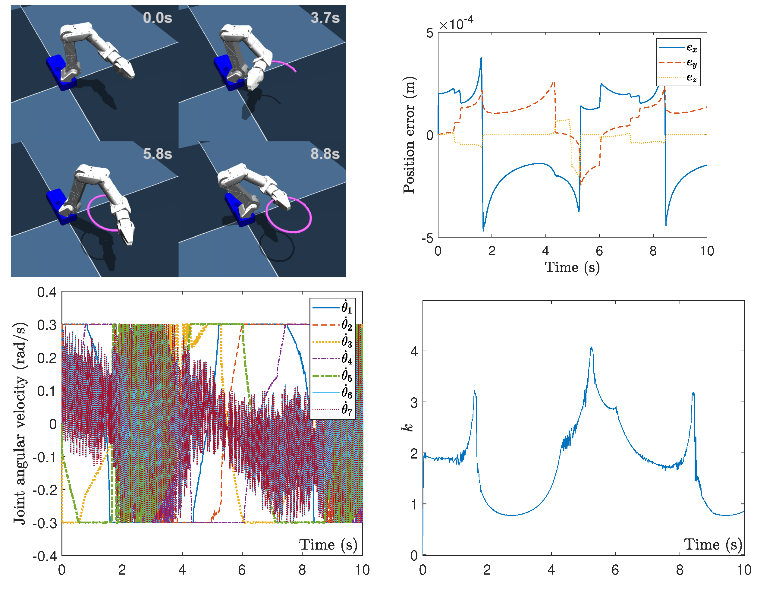
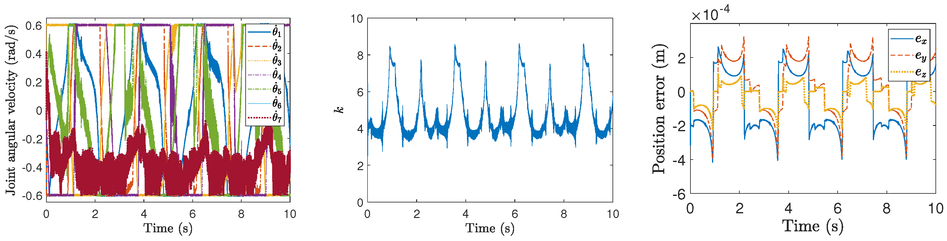
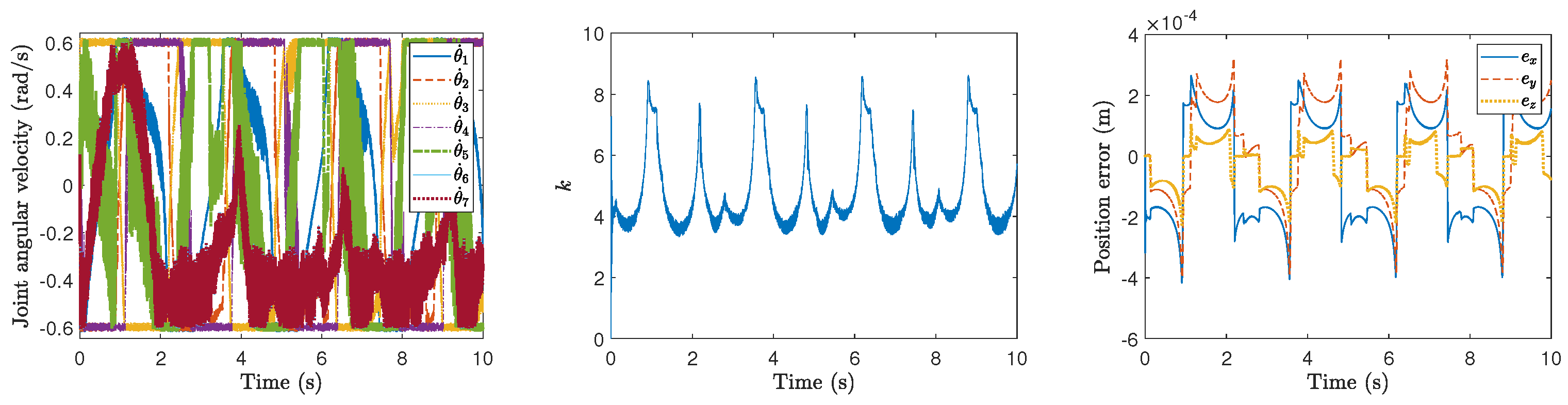
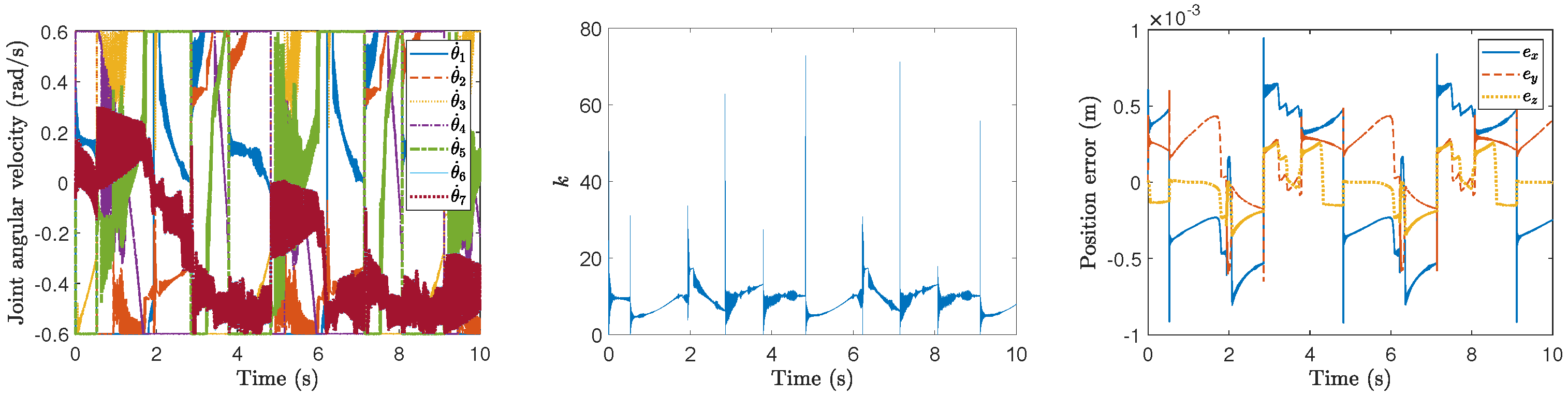
3. Simulation and Experiment Results

In this section, the proposed method is verified through simulation and experiment on a robotic manipulator, we assess and compare the effectiveness of our proposed approach with established methods/schemes and their models as well.

3.1. Simulation Verification

3.1.1. Simulation Setup

In this simulation scenario, a manipulator (called “ARM” robot) with seven degrees of freedom is used as the model for validation of the proposed method for time-optimal kinematic control against harmonic noises, and the D-H (Denavit–Hartenbeg) parameters are configured in

Table 1. Configuration of D-H table of the manipulator for simulation and experiment.

i	${\mathit{\alpha }}_{\mathit{i}-1}$ (rad)	${\mathit{a}}_{\mathit{i}-1}$ (m)	${\mathit{d}}_{\mathit{i}}$ (m)	${\mathit{\theta }}_{\mathit{i}}$ (rad)
1	0	0	0.082	${\theta }_1$
2	$\pi /2$	0.04	0	${\theta }_2$
3	0	−0.26	0	${\theta }_3+\pi /2$
4	$\pi /2$	0.0765	0.206	${\theta }_4$
5	$-\pi /2$	0	0	${\theta }_5$
6	$-\pi /2$	0	0.138	${\theta }_6$
7	$-\pi /2$	0	0	${\theta }_7$

. The task is to ensure accurate end-effector tracking of both circular and square trajectories in the workspace. In this particular context, throughout the motion planning and control phases for the manipulator, the joint velocities are consistently subject to a joint angular velocity limit of 0.3 rad/s. The maximum allocated time duration of the tracking task is set as $T_{\mathrm{task}}=12$ s. The initial joint angle ${\theta }_0$ is randomly set without exceeding its physical limit, the initial joint velocity ${\dot{\theta }}_0$ is assigned zero, and k and $\lambda$ are initialized randomly. The convergence scaling parameter is configured as $ϵ={10}^{-4}$. The disturbed harmonic noise is depicted by the following form:

$$\mathrm{Noise}=\sum _{i=1}^3{A}_i\sin (2\pi f_{i}t+{\varphi }_i)$$

with noise amplitudes being $A_1=20$, $A_2=30$ and $A_3=10$, phases being ${\varphi }_1=1.5$ Hz, ${\varphi }_2=2$ and ${\varphi }_3=5$, and frequencies being $f_1=1000$ Hz, $f_2=500$ Hz and $f_3=100$ Hz.

3.1.2. Tracking Performances

The path-tracking performance of the end-effector of the ARM manipulator by the proposed time-optimal kinematic control approach against harmonic noise is evaluated. Figure 1 and Figure 2 show comprehensive performances including path tracking accuracy and joint constraint compliance for circular and square path tracking. From the path trajectory results in Figure 1, we can observe that the manipulator by the proposed method achieves completion of the circle path tracking within 8.8 s, and the second subplot of Figure 1 shows that the tracking position error of the end-effector is within $5\times {10}^{-4}$ m. Figure 1 further illustrates the kinematic control action which is in the joint velocity level, and it can be seen that the resolved joint velocity under harmonic noises is always in the boundary $[-0.3,0.3]$ rad/s which is satisfying the joint velocity constraint from its third subplot. The time-optimal kinematic control is put to effect by dynamically maximizing the end-effector velocity through modulating the additional factor k, which is shown by the fourth subplot of Figure 1. The above results demonstrate the efficiency and accuracy of the proposed method for time-optimal kinematic control against harmonic noise in a circle path tracking task.

In addition, in Figure 2, it can be observed that the manipulator by the proposed method achieves completion of the square path tracking within 10.5 s, and the second subplot of Figure 2 indicates that the tracking position error of the end-effector is within $10\times {10}^{-4}$ m. Figure 2 also further presents the kinematic control action at the joint velocity level, and it can be seen that the resolved joint velocity under harmonic noises is always in the boundary $[-0.3,0.3]$ rad/s which is satisfying the joint velocity constraint. The time-optimal kinematic control is put to effect by dynamically maximizing the end-effector velocity through modulating the additional factor k, which is shown by the fourth subplot of Figure 2. From the results at a time instant near the end, we can observe that the variable k abruptly increases to keep the time-optimal kinematic control subject to the joint velocity constraints, as k is used as a dynamic gain switch to maximize the end-effector velocity of the manipulator. However, this process sometimes seems not smooth since no trade-off factors are involved to gently modulate the speed of the end-effector for our proposed method. These aforementioned results demonstrate the efficiency and accuracy of the proposed method for time-optimal kinematic control in square path tracking tasks. All of these path-tracking performances for two types of trajectory substantiate the effectiveness and robustness of such a time-optimal kinematic control method.

3.1.3. Comparison at Different Levels of Noises

When the harmonic noise is at different levels under different frequencies and magnitudes, we evaluate the performance of the proposed kinematic controller against the harmonic noise. In this situation, three cases are evaluated: Case (1) $A_1=20$, $A_2=30$, and $A_3=50$, and frequencies being $f_1=50$ Hz, $f_2=100$ Hz, and $f_3=200$ Hz; Case (2) $A_1=200$, $A_2=300$, and $A_3=500$, and frequencies being $f_1=1000$ Hz, $f_2=1500$ Hz, and $f_3=2000$ Hz; and Case (3) $A_1=500$, $A_2=600$, and $A_3=1000$, and frequencies being $f_1=2000$ Hz, $f_2=2500$ Hz, and $f_3=4000$ Hz. The joint velocity limits are configured as $[-0.60.6]$ rad/s, and the phases are set as ${\varphi }_1=3$, ${\varphi }_2=4$, and ${\varphi }_3=5$.

Figure 3, Figure 4, Figure 5, Figure 6, Figure 7 and Figure 8 show the motion planning and control performances of the manipulator under aforementioned harmonic noises of different levels. From these figures, we can observe that even the resolved joint velocity for kinematic control is corrupted from the harmonic noises, the position errors of the end-effector of the manipulator by the proposed time-optimal kinematic controller are within the range of ${10}^{-4}\sim {10}^{-3}$ m under these harmonic noises. Even if the magnitude and the frequency are increased to rather high values (magnitudes $\ge 500$ and frequencies $\ge 2000$ Hz), the position errors can still be small (smaller than $1\times {10}^{-3}$ m). These results validate the robustness of the proposed method for time-optimal kinematic control against harmonic noises.

It is worth mentioning here that, from Figure 6, Figure 7 and Figure 8, we can observe that, the modulating factor k often abruptly rises at some time instants during the process of time-optimal kinematic control against different levels of harmonic noises for the square path tracking. It may indicate that for such a square path tracking, the dynamic process of k is not so smoothly changing. Because k is directly used as a dynamic gain switch to maximize the end-effector velocity of the manipulator without its dynamic terms (e.g., $\dot{k}$ and/or $\ddot{k}$) together involved in the original optimization objective function, which implies that improved optimization formulation can be considered to achieve a more smooth modulation of k in the future.

Additionally, Figure 9 shows an exemplar plot of the Lagrange multipliers $\lambda$ of the proposed RNN-based approach for time-optimal kinematic control against the first level of harmonic noises for the two types of paths, and we can observe that they adaptively change over time to guarantee the time-optimal kinematic control solutions. The dynamic process of Lagrange multipliers $\lambda$ is governed by $ϵ\dot{\lambda }={\rm Y}\omega$ which is formed from the optimization paradigm for time-optimal kinematic control, and its role is not to constrain the joint velocity.

3.2. Experimental Results

3.2.1. Experiment Setup

To further verify the efficacy of the proposed method for time-optimal kinematic control against harmonic noise towards physical implementations. The time sampling rate for updating joint angles in the environment is set as 0.1 s. The maximum task time duration for the tracking task is set as $T_{\mathrm{task}}=15$ s. The initial joint angle ${\theta }_0$ is configured randomly, the initial joint velocity ${\dot{\theta }}_0$ is randomly assigned, and k and $\lambda$ are initialized randomly. The convergence scaling parameter is configured as $ϵ={10}^{-4}$. In summary, the proposed fault-tolerant method is efficient and superior for constrained time-optimal kinematic control via maximization of end-effector velocity.

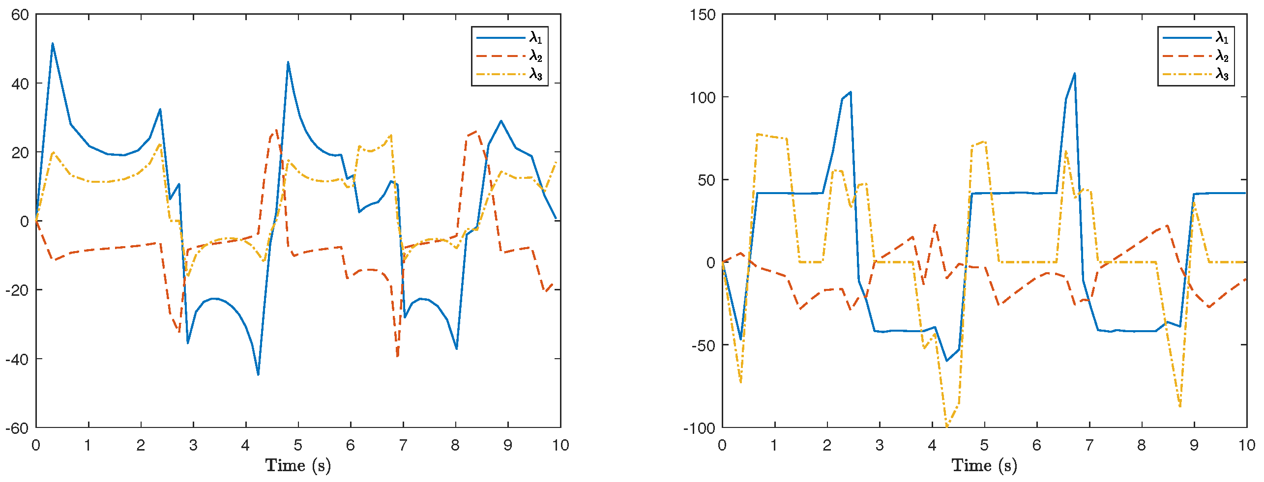
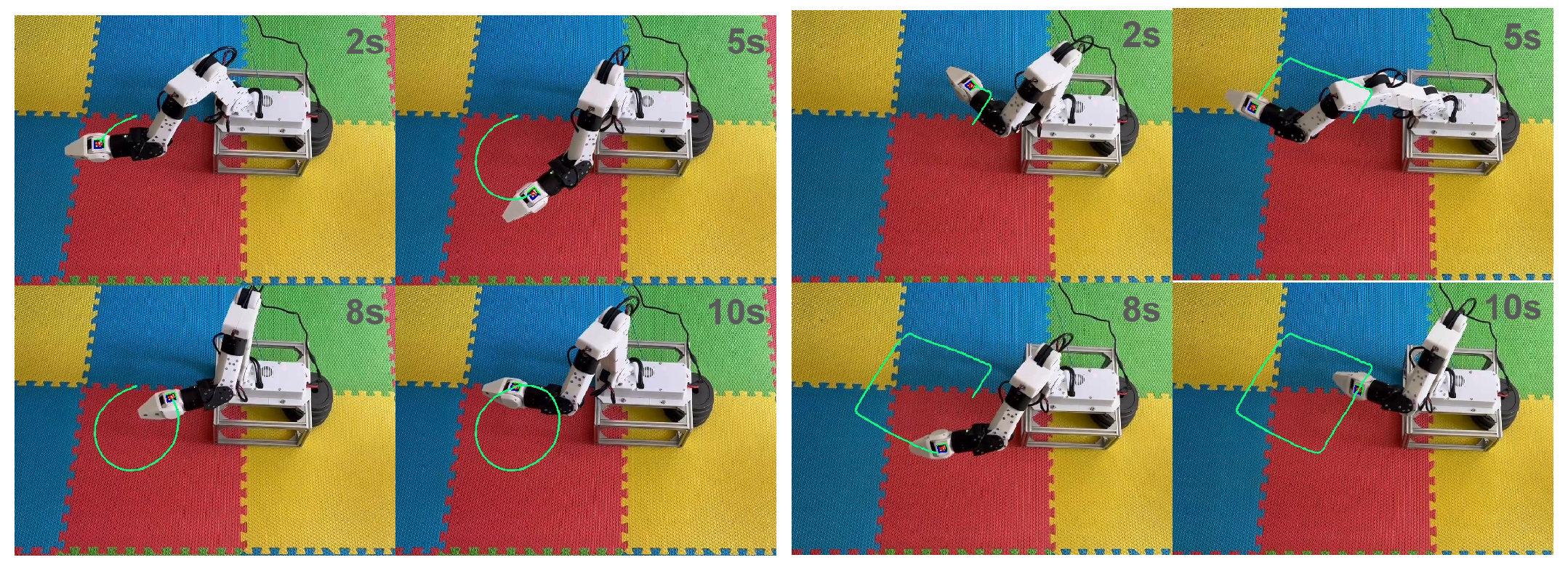
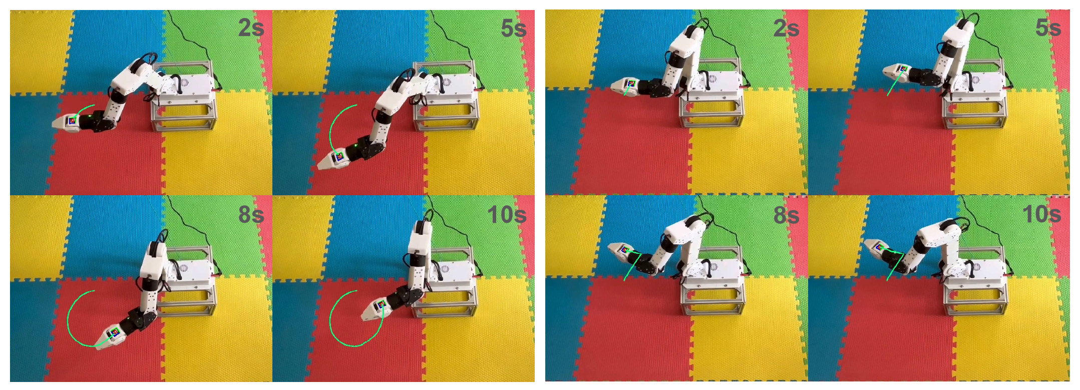
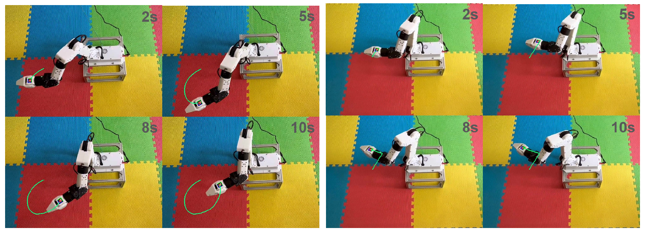
3.2.2. Tracking Performances and Comparative Study with Other Schemes

(I) Without loss of generality, the corresponding optimization problem, the constrained optimization problem for such kinematic control issue is formulated by minimizing the norm of joint velocity as follows:

$$\begin{array}{c}\hfill \begin{array}{cc}& \min {\displaystyle \frac{{\dot{\theta }}^T\dot{\theta }}{2}}\hfill \\ & \mathrm{s}.\mathrm{t}.\left\{\begin{array}{c}J\dot{\theta }-{\dot{r}}_d=0\hfill \\ \dot{\theta }\in [{\dot{\theta }}^{-},{\dot{\theta }}^{+}]\hfill \end{array}\right.\hfill \end{array}\end{array}$$

(30)

The optimization problem (30) is a convex optimization paradigm. According to the design procedures of the primal-dual neural network [23], the resultant kinematic controller based on RNN with harmonic noises can be developed as follows:

$$\left\{\begin{array}{c}\epsilon \dot{\widehat{\omega }}=-\omega +P_{\Omega }\left(J^T\lambda \right)\hfill \\ \epsilon \dot{\lambda }={\dot{r}}_d-J\omega \hfill \\ \widehat{\varphi }=-c_0ϵ-c_0{\mu }_0-ϵ\sum _{i=1}^l{\mu }_i\hfill \\ {\dot{\mu }}_0=\omega -P_{\Omega }(\omega -\chi \omega +\chi -{{\rm Y}}^T\lambda )\hfill \\ {\dot{\mu }}_i={\eta }_i+c_1(ϵ\omega +{\mu }_0)\hfill \\ {\dot{\eta }}_i=-4{\pi }^2{f}_i^2{\mu }_i\hfill \end{array}\right.$$

(31)

(II) According to [24], by incorporating a new dynamic term denoted as $\epsilon \dot{u}$, to account for joint velocity transient processes, the subsequent development of the RNN-based kinematic controller with harmonic noises is presented as follows:

$$\left\{\begin{array}{c}\epsilon \dot{\widehat{\omega }}=P_{\Omega }(J^T(r_d-r)+J^T\lambda )-\omega \hfill \\ \epsilon \dot{\lambda }={\dot{r}}_d-J{J}^T\lambda \hfill \\ \widehat{\varphi }=-c_0ϵ-c_0{\mu }_0-ϵ\sum _{i=1}^l{\mu }_i\hfill \\ {\dot{\mu }}_0=\omega -P_{\Omega }(\omega -\chi \omega +\chi -{{\rm Y}}^T\lambda )\hfill \\ {\dot{\mu }}_i={\eta }_i+c_1(ϵ\omega +{\mu }_0)\hfill \\ {\dot{\eta }}_i=-4{\pi }^2{f}_i^2{\mu }_i\hfill \end{array}\right.$$

(32)

The differences between methods (31) and (32) lie in the points as follows. Under the situation of harmonic noises, method (31) is a conventional kinematic method which tries to minimize the kinetic energy associated with joint velocity rather than handling with end-effector velocity in a workspace, and method (32) attempts to exert joint velocity compensation to enhance the kinematic control performance to get rid of noise disturbance. Both of them are utilized as comparative benchmarks to illustrate the time efficiency of the task execution for the proposed method on performing the same workspace trajectory tracking task.

Figure 10 shows the motion experimental results of our proposed method for time-optimal kinematic control of the ARM manipulator under harmonic noises. For comparison, Figure 11 and Figure 12 show the motion experimental results of other methods (31) and (32). From these results in these figures, we can observe that, under the same path tracking tasks, the proposed robust time-optimal kinematic control method is able to achieve the tracking completion within the task time 10 s. Nevertheless, the other two methods cannot guarantee path-tracking performance under the same allocated time, and their path tracking completions are getting behind with the proposed method under the same allocated task time 10 s. All of these experimental results demonstrate that our proposed method is superior to other conventional methods on such a time-optimal kinematic control issue against harmonic noises. Moreover, both the simulation and experimental results validate that, for the time-optimal kinematic control problem under harmonic noises, the proposed optimization objective function in workspace can be more efficient than those in joint space.

4. Conclusions

This paper presents a novel approach that integrates dynamic recurrent neural networks (RNNs) within a constrained optimization framework to achieve robust, time-optimal kinematic control under such noise disturbances. A comprehensive theoretical analysis establishes the convergence and optimality of the RNN-based control solver. The proposed method ensures maximum end-effector speed without violating joint velocity limits, leading to faster path tracking speed compared to conventional schemes. Simulation results and physical experiments further validate the effectiveness and superiority of the proposed approach. The proposed time-optimal kinematic control against noise disturbances can offer a robust framework with potential applications, such as enhancing the precision of robotic assembly lines by mitigating vibrational noise in high-speed pick-and-place operations, or enabling collaborative robots (cobots) to operate reliably in dynamic, noise-prone environments. Future research should focus on the following key areas to broaden the method’s impact. First, optimizing RNN’s architecture via lightweight models or hardware acceleration (e.g., FPGA/GPU integration) could reduce latency. Second, scalability studies can be extended to evaluate generalization across diverse robotic systems, such as mobile manipulators or aerial drones, by modularizing the RNN-based structure or developing adaptive parameter-tuning protocols. Third, while the current method demonstrates robustness against static harmonic noise, dynamic adaptation to varying noise spectra potentially through online learning mechanisms or adaptive noise cancellation layers remains an open question. More in-depth investigation into autonomous parameter adjustment could minimize manual tuning and expand applicability to unstructured environments, such as logistics or construction, where noise profiles evolve unpredictably (including a random type of noise). These advancements would strengthen the method’s practicality and adoption in a wider range of real-world systems.

References

1. Chen, X.; Jin, L.; Hu, B. A cerebellum-inspired control scheme for kinematic control of redundant manipulators. IEEE Trans. Ind. Electron. 2023, 71, 7539–7547. [Google Scholar] [CrossRef]
2. Zhang, Y.; Jin, L. Robot Manipulator Redundancy Resolution; John Wiley & Sons: Hoboken, NJ, USA, 2017. [Google Scholar]
3. Klein, C.A.; Huang, C.H. Review of pseudoinverse control for use with kinematically redundant manipulators. IEEE Trans. Syst. Man Cybern. 1983, SMC-13, 245–250. [Google Scholar] [CrossRef]
4. Nenchev, D.N. Redundancy resolution through local optimization: A review. J. Robot. Syst. 1989, 6, 769–798. [Google Scholar] [CrossRef]
5. Kanoun, O.; Lamiraux, F.; Wieber, P.B. Kinematic control of redundant manipulators: Generalizing the task-priority framework to inequality task. IEEE Trans. Robot. 2011, 27, 785–792. [Google Scholar] [CrossRef]
6. Liu, M.; Li, Y.; Chen, Y.; Qi, Y.; Jin, L. A distributed competitive and collaborative coordination for multirobot systems. IEEE Trans. Mob. Comput. 2024, 23, 11436–11448. [Google Scholar] [CrossRef]
7. Zhang, Y.; Ge, S.S.; Lee, T.H. A unified quadratic-programming-based dynamical system approach to joint torque optimization of physically constrained redundant manipulators. IEEE Trans. Syst. Man Cybern. Part B 2004, 34, 2126–2132. [Google Scholar] [CrossRef]
8. Xie, Z.; Jin, L.; Luo, X.; Sun, Z.; Liu, M. RNN for repetitive motion generation of redundant robot manipulators: An orthogonal projection-based scheme. IEEE Trans. Neural Netw. Learn. Syst. 2020, 33, 615–628. [Google Scholar] [CrossRef]
9. Zhang, Z.; Zhang, Y. Variable joint-velocity limits of redundant robot manipulators handled by quadratic programming. IEEE/ASME Trans. Mechatronics 2012, 18, 674–686. [Google Scholar] [CrossRef]
10. Khan, A.H.; Li, S.; Luo, X. Obstacle avoidance and tracking control of redundant robotic manipulator: An RNN-based metaheuristic approach. IEEE Trans. Ind. Inf. 2019, 16, 4670–4680. [Google Scholar] [CrossRef]
11. Jin, L.; Su, Z.; Fu, D.; Xiao, X. Coevolutionary neural solution for nonconvex optimization with noise tolerance. IEEE Trans. Neural Netw. Learn. Syst. 2023, 35, 17571–17581. [Google Scholar] [CrossRef]
12. Jin, L.; Chen, Y.; Liu, M. A noise-tolerant k-WTA model with its application on multirobot system. IEEE Trans. Ind. Inf. 2023, 20, 3574–3584. [Google Scholar] [CrossRef]
13. Li, S.; Zhou, M.; Luo, X. Modified Primal-Dual Neural Networks for Motion Control of Redundant Manipulators With Dynamic Rejection of Harmonic Noises. IEEE Trans. Neural Netw. Learn. Syst. 2018, 29, 4791–4801. [Google Scholar] [CrossRef] [PubMed]
14. Li, S.; Wang, H.; Rafique, M.U. A Novel Recurrent Neural Network for Manipulator Control With Improved Noise Tolerance. IEEE Trans. Neural Netw. Learn. Syst. 2018, 29, 1908–1918. [Google Scholar] [CrossRef]
15. Tan, N.; Yu, P.; Zhong, Z.; Ni, F. A New Noise-Tolerant Dual-Neural-Network Scheme for Robust Kinematic Control of Robotic Arms With Unknown Models. IEEE/CAA J. Autom. Sin. 2022, 9, 1778–1791. [Google Scholar] [CrossRef]
16. Zhang, Z.; Chen, S.; Deng, X.; Liang, J. A Circadian Rhythms Neural Network for Solving the Redundant Robot Manipulators Tracking Problem Perturbed by Periodic Noise. IEEE/ASME Trans. Mechatronics 2021, 26, 3232–3242. [Google Scholar] [CrossRef]
17. Li, Z.; Li, S. Time-optimal constrained kinematic control of robotic manipulators by recurrent neural network. Expert Syst. Appl. 2024, 257, 124994. [Google Scholar] [CrossRef]
18. Galicki, M. Time-optimal controls of kinematically redundant manipulators with geometric constraints. IEEE Trans. Robot. Autom. 2000, 16, 89–93. [Google Scholar] [CrossRef]
19. Reiter, A.; Müller, A.; Gattringer, H. On Higher Order Inverse Kinematics Methods in Time-Optimal Trajectory Planning for Kinematically Redundant Manipulators. IEEE Trans. Ind. Inf. 2018, 14, 1681–1690. [Google Scholar] [CrossRef]
20. Liu, G.; Li, Q.; Yang, B.; Zhang, H.; Fang, L. An Efficient Linear Programming-Based Time-Optimal Feedrate Planning Considering Kinematic and Dynamics Constraints of Robots. IEEE Robot. Autom. Lett. 2024, 9, 2742–2749. [Google Scholar] [CrossRef]
21. Yu, X.; Dong, M.; Yin, W. Time-optimal trajectory planning of manipulator with simultaneously searching the optimal path. Comput. Commun. 2022, 181, 446–453. [Google Scholar] [CrossRef]
22. He, S.; Hu, C.; Lin, S.; Zhu, Y. An Online Time-Optimal Trajectory Planning Method for Constrained Multi-Axis Trajectory With Guaranteed Feasibility. IEEE Robot. Autom. Lett. 2022, 7, 7375–7382. [Google Scholar] [CrossRef]
23. Xia, Y.S.; Feng, G.; Wang, J. A primal-dual neural network for online resolving constrained kinematic redundancy in robot motion control. IEEE Trans. Syst. Man Cybern. Part B 2005, 35, 54–64. [Google Scholar] [CrossRef] [PubMed]
24. Li, S.; Zhang, Y.; Jin, L. Kinematic control of redundant manipulators using neural networks. IEEE Trans. Neural Netw. Learn. Syst. 2016, 28, 2243–2254. [Google Scholar] [CrossRef] [PubMed]
Figure 1. Performance of the proposed method for time-optimal kinematic control against harmonic noise for the circular path.
Actuators 14 00213 g001
Figure 2. Performance of the proposed method for time-optimal kinematic control against harmonic noise for the square path.
Actuators 14 00213 g002
Figure 3. Performance of the proposed method for time-optimal kinematic control under different levels of noise for the circular path under the first level of noise.
Actuators 14 00213 g003
Figure 4. Performance of the proposed method for time-optimal kinematic control under different levels of noise for the circular path the second level of noise.
Actuators 14 00213 g004
Figure 5. Performance of the proposed method for time-optimal kinematic control under different levels of noise for the circular path under the third level of noise.
Actuators 14 00213 g005
Figure 6. Performance of the proposed method for time-optimal kinematic control under different levels of noise for the square path.
Actuators 14 00213 g006
Figure 7. Performance of the proposed method for time-optimal kinematic control under different levels of noise for the square path.
Actuators 14 00213 g007
Figure 8. Performance of the proposed method for time-optimal kinematic control under different levels of noise for the square path.
Actuators 14 00213 g008
Figure 9. Dynamic process of Lagrange multipliers λ of the RNN-based method for time-optimal kinematic control against harmonic noises for different types of noises. (Left) for the circle path tracking; (Right) for the square path tracking.
Actuators 14 00213 g009
Figure 10. Experimental performance by our proposed method for time-optimal kinematic control of ARM manipulator against harmonic noises. The circle and square path tracking tasks are accomplished in the task time 10 s.
Actuators 14 00213 g010
Figure 11. Experimental performance by method (31) for time-optimal kinematic control of ARM manipulator against harmonic noises. The circle and square path tracking tasks cannot be finished within task time 10 s.
Actuators 14 00213 g011
Figure 12. Experimental performance by method (32) for time-optimal kinematic control of ARM manipulator against harmonic noises. The circle and square path tracking tasks cannot be finished within task time 10 s.
Actuators 14 00213 g012