Connected and Automated Vehicle Trajectory Control in Stochastic Heterogeneous Traffic Flow with Human-Driven Vehicles Under Communication Delay and Disturbances

Abstract

In this paper, we study the stability of the stochastically heterogeneous traffic flow involving connected and automated vehicles (CAVs) and human-driven vehicles (HDVs). Taking the stochasticity of vehicle arrivals and behaviors into account, a general robust $H_{\infty }$ platoon controller is proposed to address the communication delay and unexpected disturbances such as prediction or perception errors on HDV motions. To simplify the problem complexity from a stochastically heterogeneous traffic flow to multiple long vehicle control problems, three types of sub-platoons are identified according to the CAV arrivals, and each sub-platoon can be treated as a long vehicle. The car-following behaviors of HDVs and CAVs are simulated using the optimal velocity model (OVM) and the cooperative adaptive cruise control (CACC) system, respectively. Later, the robust $H_{\infty }$ platoon controller is designed for a pair of a CAV long vehicle and an HDV long vehicle. The time-lagged system and the closed-loop system are formulated and the $H_{\infty }$ state feedback controller is designed. The robust stability and string stability of the heterogeneous platoon system are analyzed using the $H_{\infty }$ norm of the closed-loop transfer function and the time-lagged bounded real lemma, respectively. Simulation experiments are conducted considering various settings of platoon sizes, communication delays, disturbances, and CAV penetration rates. The results show that the proposed $H_{\infty }$ controller is robust and effective in stabilizing disturbances in the stochastically heterogeneous traffic flow and is scalable to arbitrary sub-platoons in various CAV penetration rates in the heterogeneous traffic flow of road vehicles. The advantages of the proposed method in stabilizing heterogeneous traffic flow are verified in comparison with a typical car-following model and the linear quadratic regulator.

1. Introduction

Enabled by vehicle-to-vehicle (V2V) communication, connected and automated vehicles (CAVs) can be regulated in platoons for a common goal of improving traffic efficiency for less travel delay and energy consumption, such as the cooperative adaptive cruise control (CACC) system. However, the external disturbances on vehicle dynamics and communication delay degrade the performance of the CAV platoons [1].

Various control approaches are employed to counteract the uncertainties caused by external disturbances and communication delays in the homogeneous and heterogeneous traffic flows, such as the optimal control approaches and the robust control approaches. The optimal control approaches, which apply a fixed control law in an open loop, can address communication delays and stabilize the heterogeneous traffic flow to verify traffic stability [2] or to minimize velocity disturbances in the human-dominated traffic flow [3]. Nevertheless, these optimal control methods often neglect system uncertainty and dynamic changes.

To address these limitations, various robust control methods have been developed to improve performance under uncertainties and dynamic disturbances, such as robust model predictive control (MPC), car-following strategies, cooperative or adaptive control, and $H_{\infty }$ control. In the field of robust MPC, the tube-based robust MPC approaches have been proposed by Feng et al. [4] and Yin et al. [5] to manage prediction uncertainties and stabilize homogeneous platoons. Zhou et al. [6] further designed a robust min-max MPC with disturbance feedback to mitigate external disturbances for a homogeneous platoon. The robust car-following control strategies have been developed by Zhou et al. [7] and Li et al. [8] to improve the CAV stability and platoon performance under uncertainties and delays. Multiple cooperative and adaptive control methods have been proposed to enhance homogeneous platoon performance and stability considering delays and disturbances. For instance, Wang et al. [9,10] have formulated the robust cooperative control strategies as a min-max problem to address sensor or control errors despite uncertain vehicle dynamics. Zhao et al. [11] have proposed a robust safety-critical traffic control method that prioritizes safety over stability, and Sun et al. [12] have developed an artificial bee colony algorithm within an adaptive robust control framework, both used to counteract external disturbances. While these methods above significantly enhance the stability and performance of CAV platoon control systems in homogeneous traffic flows, not all approaches take traffic flow heterogeneity into account when addressing platoon stability.

To take the uncertain human-driven vehicle (HDV) motions into account, Swaroop et al. [13] have widely studied the robust $H_{\infty }$ control approaches for string stability in heterogeneous traffic flows. The decoupled robust $H_{\infty }$ control method for the heterogeneous platoon with uncertain disturbances has been proposed by Li et al. [14] to ensure string stability. Monteil et al. [15] have designed the $H_{\infty }$ control strategy with linear matrix inequality constraints to diminish disturbances resulting from HDVs by maximizing the string stability of the heterogeneous traffic flow. The $H_{\infty }$ dynamic output feedback controllers have been designed by Wang et al. [16] and Mousavi et al. [17] to address the controllability and stabilizability of a heterogeneous traffic system with HDV disturbances. Zhou et al. [18] and Wang et al. [19] have both proposed the robust control approaches for string stability considering HDV disturbances, which treats the $H_{\infty }$ norm of the heterogeneous platoons as the control objective. Orki et al. [20] have designed the $H_{\infty }$ controller to handle the challenges caused by disturbed HDVs in heterogeneous traffic flows. Although the $H_{\infty }$ control methods above demonstrate the stability of the heterogeneous traffic flow considering the external disturbances of HDV dynamics, they exclude the stochasticity in the vehicle sequence and communication delays.

To compensate for communication delays in the based $H_{\infty }$ control approach, Hajdu et al. [21] have developed the $H_{\infty }$ control framework for string stability to counteract external disturbances considering the communication latency. Later, Halder et al. [22,23] designed the $H_{\infty }$ state feedback controllers for a platoon system to mitigate the effects of external disturbances and communication delays using the undirected topology and the linear matrix inequalities. Liu et al. [24] have proposed the novel $H_{\infty }$ pinning approach for a multi-delay complex network with external disturbances. The robust $H_{\infty }$ control scheme has been proposed by Gong et al. [25] to stabilize heterogeneous traffic systems against disturbances and communication delays considering different car-following modes. Elahi et al. [26] have proposed the fixed-time $H_{\infty }$ consensus control protocol for heterogeneous platoons to mitigate the adverse effects of disturbances and multiple transmission delays. However, these studies neglect the influence of stochastic vehicle sequences, which may challenge the generality and scalability of the proposed $H_{\infty }$ approaches in the stochastically real traffic flow.

From the discussion above, it can be concluded that current research on platoon control in the heterogeneous traffic flow rarely incorporates communication delays and the stochasticity of vehicle arrivals (i.e., vehicle sequence in the platoon) simultaneously. To this end, this paper designs a robust $H_{\infty }$ controller for the stochastically heterogeneous traffic flow considering communication delay and external disturbances such as prediction errors of HDV motions. To reduce the complexity of the control problem, the stochastically heterogeneous traffic flow is divided into multiple sub-platoons based on the CAV sequence. Each sub-platoon can be treated as a long vehicle by assuming homogeneity within the sub-platoon. This approach reduces the propagation of disturbances within the platoon, thereby decreasing the sensitivity of the overall system to external disturbances and facilitating the analysis of the string stability of the platoon system. The optimal velocity model (OVM) and the CACC system are applied in the robust $H_{\infty }$ controller design to describe the car-following behaviors of HDVs and CAVs, respectively. The prediction errors and unexpected motions of HDVs are treated as external disturbances affecting deviations in HDV accelerations. The $H_{\infty }$ norm is applied to design the state feedback controller, followed by analyzing the robust and string stability of the robust platoon controller. The controller performance is verified by simulation of eleven experiments, considering various platoon sizes, communication delays, prediction errors of HDV motions, and CAV penetration rates in the heterogeneous traffic flows. The results show that the $H_{\infty }$ controller can effectively reduce traffic oscillations in the heterogeneous traffic flow and adapt to different penetration rates of CAVs in various settings of platoon sizes, communication delays, and external disturbances. The comparative results verify the robustness and effectiveness of the proposed controller compared with the Intelligent Driver Model (IDM) and Linear Quadratic Regulator (LQR) controller. Finally, the differences in behaviors between CAVs and HDVs are summarized based on the simulation results.

The rest of this paper is organized as follows. Section 2 describes the control problem and defines the mathematical notations. Section 3 presents the vehicle dynamics models for individual HDVs and individual CAVs and then designs the $H_{\infty }$ controller for a pair of long vehicles (i.e., an HDV sub-platoon and a CAV sub-platoon) in the heterogeneous traffic flow with communication delays and disturbances. Section 4 analyzes the robust stability and the string stability of a pair of long vehicles in the heterogeneous traffic flow. Section 5 proposes the solution approach to the robust $H_{\infty }$ controller for the heterogeneous platoon considering communication delay and disturbances. Section 6 conducts experimental simulation and analyzes the simulation results. Finally, we conclude this paper and discuss the future work in Section 7.

2. Problem Description

This paper studies the CAVs and HDVs in a heterogeneous traffic flow within the communication range, namely the overall heterogeneous platoon. All vehicles travel on the road without a centralized external traffic control, and the stochastic vehicle sequence in the overall platoon is known. The heterogeneous platoon system is assumed to be equipped with basic on-board sensors and V2V communication capabilities for information exchange. HDVs can connect with CAVs via V2V communication. However, the desired acceleration is not immediately realized due to communication delays in the transfer of information between vehicles. Deviations and prediction errors in HDV motions (such as accelerations) are treated as external disturbances. To simplify the control problem and minimize disturbance propagation within the platoon, the overall heterogeneous platoon is segmented into multiple sub-platoons and each sub-platoon can be treated as a long vehicle, assuming the homogeneity of member vehicles in the sub-platoon, as discussed below.

The platoon and sub-platoon identification is demonstrated in Figure 1. Here, i and k denote the indexes of the individual vehicle and the long vehicle (i.e., sub-platoon), respectively. $I_k$ is the vehicle set of a long vehicle. In Figure 1, the individual vehicles and the long vehicles are represented as solid and dashed rectangles, respectively. In the overall heterogeneous platoon, CAVs and HDVs constitute a heterogeneous traffic flow with a stochastic quantity and sequence of CAVs and HDVs. The sub-platoon is defined by consecutively homogeneous vehicles. With the assumption of leading CAV sub-platoon $I_1$, each following CAV sub-platoon $I_k$ is assigned an odd-numbered index $k=2\rho +1$ given a positive integer $\rho$. Each following HDV sub-platoon is indexed by an even-number $I_{2\rho }$. For simplicity, it is assumed that the leading CAV sub-platoon $I_1$ travels at a constant desired velocity ${\mathbf{v}}^{*}$, and other CAV sub-platoons follow a designed control method to reach the target acceleration.

Each sub-platoon $I_k$ can be treated as a long vehicle due to its vehicle homogeneity. Therefore, the entire heterogeneous platoon can be simplified by segmenting into the leading CAV long vehicle $I_1$, the following HDV long vehicles $I_{2\rho }$, and the following CAV long vehicles $I_{2\rho +1}$. Each controlled CAV long vehicle adjusts its acceleration based on the input from the following HDV long vehicle to stabilize the subsequent vehicles. Let $\rho$ ($\in {\mathbb{Z}}^{+}$) denote the index of each pair of long vehicles, which includes a following HDV long vehicle $I_{2\rho }$ and a following CAV long vehicle $I_{2\rho +1}$. As depicted in Figure 1, the overall heterogeneous platoon can be described by a leading CAV long vehicle followed by multiple pairs of long vehicles, with each pair comprising a following HDV long vehicle $I_{2\rho }$ and a following CAV long vehicle $I_{2\rho +1}$. The $H_{\infty }$ control design for a pair of long vehicles can be applied to all pairs in the platoon.

In this paper, the normal and bold notations are applied to represent variables and vectors for individual vehicles (v, x, u, w, y and z) and long vehicles ($\mathbf{v}$, $\mathbf{x}$, $\mathbf{u}$, $\mathbf{w}$, $\mathbf{y}$, and $\mathbf{z}$), respectively. $\mathbb{I}$ is the unit matrix with the appropriate dimensions, and $\mathrm{diag}\{\dots \}$ denotes the diagonal matrix. For the time-varying vector $\varphi \left(t\right)\in {\mathbb{R}}^n$, ${\parallel \varphi \left(t\right)\parallel }_2$ denotes its ${\mathcal{L}}_2$-norm given by ${\parallel \varphi \left(t\right)\parallel }_2={\left({\int }_0^{+\infty }{\varphi }^{\mathrm{T}}\left(t\right)\varphi \left(t\right)\mathrm{d}t\right)}^{1/2}$, and ${\mathcal{L}}_2$$[0,+\infty )$ is the space of the square-integrable vector functions $\varphi \left(t\right)$. ${\parallel \varphi \left(t\right)\parallel }_{\infty }=\underset{t}{sup}\parallel \varphi \left(t\right)\parallel$ denotes its $H_{\infty }$ norm. The symbol ∗ in a matrix denotes the symmetric structure and transpose term of the matrix, e.g., $\left[\begin{array}{cc}A& B\\ & C\end{array}\right]=\left[\begin{array}{cc}A& B\\ B^{\mathrm{T}}& C\end{array}\right].$

3. Heterogeneous Traffic Flow Control

In this section, the vehicle dynamics models for HDVs and CAVs in the sub-platoon are presented in Section 3.1 and Section 3.2, respectively. In Section 3.3, the robust control design for a pair of long vehicles in the heterogeneous traffic flow with communication delays and disturbances is proposed.

3.1. HDV Modeling

The position and velocity of the i-th HDV are denoted as $p_i\left(t\right)$ and $v_i\left(t\right)$. The distance between vehicle i and $i-1$ ($i>1$) is denoted by $z_i\left(t\right)=p_{i-1}\left(t\right)-p_i\left(t\right)$ with t representing time. The dynamic equations for the HDVs are expressed as follows:

$${\dot{z}}_i\left(t\right)=v_{i-1}\left(t\right)-v_i\left(t\right),$$

(1)

$${\dot{v}}_i\left(t\right)=F_i(v_i\left(t\right),z_i\left(t\right),{\dot{z}}_i\left(t\right)),i\in I_k,k=2\rho ,\rho \in {\mathbb{Z}}^{+}.$$

(2)

The increase in model parameters will add difficulty and degrade the accuracy of parameter estimation [17]. Therefore, the nonlinear function $F_i(·)$ of the OVM is selected to model HDV behaviors in the sub-platoon ($i\in I_{2\rho }$) owing to the simplicity of the OVM [27]:

$$F_i\left(v_i\left(t\right),z_i\left(t\right),{\dot{z}}_i\left(t\right)\right)=\alpha \left[V\left(z_i\left(t\right)\right)-v_i\left(t\right)\right]+\beta {\dot{z}}_i\left(t\right),$$

(3)

where $\alpha$ and $\beta$ are the degrees of the vehicle response to velocity differences. $V\left(z_i\left(t\right)\right)$ is the desired velocity. The equilibrium point $(z^{*},v^{*})$ of the dynamics is reached if the vehicle keeps the equilibrium velocity $v^{*}$ and the equilibrium spacing $z^{*}$, defined by Equation (2) as $F(v^{*},z^{*},0)=0$. The control states are the deviation from the equilibrium spacing ${\overline{z}}_i\left(t\right)$ and the deviation from the equilibrium velocity ${\overline{v}}_i\left(t\right)$. The mentioned control states are given with the following equations:

$$x_i\left(t\right)=\left[\begin{array}{c}{\overline{z}}_i\left(t\right)\\ {\overline{v}}_i\left(t\right)\end{array}\right],$$

(4)

$${\overline{z}}_i\left(t\right)=z_i\left(t\right)-z^{*}\left(t\right),$$

(5)

$${\overline{v}}_i\left(t\right)=v_i\left(t\right)-v^{*}\left(t\right).$$

(6)

To facilitate smooth traffic flow, the desired velocity $V\left(z_i\left(t\right)\right)$ is represented as a continuous piecewise function; see below.

$$\begin{array}{c}\hfill V\left(z_i\left(t\right)\right)=\left\{\begin{array}{cc}0,& z_i\left(t\right)\le z_{\min }\\ f_v\left(z_i\left(t\right)\right),& z_{\min }\le z_i\left(t\right)\le z_{\max }\\ v_{max},& z_i\left(t\right)\ge z_{\max }\end{array}\right.,\end{array}$$

(7)

where the desired velocity $V\left(z_i\left(t\right)\right)$ is set to zero at the minimum spacing $z_{min}$ and attains a maximum value $v_{max}$ at the maximum spacing $z_{max}$. The monotonically increasing function $f_v\left(z_i\left(t\right)\right)$ determines the desired velocity for spacing values $z_i\left(t\right)$ that fall between $z_{min}$ and $z_{max}$. A common choice of $f_v\left(z_i\left(t\right)\right)$, which is selected in this paper, is expressed as:

$$\begin{array}{c}\hfill f_v\left(z_i\left(t\right)\right)={\displaystyle \frac{v_{max}}{2}}\left(1-cos\left(\pi {\displaystyle \frac{z_i\left(t\right)-z_{min}}{z_{max}-z_{min}}}\right)\right).\end{array}$$

(8)

For the nonlinear function of the general OVM model given by Equation (3), the following equilibrium point $(z^{*},v^{*})$ can be determined by satisfying the condition $F(v^{*},z^{*},0)=0$.

$$\begin{array}{c}\hfill v^{*}=V\left(z^{*}\right).\end{array}$$

(9)

Linearizing Equation (1) around the equilibrium point gives

$${\dot{\overline{z}}}_i\left(t\right)={\overline{v}}_{i-1}\left(t\right)-{\overline{v}}_i\left(t\right).$$

(10)

Linearizing Equation (3) and applying the Taylor series expansion, we have

$$a_i\left(t\right)={\dot{\overline{v}}}_i\left(t\right)=-\left({\eta }_1+{\eta }_3\right){\overline{v}}_i\left(t\right)+{\eta }_2{\overline{z}}_i\left(t\right)+{\eta }_3{\overline{v}}_{i-1}\left(t\right),$$

(11)

where

$${\eta }_1=-{\displaystyle \frac{\partial F_i}{\partial v_i}},{\eta }_2={\displaystyle \frac{\partial F_i}{\partial z_i}},{\eta }_3={\displaystyle \frac{\partial F_i}{\partial {\dot{z}}_i}},$$

(12)

and ${\eta }_1$, ${\eta }_2$, and ${\eta }_3$ are weights on the deviation from the equilibrium velocity, the deviation from the equilibrium spacing, and the velocity difference of the HDVs, respectively. These weights can be obtained by applying a first-order Taylor expansion at the equilibrium point $(z^{*},v^{*})$ by Equation (3). Substituting the weights into Equation (9), we have

$${\eta }_1=\alpha ,{\eta }_2=\alpha \dot{V}\left(z^{*}\right),{\eta }_3=\beta ,$$

(13)

where $\dot{V}\left(z^{*}\right)$ represents the derivative of $V\left(z_i\left(t\right)\right)$ for $z_i\left(t\right)$ evaluated at the equilibrium spacing $z^{*}$.

3.2. CAV Modeling

It is assumed that the leading CAV sub-platoon $I_1$ travels at a specific desired velocity $v^{*}$. For the other following CAV sub-platoons ($i\in I_{2\rho +1}$), the car-following behaviors of CAVs in the sub-platoon are modeled using the CACC model [28], as given with the following equations:

$${\overline{z}}_i\left(t\right)=z_i\left(t\right)-z^{*}\left(t\right)=z_i\left(t\right)-T_{\mathrm{c}}{v}_i\left(t\right),$$

(14)

$$v_i(t+1)=v_i\left(t\right)+k_{\mathrm{p}}{\overline{z}}_i(t+1)+k_{\mathrm{v}}{\dot{\overline{z}}}_i(t+1),i\in I_k,k=2\rho +1,\rho \in {\mathbb{Z}}^{+},$$

(15)

where ${\overline{z}}_i\left(t\right)$ represents the deviation from the equilibrium spacing. $z^{*}\left(t\right)$ is the equilibrium spacing. $T_{\mathrm{c}}$ is the safe time headway, typically 2 s. $k_{\mathrm{p}}$ and $k_{\mathrm{v}}$ represent the regulation coefficients for the position difference and velocity difference of the CAV, which are usually taken as 0.23 and 0.07, respectively. $k_{\mathrm{p}}$ and $k_{\mathrm{v}}$ are integrated into the control parameters to regulate the velocity and acceleration of the CAV through the designed robust $H_{\infty }$ controller.

Equation (16) is obtained by taking the derivative of Equation (14). Substituting Equation (16) into Equation (15), we have Equation (17) as follows:

$$\begin{array}{c}\hfill {\dot{\overline{z}}}_i\left(t\right)=v_{i-1}\left(t\right)-v_i\left(t\right)-T_{\mathrm{c}}{a}_i\left(t\right),\end{array}$$

(16)

$$\begin{array}{c}\hfill v_i\left(t\right)-v_i\left(t-1\right)+k_v{T}_{\mathrm{c}}{a}_i\left(t\right)=k_p{\overline{z}}_i\left(t\right)+k_v\Delta v_i\left(t\right),\end{array}$$

(17)

where $\Delta v_i\left(t\right)$ ($i>1$) denotes the difference in velocity between ($i-1$)-th vehicle and i-th vehicle. Based on the simplification of Equation (17), the CAV acceleration can be calculated as Equation (18).

$$a_i\left(t\right)={\displaystyle \frac{k_p{\overline{z}}_i\left(t\right)+k_v\Delta v_i\left(t\right)}{\Delta t+k_v{T}_{\mathrm{c}}}},$$

(18)

where $\Delta t$ denotes the time interval. To facilitate linearization, Equation (14) is substituted into Equation (18), and we then obtain Equation (19); see below.

$$\begin{array}{c}\hfill a_i\left(t\right)=-{\displaystyle \frac{k_{\mathrm{p}}{T}_{\mathrm{c}}}{\Delta t+k_{\mathrm{v}}{T}_{\mathrm{c}}}}{v}_i\left(t\right)+{\displaystyle \frac{k_{\mathrm{p}}}{\Delta t+k_{\mathrm{v}}{T}_{\mathrm{c}}}}{z}_i\left(t\right)+{\displaystyle \frac{k_{\mathrm{v}}}{\Delta t+k_{\mathrm{v}}{T}_{\mathrm{c}}}}{\dot{z}}_i\left(t\right).\end{array}$$

(19)

By linearizing Equation (19) using a first-order Taylor expansion at the equilibrium point $(z^{*},v^{*})$, we can obtain a linearized CAV acceleration model which contains the deviation from the equilibrium spacing ${\overline{z}}_i\left(t\right)$ and the deviation from the equilibrium velocity ${\overline{v}}_i\left(t\right)$, as follows:

$$a_i\left(t\right)=-({\delta }_1+{\delta }_3){\overline{v}}_i\left(t\right)+{\delta }_2{\overline{z}}_i\left(t\right)+{\delta }_3{\overline{v}}_{i-1}\left(t\right),$$

(20)

and the ${\delta }_i$ weights are obtained with:

$${\delta }_1={\displaystyle \frac{k_{\mathrm{p}}{T}_{\mathrm{c}}+T_{\mathrm{c}}-k_{\mathrm{v}}{T_{\mathrm{c}}}^2}{\Delta t+k_{\mathrm{v}}{T}_{\mathrm{c}}}},{\delta }_2={\displaystyle \frac{k_{\mathrm{p}}}{\Delta t+k_{\mathrm{v}}{T}_{\mathrm{c}}}},{\delta }_3={\displaystyle \frac{k_{\mathrm{v}}}{\Delta t+k_{\mathrm{v}}{T}_{\mathrm{c}}}}.$$

(21)

Here, ${\delta }_1$, ${\delta }_2$, and ${\delta }_3$ are weights on the deviation from the equilibrium velocity, the deviation from the equilibrium spacing, and the velocity difference of the CAVs, respectively.

3.3. $H_{\infty }$ Control Design of the Long Vehicles

The control systems for the HDV sub-platoon and the CAV sub-platoon are formulated in Equations (11) and (20), either of which can be regarded as a long vehicle by neglecting the differences of the member vehicles in the sub-platoon. In this section, the variables for the long vehicle control system are represented in bold to differentiate from the individual vehicle control systems in Section 3.1 and Section 3.2. As shown in Figure 1, the overall heterogeneous platoon can be regarded as a leading CAV long vehicle followed by multiple long vehicle pairs, and each pair consists of a following HDV long vehicle and a following CAV long vehicle. Hereinafter, a pair of long vehicles including the following HDV long vehicle $I_{2\rho }$ and the following CAV long vehicle $I_{2\rho +1}$ are exemplified in the $H_{\infty }$ control design. The same control design can also be applied to the other pairs of long vehicles.

The state vector for the long vehicle $I_k$ is defined as ${\mathbf{x}}_k\left(t\right)={[{\overline{\mathbf{z}}}_k\left(t\right),{\overline{\mathbf{v}}}_k\left(t\right)]}^{\mathrm{T}}$ ($k\in {\mathbb{Z}}^{+}$). The leading CAV long vehicle $I_1$ is assumed to travel at the desired velocity ${\mathbf{v}}^{*}$. The state vector for the following HDV long vehicle $I_{2\rho }$ and the following CAV long vehicle $I_{2\rho +1}$ is $\mathbf{x}\left(t\right)={[{\mathbf{x}}_{2\rho }^{\mathrm{T}}\left(t\right),{\mathbf{x}}_{2\rho +1}^{\mathrm{T}}\left(t\right)]}^{\mathrm{T}}$. The control input $\mathbf{u}\left(t\right)$ of the following CAV long vehicle $I_{2\rho +1}$ is the desired acceleration ${\mathbf{a}}_{2\rho +1}\left(t\right)$. The variation in accelerations of the preceding HDV long vehicle is treated as the disturbance $\mathbf{w}\left(t\right)$. The communication delay among long vehicles is incorporated in the dynamics model as follows:

$${\mathbf{a}}_{2\rho }\left(t\right)=-({\eta }_1+{\eta }_3){\overline{\mathbf{v}}}_{2\rho }(t-\tau )+{\eta }_2{\overline{\mathbf{z}}}_{2\rho }(t-\tau )+{\eta }_3{\overline{\mathbf{v}}}_{2\rho -1}(t-\tau ),$$

(22)

$$\mathbf{u}\left(t\right)=-({\delta }_1+{\delta }_3){\overline{\mathbf{v}}}_{2\rho +1}(t-\tau )+{\delta }_2{\overline{\mathbf{z}}}_{2\rho +1}(t-\tau )+{\delta }_3{\overline{\mathbf{v}}}_{2\rho }(t-\tau ),$$

(23)

where $\tau$ ($0\le \tau \le \overline{\tau }$) is the communication delay among long vehicles $I_k$. $\overline{\tau }$ is the maximum communication delay. The state vector set of the following HDV long vehicle $I_{2\rho }$ and the following CAV long vehicle $I_{2\rho +1}$ with communication delay is defined as:

$$\mathbf{x}(t-\tau )=\left[\begin{array}{c}{\mathbf{x}}_{2\rho }^{\mathrm{T}}(t-\tau )\\ {\mathbf{x}}_{2\rho +1}^{\mathrm{T}}(t-\tau )\end{array}\right].$$

(24)

Therefore, the control system for a pair of long vehicles in the heterogeneous traffic flow with communication delays and disturbances can be described using the following time-lagged system.

$$\left\{\begin{array}{c}\dot{\mathbf{x}}\left(t\right)=A\mathbf{x}\left(t\right)+A_{\tau }\mathbf{x}\left(t-\tau \right)+B\mathbf{u}\left(t\right)+B_{\mathrm{w}}\mathbf{w}\left(t\right),\hfill \\ \mathbf{z}\left(t\right)=C_{\mathrm{z}}\mathbf{x}\left(t\right)+D_{\mathrm{z}}\mathbf{u}\left(t\right),\hfill \\ \mathbf{y}\left(t\right)=C\mathbf{x}\left(t\right),\hfill \end{array}\right.$$

(25)

where

$$\begin{array}{cc}\hfill A& =\left[\begin{array}{cccc}0& -1& 0& 0\\ 0& 0& 0& 0\\ 0& 1& 0& -1\\ 0& 0& 0& 0\end{array}\right],A_{\tau }=\left[\begin{array}{cccc}0& 0& 0& 0\\ {\eta }_2& -{\eta }_1-{\eta }_3& 0& 0\\ 0& 0& 0& 0\\ 0& 0& 0& 0\end{array}\right],\hfill \\ \hfill B& =\left[\begin{array}{c}0\\ 0\\ -T_{\mathrm{c}}\\ 1\end{array}\right],B_{\mathrm{w}}=\left[\begin{array}{c}0\\ 1\\ 0\\ 0\end{array}\right],C=\left[\begin{array}{cccc}1& 0& 0& 0\\ 0& 1& 0& 0\\ 0& 0& 1& 0\\ 0& 0& 0& 1\end{array}\right].\hfill \end{array}$$

(26)

Since the full state of the system is observable, the $\mathbf{x}\left(t\right)$ can be obtained by numerical computation. The parameters ${\mu }_{\mathrm{z}}$, ${\mu }_{\mathrm{v}}$, and ${\mu }_{\mathrm{u}}$ denote the weights associated with the spacing difference, the velocity difference, and the control inputs, respectively. The tuned output of the system can be expressed as:

$$\mathbf{z}\left(t\right)={\mu }_{\mathrm{z}}{\overline{\mathbf{z}}}_{2\rho }\left(t\right)+{\mu }_{\mathrm{v}}{\overline{\mathbf{v}}}_{2\rho }\left(t\right)+{\mu }_{\mathrm{z}}{\overline{\mathbf{z}}}_{2\rho +1}\left(t\right)+{\mu }_{\mathrm{v}}{\overline{\mathbf{v}}}_{2\rho +1}\left(t\right)+{\mu }_{\mathrm{u}}\mathbf{u}\left(t\right).$$

(27)

Therefore, we can obtain $C_{\mathrm{z}}=\left[{\mu }_{\mathrm{z}},{\mu }_{\mathrm{v}},{\mu }_{\mathrm{z}},{\mu }_{\mathrm{v}}\right]$ and $D_{\mathrm{z}}={\mu }_{\mathrm{u}}$. The time-lagged system Equation (25) aims to find a state output-feedback controller $\mathbf{u}\left(t\right)=K\mathbf{y}(t-\tau )$ that enables the system (25) to minimize the effect of the disturbance $\mathbf{w}\left(t\right)$ on the tuned output $\mathbf{z}\left(t\right)$. The controller $\mathbf{u}\left(t\right)$ is expressed as follows:

$$\mathbf{u}\left(t\right)=K\mathbf{y}\left(t-\tau \right)=KC\mathbf{x}\left(t-\tau \right),$$

(28)

with gain $K\in {\mathbb{R}}^{1\times n}$. Substituting Equation (28) with Equation (25), the closed-loop system of the heterogeneous platoon is obtained as follows:

$$\left\{\begin{array}{c}\dot{\mathbf{x}}\left(t\right)=A\mathbf{x}\left(t\right)+\widehat{B}\mathbf{x}\left(t-\tau \right)+B_{\mathrm{w}}\mathbf{w}\left(t\right),\hfill \\ \mathbf{z}\left(t\right)=C_{\mathrm{z}}\mathbf{x}\left(t\right)+\widehat{D}\mathbf{x}\left(t-\tau \right),\hfill \end{array}\right.$$

(29)

where $\widehat{B}=A_{\tau }+BKC$ and $\widehat{D}=D_{\mathrm{z}}KC$. Two lemmas are introduced for the stability analysis in Section 4.

Lemma 1

([29]). (Schur complement) For a given symmetric matrix $S^{\mathrm{T}}=\left[\begin{array}{cc}{S}_{11}& S_{12}\\ & S_{22}\end{array}\right]$ where $S_{11}\in {\mathbb{R}}^{n\times n}$, the following conditions are equivalent: (1) $S<0$; (2) $S_{11}<0$ and $S_{22}-S_{12}^{\mathrm{T}}{S}_{11}^{-1}{S}_{12}<0$; (3) $S_{22}>0$ and $S_{11}+S_{12}{S}_{22}^{-1}{S}_{21}<0$.

Lemma 2

([30]). For given matrices $Q=Q^{\mathrm{T}}$, H, and E with appropriate dimensions, the matrix inequality $Q+HF\left(t\right)E+E^{\mathrm{T}}{F}^{\mathrm{T}}\left(t\right)H^{\mathrm{T}}<0$ holds for all $F\left(t\right)$ satisfying $F^{\mathrm{T}}\left(t\right)F\left(t\right)\le \mathbb{I}$ if and only if there exists $\epsilon >0$ such that $Q+{\epsilon }^{-1}H{H}^{\mathrm{T}}+\epsilon E^{\mathrm{T}}E<0$.

4. Stability Analysis of the Heterogeneous Platoon System

In this section, the robust stability and the string stability of the heterogeneous traffic flow are analyzed after categorizing them into three types of sub-platoons. The leading CAV long vehicle $I_1$ is assumed to travel at the desired velocity ${\mathbf{v}}^{*}$, and the pair of following long vehicles $I_{2\rho }$ and $I_{2\rho +1}$ are analyzed hereinafter.

4.1. Robust Stability

The robust stability of the heterogeneous platoon is analyzed to study the influence of external disturbances. The transfer function $H_{\infty }$ norm of the closed-loop system is bounded, which is formulated in Definition 1.

Definition 1.

Given the initial condition $\mathit{x}\left(t\right)=0$ ($t\in [-\tau ,0]$), the closed-loop system (29) exhibits $H_{\infty }$ performance γ if the disturbed input $\mathit{w}\left(t\right)$ and the tuned output $\mathit{z}\left(t\right)$ satisfy ${\parallel \mathit{z}\parallel }_2^2\le {\gamma }^2{\parallel \mathit{w}\parallel }_2^2,\forall \mathit{w}\left(t\right)\in {\mathcal{L}}_2[0,\infty ]$ [31].

It can be derived from Definition 1 that there is a given constant $\gamma >0$ that ensures the closed-loop system (29) is asymptotically stable and the $H_{\infty }$ norm of the transfer function from the disturbed input $\mathbf{w}\left(t\right)$ to the tuned output $\mathbf{z}\left(t\right)$ does not exceed $\gamma$. Therefore, a decrease in the $H_{\infty }$ norm of the system enables the system to stabilize external disturbances and improves the system performance. To obtain a robust $H_{\infty }$ controller such that the closed-loop system (29) is stable and the $H_{\infty }$ norm of the closed-loop transfer function is bounded, the time-lagged independent stability criterion is applied to ensure the closed-loop system (29) is asymptotically stable [32]. The time-lagged dependent bounded real lemma (BRL) for nominal systems with zero input is adopted for the $H_{\infty }$ control design of the time-lagged system (25); see Theorem 1.

Theorem 1.

Consider the time-lagged system (25) with $\mathit{u}\left(t\right)=0$. If the matrices of $P_2$, $P_3$, $W=[W_1,W_2;W_3,W_4]$, and the symmetric positive definite matrices of $P_1$, S, and $R=\left[\begin{array}{c}{R}_1,R_2;R_2^{\mathrm{T}},R_3\end{array}\right]$ satisfy Equation (30), the time-lagged system (25) exhibits $H_{\infty }$ performance γ and is asymptotically stable given $\overline{\tau }>0$ and $\gamma >0$ for any time-lagged τ within $0\le \tau \le \overline{\tau }$.

$$\Xi =\left[\begin{array}{ccccccc}{\Xi }_{11}& {\Xi }_{12}& P_2^{\mathrm{T}}{B}_{\mathrm{w}}& \overline{\tau }\left(W_1^{\mathrm{T}}+P_1^{\mathrm{T}}\right)& \overline{\tau }\left(W_3^{\mathrm{T}}+P_2^{\mathrm{T}}\right)& -W_3^{\mathrm{T}}{A}_{\tau }& C_{\mathrm{z}}^{\mathrm{T}}\\ & {\Xi }_{22}& P_3^{\mathrm{T}}{B}_{\mathrm{w}}& \overline{\tau }{W}_2^{\mathrm{T}}& \overline{\tau }\left(W_4^{\mathrm{T}}+P_3^{\mathrm{T}}\right)& -W_4^{\mathrm{T}}{A}_{\tau }& 0\\ & *& -{\gamma }^2\mathbb{I}& 0& 0& 0& 0\\ & *& *& -\overline{\tau }{R}_1& -\overline{\tau }{R}_2& 0& 0\\ & *& *& *& -\overline{\tau }{R}_3& 0& 0\\ & *& *& *& *& -S& 0\\ & *& *& *& *& *& -\mathbb{I}\end{array}\right]<0,$$

(30)

where

$$\begin{array}{cc}\hfill {\Xi }_{11}& ={\left(A+A_{\tau }\right)}^{\mathrm{T}}{P}_2+P_2^{\mathrm{T}}\left(A+A_{\tau }\right)+\left(W_3^{\mathrm{T}}{A}_{\tau }+A_{\tau }^{\mathrm{T}}{W}_3\right)+S,\hfill \\ \hfill {\Xi }_{12}& =P_1-P_2^{\mathrm{T}}+{\left(A+A_{\tau }\right)}^{\mathrm{T}}{P}_3+A_{\tau }^{\mathrm{T}}{W}_4,\hfill \\ \hfill {\Xi }_{22}& =-P_3-P_3^{\mathrm{T}}+\overline{\tau }{A}_{\tau }^{\mathrm{T}}{R}_3{A}_{\tau }.\hfill \end{array}$$

(31)

Proof. 

The vector $\mathbf{y}\left(t\right)=\dot{\mathbf{x}}\left(t\right)$ is introduced, and the time-lagged system (25) for the nominal systems without inputs can be written as:

$$E\left[\begin{array}{c}\dot{\mathbf{x}}\left(t\right)\\ \dot{\mathbf{y}}\left(t\right)\end{array}\right]=\left[\begin{array}{cc}0& \mathbb{I}\\ A+A_{\tau }& -\mathbb{I}\end{array}\right]\left[\begin{array}{c}\mathbf{x}\left(t\right)\\ \mathbf{y}\left(t\right)\end{array}\right]-\left[\begin{array}{c}0\\ A_{\tau }\end{array}\right]{\int }_{t-\tau }^t\mathbf{y}\left(s\right)\mathrm{d}s+\left[\begin{array}{c}0\\ B_{\mathrm{w}}\end{array}\right]\mathbf{w}\left(t\right),$$

(32)

where $E=\left[\begin{array}{cc}\mathbb{I}& 0\\ 0& 0\end{array}\right]$. The Lyapunov generalized function is applied to Equation (32), so we have

$$V\left({\mathbf{x}}_t\right)={\left[\begin{array}{c}\mathbf{x}\left(t\right)\\ \mathbf{y}\left(t\right)\end{array}\right]}^{\mathrm{T}}EP\left[\begin{array}{c}\mathbf{x}\left(t\right)\\ \mathbf{y}\left(t\right)\end{array}\right]+{\int }_{t-\tau }^t{\mathbf{x}}^{\mathrm{T}}\left(s\right)S\mathbf{x}\left(s\right)\mathrm{d}s+{\int }_{-\tau }^0{\int }_{t+\tau }^t{\mathbf{y}}^{\mathrm{T}}\left(r\right)A_{\tau }^{\mathrm{T}}{R}_3{A}_{\tau }\mathbf{y}\left(r\right)\mathrm{d}r\mathrm{d}s,$$

(33)

where

$$P=\left[\begin{array}{cc}{P}_1& 0\\ P_2& P_3\end{array}\right],P_1>0,S>0,R_3>0.$$

(34)

The derivative of Equation (33) is given by

$${\displaystyle \frac{\mathrm{d}}{\mathrm{d}t}}\left({\left[\begin{array}{c}\mathbf{x}\left(t\right)\\ \mathbf{y}\left(t\right)\end{array}\right]}^{\mathrm{T}}EP\left[\begin{array}{c}\mathbf{x}\left(t\right)\\ \mathbf{y}\left(t\right)\end{array}\right]\right)=2{\left[\begin{array}{c}\mathbf{x}\left(t\right)\\ \mathbf{y}\left(t\right)\end{array}\right]}^{\mathrm{T}}{P}^{\mathrm{T}}\left[\begin{array}{c}\dot{\mathbf{x}}\left(t\right)\\ 0\end{array}\right].$$

(35)

The $H_{\infty }$ performance metrics of the time-lagged system (25) is converted into the cost function, as follows:

$$J\left(\mathbf{w}\right)={\int }_0^{\infty }({\mathbf{z}}^{\mathrm{T}}\left(t\right)\mathbf{z}\left(t\right)-{\gamma }^2{\mathbf{w}}^{\mathrm{T}}\left(t\right)\mathbf{w}\left(t\right))\mathrm{d}t.$$

(36)

The cost function and the derivative of $V\left({\mathbf{x}}_t\right)$ along the trajectory of the nominal system in Equation (25) can be obtained as:

$$\begin{array}{cc}\hfill {\mathbf{z}}^{\mathrm{T}}\left(t\right)\mathbf{z}\left(t\right)-{\gamma }^2{\mathbf{w}}^{\mathrm{T}}\left(t\right)\mathbf{w}\left(t\right)+\dot{V}\left({\mathbf{x}}_t\right)& ={\xi }^{\mathrm{T}}\left(t\right)\Xi \xi \left(t\right)+{\mathbf{z}}^{\mathrm{T}}\left(t\right)\mathbf{z}\left(t\right)-{\mathbf{x}}^{\mathrm{T}}(t-\tau )S\mathbf{x}(t-\tau )\hfill \\ \hfill & -{\int }_{t-\tau }^t{\mathbf{y}}^{\mathrm{T}}\left(r\right)A_{\tau }^{\mathrm{T}}{R}_3{A}_{\tau }\mathbf{y}\left(r\right)\mathrm{d}r+\eta \left(t\right),\hfill \end{array}$$

(37)

where

$$\begin{array}{cc}\hfill \xi \left(t\right)& =\left[\begin{array}{c}\mathbf{x}\left(t\right)\\ \mathbf{y}\left(t\right)\\ \mathbf{w}\left(t\right)\end{array}\right],\Xi =\left[\begin{array}{cc}{\Xi }_{11}& P^{\mathrm{T}}\left[\begin{array}{c}0\\ B_{\mathrm{w}}\end{array}\right]\\ \left[\begin{array}{cc}0& B_{\mathrm{w}}^{\mathrm{T}}\end{array}\right]P& -{\gamma }^2\mathbb{I}\end{array}\right],\hfill \\ \hfill {\Xi }_{11}& =P^{\mathrm{T}}\left[\begin{array}{cc}0& \mathbb{I}\\ A+A_{\tau }& -\mathbb{I}\end{array}\right]+{\left[\begin{array}{cc}0& \mathbb{I}\\ A+A_{\tau }& -\mathbb{I}\end{array}\right]}^{\mathrm{T}}P+\left[\begin{array}{cc}S& 0\\ 0& \tau A_{\tau }^{\mathrm{T}}{R}_3{A}_{\tau }^{\mathrm{T}}\end{array}\right],\hfill \\ \hfill \eta \left(t\right)& =-2{\int }_{t-\tau }^t{\left[\begin{array}{c}\mathbf{x}\left(t\right)\\ \mathbf{y}\left(t\right)\end{array}\right]}^{\mathrm{T}}{P}^{\mathrm{T}}\left[\begin{array}{c}0\\ A_{\tau }\end{array}\right]\mathbf{y}\left(s\right)\mathrm{d}s.\hfill \end{array}$$

(38)

Define $W=RMP=\left[\begin{array}{cc}{W}_1& W_2\\ W_3& W_4\end{array}\right]$, and apply the inequality of Park; we have

$$\begin{array}{cc}\hfill \eta \left(t\right)& \le {\int }_{t-\tau }^t{\left[\begin{array}{c}\mathbf{x}\left(t\right)\\ \mathbf{y}\left(t\right)\end{array}\right]}^{\mathrm{T}}{P}^{\mathrm{T}}(M^{\mathrm{T}}R+\mathbb{I})R^{-1}(RM+\mathbb{I})P\left[\begin{array}{c}\mathbf{x}\left(t\right)\\ \mathbf{y}\left(t\right)\end{array}\right]\mathrm{d}s\hfill \\ \hfill & +2{\int }_{t-\tau }^t{\mathbf{y}}^{\mathrm{T}}\left(s\right)\mathrm{d}s\left[\begin{array}{cc}0& A_{\tau }^{\mathrm{T}}\end{array}\right]RMP\left[\begin{array}{c}\mathbf{x}\left(t\right)\\ \mathbf{y}\left(t\right)\end{array}\right]\hfill \\ \hfill & +{\int }_{t-\tau }^t{\mathbf{y}}^{\mathrm{T}}\left(s\right)\left[\begin{array}{cc}0& A_{\tau }^{\mathrm{T}}\end{array}\right]R\left[\begin{array}{c}0\\ A_{\tau }\end{array}\right]\mathbf{y}\left(s\right)\mathrm{d}s.\hfill \end{array}$$

(39)

Therefore, Equation (30) can be obtained by applying Lemma 1.    □

Let $Q=P^{-1}=[Q_1,0;Q_2,Q_3]$, $\overline{R}=R^{-1}$, $\overline{S}=S^{-1}$, $K{Q}_1=Y$ and $W=\epsilon \mathbb{I}$, where $\epsilon$ is a constant. The $H_{\infty }$ control design principle for the time-lagged system (25) is obtained by multiplying $\mathrm{diag}\left\{Q^{\mathrm{T}},\mathbb{I}\right\}$ and $\mathrm{diag}\left\{Q,\mathbb{I}\right\}$ on the left and right sides of Equation (30); see Theorem 2.

Theorem 2.

If the matrices of $Q_2$, $Q_3$, Y and the symmetric positive definite matrices of $Q_1$, $\overline{R}=\left[\begin{array}{c}{\overline{R}}_1,{\overline{R}}_2;{\overline{R}}_2^{\mathrm{T}},{\overline{R}}_3\end{array}\right]$, and $\overline{S}$ satisfy Equation (40), the closed-loop system (29) exhibits $H_{\infty }$ performance γ and the time-lagged system (25) is stabilized given $\overline{\tau }>0$, $\epsilon >0$, $\gamma >0$ for any time-lagged τ within $0\le \tau \le \overline{\tau }$.

$$\mathrm{{\rm Y}}=\left[\begin{array}{cccccccccc}{\mathrm{{\rm Y}}}_{11}& {\mathrm{{\rm Y}}}_{12}& 0& \theta {\overline{R}}_1& \theta {\overline{R}}_2& 0& Q_1& Q_1{C}^{\mathrm{T}}& 0& \overline{\tau }{Q}_2^{\mathrm{T}}{A}_{\tau }^{\mathrm{T}}\\ *& {\mathrm{{\rm Y}}}_{22}& B_{\mathrm{w}}& \theta {\overline{R}}_2^{\mathrm{T}}& \theta {\overline{R}}_3& \epsilon A_{\tau }\overline{S}& 0& 0& 0& \overline{\tau }{Q}_3^{\mathrm{T}}{A}_{\tau }^{\mathrm{T}}\\ *& *& -{\gamma }^2\mathbb{I}& 0& 0& 0& 0& 0& 0& 0\\ *& *& *& -\overline{\tau }{\overline{R}}_1& -\overline{\tau }{\overline{R}}_2& 0& 0& 0& 0& 0\\ *& *& *& *& -\overline{\tau }{\overline{R}}_3& 0& 0& 0& 0& 0\\ *& *& *& *& *& -\overline{S}& 0& 0& 0& 0\\ *& *& *& *& *& *& -\overline{S}& 0& 0& 0\\ *& *& *& *& *& *& *& -\mathbb{I}& 0& 0\\ *& *& *& *& *& *& *& *& -\overline{\tau }{\overline{R}}_1& -\overline{\tau }{\overline{R}}_2\\ *& *& *& *& *& *& *& *& *& -\overline{\tau }{\overline{R}}_3\end{array}\right]<0,$$

(40)

where

$$\begin{array}{cc}\hfill \theta & =1+\epsilon ,\hfill \\ \hfill {\mathrm{{\rm Y}}}_{11}& =Q_2+Q_2^{\mathrm{T}},\hfill \\ \hfill {\mathrm{{\rm Y}}}_{12}& =Q_3-Q_2^{\mathrm{T}}+Q_1{(A+A_{\tau })}^{\mathrm{T}}+\epsilon Q_1{A}_{\tau }^{\mathrm{T}}+Y^{\mathrm{T}}{B}^{\mathrm{T}},\hfill \\ \hfill {\mathrm{{\rm Y}}}_{22}& =-Q_3-Q_3^{\mathrm{T}}.\hfill \end{array}$$

(41)

The proof of Theorem 2 is similar to Theorem 1, referring to [33] for details. According to the above analysis, the state feedback controller satisfying Equation (40) with the $H_{\infty }$ performance $\gamma$ is $\mathbf{u}\left(t\right)=Y{Q}_1^{-1}C\mathbf{x}(t-\tau )$, and the control gain matrix is $K=Y{Q}_1^{-1}$.

4.2. String Stability

This section analyzes the strict string stability of the following HDV long vehicle $I_{2\rho }$ and the following CAV long vehicle $I_{2\rho +1}$, which are considered as a pair of long vehicles in the heterogeneous traffic flow. Strict string stability refers to the platoon performance in the magnitude of a disturbance that is not amplified for each leader–follower pair in the string.

First, the strict string stability of the following HDV long vehicle is analyzed. According to the definition of the strict string stability, the following HDV long vehicle $I_{2\rho }$ system (11) is stable when satisfying

$${\parallel V_{2\rho ,2\rho +1}\left(s\right)\parallel }_{\infty }={\displaystyle \frac{{\parallel {\mathbf{v}}_{2\rho }\left(s\right)\parallel }_2}{{\parallel {\mathbf{v}}_{2\rho +1}\left(s\right)\parallel }_2}}\le 1.$$

(42)

Theorem 3.

The strict string stability of the following HDV long vehicle $I_{2\rho }$ in Equation (42) is equivalent to the following conditions:

$$\left\{\begin{array}{c}{\eta }_2{\tau }^2-2{\eta }_1\tau -2{\eta }_3\tau +1\ge 0,\hfill \\ 2{\eta }_1{\eta }_3+{\eta }_1^2-2{\eta }_2\ge 0.\hfill \end{array}\right.$$

(43)

Proof. 

The Laplace transform function is applied to Equation (11) with 0 initial conditions, as follows:

$$s{\mathbf{v}}_{2\rho +1}\left(s\right)e^{\tau s}=-{\eta }_1{\mathbf{v}}_{2\rho +1}\left(s\right)+{\eta }_2{\displaystyle \frac{{\mathbf{v}}_{2\rho }\left(s\right)-{\mathbf{v}}_{2\rho +1}\left(s\right)}{s}}+{\eta }_3\left({\mathbf{v}}_{2\rho }\left(s\right)-{\mathbf{v}}_{2\rho +1}\left(s\right)\right),$$

(44)

where $s=j\omega$ denotes the frequency response of the system. $\omega$$(>0)$ is the frequency and j is the imaginary unit. Define $V_{2\rho ,2\rho +1}\left(s\right)$ as the transfer function of the velocity difference from the following HDV long vehicle $I_{2\rho }$ to the following CAV long vehicle $I_{2\rho +1}$. Equation (44) can be simplified as follows:

$$V_{2\rho ,2\rho +1}\left(j\omega \right)={\displaystyle \frac{{\mathbf{v}}_{2\rho +1}\left(j\omega \right)}{{\mathbf{v}}_{2\rho }\left(j\omega \right)}}={\displaystyle \frac{{\eta }_2+j{\eta }_3\omega }{-{\omega }^2{e}^{j\tau \omega }+{\eta }_2+j\left({\eta }_1\omega +{\eta }_3\omega \right)}}.$$

(45)

According to the formula of Euler, we can obtain:

$$e^{j\omega \tau }=cos\left(\tau \omega \right)+jsin\left(\tau \omega \right).$$

(46)

To simplify the nonlinear sine and cosine terms, the Taylor series expansion is applied assuming negligibly $\tau \omega$.

$$\left\{\begin{array}{c}cos\left(\tau \omega \right)=1-{\displaystyle \frac{{\left(\tau \omega \right)}^2}{2}}+o\left(\tau \omega \right),\hfill \\ sin\left(\tau \omega \right)=\tau \omega -{\displaystyle \frac{{\left(\tau \omega \right)}^3}{6}}+o\left(\tau \omega \right).\hfill \end{array}\right.$$

(47)

Hence, we can obtain

$$\begin{array}{cc}\hfill V_{2\rho ,2\rho +1}\left(j\omega \right)& ={\displaystyle \frac{{\eta }_2+j{\eta }_3\omega }{-{\omega }^2\left(1-\frac{{\left(\tau \omega \right)}^2}{2}\right)+{\eta }_2+j\left({\eta }_1\omega +{\eta }_3\omega -{\omega }^2\left(\tau \omega -\frac{{\left(\tau \omega \right)}^3}{6}\right)\right)}}\hfill \\ \hfill & ={\displaystyle \frac{{\eta }_2+j{\eta }_3\omega }{-{\omega }^2+\frac{{\tau }^2{\omega }^4}{2}+{\eta }_2+j\left({\eta }_1\omega +{\eta }_3\omega -\tau {\omega }^3+\frac{{\tau }^3{\omega }^5}{6}\right)}}.\hfill \end{array}$$

(48)

We further derive $|V_{2\rho ,2\rho +1}\left(j\omega \right)|$ after computing the $H_{\infty }$ norm of $V_{2\rho ,2\rho +1}\left(j\omega \right)$; see below.

$$\left|V_{2\rho ,2\rho +1}\left(j\omega \right)\right|=\sqrt{{\displaystyle \frac{{\omega }^2{\eta }_3^2+{\eta }_2^2}{\frac{1}{4}{\left(2{\eta }_2-2{\omega }^2+{\tau }^2{\omega }^4\right)}^2+\frac{1}{36}{\omega }^2{\left({\tau }^3{\omega }^4-6\tau {\omega }^2+6{\eta }_1+6{\eta }_3\right)}^2}}}.$$

(49)

Since ${∥V_{2\rho ,2\rho +1}\left(j\omega \right)∥}_{\infty }\le 1$, the following inequality can be obtained:

$$\begin{array}{cc}\hfill & {\displaystyle \frac{{\tau }^6}{36}}{\omega }^{10}+{\displaystyle \frac{{\tau }^4}{12}}{\omega }^8+\left({\displaystyle \frac{{\eta }_1{\tau }^3}{3}}+{\displaystyle \frac{{\eta }_3{\tau }^3}{3}}\right){\omega }^6+\left({\eta }_2{\tau }^2-2{\eta }_1\tau -2{\eta }_3\tau +1\right){\omega }^4\hfill \\ \hfill & +\left(2{\eta }_1{\eta }_3+{\eta }_1^2-2{\eta }_2\right){\omega }^2\ge 0.\hfill \end{array}$$

(50)

We have $\tau$, ${\eta }_1$, and ${\eta }_3>0$, so the conditions in Equation (43) are derived.    □

Then, the strict string stability of the following CAV long vehicle is analyzed. Hereinafter, the control input, state vector, disturbances, and system output are refined by incorporating $I_{2\rho -1}$, $I_{2\rho }$, and $I_{2\rho +1}$ long vehicles to facilitate the strict string stability analysis of CAVs. The control input is $\overline{\mathbf{u}}\left(t\right)={[{\mathbf{a}}_{2\rho -1}\left(t\right),0,{\mathbf{a}}_{2\rho +1}\left(t\right)]}^{\mathrm{T}}$. The disturbance is $\overline{\mathbf{w}}\left(t\right)={[0,\mathbf{w}\left(t\right),0]}^{\mathrm{T}}$. The state vectors are $\overline{\mathbf{x}}\left(t\right)={[{\mathbf{x}}_{2\rho -1}^{\mathrm{T}}\left(t\right),{\mathbf{x}}_{2\rho }^{\mathrm{T}}\left(t\right),{\mathbf{x}}_{2\rho +1}^{\mathrm{T}}\left(t\right)]}^{\mathrm{T}}$ and $\overline{\mathbf{x}}(t-\tau )={[{\mathbf{x}}_{2\rho -1}^{\mathrm{T}}(t-\tau ),{\mathbf{x}}_{2\rho }^{\mathrm{T}}(t-\tau ),{\mathbf{x}}_{2\rho +1}^{\mathrm{T}}(t-\tau )]}^{\mathrm{T}}$ with communication delay.

Theorem 4.

The strict string stability of the following CAV long vehicle $I_{2\rho +1}$ in Equation (42) is equivalent to the following conditions:

$$\left\{\begin{array}{c}\begin{array}{c}{\delta }_2{\tau }^2-2{\delta }_1\tau -2{\delta }_3\tau +1\ge 0,\hfill \\ 2{\delta }_1{\delta }_3+{\delta }_1^2-2{\delta }_2\ge 0.\hfill \end{array}\hfill \end{array}\right.$$

(51)

Proof. 

The control system output is $\overline{\mathbf{y}}\left(t\right)={[{\overline{\mathbf{y}}}_{2\rho -1}\left(t\right),{\overline{\mathbf{y}}}_{2\rho }\left(t\right),{\overline{\mathbf{y}}}_{2\rho +1}\left(t\right)]}^{\mathrm{T}}$. The time-lagged system (25) is reformulated as follows:

$$\left\{\begin{array}{c}\begin{array}{c}\dot{\overline{\mathbf{x}}}\left(t\right)=\overline{A}\overline{\mathbf{x}}\left(t\right)+{\overline{A}}_{\tau }\overline{\mathbf{x}}(t-\tau )+\overline{B}\overline{\mathbf{u}}\left(t\right)+\overline{D}\overline{\mathbf{w}}\left(t\right),\hfill \\ \overline{\mathbf{y}}\left(t\right)=\overline{C}\overline{\mathbf{x}}\left(t\right),\hfill \end{array}\hfill \end{array}\right.$$

(52)

where

$$\begin{array}{cc}\hfill & \overline{A}=\left[\begin{array}{ccc}{\overline{A}}_1& 0& 0\\ {\overline{A}}_2& {\overline{A}}_1& 0\\ 0& {\overline{A}}_2& {\overline{A}}_1\end{array}\right],{\overline{A}}_{\tau }=\left[\begin{array}{ccc}0& 0& 0\\ {\overline{A}}_{\tau 11}& {\overline{A}}_{\tau 12}& 0\\ 0& {\overline{A}}_{\tau 21}& {\overline{A}}_{\tau 22}\end{array}\right],\overline{B}=\mathrm{diag}\left\{{\overline{B}}_1,0,{\overline{B}}_2\right\},\hfill \\ \hfill & \overline{C}=\mathrm{diag}\left\{{\overline{C}}_1,{\overline{C}}_1,{\overline{C}}_1\right\},\overline{D}=\mathrm{diag}\left\{{\overline{D}}_1,{\overline{D}}_1,{\overline{D}}_1\right\},{\overline{D}}_1=\left[\begin{array}{c}0\\ 1\end{array}\right],{\overline{C}}_1=\left[\begin{array}{cc}0& 1\end{array}\right],\hfill \\ \hfill & {\overline{A}}_1=\left[\begin{array}{cc}0& -1\\ 0& 0\end{array}\right],{\overline{A}}_2=\left[\begin{array}{cc}0& 1\\ 0& 0\end{array}\right],{\overline{A}}_{\tau 11}=\left[\begin{array}{cc}0& 0\\ 0& {\eta }_3\end{array}\right],{\overline{A}}_{\tau 12}=\left[\begin{array}{cc}0& 0\\ {\eta }_2& -{\eta }_1-{\eta }_3\end{array}\right],\hfill \\ \hfill & {\overline{A}}_{\tau 21}=\left[\begin{array}{cc}0& 0\\ 0& {\delta }_3\end{array}\right],{\overline{A}}_{\tau 22}=\left[\begin{array}{cc}0& 0\\ {\delta }_2& -{\delta }_1-{\delta }_3\end{array}\right],{\overline{B}}_1=\left[\begin{array}{c}-T_{\mathrm{c}}\\ 1\end{array}\right],{\overline{B}}_2=\left[\begin{array}{c}-T_{\mathrm{c}}\\ 0\end{array}\right].\hfill \end{array}$$

(53)

To analyze the strict string stability, the velocity differences between the following HDV long vehicle $I_{2\rho }$ and the following CAV long vehicle $I_{2\rho +1}$ are considered. According to Equation (52), we have

$${\dot{\mathbf{x}}}_{2\rho +1}\left(t\right)={\overline{A}}_2{\mathbf{x}}_{2\rho }\left(t\right)+{\overline{A}}_1{\mathbf{x}}_{2\rho +1}\left(t\right)+{\overline{A}}_{\tau 21}{\mathbf{x}}_{2\rho }\left(t-\tau \right)+{\overline{A}}_{\tau 22}{\mathbf{x}}_{2\rho +1}\left(t-\tau \right).$$

(54)

We further derive ${\mathbf{x}}_{2\rho +1}\left(t\right)=\Omega {\mathbf{x}}_{2\rho }\left(t\right)$ using the Laplace transformation, and $\Omega$ is obtained as follows:

$$\Omega ={\displaystyle \frac{1}{s^2{e}^{\tau s}+s\left({\delta }_1+{\delta }_3\right)+{\delta }_2}}\left[\begin{array}{cc}0& {\delta }_1+s{e}^{\tau s}\\ 0& {\delta }_2+s{\delta }_3\end{array}\right].$$

(55)

The control system output is the velocity difference of each long vehicle ${\overline{\mathbf{y}}}_k\left(t\right)={\overline{C}}_1{\mathbf{x}}_k\left(t\right)={\overline{\mathbf{v}}}_k\left(t\right)$. The velocity difference of the following CAV long vehicle $I_{2\rho +1}$ can be expressed using Equation (56):

$${\overline{\mathbf{y}}}_{2\rho +1}={\displaystyle \frac{{\delta }_2+s{\delta }_3}{s^2{e}^{\tau s}+s({\delta }_1+{\delta }_3)+{\delta }_2}}{\overline{\mathbf{y}}}_{2\rho }.$$

(56)

The transfer function of the velocity difference between the following HDV long vehicle $I_{2\rho }$ and the following CAV long vehicle $I_{2\rho +1}$ is defined as:

$${\Gamma }_{2\rho ,2\rho +1}\left(s\right)={\displaystyle \frac{{\delta }_2+s{\delta }_3}{s^2{e}^{\tau s}+s({\delta }_1+{\delta }_3)+{\delta }_2}},$$

(57)

where $H_{\infty }$ norm is given by Equation (58):

$${∥{\Gamma }_{2\rho ,2\rho +1}\left(s\right)∥}_{\infty }=\underset{\omega }{sup}\left(\sqrt{{\displaystyle \frac{{\delta }_2+j\omega {\delta }_3}{-{\omega }^2{e}^{j\tau \omega }+j\omega \left({\delta }_1+{\delta }_3\right)+{\delta }_2}}}\right).$$

(58)

The strict string stability requires ${\parallel {\Gamma }_{2\rho ,2\rho +1}\left(s\right)\parallel }_{\infty }\le 1$, so the conditions in Equation (51) are satisfied.    □

According to the definition of strict string stability, a feasible solution can be found if the minimum $H_{\infty }$ norm of Equation (58) equals 1 so that the strict string stability is always satisfied for the CAV long vehicle $I_{2\rho +1}$. Therefore, the stability of the heterogeneous platoon is guaranteed by solving Equations (43) and (51).

5. Solution Approach

The proposed controller is solved using MATLAB 2023a via the 13th Gen Intel® Core™ i5-13500H 2.60 GHz processor. The Sedumi solver is adopted to solve Equation (40). The fmincon solver is employed for nonlinear optimization problems. It is assumed that the homogeneous vehicles in a long vehicle have the same velocity and spacing; thus, they share the same control gain. Section 4 analyzes a pair of long vehicles $I_{2\rho }$ and $I_{2\rho +1}$, which can be scalable to the overall heterogeneous platoon according to the platoon identification. The leader of the overall heterogeneous platoon is assumed to be a CAV (long) vehicle, which can be treated as constant velocity and acceleration. To this end, the matrices A, $A_{\tau }$, B, and $B_{\mathrm{w}}$ should be reformulated for all following CAV and HDV long vehicles, as shown in Figure 2.

In Figure 2, the matrices A, $A_{\tau }$, B, and $B_{\mathrm{w}}$ are expanded from a pair of long vehicles to multiple pairs of long vehicles, where N denotes the total number of vehicles in the overall heterogeneous platoon and # denotes different parameters in the matrices. The matrix A is expanded from a $4\times 4$ matrix to a $2(N-i)\times 2(N-i)$ matrix based on the number of vehicles in the following HDV long vehicle $I_{2\rho }$ and the following CAV long vehicle $I_{2\rho +1}$; see Figure 2a. Similarly, the matrix $A_{\tau }$ is expanded from a $4\times 4$ matrix to a $2(N-i)\times 2(N-i)$ matrix. If $k=2\rho$, namely the vehicle represents a following HDV long vehicle, the sub-matrix $[\#,\#,\#]$ is $[{\eta }_3,{\eta }_2,-{\eta }_1-{\eta }_3]$, and otherwise $[0,0,0]$; see Figure 2c. The matrices B and $B_{\mathrm{w}}$ are expanded from a $4\times 1$ matrix to a $2(N-i)\times 1$ matrix. For the matrix B, the sub-matrix ${[\#,\#]}^{\mathrm{T}}$ is ${[0,0]}^{\mathrm{T}}$ if $k=2\rho$ and otherwise ${[-T_{\mathrm{c}},1]}^{\mathrm{T}}$; see Figure 2b. For the matrix $B_{\mathrm{w}}$, the sub-matrix ${[\#,\#]}^{\mathrm{T}}$ is ${[0,1]}^{\mathrm{T}}$ if $k=2\rho$ and otherwise ${[0,0]}^{\mathrm{T}}$; see Figure 2d.

The overall solution algorithm of the robust $H_{\infty }$ controller for stabilizing the heterogeneous traffic flow is specified in Algorithm 1. Let T denote the simulation horizon length. The parameters ${\eta }_d$ and ${\delta }_d$ are calculated by solving Equation (43) and Equation (51), respectively; thus, we have ${\eta }_1={\delta }_1=0.24$, ${\eta }_2={\delta }_2=0.1$, ${\eta }_3={\delta }_3=0.28$. The control gain matrix K is calculated by solving Equation (40). The following HDV long vehicle $I_{2\rho }$ and the following CAV long vehicle $I_{2\rho +1}$ obey the control gain matrix $K=[K_1,K_2,K_3,K_4]$, where $K_1=0.0081$, $K_2=0.3001$, $K_3=0.0151$, and $K_4=-0.2663$. The state-space matrix A, $A_{\tau }$, B, and $B_{\mathrm{w}}$ are expanded according to the platoon identification; see Figure 2. The leading CAV long vehicle $I_1$ always travels at the desired velocity ${\mathbf{v}}^{*}$, and the other long vehicles deviate from the equilibrium spacing ${\overline{\mathbf{z}}}_k\left(t\right)$ and the equilibrium velocity ${\overline{\mathbf{v}}}_k\left(t\right)$. If the long vehicle $I_k$ ($k=2\rho$) is an HDV long vehicle, the disturbances are added on the accelerations of the HDV long vehicle $I_{2\rho }$ when the disturbances occur and no disturbance otherwise. The communication delay $\tau$ is handled using the quadratic interpolation. The following long vehicles $I_k$ ($k\ge 1$) update the states ${\mathbf{x}}_k\left(t\right)$ and ${\mathbf{x}}_k(t-\tau )$ with communication delay using the CAV and HDV dynamics modeling. Finally, the control input $\mathbf{u}\left(t\right)$ is obtained according to Equation (28), and the platoon state-space equation is derived using Equation (25).

Algorithm 1 Solution algorithm of the robust $H_{\infty }$ controller

1: ${\eta }_1$, ${\eta }_2$, and ${\eta }_3\leftarrow$ Equation (43) 2: ${\delta }_1$, ${\delta }_2$, and ${\delta }_3\leftarrow$ Equation (51) 3: Control Gain Matrix $K\leftarrow$ Equation (40) 4: Expand the state-space matrix A, $A_{\tau }$, B, and $B_{\mathrm{w}}$ according to the platoon identification, see Figure 2 5: for $t=1$ to T do 6:     for $k=1$ to N do 7:         if $k=1$ then 8:            ${\overline{\mathbf{z}}}_1\left(t\right)={\mathbf{z}}^{*}$ 9:            ${\overline{\mathbf{v}}}_1\left(t\right)={\mathbf{v}}^{*}$ 10:         else 11:            ${\overline{\mathbf{z}}}_k\left(t\right)={\mathbf{z}}_k\left(t\right)-{\mathbf{z}}^{*}$ 12:            ${\overline{\mathbf{v}}}_k\left(t\right)={\mathbf{v}}_k\left(t\right)-{\mathbf{v}}^{*}$ 13:            if $I_k$ is a HDV long vehicle ($k=2\rho$) and disturbances occur at time t then 14:                $\mathbf{w}\left(t\right)$← add disturbances on the HDV long vehicle $I_{2\rho }$ 15:            else 16:                $\mathbf{w}\left(t\right)=0$ 17:            end if 18:            Using quadratic interpolation to deal with communications delay $\tau$ 19:            Update the state vector for the long vehicle $I_k$, ${\mathbf{x}}_k\left(t\right)={\left[{\overline{\mathbf{z}}}_k\left(t\right),{\overline{\mathbf{v}}}_k\left(t\right)\right]}^{\mathrm{T}}$ 20:            Update the state vector for the long vehicle with communication delay ${\mathbf{x}}_k(t-\tau )={\left[{\overline{\mathbf{z}}}_k(t-\tau ),{\overline{\mathbf{v}}}_k(t-\tau )\right]}^{\mathrm{T}}$ 21:            if $k=2\rho$ then 22:                $\mathbf{u}\left(t\right)=[K_1,K_2]\times C\mathbf{x}(t-\tau )$← Equation (28) 23:            else 24:                $\mathbf{u}\left(t\right)=[K_3,K_4]\times C\mathbf{x}(t-\tau )$← Equation (28) 25:            end if 26:            The platoon state-space equation $\dot{\mathbf{x}}\left(t\right)=A\mathbf{x}\left(t\right)+A_{\tau }\mathbf{x}(t-\tau )+B\mathbf{u}\left(t\right)+B_{\mathrm{w}}\mathbf{w}\left(t\right)$← Equation (25) 27:            The long vehicle acceleration ${\mathbf{a}}_k\left(t\right)$ is obtained from the derivative of the platoon state vector $\dot{\mathbf{x}}\left(t\right)$ 28:         end if 29:     end for 30: end for

6. Simulation and Analysis

In this section, simulation experiments are designed to demonstrate the controller performance and then the simulation results are analyzed to verify the robustness of the proposed $H_{\infty }$ controller.

6.1. Experiment Design

Eight experiments are designed to verify the effectiveness of the proposed control strategy considering different settings of platoon size, communication delays, disturbances, and penetration rates of CAVs; see

Table 1. Simulation experiment design.

Scenarios	Vehicle Numbers (veh)	Vehicle Sequence in the Traffic Flow	Delay (s)	Disturbance on Acceleration (m/${\mathrm{s}}^2$)	CAV Penetration Rate (%)
1a	10	Stochastic	1	−2	50
1b	20
2a	10		2	−2	50
2b	20
3a	10		1	−3, −2	50
3b	20
4a	10		1	−2	80
4b	20

. The simulation parameter values are as follows. The simulation time is 200 s with the time interval of $\Delta t$ = 0.1 s. The initial vehicle velocity $v_i\left(0\right)$ is set to the desired velocity $v_i^{*}$ = $V\left(z_i\right)$ = 12 m/s. The initial spacing $z_i\left(0\right)$ is set to the desired spacing $z_i^{*}$ = 50 m. The maximum and minimum velocities are $v_{max}$ = 15 m/s and $v_{min}$ = 7 m/s, respectively. The maximum and minimum accelerations are $a_{max}$ = 2 ${\mathrm{m}/\mathrm{s}}^2$ and $a_{min}$ = −5 ${\mathrm{m}/\mathrm{s}}^2$, respectively. The safe time headway is set to $T_{\mathrm{c}}$ = 2 s. The degrees of vehicle response to velocity are set to $\alpha$ = 1 and $\beta$ = 1. The weights on the control inputs are ${\mu }_{\mathrm{z}}$ = 0.5, ${\mu }_{\mathrm{v}}$ = 0.5, and ${\mu }_{\mathrm{u}}$ = 1. The vehicle length is taken as 4 m. The distance between vehicles at rest is taken as 2 m. The initial position of the first vehicle is set to 0 m, and each vehicle is distributed at intervals according to an initial spacing of 50 m. The total length of the road is 3000 m. The total number of vehicles is 10 vehicles in Scenarios 1a to 4a and 20 vehicles in Scenarios 1b to 4b. The penetration rates of CAVs in the heterogeneous traffic flows are 50%, and 80%, respectively. The communication delays are set to $\tau$ = 1 s and $\tau$ = 2 s, respectively. The disturbances of HDV motions on accelerations range from −2 ${\mathrm{m}/\mathrm{s}}^2$ to −3 ${\mathrm{m}/\mathrm{s}}^2$. Similar designs can be implemented without adding difficulties.

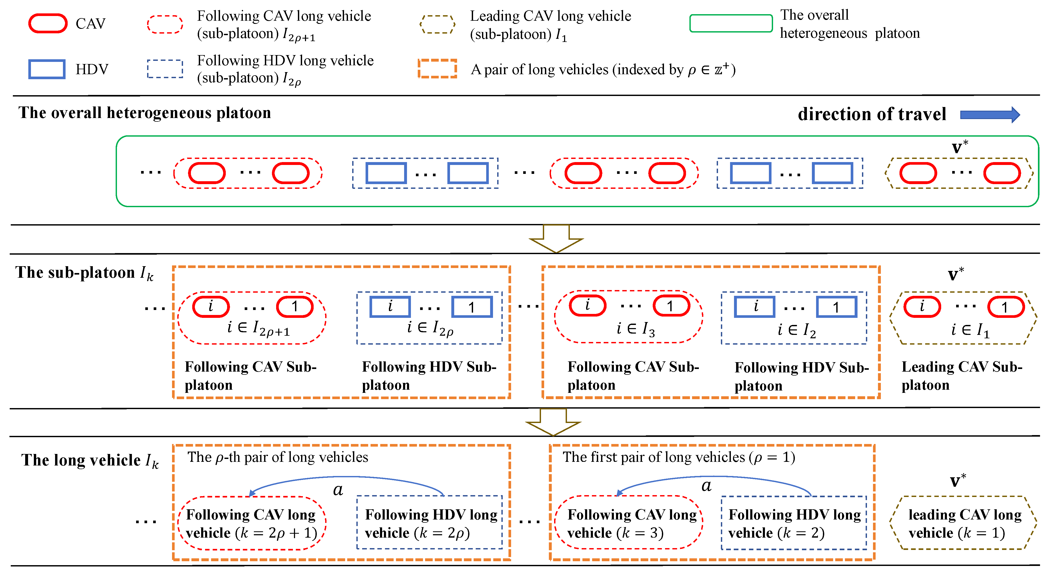
To incorporate the random CAV arrivals in the heterogeneous traffic flow, the stochastically heterogeneous traffic flow is designed as follows. The leading CAV sub-platoon and the first following HDV sub-platoon consist of one vehicle, i.e., $i=1$ for $i\in I_1,I_2$. For the other following vehicles from $I_3$ to the platoon tail, the Poisson distribution Pois($\lambda$) is adopted to generate stochastic vehicle sequences. The Poisson distribution parameter $\lambda$ is set as the expected number of CAVs in the platoon, i.e., $\lambda =5$ when the vehicle number is 10 under 50% penetration rate, and $\lambda =8$ when the vehicle number is 10 under 80% penetration rate. The CAV positions in the platoon are randomly selected in the Poisson-distributed stochastic vehicle sequence, and the other positions hold for HDVs.

Scenarios 1a and 1b are designed to demonstrate the controller performance with the stochastic sequence of CAV in the heterogeneous traffic flow at 50% CAV penetration rate considering communication delay of $\tau$ = 1 s and disturbances of HDVs. The leading CAVs in Scenarios 1a and 1b travel at the equilibrium velocity, while the following HDV sub-platoon $I_2$ is set to decelerate at −2 ${\mathrm{m}/\mathrm{s}}^2$ from 11 s to 15 s. Scenarios 2a and 2b aim to test controller performance under an increased communication delay of $\tau$ = 2 s, with other settings remaining unchanged. Scenarios 3a and 3b are designed to evaluate the controller performance under different HDV disturbances of increased magnitude and frequency, while other settings are the same as Scenarios 1a and 1b. In Scenarios 3a and 3b, the first HDV in the following HDV sub-platoon decelerates at −3 ${\mathrm{m}/\mathrm{s}}^2$ from 11 s to 15 s and then decelerates at −2 ${\mathrm{m}/\mathrm{s}}^2$ from 81 s to 85 s. Scenarios 4a and 4b intend to demonstrate the controller performance in higher CAV penetration rates of 80% and the other settings are the same as Scenarios 1a and 1b.

6.2. Simulation Results and Analysis

The generated trajectories of the proposed controller in Scenarios 1a to 4b are illustrated in Figure 3, Figure 4, Figure 5, Figure 6, Figure 7, Figure 8, Figure 9 and Figure 10, which demonstrate the platoon stability of the heterogeneous traffic flow. In these figures, the HDVs and CAVs are distinguished by the solid and dashed line styles. The red solid line represents the disturbed HDV, the solid orange lines represent the second HDV in $I_2$, and the gray solid lines represent the other HDVs. The blue dashed lines represent the CAVs except for the second CAV in $I_3$, which is represented by the green dashed lines. The legend shows the vehicle sequence within the heterogeneous platoon. The trajectories of the first CAV and the first HDV are pre-defined. The first CAV travels with the equilibrium velocity and the first HDV applies the HDV dynamics model with the pre-defined disturbance settings. The horizontal axis is time and the vertical coordinates in Figure 3a–c, Figure 4a–c, Figure 5a–c, Figure 6a–c, Figure 7a–c, Figure 8a–c, Figure 9a–c and Figure 10a–c indicate the velocity, acceleration, and spacing, respectively. The maximum and minimum values of fluctuations in velocity, acceleration, and spacing for the second HDV and the second CAV are labeled in orange and green, respectively.

In the following analysis, the velocity stabilization of the overall platoon is reached when the velocity differences of all vehicles are less than 0.05 m/s, and the acceleration stabilization is reached when the acceleration differences of all vehicles are less than 0.01 ${\mathrm{m}/\mathrm{s}}^2$. The time for velocity and acceleration stabilization are labeled as bold numbers on the horizontal axis of Figure 3a,b, Figure 4a,b, Figure 5a,b, Figure 6a,b, Figure 7a,b, Figure 8a,b, Figure 9a,b and Figure 10a,b.

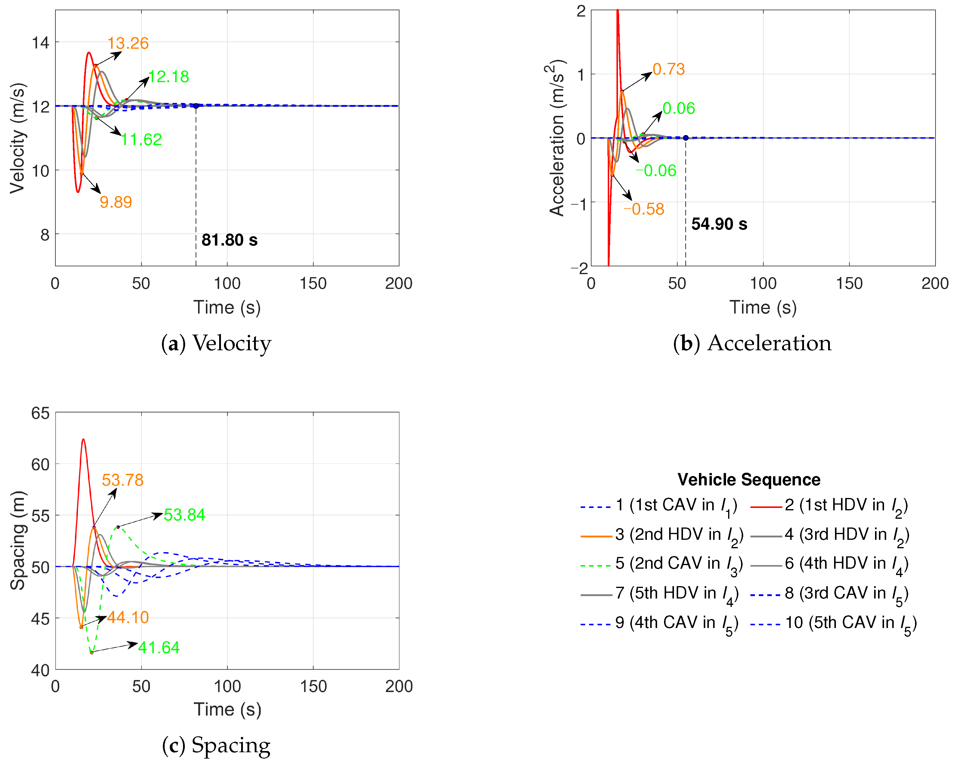
Scenarios 1a and 1b simulate the communication delay of $\tau$ = 1 s and the acceleration disturbance of −2 ${\mathrm{m}/\mathrm{s}}^2$ with 10 vehicles and 20 vehicles, respectively. The velocity, acceleration, and spacing trajectories in Scenarios 1a and 1b are illustrated in Figure 3 and Figure 4.In Scenario 1a, five sub-platoons are stochastically generated, i.e., one CAV, three HDVs, one CAV, two HDVs, and three CAVs in $I_1$ to $I_5$, respectively, as shown in the legend. The first HDV is set to decelerate with −2 ${\mathrm{m}/\mathrm{s}}^2$ from 11 s to 15 s, and later it starts to accelerate due to the car-following behavior of the HDV dynamics model. The acceleration fluctuations of the first HDV result in deviations of the following vehicles from the equilibrium velocity, acceleration, and spacing. The velocity fluctuations of the second HDV in $I_2$ and the second CAV in $I_3$ range from 9.89 m/s to 13.26 m/s and from 11.62 m/s to 12.18 m/s, respectively; see Figure 3a. In Figure 3b, the acceleration fluctuations of the second HDV in $I_2$ and the second CAV in $I_3$ range from −0.58 ${\mathrm{m}/\mathrm{s}}^2$ to 0.73 ${\mathrm{m}/\mathrm{s}}^2$ and from −0.06 ${\mathrm{m}/\mathrm{s}}^2$ to 0.06 ${\mathrm{m}/\mathrm{s}}^2$, respectively. The second CAV deviates less than the second HDV from the equilibrium velocity and acceleration, which demonstrates the CAV stability facing external disturbances. The velocity stabilization and acceleration stabilization are reached at 81.80 s and 54.90 s, respectively; see Figure 3a,b. It is convincing that the proposed controller can stabilize the heterogeneous traffic flow to the equilibrium velocity. In Figure 3c, the spacings of the second HDV and the second CAV range from 44.10 m to 53.78 m and from 41.64 m to 53.84 m. The minimal spacing gap between the second CAV and the vehicle in front (41.64 m) is reached with the velocity of 11.69 m/s, which satisfies the safety following constraint. Since the controlled CAVs do not simply follow the decelerating motions of the preceding vehicles while the HDVs just follow the preceding vehicle, the space gaps of the CAVs are sometimes larger than the HDVs when the preceding vehicles decelerate, comparing the spacing changes between the second CAV and the second HDV in Figure 3c.

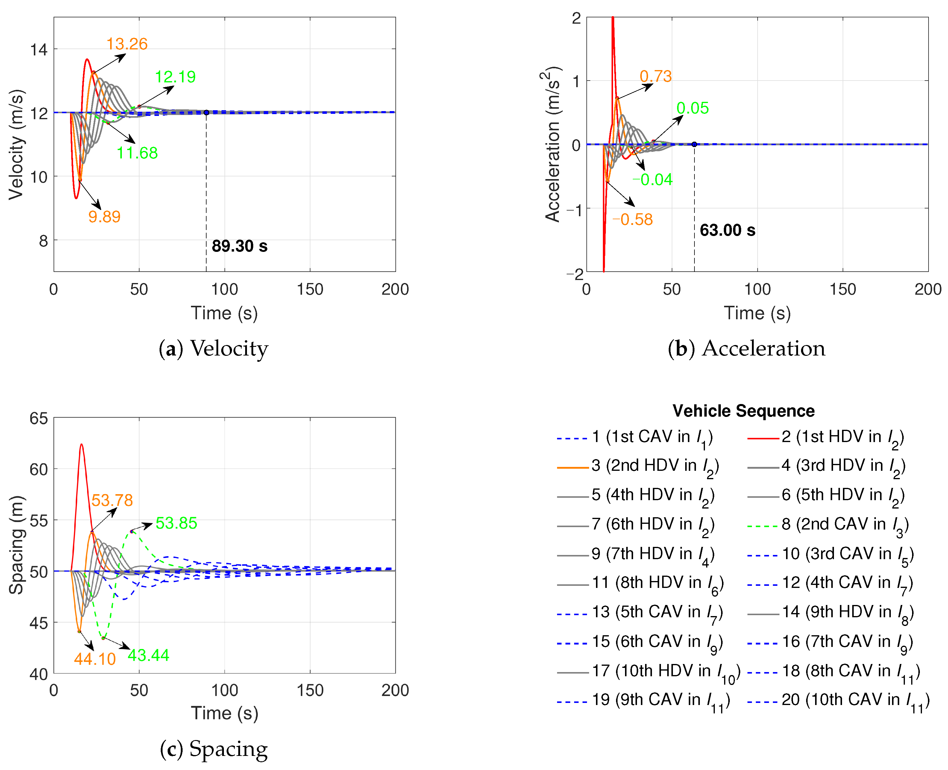
The heterogeneous platoon in Scenario 1b consists of eleven stochastically generated sub-platoons, i.e., one CAV, six HDVs, one CAV, one HDV, one CAV, one HDV, two CAVs, one HDV, two CAVs, one HDV, and three CAVs in $I_1$ to $I_{11}$, respectively, as shown in the legend of Figure 4. The magnitude of the communication delays and disturbances in Scenario 1b remains constant as in Scenario 1a, so the fluctuations of the second HDV in $I_2$ in velocity, acceleration, and spacing in Figure 4a–c are consistent with Scenario 1a in Figure 3a–c. The $I_2$ sub-platoon size changes in Scenarios 1a (three HDVs) and 1b (six HDVs), but the fluctuations in velocity, acceleration, and spacing of the second CAV in $I_3$ (see the green numbers) are slightly affected, comparing Figure 3a–c with Figure 4a–c. Moreover, the times for velocity and acceleration stabilization in Scenario 1b are 89.30 s and 63.00 s, respectively, which are larger than the counterparts in Scenario 1a; see Figure 4a–c. It can be concluded that the proposed control method can work in different platoon sizes, but an increase in platoon size leads to an increase in the time to stabilize the heterogeneous traffic flow.

Scenarios 2a and 2b are developed in a stochastic platoon sequence based on Scenarios 1a and 1b by increasing the communication delay $\tau$ from 1 s to 2 s. The velocity, acceleration, and spacing trajectories are illustrated in Figure 5 and Figure 6. Nine sub-platoons are stochastically generated in Scenario 2a, i.e., one CAV, one HDV, one CAV, two HDVs, one CAV, one HDV, one CAV, one HDV, and one CAV in $I_1$ to $I_9$, respectively, as shown in the legend. Figure 5a labels the maximal and minimal velocity fluctuations of the second CAV and the second HDV, which are quite close. In Figure 5b, the acceleration fluctuation of the second CAV is from −0.10 ${\mathrm{m}/\mathrm{s}}^2$ to 0.07 ${\mathrm{m}/\mathrm{s}}^2$ and the acceleration fluctuation of the second HDV is from −0.07 ${\mathrm{m}/\mathrm{s}}^2$ to 0.06 ${\mathrm{m}/\mathrm{s}}^2$. Comparing Scenario 2a with Scenario 1a, the second HDV follows the second CAV in Scenario 2a other than the first HDV in Scenario 1a, the velocity and acceleration fluctuation of the second HDV in Scenario 2a are much less than the counterpart in Scenario 1a. As shown in Figure 5a,b, the velocity and acceleration of the heterogeneous traffic flow are stable at 79.30 s and 52.00 s, respectively. The velocity and acceleration stabilization times in Scenario 2a are slightly different than Scenario 1a, which demonstrates the proposed controller is insensitive to an increase in the communication delay. The velocity and acceleration are stabilized faster in Scenario 2a compared with Scenario 1a since the disturbed HDV is followed by a CAV in Scenario 2a, which demonstrates the ability of CAVs to attenuate the disturbances and stabilize the traffic flow quickly. This observation verifies the CAVs can stabilize the traffic flow and reduce the adverse effects resulting from the disturbances on the following HDVs. The third CAV in $I_5$ essentially travels at equilibrium; thus, two CAVs are sufficient to stabilize the heterogeneous platoon. In Figure 5c, the spacing fluctuation of the second CAV is from 38.11 m to 53.77 and from 48.89 m to 50.47 m for the second HDV. The velocity is 11.86 m/s when the minimal spacing between the second CAV and the vehicle in front (38.11 m) is reached, which satisfies the safety constraint.

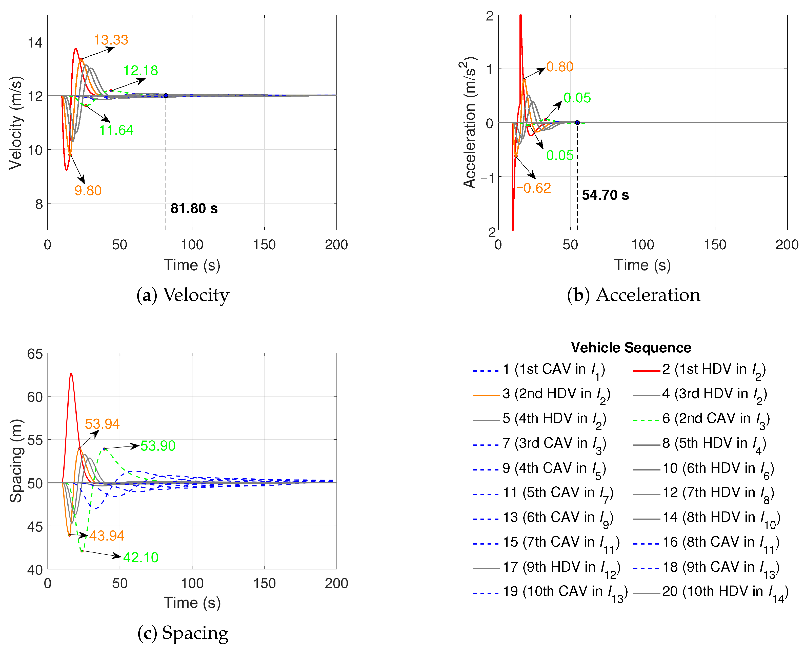
Scenario 2b generates 14 stochastic sub-platoons, i.e., one CAV, four HDVs, two CAVs, one HDV, one CAV, one HDV, one CAV, one HDV, one CAV, one HDV, two CAVs, one HDV, two CAVs, and one HDV in $I_1$ to $I_{14}$, respectively, as shown in the legend of Figure 6. Unlike Scenario 2a, three HDVs immediately follow the first HDV in Scenario 2b, and the disturbances are not diminished among these HDVs in $I_2$; see Figure 6a–c. However, the fluctuations in velocity and acceleration of the second controlled CAV in $I_3$ (see the green numbers) show slight variation compared with Scenario 2a, demonstrating the proposed control method can stabilize the heterogeneous traffic flow in different platoon sizes and configurations. The velocity stabilization and acceleration stabilization are reached at 81.80 s and 54.70 s, respectively. Compared with Scenario 2a, it is verified once again that a larger platoon size leads to a longer time to stabilize the heterogeneous traffic flow.

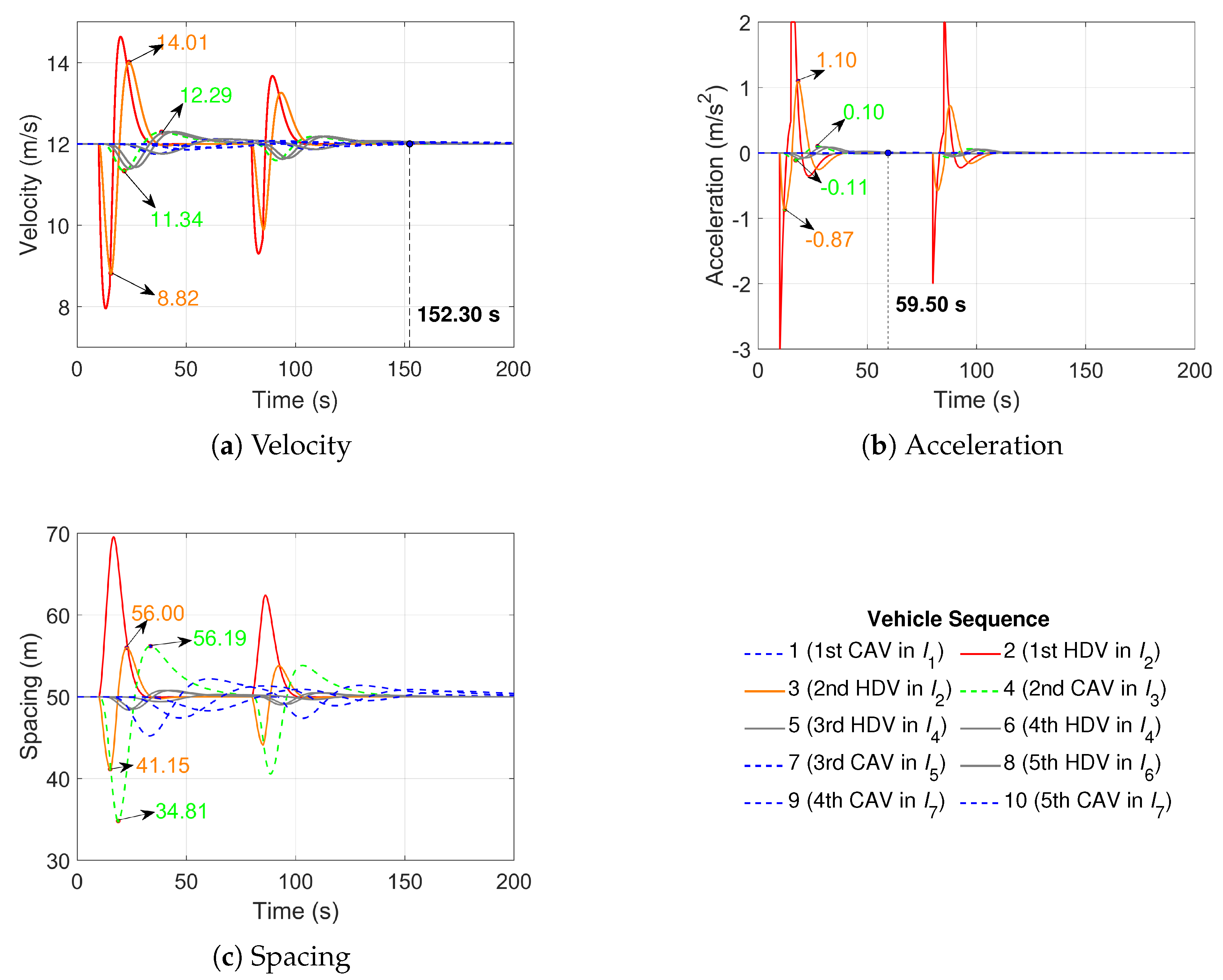
Scenarios 3a and 3b increase the disturbance frequency and amplitude from −2 ${\mathrm{m}/\mathrm{s}}^2$ to −3 ${\mathrm{m}/\mathrm{s}}^2$, and the velocity, acceleration, and spacing trajectories are illustrated in Figure 7 and Figure 8. Seven sub-platoons are stochastically generated in Scenario 3a, i.e., one CAV, two HDVs, one CAV, two HDVs, one CAV, one HDV, and two CAVs in $I_1$ to $I_7$, respectively, as shown in the legend. In Figure 7a, the velocity fluctuation of the second HDV is from 8.82 m/s to 14.01 m/s and for the second CAV it is from 11.34 m/s to 12.29 m/s. In Figure 7b, the acceleration fluctuation of the second HDV is from −0.87 ${\mathrm{m}/\mathrm{s}}^2$ to 1.10 ${\mathrm{m}/\mathrm{s}}^2$ and the acceleration fluctuation of the second CAV is from −0.11 ${\mathrm{m}/\mathrm{s}}^2$ to 0.10 ${\mathrm{m}/\mathrm{s}}^2$. In Figure 7c, the spacing fluctuation of the second HDV is from 41.15 m to 56.00 m. The spacing fluctuation of the second CAV is from 34.81 m to 56.19 m. The safety constraint is satisfied at the minimal spacing of 34.81 m with a velocity of 11.50 m/s. The velocity and acceleration stabilization times are 152.30 s and 59.50 s, respectively. The stabilization times are longer compared with Scenario 1a owing to the increased frequency and amplitude of the disturbances. Nevertheless, the heterogeneous traffic flow reaches equilibrium in Scenario 3a and the controller can effectively stabilize the heterogeneous traffic flow to the equilibrium velocity even if the disturbance frequency and amplitude are increased.

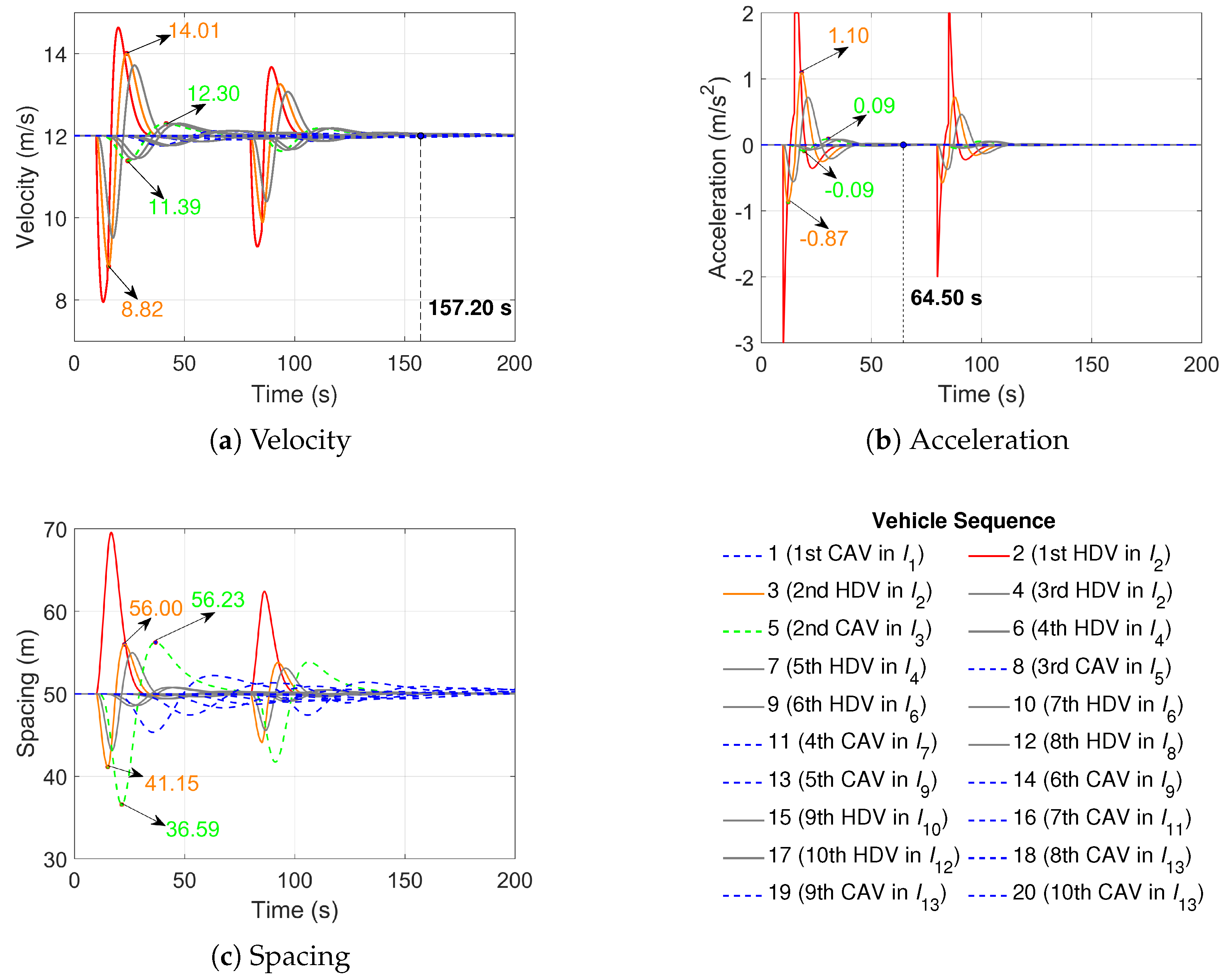
Scenario 3b generates 13 stochastic sub-platoons, i.e., 1 CAV, 3 HDVs, 1 CAV, 2 HDVs, 1 CAV, 2 HDVs, 1 CAV, 1 HDV, 2 CAVs, 1 HDV, 1 CAV, 1 HDV, and 3 CAVs in $I_1$ to $I_{13}$, respectively, as shown in the legend of Figure 8. Compared with Scenario 3a, the trajectories of the second HDV remain changed owing to the same vehicle sequence, whereas the trajectories of the second CAV change with small variations because of its varying vehicle sequence, as shown in Figure 8a,c. It can be verified the changes in the platoon size and vehicle sequence slightly affect the performance of the controlled CAVs. Furthermore, the velocity and acceleration stabilization times of the heterogeneous traffic flow in Figure 8a,b are longer than in Scenario 3a since the platoon size is enlarged in Scenario 3b.

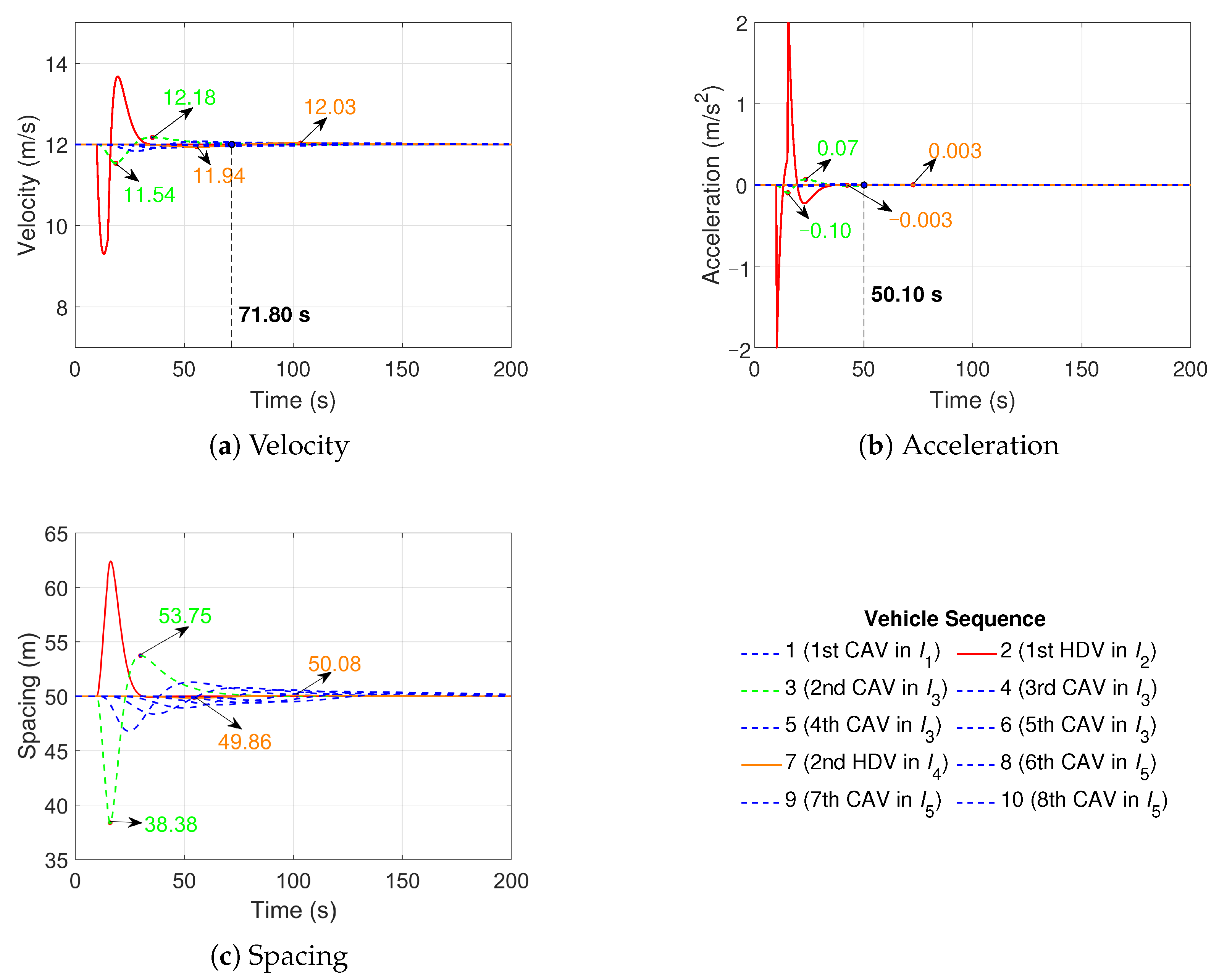
Scenarios 4a and 4b improve the CAV penetration rate to 80% based on Scenarios 1a and 1b, and the velocity, acceleration, and spacing trajectories are illustrated in Figure 9 and Figure 10. Five sub-platoons are stochastically generated in Scenario 4a, i.e., one CAV, one HDV, four CAVs, one HDV, and three CAVs in $I_1$ to $I_5$, respectively, as shown in the legend. In Figure 9a, the velocity of the second CAV fluctuates from 11.54 m/s to 12.18 m/s and the second HDV changes velocity from 11.94 m/s to 12.03 m/s. In Figure 9b, the acceleration fluctuation of the second CAV is from −0.10 ${\mathrm{m}/\mathrm{s}}^2$ to 0.07 ${\mathrm{m}/\mathrm{s}}^2$ and the acceleration of the second HDV is generally unchanged, from −0.003 to 0.003 ${\mathrm{m}/\mathrm{s}}^2$. We can see that the velocity and acceleration fluctuations of HDVs are reduced when the penetration rate of the CAVs increases. In Figure 9c, the spacing fluctuations of the second CAV and the second HDV are from 38.38 m to 53.75 m and from 49.86 m to 50.08 m, respectively. The minimal spacing gap of 38.38 m still satisfies the safety constraint with the instant velocity of 11.67 m/s. The velocity and acceleration stabilization times are 71.80 s and 50.10 s, respectively. The proposed controller in Scenario 4a can quickly stabilize the heterogeneous traffic flow in 80% CAV penetration rate compared with Scenario 1a of 50% CAV penetration rate.

Scenario 4b generates seven stochastic sub-platoons, i.e., one CAV, two HDVs, one CAV, one HDV, six CAVs, one HDV, and eight CAVs in $I_1$ to $I_7$, respectively, as shown in the legend of Figure 10. In Figure 10a–c, since the second HDV immediately follows the disturbed HDV, the velocity, acceleration, and spacing of the second HDV fluctuate significantly as the disturbed HDV does. The controlled CAVs are slightly affected by HDV disturbances; see the small fluctuations of the second CAV. The increased platoon size in Scenario 4b results in longer stabilization times for velocity and acceleration in the heterogeneous traffic flow. However, the differences in the stabilization times between Scenarios 4a and 4b are small due to the high penetration rate in Scenario 4b.

6.3. Comparison and Discussion

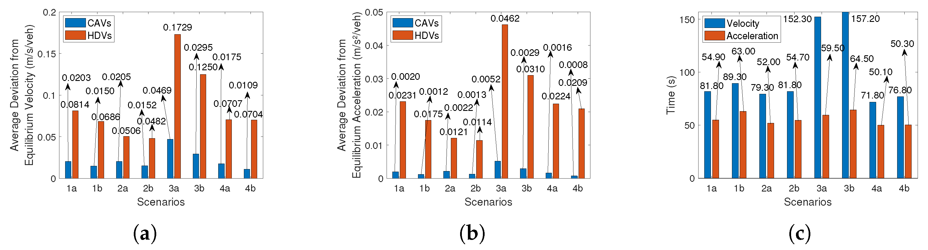
To further demonstrate the efficiency of the proposed controller, the deviations from the equilibrium velocity and acceleration for all CAVs and HDVs in Scenarios 1a to 4b are calculated, and the times for velocity and acceleration stabilization are listed for analysis; see Figure 11. The horizontal axis represents different scenarios, and the vertical axes in Figure 11a–c correspond to the average deviation from the equilibrium velocity, the average deviation from the equilibrium acceleration, and the times for velocity and acceleration stabilization, respectively.

Comparing Scenarios 1a to 2b, Scenarios 2a and 2b are conducted with an increased communication delay; thus, the average deviations from the equilibrium of the CAVs in Scenarios 2a and 2b are slightly greater than those in Scenarios 1a and 1b. This finding indicates that the proposed controller is insensitive to the communication delay. Scenarios 2a and 2b show fewer velocity and acceleration deviations from equilibrium for HDVs compared to Scenarios 1a and 1b, since the second CAV, which can stabilize the heterogeneous traffic flow, immediately follows the disturbed HDV. Comparing Scenario 1a with Scenario 2a, the times for velocity and acceleration stabilization in Scenario 2a are shorter than in Scenario 1a despite the increased communication delay in Scenario 2a. The same holds for Scenarios 1b and 2b. This observation demonstrates that the CAV sequence in the platoon matters and the CAVs can stabilize the heterogeneous traffic flow to be less affected by external disturbances. Since Scenarios 1b and 2b are conducted with a larger platoon size than Scenarios 1a and 2a, the times for velocity and acceleration stabilization in Scenarios 1b and 2b are longer, which illustrates that the increase in the platoon size positively affects the time for stabilization.

As shown in Figure 11, the deviations from equilibrium of the CAVs are significantly smaller than those of the HDVs in Scenarios 3a and 3b, which demonstrates the controlled CAVs can stabilize the traffic flow to equilibrium, while the HDVs just follow the preceding vehicles. Scenarios 3a and 3b are designed with an increased frequency and amplitude of the disturbance. Therefore, compared with Scenarios 1a to 1b, the average deviations from the equilibrium of the CAVs and the times for acceleration and velocity stabilization in Scenarios 3a and 3b are larger. Scenarios 1b and 3b are conducted with 20 vehicles, so the times for velocity and acceleration stabilization are longer compared with Scenarios 1a and 3a with 10 vehicles. As discussed in Scenarios 4a to 4b, the proposed controller is capable of stabilizing heterogeneous traffic flows at various CAV penetration rates. As shown in Figure 11, the times for velocity and acceleration stabilization decrease in Scenarios 4a to 4b compared with the other scenarios, which demonstrates the higher CAV penetration rates contribute to quicker stabilization of the heterogeneous traffic flow.

Overall, the controller performance in all scenarios verifies the proposed controller is insensitive to different ranges of communication delays and disturbances and is effective in stabilizing the heterogeneous traffic flow and attenuating the disturbance in the presence of different platoon sizes, communication delays, disturbances, and CAV penetration rates. The simulation results coincide with the intuition that CAVs can effectively stabilize disturbances in the heterogeneous traffic flow and reach the desired velocity and acceleration, while the HDVs just follow the preceding vehicles. The deviations from the equilibrium of the CAVs are less than the deviations of the HDVs in all scenarios. The increased platoon size lengthens the time for velocity and acceleration stabilization of the overall heterogeneous traffic flow but does not impact the controller performance. The changes in the vehicle sequence influence the stabilization time and the deviations from the equilibrium but rarely affect the performance of the controlled CAVs. The higher CAV penetration rates contribute to quicker stabilization of the heterogeneous traffic flow.

To further validate the effectiveness of the proposed method, comparative experiments are designed where CAVs are controlled using the IDM [34] and LQR [35], respectively. The comparative experiments are conducted using the same settings as Scenario 1a, including vehicle number, delay, and disturbance settings, apart from the difference in 20% CAV penetration rate and the platoon sequence (four sub-platoons of one CAV, one HDV, one CAV, and seven HDVs in $I_1$ to $I_4$). The heterogeneous platoon trajectories using different approaches are demonstrated in Figure 12, which verifies that the proposed control method has a significant effect on stabilizing the traffic flow compared to IDM and LQR. 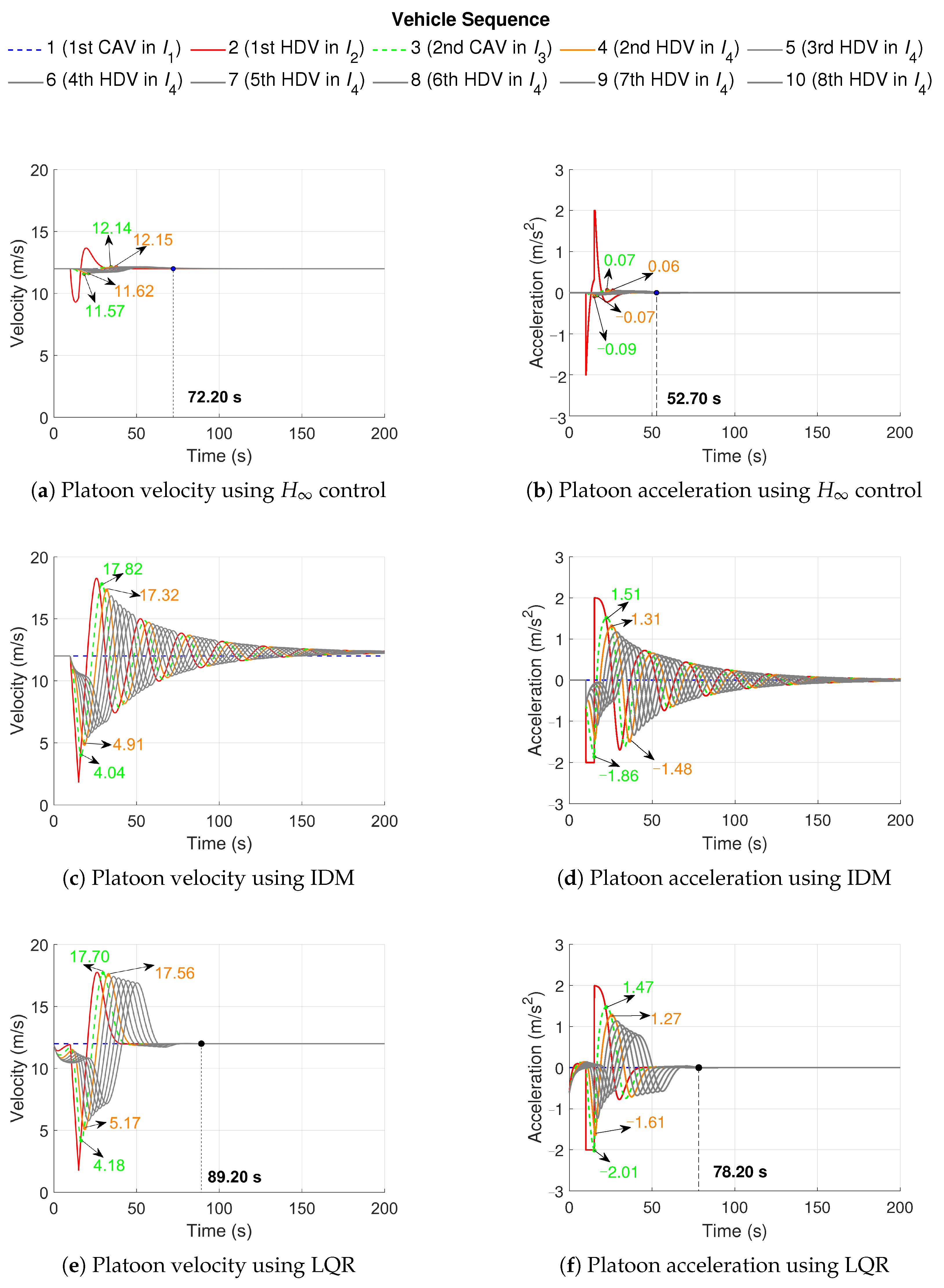Figure 12a,b show the platoon acceleration and platoon velocity using the proposed $H_{\infty }$ control method. The acceleration and velocity of the controlled CAV in $I_3$ fluctuates in a small range from 11.57 to 12.14 m/s and from −0.09 to 0.07 ${\mathrm{m}/\mathrm{s}}^2$, respectively. The second HDV in $I_4$ exhibits smaller fluctuations in velocity and acceleration, from 11.62 to 12.15 m/s and from −0.07 to 0.06 ${\mathrm{m}/\mathrm{s}}^2$, respectively. The velocity and acceleration of the overall platoon converge within 72.20 s and 52.70 s, which demonstrates the ability of the proposed $H_{\infty }$ control method to suppress the disturbances.

The platoon acceleration and platoon velocity using the IDM are presented in Figure 12c,d. The acceleration and velocity fluctuations of the CAV increase significantly subject to the first perturbed HDV in $I_2$, ranging from 4.04 to 17.82 m/s and −1.86 to 1.51 ${\mathrm{m}/\mathrm{s}}^2$, respectively. The second HDV exhibited significant velocity and acceleration fluctuations due to the inability of CAV to suppress the disturbance using the IDM, from 4.91 to 17.32 m/s and −1.48 to 1.31 ${\mathrm{m}/\mathrm{s}}^2$, respectively. The velocity and acceleration of the entire platoon using IDM are unable to converge, as the IDM cannot effectively stabilize perturbations in the traffic flow. Figure 12e,f show the platoon acceleration and platoon velocity using the LQR. The velocity and acceleration fluctuations of the controlled CAV are relatively significant, from 4.18 to 17.70 m/s and from −2.01 to 1.47 ${\mathrm{m}/\mathrm{s}}^2$, respectively. The second HDV also shows significant fluctuations in velocity and acceleration, from 5.17 to 17.56 m/s and −1.61 to 1.27 ${\mathrm{m}/\mathrm{s}}^2$. The velocity and acceleration of the platoon converge within 89.20 s and 78.20 s, respectively, demonstrating the ability of the LQR controller to suppress the propagation of disturbances. However, the convergence time is longer compared with the proposed $H_{\infty }$ control method, as in Figure 12a,b, which verifies the robustness and effectiveness of the proposed control method.

7. Conclusions and Future Work

In this paper, a robust $H_{\infty }$ controller for the stochastically heterogeneous traffic flow is proposed, taking the communication delay and the disturbances of the HDVs into account. To study the stochastic nature of heterogeneous vehicle arrivals, the proposed controller simplifies the stochastically heterogeneous traffic flow into multiple control problems of long vehicles (i.e., sub-platoons). For a pair of a CAV long vehicle and an HDV long vehicle, the time-lagged system is formulated and then the closed-loop system is derived, both of which treat the acceleration fluctuations of HDVs as disturbances. The stability of the closed-loop system is demonstrated using the $H_{\infty }$ norm of the closed-loop transfer function. Based on the time-lagged bounded real lemma, we derive a $H_{\infty }$ state feedback controller and demonstrate the stability of the heterogeneous platoon. The controller performance is verified by simulation of eight scenarios, considering various settings of platoon sizes, communication delays, disturbances, and CAV penetration rates. The results demonstrate the ability of the proposed controller to effectively stabilize the heterogeneous traffic flow for desired trajectories in all scenarios and the insensitivity to different communication delays and disturbances. Compared to IDM and LQR, the proposed controller shows better robustness and effectiveness in stabilizing the heterogeneous traffic flow. The controlled CAVs deviate from equilibrium less than the HDVs that follow the preceding vehicles. The higher CAV penetration rates and the early CAV arrivals can quickly stabilize the heterogeneous traffic flow.

Future research will incorporate the lane-changing behaviors on a multi-lane expressway or on- and off-ramp, taking into account packet loss and parameter uncertainties. The new incoming vehicles after detection will be immediately controlled in a real-time event-based algorithm to stabilize the heterogeneous traffic flow. Moreover, sensor noise will be explicitly incorporated into the system model to validate the robustness of the control strategy under realistic measurement conditions.