Backstepping Command Filter Control for Electromechanical Servo Systems with Unknown Dynamics Based on Reinforcement Learning

Abstract

To address the challenges of acquiring precise dynamic models for electromechanical servo systems and the susceptibility of system state information to noise, a backstepping command filter controller based on reinforcement learning is proposed. This method can achieve high-precision and low-energy control in electromechanical servo systems subject to noise interference and unmodeled disturbances. The proposed method employs a command filter to obtain differential estimations of known signals and process noise. Reinforcement learning is employed to estimate unknown system disturbances, including unmodeled friction and external interference. The weights of the networks are updated using an online gradient descent algorithm, eliminating the need for an offline learning phase. In addition, the Lyapunov function analysis method is used to demonstrate the stability of the closed-loop system. To validate the effectiveness of the proposed method, comparative experiments were conducted using an electromechanical servo experimental platform. The experimental results indicate that, compared to other mainstream controllers, the control algorithm excels in tracking accuracy, response speed, and energy efficiency, and demonstrates significant robustness against system uncertainties and external disturbances.

1. Introduction

In recent years, the tracking control problem of electromechanical servo systems has garnered significant attention in both theoretical research and practical applications, owing to their inherent uncertainties [1,2,3,4]. Servo systems are widely used in high-precision fields, such as autonomous driving, unmanned aerial vehicle (UAV) navigation, and robotic control. However, the complex dynamic characteristics and uncertainties of these systems pose substantial challenges for achieving precise control. Inadequate handling of uncertainties and external disturbances can lead to deviations from the desired trajectory or even system instability, thereby compromising both the performance and safety. To address these issues, various control strategies have been proposed, including adaptive robust control, sliding mode control (SMC), and disturbance rejection control [5,6,7,8]. However, these methods often rely on partial or full knowledge of system dynamics, limiting their applicability in scenarios where the dynamic parameters are entirely unknown, particularly in industrial and engineering contexts where practical constraints are significant.

Model-free control strategies have gained considerable interest in overcoming reliance on dynamic models. These approaches, including iterative learning control [9], neural network control [10], reinforcement learning (RL) control [11], and optimal control [12], reduce dependence on precise system models and expand the scope of control technologies. However, they still face challenges in managing uncertainties, external disturbances, and noise in complex dynamic environments where maintaining stable control remains difficult.

To cope with these complex environments, researchers have explored the potential of combining RL with classical control methods [13,14,15]. The combination of RL’s adaptability and the stability of classical control techniques can effectively overcome the limitations of traditional methods in dynamic environments.

A previous study [16] introduced a hybrid control strategy based on the actor-critic architecture, enabling the simultaneous estimation of multiple PID controller gains. This strategy does not rely on precise dynamic models and can adaptively adjust to dynamic behaviors and operating environments, although its theoretical stability proof remains incomplete. Other studies [17,18] employed Lyapunov methods to verify RL stability in complex systems, such as helicopters and robots, but found it to be less effective in handling external disturbances. In practical applications, servo systems often encounter uncertain disturbances that can significantly degrade control performance or even lead to instability [19,20].

To enhance disturbance rejection, some studies have combined RL with disturbance observers. For example, refs. [21,22] proposed integrating RL with fuzzy logic systems (FLS). In [21], RL optimizes the virtual and actual control at each step of the backstepping control, whereas FLS approximates unknown functions and provides feedforward compensation. Similarly, ref. [22] applied the FLS to approximate unknown functions in large-scale nonlinear systems by utilizing state observers to estimate unmeasured states. However, the performance of an FLS is highly dependent on fuzzy rule design, which often requires extensive experimental tuning, complicating practical implementation. In addition, ref. [23] proposed combining RL with sliding mode control, offering a solution distinct from traditional integral sliding mode control. This sliding mode controller uses neural networks for approximation and disturbance estimation, while an actor-critic architecture continuously learns the optimal control strategy using adaptive dynamic programming (ADP). However, the inherent discontinuity in sliding mode control may lead to chattering, which negatively impacts performance. Another study [24] integrated RL with the robust integral of the sign of the error (RISE) controller using an actor-critic architecture to approximate unknown dynamics for feedforward compensation. While this improved the control accuracy, the high sensitivity of the sign function to error variations weakened the robustness of the system to noise. In environments with significant measurement noise, the RISE controller may misinterpret the noise as an error, exacerbating fluctuations in the control inputs. Despite these advancements, further research is necessary to develop more flexible and precise control strategies for handling greater uncertainties and complex environments.

This study proposes a novel backstepping command filter controller based on reinforcement learning (BCF-RL) to address these challenges. The BCF-RL controller effectively tackles the challenge of obtaining accurate dynamic models and reduces sensitivity to noise in state measurements. Using an actor-critic framework, the adaptive RL control strategy estimates unknown disturbances in real time and provides feedforward compensation, significantly mitigating the impact of unmodeled dynamics and external perturbations. Traditional noise suppression methods, such as the extended Kalman filter (EKF) and low-pass filters, are effective and often face high computational complexity and reduced robustness in nonlinear systems. By avoiding excessive signal smoothing, command filters achieve better noise suppression and faster response times, making them a more suitable choice.

Compared with the method in [16], the BCF-RL approach provides more rigorous theoretical stability guarantees. Unlike traditional sliding mode control, it reduces chattering and improves system performance. Furthermore, compared with the RISE control strategy in [24], this method demonstrates greater robustness to sensor noise while achieving faster response times. One key advantage is its minimal reliance on prior system knowledge, which allows for asymptotic tracking and robust performance against both unknown dynamics and external disturbances. These features make the BCF-RL a promising solution for the precise control of complex dynamic systems with high uncertainty. The contributions of this study are as follows:

(1)

Given the sensitivity of the system speed signal to the measurement noise, a command filter was developed to process this noise, thereby enhancing the robustness of the controller.

(2)

A hybrid data-model-driven control method was designed. By employing the actor-critic structure of reinforcement learning, this method provides a more accurate estimation of unknown disturbances, resulting in a higher accuracy in position tracking.

(3)

The stability of the controller in reinforcement learning and the weight convergence of the two networks are rigorously proven from a theoretical perspective, ensuring the robustness and effectiveness of the control strategy.

This article is organized as follows: Section 2 introduces the problem formulation and system architecture. Section 3 details the design process of the main controller. Section 4 describes the design process of the auxiliary controller. Section 5 provides stability analysis and proof. Section 6 presents the experimental results. Finally, Section 7 concludes the article.

2. Problem Formulation and System Architecture

2.1. Description of Servo System

The servo system depicted in Figure 1 is a positioning system in which the inertial load is directly driven by a permanent magnet synchronous motor (PMSM). The control objective is to ensure that the inertial load closely follows a specified smooth motion trajectory $x_d$. Typically, the bandwidth of the motor current loop is much greater than that of the velocity and position loops, allowing the current dynamics to be neglected. The dynamic characteristics of the servo system are described by (1).

$$k_{u}u=M\ddot{\theta }+T_f+f(t)$$

(1)

In (1), $\theta$, $\dot{\theta }$ and $\ddot{\theta }$ represent angular displacement, angular velocity, and angular acceleration, respectively. $k_u$ is the torque constant, u is the control signal, $M$ denotes the inertial load coefficient. The term $f\left(t\right)$ accounts for other unmodeled disturbances such as nonlinear friction, external disturbances, and unmodeled dynamics. $T_f$ is represented by the nonlinear friction model as follows:

$$T_f(\dot{\theta })=a_1\dot{\theta }+a_2\tanh (c_1\dot{\theta })+a_3[\tanh (c_2\dot{\theta })-\tanh (c_3\dot{\theta })]$$

(2)

where $a_1,a_2,a_3$ represent the amplitude levels of different friction characteristics, $c_1,c_2,c_3$ are the shape coefficients characterizing different friction characteristics. $a_1\dot{\theta }$ characterizes the viscous friction torque, $a_2\mathrm{t}\mathrm{a}\mathrm{n}\mathrm{h}\left(c_1\dot{\theta }\right)$ characterizes the Coulomb friction characteristics, $a_3[\mathrm{t}\mathrm{a}\mathrm{n}\mathrm{h}(c_2\dot{\theta }$)$- \mathrm{t}\mathrm{a}\mathrm{n}\mathrm{h}(c_3\dot{\theta }$)] characterizes the Stribeck effect.

Considering sensor measurement errors, the dynamics equation can be modified to include an additional error term $n$. Defining ${\left[x_1,x_2\right]}^T={\left[\theta ,\dot{\theta }\right]}^T$, the state equation of the system is as follows:

$$\begin{array}{l}{\dot{x}}_1=x_2+n\\ {\dot{x}}_2=Ku-\beta \phi (x_2)-F(t)\end{array}$$

(3)

where $K=k_u/M$ is the control coefficient. $\beta ={a_1,a_2,a_3]}^T\phi \left(x_2\right)=[a_1\dot{\theta },a_2\tanh \left(c_1\dot{\theta }\right), a_3[\mathrm{t}\mathrm{a}\mathrm{n}\mathrm{h}(c_2\dot{\theta }$)$- \mathrm{t}\mathrm{a}\mathrm{n}\mathrm{h}(c_3\dot{\theta }$)], $\beta \phi \left(x_2\right)$ is viscous friction and $F\left(t\right)=f\left(t\right)/M$ represents unknown disturbances. It is worth noting that the controller designed in this study relies only on the known control coefficient $K$, measurable angular displacement $x_1$, and angular velocity $x_2$.

2.2. Design of Control System Architecture

The design objective of the controller is to obtain u such that $x_1$ of the inertial load can track the desired trajectory $x_d$ while ensuring that the system signals remain bounded. The following assumptions were made to facilitate the controller design process.

Assumptions. 

(1)

The desired reference trajectory $x_d$ and its first derivative are both existent and bounded.

(2)

The measurement noise n and the unknown interference $f\left(t\right)$ are bounded, with known upper and lower limits.

3. Design of BCF Main Controller

3.1. Design of Differential Command Filter

In practical systems, the direct differentiation of real-time signals can amplify the noise and cause numerical instability. Therefore, it is essential to design differential-command filters to mitigate these issues.

Lemma 1. 

Define a command filter as specified in (4).

$$\dot{\widehat{\rho }}(t)=-{\lambda }_e(\widehat{\rho }(t)-\rho (t))$$

(4)

where ${\lambda }_e>0$ is the constant gain, $\widehat{\rho }\left(t\right)$ is the intermediate state of the command filter, $\rho \left(t\right)$ is the input of the filter, $\dot{\widehat{\rho }}\left(t\right)$ is the output of the filter, and $\widehat{\rho }\left(0\right)=\rho \left(0\right)$ is the initial state of the filter. If $\rho \left(t\right)$ is continuous, $\rho \left(t\right),\dot{\rho }\left(t\right)\in \Omega$ ($\Omega$ is a compact set), and $\rho \left(0\right),\dot{\rho }\left(0\right),\widehat{\rho }\left(0\right)$ is bounded, both $\dot{\rho }-\dot{\widehat{\rho }}$ is bounded.

Proof of Lemma 1. 

Define $\epsilon =\widehat{\rho }-\rho$. According to (4), the first derivative of $\epsilon$ can be expressed as shown in (5).

$$\dot{\epsilon }=\dot{\widehat{\rho }}-\dot{\rho }=-{\lambda }_e\epsilon -\dot{\rho }$$

(5)

Because $\epsilon \left(0\right)=\widehat{\rho }\left(0\right)-\rho \left(0\right)=0$, according to ref. [25], it can be concluded that (6) is old.

$$\left|\epsilon (t)\right|=\left|{\displaystyle {\int }_0^t\dot{\rho }(s)\exp \left(-{\lambda }_e(t-s)\right)\mathrm{d}s}\right|\le {\displaystyle \frac{\eta }{{\lambda }_e}}$$

(6)

where $\eta ={max}_{\dot{e\in \mathsf{\Omega }}}\left|\dot{\rho }\right|$.

Define $\varsigma =\dot{\widehat{\rho }}-\dot{\rho }$. ${\varsigma }_m=max\left|\varsigma \right|$. Based on $\left|\dot{\widehat{\rho }}\right|=\left|-{\lambda }_e\epsilon \right|\le \eta$, and according to (5) and (6), it can be obtained as shown in (7):

$$\left|\varsigma \right|=\left|\dot{\widehat{\rho }}-\dot{\rho }\right|\le \left|\dot{\widehat{\rho }}\right|+\left|\dot{\rho }\right|=2\eta \le {\varsigma }_m$$

(7)

□

3.2. Design of Dummy Control Law α

The feedback inputs to the BCF main controller are states $x_1$ and $x_2$, and the output is the control law u. The design of the BCF controller primarily includes the differential command filter, dummy control law α for $x_2$, and actual control law $u$.

$e_1$ and $e_2$ are defined in (8).

$$\begin{array}{l}{e}_1=x_1-x_d\\ e_2=x_2-\alpha \end{array}$$

(8)

For tracking error $e_1$ to approach zero, it is necessary to ensure that its derivative approaches zero. By differentiating $e_1$, we obtain Equation (8).

$${\dot{e}}_1={\dot{x}}_1-{\dot{x}}_d=x_2+n-{\dot{x}}_d$$

(9)

To ensure the convergence of $e_1$, a Lyapunov function $V_1$ is designed as $V_1=0.5e_1^2$.

According to (8) and (9), the derivative of $V_1$ can be obtained, as shown in (10).

$${\dot{V}}_1=e_1{\dot{e}}_1=e_1\left(\alpha +e_2+n-{\dot{x}}_d\right)$$

(10)

Because of the unknown measurement noise, n, an analytical expression for ${\dot{V}}_1$ cannot be obtained. Based on Lemma 1, the command filter is constructed, as shown in (11).

$${\dot{e}}_1={\dot{\widehat{e}}}_1+{\varsigma }_1=-{\lambda }_{e1}({\widehat{e}}_1-e_1)+{\varsigma }_1$$

(11)

where ${\varsigma }_1={\dot{\widehat{e}}}_1-{\dot{e}}_1$.

By substituting (11) into (9), the expression for n can be derived as shown in (12).

$$n={\dot{\widehat{e}}}_1+{\varsigma }_1-x_2+{\dot{x}}_d$$

(12)

By substituting (12) into (10), Equation (13) can be obtained:

$${\dot{V}}_1=e_1\left(\alpha +e_2+{\dot{\widehat{e}}}_1+{\varsigma }_1-x_2\right)$$

(13)

Therefore, the dummy control law $\alpha$ can be designed as shown in (14).

$$\alpha =x_2-{\dot{\widehat{e}}}_1-k_1{e}_1$$

(14)

where $k_1>0$ is the control gain.

3.3. Design of Actual Control Law u

In Equation (8), to ensure the convergence of the dummy control error $e_2$, it is necessary for its derivative to approach zero. Consequently, Equation (15) can be derived.

$${\dot{e}}_2=Ku-\beta \phi (x_2)-F(t)-\dot{\alpha }$$

(15)

To ensure the convergence of $e_2$, a Lyapunov function $V_2$ is designed, as shown in (16).

$$V_2={\displaystyle \frac{1}{2}}{e}_2^2$$

(16)

The derivative of $V_2$ can be expressed as shown in (17).

$${\dot{V}}_2=e_2(Ku-\beta \phi (x_2)-F(t)-\dot{\alpha })$$

(17)

Unknown nonlinear $\dot{\alpha }$ can be constructed by command filter as (18).

$$\dot{\alpha }=\dot{\widehat{\alpha }}+{\varsigma }_2=-{\lambda }_{e2}(\widehat{\alpha }-\alpha )+{\varsigma }_2$$

(18)

where ${\varsigma }_2={\dot{\widehat{e}}}_2-{\dot{e}}_2$.

The unknown disturbance F is estimated using the RL auxiliary controller, and the estimated result is $\widehat{F}=F+\tilde{F}$. $\tilde{F}$ represents the estimation error, which is further detailed in Section 4.

Therefore, the actual control law u can be designed as shown in (19).

$$u=-(-\widehat{F}-\dot{\widehat{\alpha }}-\beta \phi (x_2)+e_1+k_2{e}_2)/K$$

(19)

where $k_2>0$ is the control gain.

Substituting (19) into (15) yields the expression for the estimation error, as shown in Equation (20).

$$\tilde{F}={\dot{e}}_2-e_1-k_2{e}_2-{\varsigma }_2$$

(20)

3.4. Controller Overall Architecture

The BCF-RL controller was designed to address technical challenges in electromechanical servo systems. It consists of a BCF main controller and an RL auxiliary controller. The BCF main controller integrates a command filter into the backstepping control, enhancing the system’s response speed and significantly reducing errors caused by measurement noise. This improves the robustness and accuracy of the system. The RL auxiliary controller handles the online estimation of unknown disturbances in the system. Utilizing critic and actor neural networks, the RL auxiliary controller adapts to dynamic changes and effectively estimates the complex nonlinear disturbances. This combination enhances the adaptive capability of the system and improves the stability and reliability of the controller for practical applications. The controller structure is illustrated in Figure 2.

4. Design of RL Auxiliary Controller

The RL auxiliary controller, which includes an actor neural network and a critic neural network, is an efficient approach for solving the optimal control problems for nonlinear systems. The core of this method lies in the actor network’s ability to achieve timely feed-forward compensation by dynamically estimating uncertainty disturbances in a nonlinear system. Concurrently, the critic network evaluates the operating cost in real time, quantifies the performance of the current control strategy, and provides feedback to the actor network to optimize its subsequent decision-making process. The design of the RL auxiliary controller is described in this section.

4.1. Preliminaries

To achieve optimal tracking control, the instantaneous cost function is defined as (21).

$$r(t)={\tau }_1{e}_1^2(t)+{\tau }_2{u}^2(t)$$

(21)

where ${\tau }_1>0$ and ${\tau }_2>0$ are constant coefficients. To achieve optimal tracking control, the infinite time-domain cost function J to be minimized is represented by (22).

$$J(t)={\displaystyle {\int }_t^{\infty }{e}^{-\gamma (s-t)}}r(s)ds$$

(22)

where γ represents the discount factor, which ensures that the cost function $J$ is bounded even if the ideal trajectory does not approach 0. By transforming the above equation, the following Bellman equation is obtained as (23).

$$\gamma J(t)=r(t)+\dot{J}(t)$$

(23)

4.2. Critic Neural Network

A critic neural network is used to approximate the value function of the Bellman equation in reinforcement learning. In this study, the critic network generated a scalar evaluation signal that is then used to tune the actor network. Based on the general approximation properties of neural networks, cost function J can be expressed (24).

$$J(x_c)=W_c^{T}g\left(V_c^T{x}_c\right)+{\epsilon }_c$$

(24)

The input of the critic neural network is ${\mathit{x}}_c={\left[x_1{x}_2{e}_1{e}_{2}u\right]}^T$. ${\mathit{V}}_c$ is the weight value from the input layer to the hidden layer of the critic network, ${\mathit{W}}_c$ is the weight value from the hidden layer to the output layer, ${\epsilon }_c$ is the reconstruction error of the neural network, and $g\left(·\right)$ represents $tanh\left(·\right)$. Therefore, the approximate value of J can be expressed (25).

$$\widehat{J}(x_c)={\widehat{W}}_c^{T}g\left({\widehat{V}}_c^T{x}_c\right)$$

(25)

where ${\widehat{\mathit{W}}}_c$ is the estimated value of ${\mathit{W}}_c$ and ${\widehat{\mathit{V}}}_c$ is the estimated value of ${\mathit{V}}_c$. The mismatch between the estimated and ideal weights is defined as ${\tilde{\mathit{W}}}_c={\widehat{\mathit{W}}}_c-{\mathit{W}}_c$ and ${\tilde{\mathit{V}}}_c={\widehat{\mathit{V}}}_c-{\mathit{V}}_c$, respectively.

Taking the derivative of $\widehat{J}$ yields (26).

$$\begin{array}{c}\dot{\widehat{J}}(x_c)={\dot{\widehat{W}}}_c^{T}g\left({\widehat{V}}_c^T{x}_c\right)+{\widehat{W}}_c^T\left(\nabla g_c\odot \left({\widehat{V}}_c^T{\dot{x}}_c\right)\right)\\ +{\widehat{W}}_c^T\left(\nabla g_c\odot \left({\dot{\widehat{V}}}_c^T{x}_c\right)\right)\end{array}$$

(26)

where $\nabla g_c=0.5\left(1-g_c{⨀g}_c\right)$, ${\mathit{X}}_c={\widehat{\mathit{V}}}_c^T{\mathit{x}}_c,g_c=g\left({\mathit{X}}_c\right)$, and $\odot$ represent the matrix multiplication by bit (Hadamard product). In the design of the neural network weights, only ${\widehat{\mathit{W}}}_c^T\left(\nabla g_c\odot \left({\widehat{\mathit{V}}}_c^T{\dot{\mathit{x}}}_c\right)\right)$ was considered.

The prediction error was defined as $e_c=r\left(t\right)+\dot{\widehat{J}}\left(t\right)-\gamma \widehat{J}\left(t\right)$. The objective function minimizes the approximation error in (27).

$$E_c={\displaystyle \frac{1}{2}}{e}_c^2$$

(27)

Taking the partial derivative of $E_c$ over ${\mathit{W}}_c$ yields (28).

$${\displaystyle \frac{\partial E_c}{\partial {\widehat{W}}_c}}={\displaystyle \frac{\partial E_c}{\partial e_c}}{\displaystyle \frac{\partial e_c}{\partial {\widehat{W}}_c}}=e_c({\displaystyle \frac{\partial (\dot{\widehat{J}}(t)-\gamma \widehat{J}(t))}{\partial {\widehat{W}}_c}})=-\gamma e_c{g}_c+e_c\nabla g_c\odot ({\widehat{V}}_c^T{\dot{x}}_c)$$

(28)

Therefore, the updating law of ${\mathit{W}}_c$ can be designed as (29).

$$\begin{array}{cc}\hfill {{\displaystyle \dot{\widehat{W}}}}_c& =-l_{c1}{\displaystyle \frac{\partial E_c}{\partial {\widehat{W}}_c}}-l_{c2}{\widehat{W}}_c=-l_{c1}{e}_c(-\gamma g_c)-l_{c2}{\widehat{W}}_c\hfill \\ & =-l_{c1}\left(r+\dot{\widehat{J}}(t)-\gamma \widehat{J}\right)(-\gamma g_c)-l_{c2}{\widehat{W}}_c\hfill \\ & =-l_{c1}\left(r+{\widehat{W}}_c^T(-\gamma g+\nabla g_c\odot X_c)\right)(-\gamma g_c)-l_{c2}{\widehat{W}}_c\hfill \\ & =-l_{c1}\left(r+{\widehat{W}}_c^T\Lambda \right)(-\gamma g_c)-l_{c2}{\widehat{W}}_c\hfill \end{array}$$

(29)

where $\mathsf{\Lambda }=\nabla g_c\odot {\mathit{X}}_c-\gamma g_c$, $l_{c1}>0,l_{c2}>0$ were used to adjust the convergence rate of the weight values.

Taking the partial derivative of E_c over ${\mathit{V}}_c$ yields (30).

$$\begin{array}{cc}\hfill {\displaystyle \frac{\partial E_c}{\partial {\widehat{V}}_c}}& ={\displaystyle \frac{\partial E_c}{\partial e_c}}{\displaystyle \frac{\partial e_c}{\partial {\widehat{V}}_c}}=e_c(-\gamma {\displaystyle \frac{\partial \widehat{J}}{\partial {\widehat{V}}_c}})\hfill \\ & =e_c\left(-\gamma {\displaystyle \frac{\partial \widehat{J}}{\partial g_c}}{\displaystyle \frac{\partial g_c}{\partial X_c}}{\displaystyle \frac{\partial X_c}{\partial V_c}}\right)\hfill \\ & =-e_c\gamma x_c\left({\widehat{W}}_c^T\odot \nabla g_c^T\right)\hfill \end{array}$$

(30)

The updating law of ${\mathit{V}}_c$ can be obtained as (31).

$$\begin{array}{cc}\hfill {\dot{\widehat{V}}}_c& =-l_{c3}{\displaystyle \frac{\partial E_c}{\partial {\widehat{V}}_c}}-l_{c4}{\widehat{V}}_c=l_{c3}{e}_c\gamma x_c\left({\widehat{W}}_c^T\odot \nabla g^T\right)-l_{c4}{\widehat{V}}_c\hfill \\ & =l_{c3}\gamma \left(r+\dot{\widehat{J}}-\gamma \widehat{J}\right)x_c\left({\widehat{W}}_c^T\odot \nabla g_c^T\right)-l_{c4}{\widehat{V}}_c\hfill \\ & =l_{c3}\gamma \left(r+{\widehat{W}}_c^T\left(\nabla g_c\odot X_c-\gamma g_c\right)\right)x_c\left({\widehat{W}}_c^T\odot \nabla g_c^T\right)-l_{c4}{\widehat{V}}_c\hfill \\ & =l_{c3}\gamma (r+{\widehat{W}}_c^T\Lambda )x_c\left({\widehat{W}}_c^T\odot \nabla g_c^T\right)-l_{c4}{\widehat{V}}_c\hfill \\ & =l_{c3}\gamma (r+{\widehat{W}}_c^T\Lambda )x_c{C}_w-l_{c4}{\widehat{V}}_c\hfill \end{array}$$

(31)

where ${\mathit{C}}_w={\widehat{\mathit{W}}}_c^T\odot \nabla g_c^T$, $l_{c3}>0,l_{c4}>0$ are used to adjust the convergence rate of the weight values.

4.3. Actor Neural Network

Although in the above design the unmodeled dynamic function F can be suppressed by the robust term in the actual control quantity, this introduces a high-gain problem. Therefore, to mitigate the potential adverse effects of a high feedback gain on the system, an actor network is adopted to estimate the unmodeled dynamics and implement feedforward compensation based on this. The following neural network (32) is used to approximate the function F.

$$F(x_a)=W_a^{T}g(V_a^T{x}_a)+{\epsilon }_a$$

(32)

The input of the actor neural network is ${\mathit{x}}_a={\left[x_1{x}_2{e}_1{e}_2\right]}^T$. ${\mathit{V}}_a$ is the weight value from the input layer to the hidden layer of the actor network, ${\mathit{W}}_a$ is the weight value from the hidden layer to the output layer, ${\epsilon }_a$ is the reconstruction error of the actor neural network.

The estimated value of unknown dynamics can be written as (33).

$$\widehat{F}(x_a)={\widehat{W}}_a^T{g}_a(V_a^T{x}_a)$$

(33)

Similarly, ${\widehat{\mathit{W}}}_a$ is the estimated value of ${\mathit{W}}_a$ and ${\widehat{\mathit{V}}}_a$ is the estimated value of ${\mathit{V}}_a$. The mismatch between the estimated and ideal weights is defined as (34).

$${\tilde{W}}_a={\widehat{W}}_a-W_a,{\tilde{V}}_a={\widehat{V}}_a-V_a$$

(34)

The prediction error was defined as $e_a=\widehat{J}+\tilde{F}$. The objective function minimizes the approximation error in (35).

$$E_a={\displaystyle \frac{1}{2}}{e}_a^2$$

(35)

Taking the partial derivative of $E_a$ over ${\mathit{W}}_a$ yields (36).

$$\begin{array}{l}{\displaystyle \frac{\partial E_a}{\partial {\widehat{W}}_a}}={\displaystyle \frac{\partial E_a}{\partial e_a}}{\displaystyle \frac{\partial e_a}{\partial \widehat{J}}}{\displaystyle \frac{\partial \widehat{J}}{\partial g_c}}{\displaystyle \frac{\partial g_c}{\partial X_c}}{\displaystyle \frac{\partial X_c}{\partial u}}{\displaystyle \frac{\partial u}{\partial \widehat{F}}}{\displaystyle \frac{\partial \widehat{F}}{\partial {\widehat{W}}_a}}\\ =-{\displaystyle \frac{1}{K}}·e_a·{\widehat{W}}_c^T\left(\nabla g_c\odot {\widehat{V}}_{cu}^T\right)\odot g_a\end{array}$$

(36)

Define ${\mathit{X}}_a={\widehat{\mathit{V}}}_a^T{x}_a$,$g_a=g\left({\mathit{X}}_a\right)$. ${\widehat{\mathit{V}}}_{cu}$ is the column vector of the fifth column of ${\widehat{\mathit{V}}}_c$.

Therefore, the updating law of ${\mathit{W}}_a$ can be obtained as (37).

$${\dot{\widehat{W}}}_a=-l_{a1}{e}_{a}D{g}_a-l_{a2}{\widehat{W}}_a$$

(37)

where $l_{a1}>0,l_{a2}>0$ are used to adjust the convergence rate of the weight values and $D={\widehat{\mathit{W}}}_c^T\left(\nabla g_c\odot {\widehat{\mathit{V}}}_{cu}^T\right)$.

Taking the partial derivative of $E_a$ over ${\mathit{V}}_a$. yields (38).

$$\begin{array}{cc}\hfill {\displaystyle \frac{\partial E_a}{\partial {\widehat{V}}_a}}& ={\displaystyle \frac{\partial E_a}{\partial e_a}}{\displaystyle \frac{\partial e_a}{\partial {\widehat{V}}_a}}={\displaystyle \frac{\partial E_a}{\partial e_a}}{\displaystyle \frac{\partial e_a}{\partial \widehat{J}}}{\displaystyle \frac{\partial \widehat{J}}{\partial g_c}}{\displaystyle \frac{\partial g_c}{\partial X_c}}{\displaystyle \frac{\partial X_c}{\partial u}}{\displaystyle \frac{\partial u}{\partial \widehat{F}}}{\displaystyle \frac{\partial \widehat{F}}{\partial {\phi }_a}}{\displaystyle \frac{\partial {\phi }_a}{\partial X_a}}{\displaystyle \frac{\partial X_c}{\partial {\widehat{V}}_a}}\hfill \\ & =-{\displaystyle \frac{1}{K}}{e}_a{\widehat{W}}_c^T\left(\nabla g_c\odot {\widehat{V}}_{cu}^T\right)x_a\left({\widehat{W}}_a^T\odot \nabla g_a\right)\hfill \end{array}$$

(38)

The updating law of ${\mathit{V}}_a$ can be obtained as (39).

$${\dot{\widehat{V}}}_a=-l_{a3}{e}_a{\widehat{W}}_c^T\left(\nabla g_c\odot V_{cu}^T\right)x_a\left({\widehat{W}}_a^T\odot \nabla g_a\right)-l_{a4}{\widehat{V}}_a$$

(39)

where $l_{a3}>0,l_{a4}>0$ are used to adjust the convergence rate of the weight values.

5. Stability Analysis

5.1. Convergence Analysis of Weight Parameters in RL Neural Networks

Lemmas 2–5 prove the weight convergence of RL actor and critic networks.

Lemma 2. 

The update law for ${\mathit{W}}_c$ is given by (29). If the weight update learning coefficient satisfies (40).

$$l_{c2}>2l_{c1}{\lambda }_{\max }\left(\Theta {\Theta }^T\right)$$

(40)

It is guaranteed that the weight estimation error ${\tilde{\mathit{W}}}_c$ is uniformly ultimately bounded.

Proof of Lemma 2. 

For ${\mathit{W}}_c$, selecting the Lyapunov function is as (41).

$$L_{cw}=tr({\tilde{W}}_c^T{\tilde{W}}_c)/2$$

(41)

Considering Equations (23) and (29), the first derivative of (41) can be represented as (42).

$$\begin{array}{cc}\hfill {\dot{L}}_{cw}& =tr({\tilde{W}}_c^T{\dot{\widehat{W}}}_c)=-l_{c1}{\tilde{W}}_c^T(r+{\widehat{W}}_c^T\Lambda )(\Lambda -\nabla \sigma \odot X_c)-l_{c2}{\tilde{W}}_c^T{\widehat{W}}_c\hfill \\ & \le -{\displaystyle \frac{1}{2}}{l}_{c1}{\tilde{W}}_c^T\Lambda {\tilde{W}}_c^T\Lambda +{\displaystyle \frac{1}{2}}{l}_{c1}{\epsilon }_{c1}^2-{\displaystyle \frac{1}{2}}{l}_{c2}{\tilde{W}}_c^T{\tilde{W}}_c+{\displaystyle \frac{1}{2}}{l}_{c2}{W}_c^T{W}_c-l_{c1}{\tilde{W}}_c^T\Theta ({\tilde{W}}_c^T\Lambda +{\epsilon }_{c1})\hfill \end{array}$$

(42)

where $\mathsf{\Theta }=-\nabla \sigma ⨀{\mathit{X}}_c$. The last term of Equation (42) can be expanded to obtain (43).

$$\begin{array}{c}-l_{c1}{\tilde{W}}_c^T\Theta ({\tilde{W}}_c^T\Lambda +{\epsilon }_{c1})\hfill \\ \le {\displaystyle \frac{1}{2}}{l}_{c1}({\tilde{W}}_c^T\Theta {\tilde{W}}_c^T\Theta +{\tilde{W}}_c^T\Lambda {\tilde{W}}_c^T\Lambda )+{\displaystyle \frac{1}{2}}{l}_{c1}({\tilde{W}}_c^T\Theta {\tilde{W}}_c^T\Theta +{\epsilon }_{c1}^2)\hfill \\ \le {\displaystyle \frac{1}{2}}{l}_{c1}{\tilde{W}}_c^T\Lambda {\tilde{W}}_c^T\Lambda +l_{c1}{\tilde{W}}_c^T\Theta {\tilde{W}}_c^T\Theta +{\displaystyle \frac{1}{2}}{l}_{c1}{\epsilon }_{c1}^2\hfill \end{array}$$

(43)

By considering (43) and (42), we obtain (44):

$$\begin{array}{cc}\hfill {\dot{L}}_{cw}& \le -{\displaystyle \frac{1}{2}}{l}_{c1}{\tilde{W}}_c^T\Lambda {\tilde{W}}_c^T\Lambda +{\displaystyle \frac{1}{2}}{l}_{c1}{\epsilon }_{c1}^2-{\displaystyle \frac{1}{2}}{l}_{c2}{\tilde{W}}_c^T{\tilde{W}}_c+{\displaystyle \frac{1}{2}}{l}_{c2}{W}_c^T{W}_c\hfill \\ & +{\displaystyle \frac{1}{2}}{l}_{c1}{\tilde{W}}_c^T\Lambda {\tilde{W}}_c^T\Lambda +l_{c1}{\tilde{W}}_c^T\Theta {\tilde{W}}_c^T\Theta +{\displaystyle \frac{1}{2}}{l}_{c1}{\epsilon }_{c1}^2\hfill \\ & \le -\left({\displaystyle \frac{1}{2}}{l}_{c2}-l_{c1}{\lambda }_{\mathrm{m}1}\left(\Theta {\Theta }^T\right)\right){\tilde{W}}_c^T{\tilde{W}}_c+l_{c1}{\epsilon }_{c1}^2+{\displaystyle \frac{1}{2}}{l}_{c2}{W}_c^T{W}_c\hfill \\ & \le -a_1{L}_{cw}+b_1\hfill \end{array}$$

(44)

where ${\lambda }_{m1}$ denotes the maximum eigenvalue of $\mathsf{\Theta }{\mathsf{\Theta }}^T$. $a_1=0.5l_{c2}-l_{c1}{\lambda }_{m1}\left(\mathsf{\Theta }{\mathsf{\Theta }}^T\right)$, $b_1=l_{c1}{\epsilon }_{c1m}^2+0.5l_{c2}{\left({\mathit{W}}_c^T{\mathit{W}}_c\right)}_m$. ${\epsilon }_{c1m}^2$ is the upper bound of ${\epsilon }_{c1}^2$. ${\left({\mathit{W}}_c^T{\mathit{W}}_c\right)}_m$ is the upper bound of ${\mathit{W}}_c^T{\mathit{W}}_c$.

When the weight update coefficient satisfies (40), (45) can be obtained:

$$L_{cw}\left(t\right)\le \left(L_{cw}\left(0\right)-{\displaystyle \frac{b_1}{a_1}}\right)ex{p}^{-a_{1}t}+{\displaystyle \frac{b_1}{a_1}}$$

(45)

The tracking error ${\tilde{\mathit{W}}}_c$ converges exponentially to a small neighborhood of the origin. □

Lemma 3. 

The update law for ${\mathit{V}}_c$ is given by (30). If the weight update learning coefficient satisfies (45), then

$$l_{c4}>2l_{c3}\gamma {‖C_w‖}^2{‖x_c‖}^2$$

(46)

It is guaranteed that the weight estimation error ${\tilde{\mathit{V}}}_c$ is uniformly ultimately bounded.

Proof of Lemma 3: 

For ${\mathit{V}}_c$, selecting the Lyapunov function is as (47).

$$L_{cv}={‖{\tilde{V}}_c‖}^2/2$$

(47)

Considering Equation (31), the first derivative of (47) can be represented as (48).

$$\begin{array}{cc}\hfill {\dot{L}}_{cv}& =tr({\tilde{V}}_c^T{\dot{\widehat{V}}}_c)=tr(l_{c3}\gamma {\tilde{V}}_c^T(r+{\widehat{W}}_c^T\Lambda )x_c{C}_w-l_{c4}{\tilde{V}}_c^T{\widehat{V}}_c\hfill \\ & =tr(l_{c3}\gamma {\tilde{V}}_c^T({\tilde{W}}_c^T\Lambda +{\epsilon }_{c1})x_c{C}_w)-l_{c4}tr\left({\tilde{V}}_c^T{\widehat{V}}_c\right)\hfill \\ & \le tr(l_{c3}\gamma {\tilde{V}}_c^T({\tilde{W}}_c^T\Lambda +{\epsilon }_{c1})x_c{C}_w)-{\displaystyle \frac{l_{c4}}{2}}{‖{\tilde{V}}_c‖}^2+{\displaystyle \frac{l_{c4}}{2}}{‖V_c‖}^2\hfill \end{array}$$

(48)

The first term of Equation (48) can be expanded as:

$$\begin{array}{l}tr(l_{c3}\gamma {\tilde{V}}_c^T({\tilde{W}}_c^T\Lambda +{\epsilon }_{c1})x_c{C}_w)\\ \le {\displaystyle \frac{1}{2}}{l}_{c3}\gamma {\tilde{W}}_c^T\Lambda {\tilde{W}}_c^T\Lambda +{\displaystyle \frac{1}{2}}{l}_{c3}\gamma {\epsilon }_{c1}^2+l_{c3}\gamma {‖C_w‖}^2{‖{\tilde{V}}_c^T‖}^2{‖x_c‖}^2\end{array}$$

(49)

By considering (48) and (49), we obtain (50):

$$\begin{array}{cc}\hfill {\dot{L}}_{cv}& \le \left(2l_{c3}\gamma {‖C_w‖}^2{‖x_c‖}^2-l_4\right){\displaystyle \frac{1}{2}}{‖{\tilde{V}}_c^T‖}^2+{\displaystyle \frac{1}{2}}{l}_{c3}\gamma {\tilde{W}}_c^T\Lambda {\tilde{W}}_c^T\Lambda +{\displaystyle \frac{1}{2}}{l}_{c3}\gamma {\epsilon }_{c1}^2+{\displaystyle \frac{l_{c4}}{2}}{‖V_c‖}^2\hfill \\ & \le a_2{L}_{cv}+b_2\hfill \end{array}$$

(50)

where $b_2=0.5l_{c3}\gamma {\tilde{W}}_c^T\mathsf{\Lambda }{\tilde{W}}_c^T\mathsf{\Lambda }+0.5l_{c3}\gamma {\epsilon }_{c1}^2+0.5l_4{‖V_c‖}^2$ and $a_2=2l_{c3}\gamma {‖C_w‖}^2{‖x_c‖}^2-l_{c4}$.

When the weight update coefficient satisfies (46), (51) can be obtained as follows:

$$L_{cv}\left(t\right)\le \left(L_{cv}\left(0\right)-b_2/a_2\right)ex{p}^{-a_{2}t}+b_2/a_2$$

(51)

The tracking error ${\tilde{\mathit{V}}}_c$ converges exponentially to a small neighborhood of the origin. □

Lemma 4. 

The update law for ${\mathit{W}}_a$ is given by (36). If the weight update learning coefficient satisfies (51), then

$$l_{a1}<\left(2{\lambda }_{\max }\left(g_a{g}_a^T\right)+2\right)/\left({\left|D\right|}_m\left({\left|\widehat{J}\right|}_m+{\left|{\epsilon }_a\right|}_m\right)\right)$$

(52)

It is guaranteed that the weight estimation error ${\tilde{\mathit{W}}}_a$ is uniformly ultimately bounded.

Proof of Lemma 4. 

For ${\mathit{W}}_a$ selecting the Lyapunov function is as (53).

$$L_{aw}=tr({\tilde{W}}_a^T{\tilde{W}}_a)/2$$

(53)

Considering Equation (37), the first derivative of (53) can be represented as (54).

$$\begin{array}{cc}\hfill {\dot{L}}_{aw}& =tr({\tilde{W}}_a^T{\dot{\widehat{W}}}_a)\hfill \\ & =-l_{a1}{e}_a{\tilde{W}}_a^T\left({\widehat{W}}_c^T\left({\widehat{V}}_{cu}^T\odot \nabla \sigma \right)\right){\phi }_a-l_{a2}{\tilde{W}}_a^T{\widehat{W}}_a\le {\displaystyle \frac{1}{4}}{l}_{a1}{\left|D\right|}_m\left({\left|\widehat{J}\right|}_m+{\left|{\epsilon }_a\right|}_m\right)\left({\tilde{W}}_a^T{\tilde{W}}_a+g_a^T{g}_a\right)\hfill \\ & -{\displaystyle \frac{1}{2}}{\lambda }_{\max }\left({\phi }_a{\phi }_a^T\right){\tilde{W}}_a^T{\tilde{W}}_a-{\displaystyle \frac{1}{2}}{l}_{a2}{\tilde{W}}_a^T{\tilde{W}}_a+{\displaystyle \frac{1}{2}}{l}_{a2}{W}_a^T{W}_a\hfill \\ & \le -\left(-{\displaystyle \frac{1}{4}}{l}_{a1}{\left|D\right|}_m\left({\left|\widehat{J}\right|}_m+{\left|{\epsilon }_a\right|}_m\right)+{\displaystyle \frac{1}{2}}{\lambda }_{\mathrm{m}2}\left(g_a{g}_a^T\right)+{\displaystyle \frac{1}{2}}\right){\tilde{W}}_a^T{\tilde{W}}_a+{\displaystyle \frac{1}{4}}{l}_{a1}{\left|D\right|}_m\left({\left|\widehat{J}\right|}_m+{\left|{\epsilon }_a\right|}_m\right)g_a^T{g}_a+{\displaystyle \frac{1}{2}}{l}_{a2}{W}_a^T{W}_a\hfill \\ & \le -a_{3}tr\left({\tilde{W}}_a^T{\tilde{W}}_a\right)+b_3\hfill \end{array}$$

(54)

where $a_3=-0.25l_{a1}{\left|D\right|}_m\left({\left|\widehat{J}\right|}_m+{\left|{\epsilon }_a\right|}_m\right)+0.5{\lambda }_{m2}\left(g_a{g}_a^T\right)+0.5$ and $b_3=0.25l_{a1}{\left|D\right|}_m\left({\left|\widehat{J}\right|}_m+{\left|{\epsilon }_a\right|}_m\right){\left|g_a{g}_a^T\right|}_m+0.5l_{a2}{\left|{{\mathit{W}}_a^T\mathit{W}}_a\right|}_m$.${\left|·\right|}_m$ represents the upper bound of the absolute inequality value of $·$. ${\lambda }_{m2}$ is the maximum eigenvalue of the $g_a{g}_a^T$.

When the weight update coefficient satisfies (52), (55) can be obtained.

$$L_{aw}\left(t\right)\le \left(L_{aw}\left(0\right)-{\displaystyle \frac{b_3}{a_3}}\right)ex{p}^{-a_{3}t}+{\displaystyle \frac{b_3}{a_3}}$$

(55)

The tracking error ${\tilde{\mathit{W}}}_a$ converges exponentially to a small neighborhood of the origin. □

Lemma 5. 

The update law for ${\mathit{V}}_a$ is given by (38). If the weight update learning coefficient satisfies

$$l_{a2}>l_{a1}{‖{\widehat{W}}_a^T\odot \nabla {\phi }_a‖}^2{‖x_a‖}^2$$

(56)

It is guaranteed that the weight estimation error ${\tilde{\mathit{V}}}_a$ is uniformly ultimately bounded.

Proof of Lemma 5. 

For ${\mathit{V}}_a$, selecting the Lyapunov function is as (57).

$$L_{av}=tr({\tilde{V}}_a^T{\tilde{V}}_a)/2$$

(57)

Considering Equation (39), the first derivative of (57) can be represented as (58).

$$\begin{array}{cc}\hfill {\dot{L}}_{av}& =tr({\tilde{V}}_a^T{\dot{\widehat{V}}}_a)=-l_{a1}tr\left(e_a{\tilde{V}}_a^T\left({\widehat{W}}_c^T\left({\widehat{V}}_{cu}^T\odot \nabla \sigma \right)\right)x_a\left({\widehat{W}}_a^T\odot \nabla g_a\right)\right)-l_{a2}tr\left({\tilde{V}}_a^T{\widehat{V}}_a\right)\hfill \\ & =-l_{a1}{e}_{a}Dtr\left(H{\tilde{V}}_a^T{x}_a\right)-l_{a2}tr\left({\tilde{V}}_a^T{\widehat{V}}_a\right)\hfill \\ & \le -\left({\displaystyle \frac{l_{a2}}{2}}-{\displaystyle \frac{l_{a1}}{2}}{‖H‖}^2{‖x_a‖}^2\right){‖{\tilde{V}}_a^T‖}^2+{\displaystyle \frac{l_{a1}}{2}}{\left({\left|e_a\right|}_m{\left|D\right|}_m\right)}^2+{\displaystyle \frac{l_{a2}}{2}}{‖V_a‖}^2\hfill \\ & \le -a_4{L}_{av}+b_4\hfill \end{array}$$

(58)

where $\mathit{H}={\widehat{\mathit{W}}}_a^T\odot \nabla g_a$, $a_4=0.5l_{a2}-0.5l_{a1}{‖\mathit{H}‖}^2{‖{\mathit{x}}_a‖}^2$ and $b_4=0.5l_{a1}{\left({\left|e_a\right|}_m{\left|D\right|}_m\right)}^2+0.5l_{a2}{‖{\mathit{V}}_a‖}^2$.

When the weight update coefficient satisfies (56), (59) can be obtained as follows:

$$L_{av}\left(t\right)\le \left(L_{av}\left(0\right)-{\displaystyle \frac{b_4}{a_4}}\right)ex{p}^{-a_{4}t}+{\displaystyle \frac{b_4}{a_4}}$$

(59)

The tracking error ${\tilde{\mathit{V}}}_a$ converges exponentially to a small neighborhood of the origin. □

Remark 1. 

The convergence of the weights of the actor network ensures that the estimation error of unknown disturbances is bounded, that is, $\left|\tilde{F}\right|<\left|{\tilde{F}}_{max}\right|$. The convergence of the weights of the critic network ensures that the estimated value of the cost function $\widehat{J}$ approaches the real value $J$.

5.2. Proof of Closed-Loop Stability of the System

Theorem 1. 

For system (1), the control law is (19) with weight update laws (29), (31), (37) and (39), and if the control gains satisfy

$$k_1>0.5,k_2>0.5$$

(60)

This can ensure that all closed-loop signals of the system are bounded and that the tracking error e1 exponentially converges to a small neighborhood of the origin, that is,

$$\left|e_1\right|\le \sqrt{{\displaystyle \frac{2B}{A}}},t\to \infty$$

(61)

Proof of Theorem 1. 

Define the Lyapunov candidate function as (62).

$$V=V_1+V_2=0.5e_1^2+0.5e_2^2$$

(62)

According to (13), (14), (17) and (19), the derivative of V can be expressed as (63):

$$\begin{array}{cc}\hfill \dot{V}& =-k_1{e}_1^2-k_2{e}_2^2+e_1{\varsigma }_1-e_2\tilde{F}\hfill \\ & \le -k_1{e}_1^2-k_2{e}_2^2+0.5e_1^2+0.5{\varsigma }_{1m}^2+0.5e_2^2+0.5{\left|{\tilde{F}}_{\max }\right|}^2\hfill \\ & \le -(k_1-0.5)e_1^2-(k_2-0.5)e_2^2+B\hfill \\ & \le -AV+B\hfill \end{array}$$

(63)

where $A=max\left\{\left(2k_1-1\right),\left(2k_2-1\right)\right\}$, $B=0.5\left({\varsigma }_{1m}^2+{\left|{\tilde{F}}_{max}\right|}^2\right)$.

The selected control gains $k_1$ and $k_2$ satisfy (60). (64) can be obtained as follows:

$$V\left(t\right)\le \left(V\left(0\right)-{\displaystyle \frac{B}{A}}\right)ex{p}^{-At}+{\displaystyle \frac{B}{A}}$$

(64)

The tracking error e₁ converges exponentially to a small neighborhood of origin. □

6. Experimental Verification

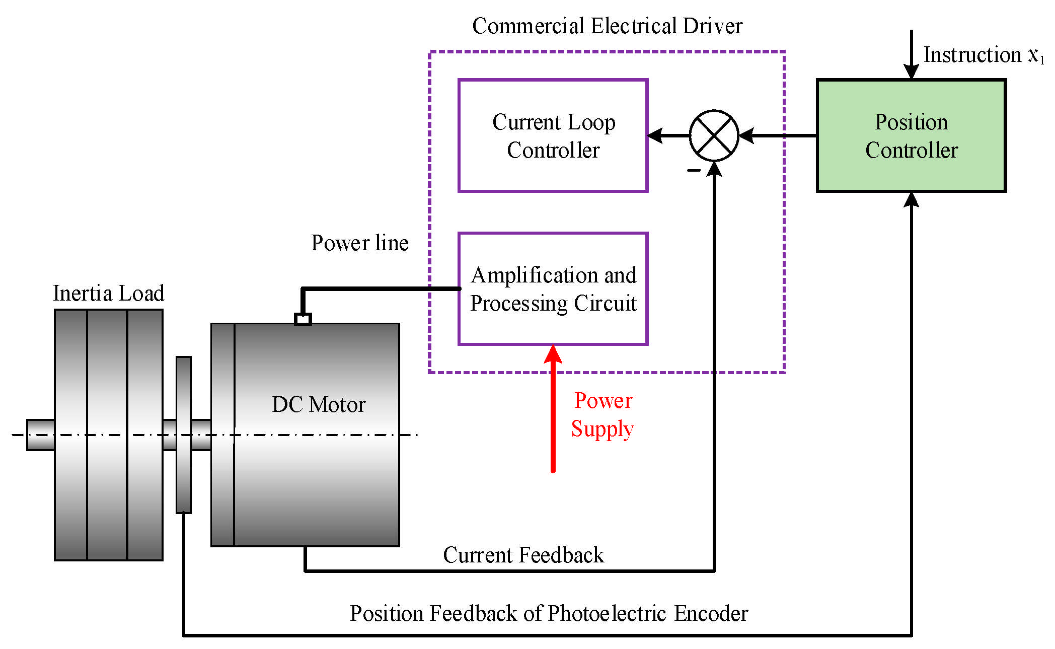
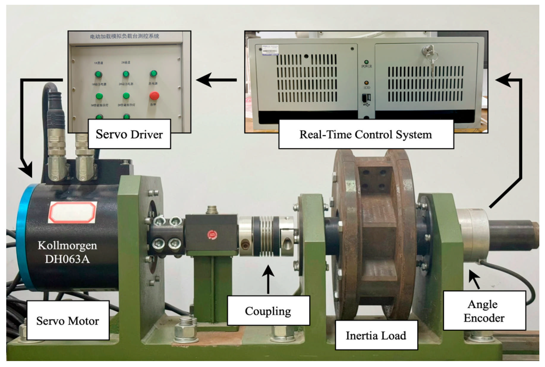
The overall assembly diagram and control system of the experimental platform are illustrated in Figure 3, with the component list and motor specifications detailed in

Table 1. Experimental system components list.

Component List	Specifications
Motor	Kollmorgen D063M-13-1310
Servo drive	Kollmorgen ServoStar 620
Rotary encoder	Heidenhain ERN180 rotary encoder
Torque sensor	CD1140 Series Torque Sensor
Coupling	JB/ZQ4376-86 YL1 Type Flange Rigid Coupling
Inertia	0.31 kg·m2
Motor torque	0.8806 $\mathrm{N}\mathrm{m}/\mathrm{A}\mathrm{r}\mathrm{m}\mathrm{s}$
Maximum speed of the motor	500 $\mathrm{R}\mathrm{P}\mathrm{M}$
Maximum voltage of the motor	240 Vrms

. The platform comprises the following core components: a base unit, a PMSM drive system (including Kollmorgen D063M-13-1310 PMSM, Kollmorgen ServoStar 620 servo drive (Kollmorgen Corporation, Radford, VA, USA), Heidenhain ERN180 rotary encoder with ±13 arcsec accuracy (Heidenhain GmbH, Traunreut, Germany), inertia flywheel and coupling mechanism), power supply module, and measurement-control system. The measurement-control system integrates monitoring software with an industrial computer running real-time operating system RTU, which executes control programs developed in C language. Hardware interfaces include an Advantech PCI-1723 16-bit D/A conversion card for control command output and a Heidenhain IK-220 16-bit acquisition card for encoder signal collection. With a control cycle of 0.5 ms, the system velocity is calculated in real time through backward difference algorithm based on high-precision position signals.

6.1. Overview of Proposed and Comparative Controllers

To compare the effectiveness of the proposed algorithm, the following five controllers were implemented for comparative experiments under the same conditions:

C1: To adjust the proposed BCF-RL controller, the parameters of the BCF main controller were first determined according to Theorem 1 to ensure fast response and stability. Then, the RL auxiliary controller was integrated, and its parameters were adjusted to achieve fast convergence of the neural network. Finally, we fine-tuned the parameters to optimize the overall control performance. After the calculation, the control parameters were determined as follows: $k_1=160,k_2=45,l_{a1}=1,l_{a2}=0.4,l_{a3}={2,l}_{a4}=0.2,l_{c1}=1$, $l_{c2}=0.3,l_{c3}={1,l}_{c4}=0.1.$ The number of hidden layers in the neural network was five. The initial weight value of the neural network was set to 0.1 for each element. Through friction fitting experiments, the parameters of the friction model $T_f$ are obtained as follows: $a_1=2,a_2=0.88,a_3=3.39,c_1=39.3,c_2=834,c_3=1550.$ The controller gains $k_1,k_2$ of C2–C4 are the same as those in C1.

C2: The BCF-SNN controller estimates unknown dynamics using a single-actor neural network (SNN). Unlike the proposed controller, it does not include a critic network for evaluating the actor network. The control law is shown in (65).

$$\begin{array}{cc}\hfill u& =-(-\widehat{F}-{\dot{\widehat{\alpha }}}_1-\beta \phi (x_2)+e_1+k_2{e}_2)/K,\hfill \\ \hfill e_1& =x_1-{\alpha }_0,e_2=x_2-{\alpha }_1,{\alpha }_1=x_2-{\dot{\widehat{e}}}_1-k_1{e}_1,\hfill \\ \hfill \widehat{F}& ={\widehat{W}}_2\phi ,{\dot{\widehat{W}}}_2=-\Gamma E\phi ,E={\dot{\widehat{e}}}_2+e_1+k_2{e}_2\hfill \end{array}$$

(65)

To ensure a fair comparison, the initial weight value of the BCF-SNN controller was set to be the same as that of the BCF-RL controller.

Remark 2. 

The neural networks used in this study feature a shallow architecture, resulting in lower computational complexity than deep neural networks. They are implemented in C language and executed on a real-time control system.

C3: Extended state observer (ESO) is a classic method for estimating states and system disturbances. To further compare the estimation performance of the disturbances, the neural network in C2 was replaced with an ESO for disturbance estimation. The specific design of the ESO can be found in [19]. The ESO bandwidth was set to ${\omega }_0=150$.

C4: The BCF controller, which does not include a neural network compared with the BCF-RL, has the control law shown in (66).

$$\begin{array}{cc}\hfill u& =-(-{\dot{\widehat{\alpha }}}_1-\beta \phi (x_2)+e_1+k_2{e}_2)/K,\hfill \\ \hfill e_1& =x_1-x_d,e_2=x_2-\alpha ,{\alpha }_1=x_2-{\dot{\widehat{e}}}_1-k_1{e}_1\hfill \end{array}$$

(66)

C5: The traditional PID controller follows the control law expressed in (67).

$$u=k_{p}e+k_i{\displaystyle \int e\mathrm{d}t}+k_d\dot{e},e=x_d-x_1$$

(67)

The PID control parameters were set as $k_p=57,k_i=145.355$ and $k_d=5.633$. These parameter values were determined using the typical Type-II system methodology for PID controller tuning and have been validated through simulation experiments.

6.2. Verification of Disturbance Estimation

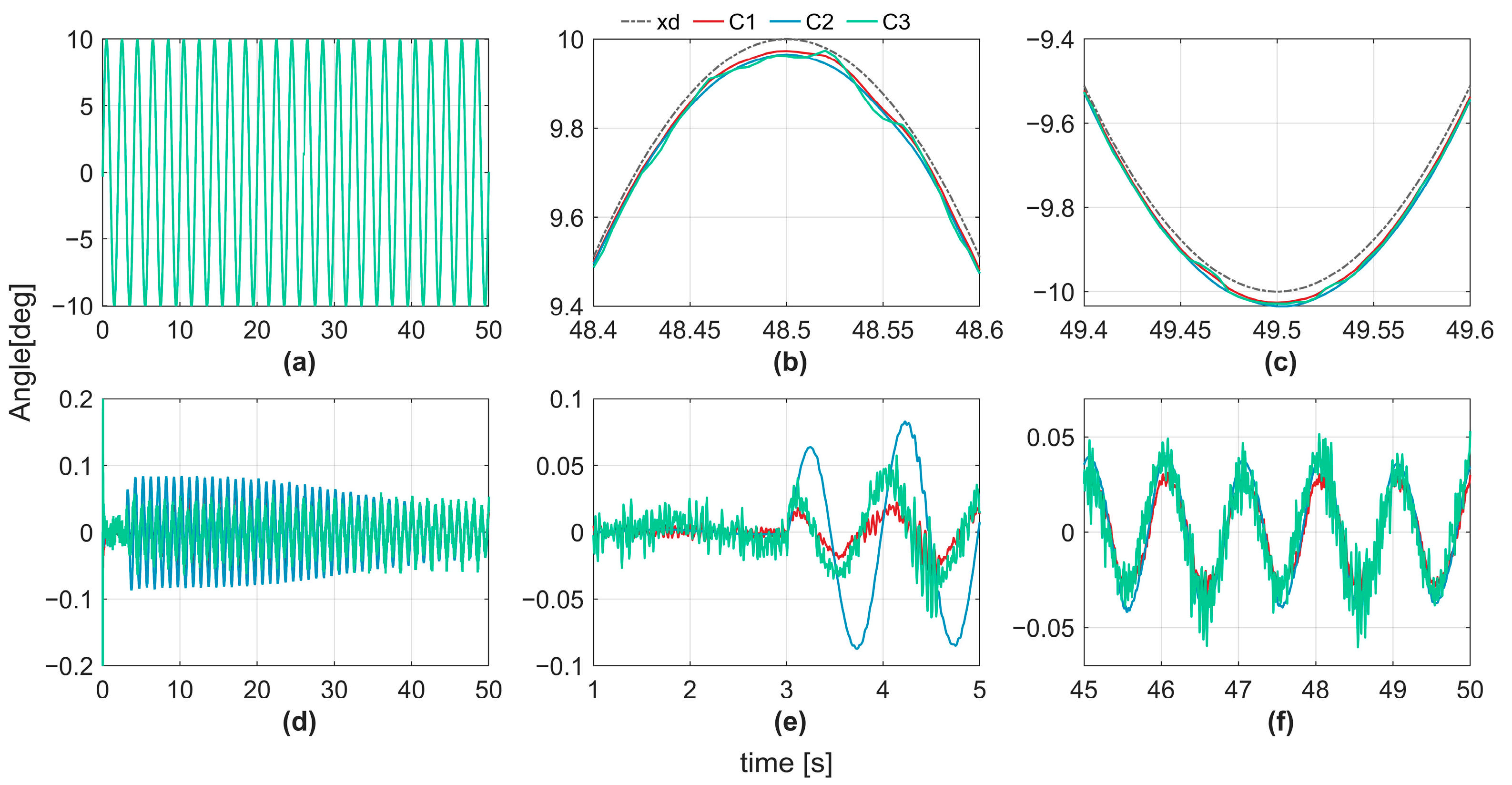
Simulations were conducted using the MATLAB/Simulink (2023b) software. Three controllers (C1, C2, C3) are compared in this study. The comparison between C1 and C2 evaluates the performance of the actor-critic mechanism implemented in C1. C3 employs a classical Extended state observer (ESO) for disturbance estimation. Because of the unmeasurable nature of unknown dynamics in real systems, the evaluation of disturbance estimation is conducted solely through simulations. In the simulation, the desired trajectory is defined as $x_d=10sin\left(\pi t\right)$(deg), with the unknown disturbance set to zero during the first 3 s and introduced at $t\ge 3$ as $f\left(t\right)={0.003x}_1{x}_2$ (Nm).

The tracking trajectories and errors of the three controllers are shown in Figure 4. Figure 4a shows the tracking curves of the four controllers. Figure 4b and Figure 4c show zoomed-in views of the last crest and trough regions in Figure 4a, respectively. Figure 4d presents the tracking error curves of the four controllers. To better observe the tracking performance immediately after the disturbance introduced at the 3 s mark, Figure 4e displays a zoomed-in view of Figure 4d over the 1–5 s interval. It can be observed that before the disturbance occurs, C3 exhibits the largest tracking error, followed by C3, whereas C1 achieves the smallest errors with minimal differences. Figure 4f illustrates the zoomed-in tracking errors during the steady-state phase (45–50 s), showing that C3 has similar maximum tracking errors. Benefiting from the neural network’s more accurate disturbance estimation, the tracking errors of C2 and C1 were significantly reduced. In particular, C1, with its actor-critic mechanism, achieves the smallest tracking error. The maximum steady-state tracking errors for C1, C2, and C3 are 0.038°, 0.043°, and 0.06°, respectively.

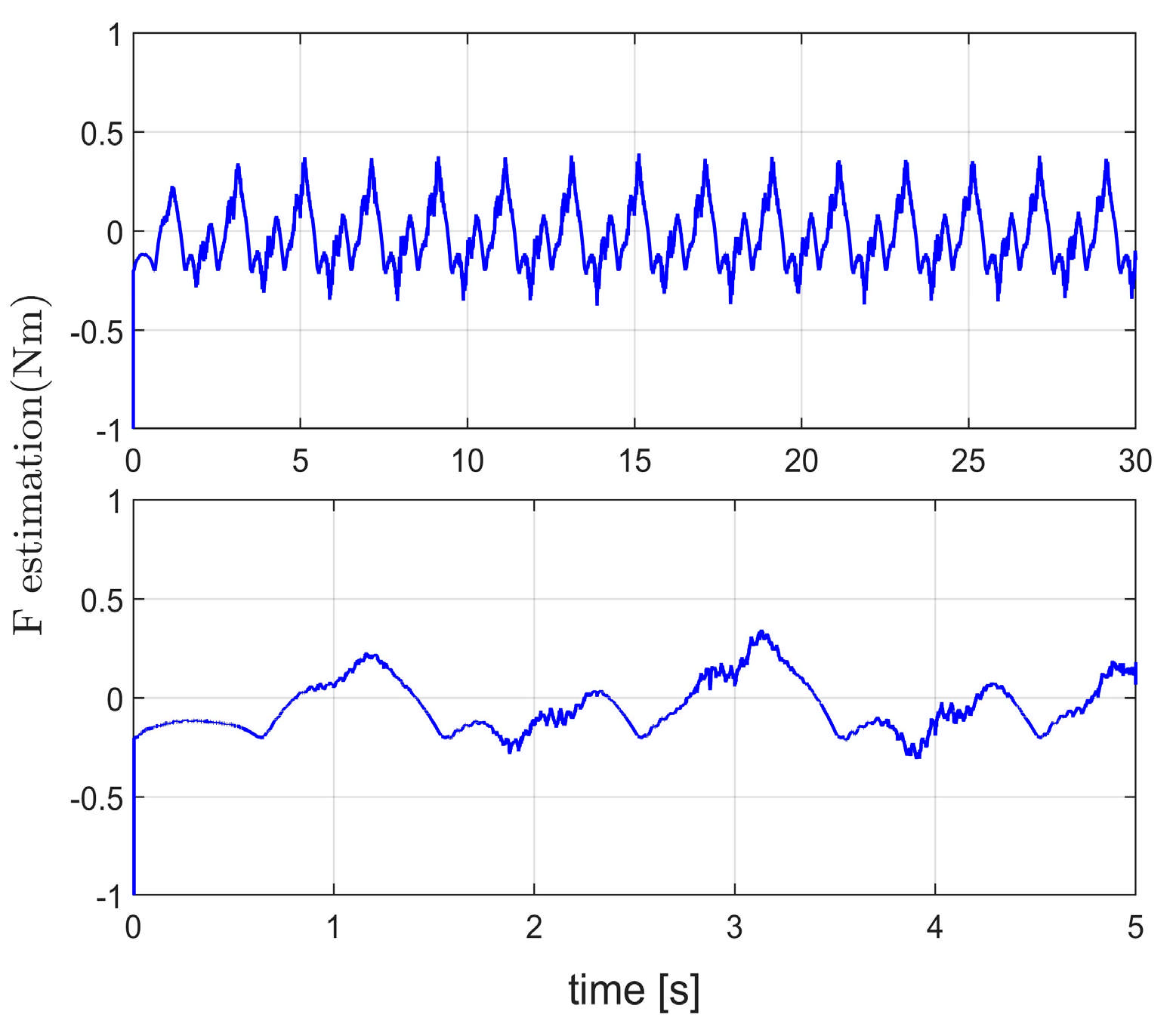
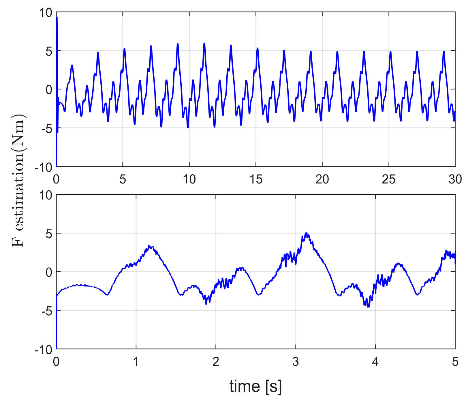
Figure 5 illustrates the estimation trajectories and errors of the unknown disturbances for the three controllers. Figure 5b and Figure 5c show zoomed-in views of the last crest and trough regions in Figure 5a, respectively. Figure 5d shows the tracking error curves of the unknown disturbances, while Figure 5e presents a zoomed-in view of Figure 5d over the 1–5 s interval. It can be observed that in the absence of disturbances, the disturbance estimation errors of the three controllers fluctuate around zero. After the disturbance is introduced at the 3 s mark, C1 achieves the smallest estimation error, followed by C3 and C2. Figure 5f highlights the steady-state phase (45–50 s), where C1 still maintains the smallest estimation error, C2 ranks second, and C3 has the largest error. Although C3 initially converges faster when estimating unknown disturbances, its steady-state accuracy is inferior to that of C1 and C2. Additionally, C3’s estimation curve exhibits persistent oscillations, which are less smooth than those of C2 and C1, potentially imposing extra computational burdens on the system. The superior estimation accuracy of C1 over C2 further validates the effectiveness of the proposed actor-critic mechanism in C1.

Table 2. Performance in simulation.

Indices	C1	C2	C3
M	0.0354	0.0426	0.0602
μ	0.0182	0.0243	0.0217
σ	7.06 × 10−5	1.39 × 10−4	1.57 × 10−4
Mo	1.2270	1.6278	2.1652
μo	0.6017	0.8056	0.7487
σo	0.0793	0.1623	0.1824

presents the results. The primary performance metrics include the maximum absolute tracking error (M), average tracking error (μ), and standard deviation of the tracking error (σ), as defined in [19]. The subscript ‘o’ indicates the analysis term for an unknown dynamic estimation error. Figure 6 shows a bar chart derived from the normalized data presented in Table 2. Both Table 2 and Figure 6 indicate that all indicators of C1 surpassed those of C2 and C3.

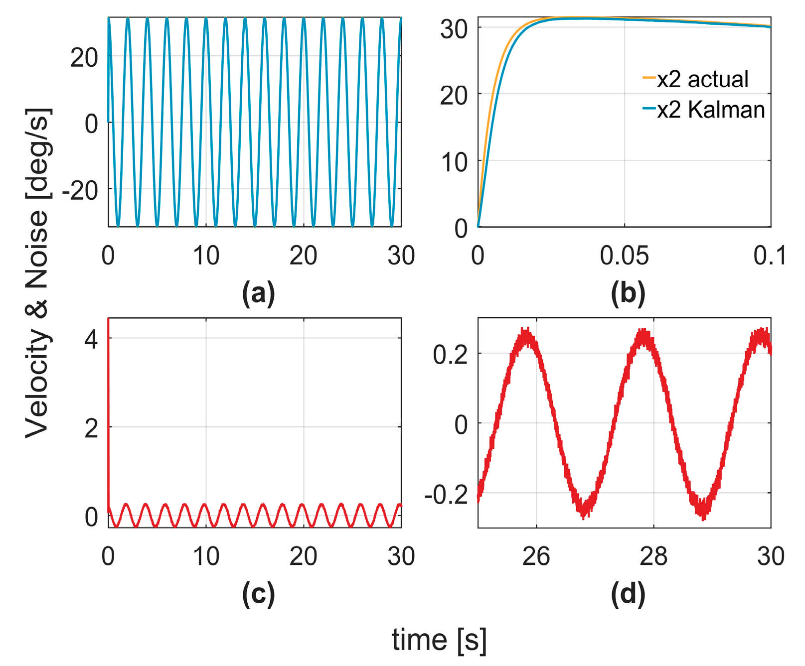
6.3. Verification of Handling System Noise

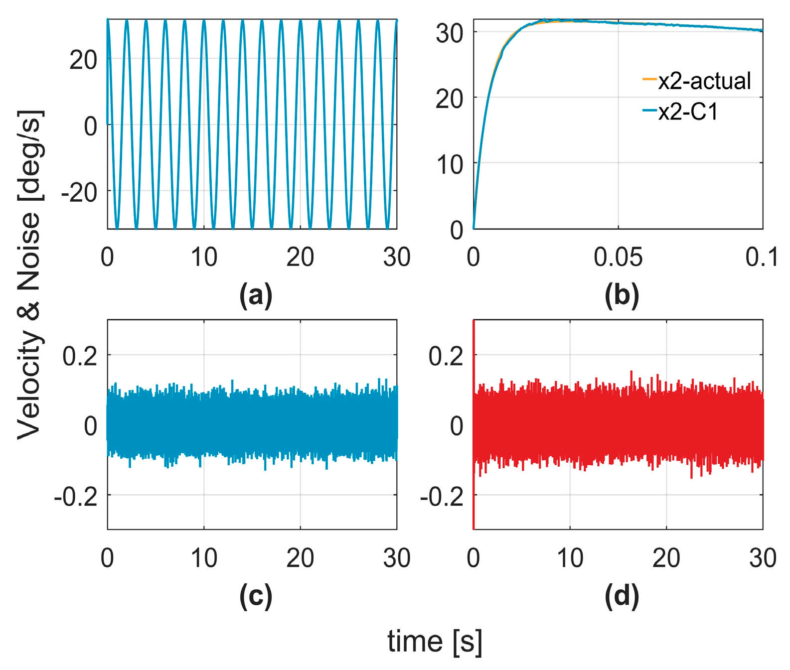
To verify the effectiveness of the controller in handling the system noise, a comparative analysis with a Kalman filter was conducted. Figure 7a,b illustrates the velocity estimations generated by the Kalman filter. Figure 7c,d depicts the estimation errors, representing the differences between the estimated and actual velocities, which correspond to the estimated noise signals. Figure 8a,b shows the velocity estimations produced by the C1 controller, whereas Figure 8d displays the noise signals estimated using Equation (11). Figure 8c shows the artificially introduced noise signals added to the system. By comparing Figure 7d and Figure 8d, it is evident that the proposed method not only achieves more accurate noise signal estimation, but also generates smoother estimation curves, significantly mitigating the impact of noise on the system. This demonstrates that the proposed method outperformed the Kalman filter in terms of noise suppression and system robustness.

6.4. Verification of Tracking Performance

Five controllers were evaluated for tracking performance of the desired trajectory $x_d=10sin\left(\pi t\right)$(deg).

6.4.1. Case 1: No Additive Disturbance

Figure 9 compares tracking errors in Case 1. Controller C5 exhibited the maximum steady-state error (0.074°), followed by C4 (0.062°). With reduced disturbance effects, C3 achieved a lower maximum steady-state error (0.056°) than the former two controllers. Through neural network-based estimation and compensation for unknown dynamics, C2 and C1 demonstrated higher precision. Particularly, C1 with critic neural network integration achieved optimal tracking performance (maximum steady-state error: 0.041°). Figure 10 compares controller energy consumption. Figure 11 verifies real-time implementation of the RL-augmented controller. Figure 12 shows rapid convergence of actor network weights under disturbance-free conditions.

Table 3. Performance of controllers under Case 1.

Indices	M	μ	σ	Eu
C1	0.0409	0.0149	0.0182	0.9384
C2	0.0444	0.0164	0.0201	0.9382
C3	0.0557	0.0203	0.0257	0.9324
C4	0.0618	0.0213	0.0271	0.9268
C5	0.0735	0.0313	0.0332	0.9273

demonstrates the superiority of the proposed C1 controller across all key performance indicators (M is maximum steady-state error; μ is mean error; σ is the standard deviation of error). The root mean square of control input (Eu) reflects energy consumption. Comparative analysis reveals that C4 exhibits greater robustness than C5. However, because C4 lacks disturbance estimation compensation, its control precision is lower than that of C1–C3. Due to critic-actor structure, C1 achieves higher tracking accuracy compared to C2, which relies solely on a single neural network for disturbance estimation. While C2 demonstrates slightly lower energy consumption than C1, C1 outperforms C2 significantly with a 9% lower M value for critical performance metrics.

6.4.2. Case 2: Position–Velocity–Input Disturbance

Considering the diversity and complexity of actual working conditions, position–velocity–input interference is used to test the control effect of the controller, that is, the actual input of the plant is 0.5u − 0.2x₁ + 0.05x₂. Compared with Case 1, there are significant changes in the structural and unstructured uncertainties in this situation.

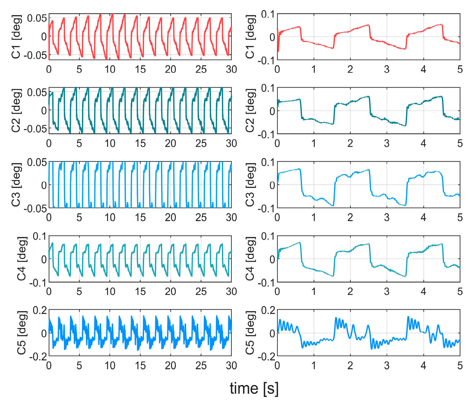
As shown in Figure 13 and

Table 4. Performance of controllers under Case 2.

Indices	M	μ	σ	Eu
C1	0.0532	0.0352	0.0367	0.9896
C2	0.0637	0.0402	0.0435	0.9857
C4	0.0748	0.0425	0.0456	0.9931
C5	0.0841	0.0519	0.0542	0.9786
C6	0.1206	0.0661	0.0658	0.9759

, under complex conditions, C5 exhibits the largest steady-state tracking error of 0.12°, while the improvement of C4 is limited. Compared with C5 and C4, C3 achieves a 37% and 11% reduction in error, respectively. By employing neural network-based disturbance estimation and compensation, C2 further reduces the error to 0.064°. C1 achieves the lowest tracking error of 0.05°. 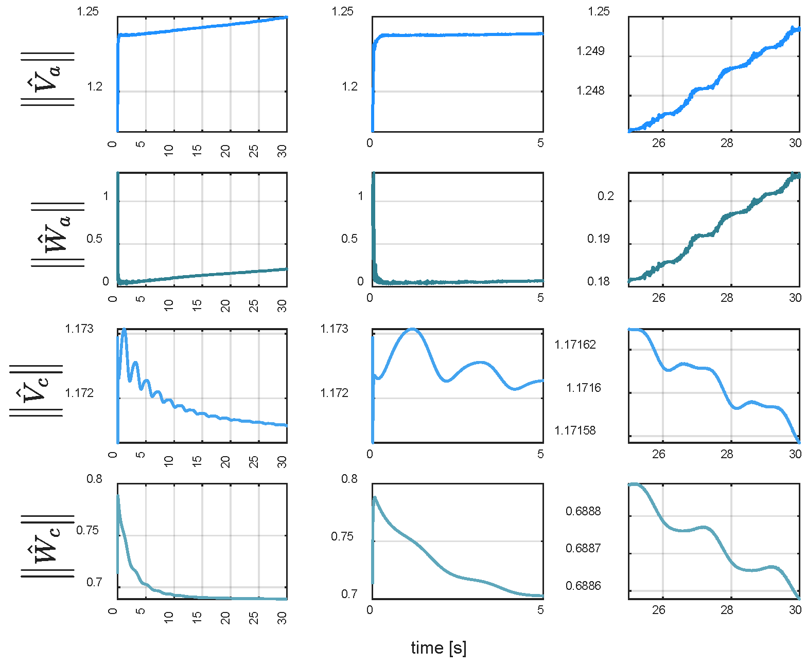The comparison of control inputs in Figure 14 confirms that C1 achieves the best tracking while maintaining low energy consumption. 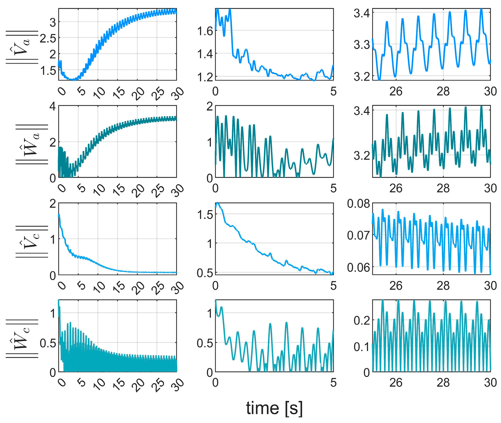The disturbance estimation in Figure 15 and the variation of weight norms in Figure 16 reveal that, despite the increased complexity, the actor-critic network remains convergent, and the reinforcement learning-assisted controller ensures stable operation under adverse conditions.

6.4.3. Confidence Interval and t-Test Analysis

To ensure the reliability of the experimental results, this study conducted repeated experiments on five controllers (C1–C5) under Case 2, collecting 20 trajectory tracking error samples for each controller. At a 95% confidence level (α = 0.05), the confidence interval was calculated based on the t-distribution using the following formula:

$${\overline{e}}_i\pm t_{\alpha /2,n-1}·{\displaystyle \frac{s_i}{\sqrt{n}}}$$

where ${\overline{e}}_i$ represents the mean tracking error of the i-th controller, $s_i$ denotes the standard deviation of the corresponding controller’s tracking error, and the sample size n = 20. Consulting the t-distribution table, with degrees of freedom n − 1 = 19, the critical value $t_{\alpha /2,n-1}$ = 2.093.

The confidence interval analysis presented in

Table 5. Confidence Interval Analysis of Controllers under Case 2.

Indices	${\overline{\mathit{e}}}_{\mathit{i}} \left(\mathbf{d}\mathbf{e}\mathbf{g}\right)$	${\mathit{s}}_{\mathit{i}}$	Confidence Interval (95%)
C1	0.0418	0.0191	[0.0329, 0.0507]
C2	0.0474	0.0211	[0.0375, 0.0573]
C3	0.0578	0.0277	[0.0448, 0.0708]
C4	0.0644	0.0289	[0.0509, 0.0779]
C5	0.0835	0.0350	[0.0671, 0.0999]

indicates that C1 exhibits the lowest mean tracking error (0.0418 deg) and the narrowest confidence interval ([0.0329, 0.0507]), demonstrating the smallest error and highest stability. In comparison, C2 has a slightly higher mean (0.0474 deg) and a marginally wider interval ([0.0375, 0.0573]); the confidence intervals of C3, C4, and C5 progressively increase in both mean and width, with C5 showing the highest mean (0.0835 deg) and the widest interval ([0.0671, 0.0999]), indicating the greatest variability. Overall, C1 outperforms C2, C3, C4, and C5 in terms of both mean error and stability, making it the optimal controller among the five.

To further quantify the performance advantage of the C1 controller, this study employed an independent samples Welch’s t-test (two-sample t-test assuming unequal variances) for inter-group difference analysis. As shown in

Table 6. t-Test Results for Controllers under Case 2.

Compare	${\overline{\mathit{e}}}_1-{\overline{\mathit{e}}}_{\mathit{i}}$	t-Value	Critical t-Value	Reject H0?
C1 vs. C2	−0.0056	−0.881	−1.686	No
C1 vs. C3	−0.016	−2.128	−1.686	Yes
C1 vs. C4	−0.0226	−2.916	−1.686	Yes
C1 vs. C5	−0.0417	−4.675	−1.686	Yes

, using C1 as the baseline, one-tailed tests (α = 0.05) were conducted against C2–C5. The null hypothesis $H_0$ was defined as ${\overline{e}}_1={\overline{e}}_i$, indicating no difference in mean error between C1 and the i-th controller; the alternative hypothesis $H_1$ was ${\overline{e}}_1<{\overline{e}}_i$, suggesting that C1’s mean error is less than that of the iii-th controller. The one-tailed critical t-value, based on degrees of freedom $2n-2=38$, was approximately −1.686 from the t-distribution table. The t-value was calculated using the following formula:

$$t_i={\displaystyle \frac{{\overline{e}}_1-{\overline{e}}_i}{\sqrt{\frac{s_1^2+s_i^2}{n}}}}$$

The statistical results in Table 6 indicate that, at a 95% confidence level, the mean error difference between C1 and C2 did not reach statistical significance (t = −0.881), failing to reject $H_0$. However, C1 demonstrated a significant advantage over C3, C4, and C5, with t-values of −2.128, −2.916, and −4.675, respectively, all below the critical value of −1.686–1.686−1.686. The negative mean differences (−0.016, −0.0226, and −0.0417) further confirm that C1’s tracking error is significantly lower than that of these controllers. Based on the hypothesis testing results, C1 exhibits statistically significant superiority in trajectory tracking performance, establishing it as the optimal controller.

7. Conclusions

Considering the challenges in establishing accurate dynamic models for electromechanical servo systems and the sensitivity of system state information measurements to noise, this study proposes a nonlinear backstepping control algorithm that integrates a command filter with RL. This control algorithm effectively addresses the issues of measurement noise, unmodeled disturbances, and external interference in electromechanical servo systems by leveraging the command filter and RL. The weight update law of the RL neural network is implemented online using a gradient descent algorithm. Stability analysis and proof of the closed-loop system were conducted based on the Lyapunov function method. Comparative experiments were performed to validate the effectiveness of the designed controller, and confidence intervals and t-tests were employed to verify the reliability of the controller. The experimental results demonstrate that the proposed algorithm exhibits strong robustness against system uncertainties and external disturbances, achieving excellent control performance.