A Self-Adaptive Double Q-Backstepping Trajectory Tracking Control Approach Based on Reinforcement Learning for Mobile Robots

Abstract

When a mobile robot inspects tasks with complex requirements indoors, the traditional backstepping method cannot guarantee the accuracy of the trajectory, leading to problems such as the instrument not being inside the image and focus failure when the robot grabs the image with high zoom. In order to solve this problem, this paper proposes an adaptive backstepping method based on double Q-learning for tracking and controlling the trajectory of mobile robots. We design the incremental model-free algorithm of Double-Q learning, which can quickly learn to rectify the trajectory tracking controller gain online. For the controller gain rectification problem in non-uniform state space exploration, we propose an incremental active learning exploration algorithm that incorporates memory playback as well as experience playback mechanisms to achieve online fast learning and controller gain rectification for agents. To verify the feasibility of the algorithm, we perform algorithm verification on different types of trajectories in Gazebo and physical platforms. The results show that the adaptive trajectory tracking control algorithm can be used to rectify the mobile robot trajectory tracking controller’s gain. Compared with the Backstepping-Fractional-Older PID controller and Fuzzy-Backstepping controller, Double Q-backstepping has better robustness, generalization, real-time, and stronger anti-disturbance capability.

1. Introduction

Autonomous navigation and motion controls are essential indicators and core technologies for the autonomy of mobile robots. Mobile robots with autonomous navigation and motion capabilities are widely used in industries such as agriculture, machining, rescue, scientific research, services, and almost all mobile application fields, presenting broad needs and extensive application prospects. In the global revolution of Industry 4.0, increasingly mobile robots assume a critical role in human life. They will also occupy an essential part of industrial production and manufacturing systems. Mobile robots must have the ability to navigate autonomously, make decisions, have good perception, and can accurately complete the tasks required. Furthermore, the working environment of these mobile robots entails various uncertain factors that pose significant challenges to their autonomous navigation and decision-making capabilities.

Wounded rescue missions and critical facility inspections represent typical applications of mobile robots. In such scenarios, to ensure the personal safety of the wounded and the safety of essential facilities, the robot must move quickly, stably, and accurately along the planned trajectory [1]. To fulfill all mission requirements with minimal tracking error, mobile robot trajectory tracking control algorithms that have superior adaptability, real-time capability, and robustness are often necessary to tackle the different expected trajectories. In this domain, the challenges associated with most trajectory-tracking control algorithms remain a subject of intense research [2,3]. Therefore, under the requirements of such tasks, it is imperative to have trajectory tracking control algorithms that can adapt quickly and have real-time capability to cope with dynamic and unpredictable changing environments.

The backstepping controller [4] demonstrates a global stabilization effect in nonlinear and non-holonomic constrained systems, making it a popular choice for a variety of mobile robot platforms [5,6,7,8]. It is widely used to control the trajectory tracking of mobile robots. The adoption of a Backstepping controller in mobile robot systems often involves expert tuning to find the optimal control gain. However, modern control theory provides methods and suggestions for tuning the parameter gain of the Backstepping controller. Wang [9] proposed a new Backstepping controller gain adjustment method that employs compensation terms in the control law to resolve the over-parameterization problem in parameter estimation. Similarly, Wang [10] designed a nonlinear Backstepping controller gain adjustment method based on linearity, separating the linear part from the nonlinear system to form a linear auxiliary system to determine the additional linear system. The state feedback gain is converted into the Backstepping gain through state feedback to determine the gain of the Backstepping controller for the nonlinear system. However, the high-complexity dynamics, high coupling, and nonlinearity of mobile robots lead to difficulties in parameter gain tuning for the Backstepping controller, which often results in poor real-time performance, low control accuracy, and poor robust performance. This usually necessitates expert-level a priori knowledge to make on-line adjustments to the controller parameter gain as per the task requirements and changes in the mobile robot’s operating environment.

The traditional backstepping controller cannot adjust the parameter gain in real time during the trajectory tracking control process of the mobile robot, making it challenging to achieve precise and optimal control of the robot. To address this issue, some researchers have proposed a trajectory-tracking controller with self-adaptive control. Hu [11] proposed a robot tracking controller based on self-adaptive backtracking to solve the tracking control problems of inaccurate Robot Kinematics/Dynamics modeling and external environment disturbance. By designing an appropriate Lyapunov function, the stability of the robot tracking controller is guaranteed. Van [12] proposed and designed a self-adaptive Backstepping robot tracking control algorithm that employs nonsingular fast terminal sliding mode control (NFTSMC) to handle uncertainties, external disturbances, and fault compensation in the robot control system. The controller maintains the merits of NFTSMC with high robustness, fast transient response, and finite-time convergence. However, the primary limitation of this controller is its reliance on prior knowledge of disturbances and uncertainty bounds during the design process. Sun [13] designed a self-adaptive tracking controller that compensates for errors and automatically tunes parameters based on the nonlinear system of mobile robots to solve the trajectory tracking problem of mobile robots with parameter uncertainty. Based on the dynamic model of the mobile robot, a self-adaptive controller based on state feedback is designed by selecting the appropriate Lyapunov function through the pursuit recursive method so that the mobile robot can gradually track the desired trajectory. However, traditional self-adaptive backstepping control algorithms usually cannot achieve optimal robot control under varying robot environments and task requirements, such as underlying drive control of mobile robots, path tracking, and trajectory tracking, requiring expert knowledge and multiple adjustments to obtain optimal controller parameters.

Reinforcement Learning (RL) methods [13], a significant branch of artificial intelligence, have developed rapidly in the field of control. The RL algorithm is an iterative learning process that involves continuous interaction between the robot system and its environment. RL is a hybrid control strategy that employs a reward value function to evaluate action quality during interaction between the robots and their environment. Compared with traditional control algorithms, RL has significant potential advantages; it continually learns the optimal control strategy through the reward value function until the optimal solution surfaces. RL can better solve control problems that are difficult to solve in traditional algorithms owing to its unparalleled robustness, real-time performance, and generalization [14]. Advanced RL methods can address high-dimensional disasters and problems with optimal control policies that are difficult to converge, and achieve exemplary performance in complex environments. Q-learning in RL and its derivatives [15] are among the most widely used and successful RL algorithms, which have found applications in various domains such as mobile robot path planning [16,17], underlying control [18], game development [19,20], natural language processing [21,22], autonomous driving [23,24], and others.

To summarize, many researchers have made significant contributions to the adaptive control of mobile robots in the field of reinforcement learning. Their work involves adapting traditional control algorithms by optimizing their parameters. For instance, Ignacio [25] proposed an incremental Q-learning strategy of adaptive PID control for parameter tuning when the system and operating conditions are unknown and variable. The feasibility of the algorithm is verified by simulation and physical experiments. Ignacio [26] then added a multi-function value update experience replay mechanism to adjust the controller parameters according to the double-q incremental model-free algorithm. After conducting simulation and physical comparison experiments, it has been demonstrated that the proposed algorithm for adjusting the adaptive parameters of the controller has good real-time performance and robustness. However, these experiments only involved ground robots, and thus further research is necessary to determine the algorithm’s feasibility in other scenarios. Cheng [27] exploited the adaptive controller with fast estimation and active compensation capabilities for continuous state and action spaces, improving the success rate of RL control algorithms in different training environments or external disturbances. The controller has strong robustness and can effectively reduce the training time of the controller. Still, it is difficult to obtain an effective solution for continuous action space or high-dimensional action space problems, and it is easy to fall into the trap of local optimality. Subudhi [28] proposed an Actor/Critic-LQR adaptive control method based on reinforcement learning for the adaptive control of multi-link flexible manipulators under different load conditions. The algorithm does not depend on the dynamic model of the system, and the method has less computational complexity than other adaptive control algorithms. However, the disturbance between the robot and the external environment is not considered. Khan S G [29] developed an adaptive control strategy online using a combination of dynamic programming and reinforcement learning for a humanoid robot arm’s two joints (shoulder flexion and elbow flexion). The effect of simulation and physical experiments has been significantly improved. However, compared with the traditional methods, the computation is huge, the control response time is longer, and the requirements for robot hardware are very high.

In the field of RL, the double Q-learning algorithm [30] is widely used in the industry due to its good learning characteristics, which can effectively reduce the typical overestimation in the Q-learning algorithm. Ou [31] proposed a new reinforcement learning-based framework to realize the quadrotor autonomous obstacle avoidance method. A double-depth loop is used to solve the error problem of the observation capability of the airborne monocular camera. Behzad [32] proposed a double Q-learning algorithm to solve the problem of aircraft trajectory optimization. Under the premise of meeting the communication connectivity constraints required for the safe operation of the aircraft, the aircraft can be operated in the shortest time. Through two assumptions: the short-term absence of GPS signal and the problem of the GPS signal missing for a certain period, the feasibility of the algorithm is verified by experiments. Faezeh [33] uses double Q-learning and a* with an offline policy reinforcement learning algorithm to build a new controller. Compared with the traditional A* and Q-learning algorithms, the algorithm is more reliable and has a stronger ability to avoid collisions with obstacles. Khan [34] proposed an algorithm based on deep double Q-learning to solve the motion planning problem of robots in complex environments. By using multiple gaits, the robot is trained to minimize the distance between its current position and the training target point. Extensive tests conducted across various terrains have demonstrated the algorithm’s efficacy in all unknown complex environments with 100% performance efficiency.

Robots controlled by RL and backstepping methods must have high control accuracy for typical complex application situations such as casualty rescue and power facility inspection. In summary, the contributions of this paper are highlighted as follows:

• Aiming at the trajectory tracking control problem of mobile robots, the idea of artificial intelligence is introduced into the backstepping trajectory tracking controller. A control scheme combining backstepping with reinforcement learning is proposed;
• Compared with the traditional algorithm, it is not required for the proposed method to be trained with a large number of samples offline. It achieves high-precision tracking control by fast online learning for controller gain optimization without the expert-level gain adjustment capability.
• The new algorithm combines the double Q-learning incremental discretization strategy with a subregional active learning strategy. In order to improve the learning efficiency, an experience replay mechanism and a time–memory function are introduced for online gain adjustment, so that online learning can be completed faster, and optimal control can be realized.

The rest of the paper is organized as follows: In Section 2, the problem statement is presented. In Section 3, we point out the details of the online gain tuning of the high-accuracy trajectory tracking controller. Section 4 presents the simulation and physical experimental results of this control algorithm. Finally, conclusions are drawn in Section 5.

2. Problem Statement and Analysis

The traditional backstepping trajectory tracking controller is difficult to use to track the desired trajectory with high precision, speed, and stability in an unknown and variable environment. In the past, the parameter gains of the backstepping trajectory tracking controller usually needed to be adjusted repeatedly through numerous experiments with the help of expert-level prior knowledge to achieve optimal control. Therefore, to avoid the tedious process of tuning the controller parameter gains for different tasks. This paper will study a self-adaptive trajectory tracking control method based on double Q-learning to solve the problem of automatic tuning of the parameter gains of the trajectory tracking controller for different task requirements. This section will detail the backstepping trajectory tracking control theory, reinforcement learning theory, and double Q-learning control algorithm. These basic concepts are the basis for our proposed self-adaptive trajectory tracking control for mobile robots.

2.1. Backstepping Trajectory Tracking System for Mobile Robots

2.1.1. Mobile Robot Kinematics Model

Differential mobile robots are underactuated systems with typical non-holonomic constraints. Its typical geometry is shown in Figure 1.

In Figure 1, it is assumed that the center of mass of the mobile robot is located at point $C$. The mobile robot platform has three degrees of freedom in a smooth horizontal plane, defined in the body coordinate system and represented by a vector ${\displaystyle \sum X_{R}C{Y}_R}$. The $X_R$ is the forward direction of the mobile robot, and the $Y_R$ is the lateral movement direction of the mobile robot. The global coordinate system based on the current environment of the mobile robot is ${\displaystyle \sum XOY}$. The heading $\theta$ is the angle between the global coordinate system $X$ and the robot body coordinate system $X_R$. The linear and angular velocities of the robot are ${\nu }_C$ and ${\omega }_C$, which can simplify the motion control of the mobile robot. Therefore, the kinematic equation of the mobile robot can be obtained through analysis [35].

$$\left(\begin{array}{c}\stackrel{•}{x}\\ \stackrel{•}{y}\\ \stackrel{•}{\theta }\end{array}\right)=\left(\begin{array}{cc}\cos \theta & 0\\ \sin \theta & 0\\ 0& 1\end{array}\right)\left(\begin{array}{c}{\nu }_c\\ {\omega }_c\end{array}\right).$$

(1)

In Equation (1), $\stackrel{•}{x},\stackrel{•}{y},\stackrel{•}{\theta }$ represents the $X$ direction linear velocity, the $Y$ direction linear velocity, and $\theta$ angular velocity of the mobile robot.

2.1.2. Calculation of Pose Error of the Mobile Robot

In the mobile robot trajectory tracking control system, two sets of vectors represent the robot’s current and desired poses. The current pose is $P_c={[X_c,Y_c,{\theta }_c]}^T$ and the desired pose is $P_r={[X_r,Y_r,{\theta }_r]}^T$. The desired pose is the target point of the robot, the current pose is the robot’s current position. We express the error configuration vector as $P_e={[X_e,Y_e,{\theta }_e]}^T$. The robot trajectory tracking error model is a vector transformation completed in the global coordinate system ${\displaystyle \sum XOY}$ [36,37].

$$\left[\begin{array}{c}{X}_e\\ Y_e\\ {\theta }_e\end{array}\right]=\left[\begin{array}{ccc}\cos \theta & \sin \theta & 0\\ -\sin \theta & \cos \theta & 0\\ 0& 0& 1\end{array}\right]\left[\begin{array}{c}{X}_r-X_c\\ Y_r-Y_c\\ {\theta }_r-{\theta }_c\end{array}\right]=Te(P_r-P_c).$$

(2)

In Equation (2), $X_e$, $Y_e$,and ${\theta }_e$ represent the $X$ direction error, the $Y$ direction error, and the heading error of the mobile robot. The matrix $\left[\begin{array}{ccc}\cos \theta & \sin \theta & 0\\ -\sin \theta & \cos \theta & 0\\ 0& 0& 1\end{array}\right]$ is the coefficient $Te$ for transforming the global coordinate system into the local coordinate system of the mobile robot.

2.1.3. Mobile Robot Trajectory Tracking Control Scheme

Based on the motion mechanism of the differential mobile robot, an overall control scheme of trajectory tracking based on the Backstepping method is proposed, as shown in Figure 2.

In the trajectory tracking control system, the global input of the system is the robot’s desired trajectory $P_r$, desired velocity and angular velocity $q_{\mathrm{r}}={({\nu }_r,{\omega }_r)}^T$. The global output of the system is the current robot pose $P_c$, and the ultimate goal is to use the “Odometry” sensor to converge the pose error to 0. Then, use the pose error $P_e$ at the current moment, the desired velocity and the angular velocity $q_{\mathrm{r}}={({\nu }_r,{\omega }_r)}^T$ to calculate the velocity and angular velocity $q={(\nu ,\omega )}^T$ input by the robot at the current moment. As shown in Equation (3):

$$q=\left[\begin{array}{c}\nu \\ \omega \end{array}\right]=\left[\begin{array}{c}\nu (P_e,q_r)\\ \omega (P_e,q_r)\end{array}\right].$$

(3)

2.1.4. Mobile Robot Trajectory Tracking Controller

For mobile robot trajectory tracking control systems, backstepping design is a systematic controller synthesis method for uncertain systems. This design method combines the selection of Lyapunov function with controller design using a regression method. The approach has gained significant attention from researchers worldwide because it addresses the uncertainties present in the system. Additionally, the method decomposes a complex nonlinear system into subsystems that are within the system’s capacity, enabling the control of a relatively complex nonlinear system. Due to the non-linear nature of slip and the varying dynamic performance of the wheeled mobile robot with changes in ground friction, a Backstepping algorithm was implemented to realize the trajectory tracking control law of the robot.

According to the mobile robot kinematics model and Backstepping modeling method, it is easy to obtain the tracking control law of the wheeled mobile robot [38,39,40] as follows:

$$\left[\begin{array}{l}v\hfill \\ \omega \hfill \end{array}\right]=\left[\begin{array}{c}{v}_C\cos {\theta }_e+k_1{X}_e\\ {\omega }_c+k_2{v}_c{Y}_e+k_3\sin {\theta }_e\end{array}\right].$$

(4)

In Equation (4), $k_1,k_2,k_3$ are all coefficients greater than zero.

In the field of high-precision trajectory tracking control of mobile robots, the dynamic performance of the robot varies with the environment and the task performed. Therefore, to optimize the controller’s performance, it is essential to establish the robot’s pose error model. Moreover, due to the multi-tasking requirements of tracking trajectories, self-adaptive backstepping trajectory tracking control should also be considered. Self-adaptive backstepping trajectory tracking control can choose the optimal control parameter gain in real time based on the mobile robot’s dynamic performance, task requirements, and interactive environment. This feature is an advantage of reinforcement learning in the field of robot control. Compared to the traditional trajectory tracking control algorithm, a self-adaptive trajectory tracking controller for mobile robots based on reinforcement learning performs better online tuning of the controller gain in real-time as per different task requirements and changes in the environment. In the following section, we discuss in detail the RL formulation applied to adjust the parameter gains of the controller.

2.2. Reinforcement Learning Self-Adaptive Control

2.2.1. Reinforcement Learning Description

In reinforcement learning, we refer to the system modeling of control objects as Markov Decision Processes $(MDP)$ [41]. Specifically, it is a tuple defined by four elements: $\{\mathbb{X},\mathbb{K},P,r\}$; $\mathbb{X}$ is the state space, $\mathbb{K}$ is the action space, $P$ is the state transition probability, and $r$ is the reward value function. In the high-precision trajectory tracking agent control system, the selection of the vector $k\in \mathbb{K}$ at each moment is related to the controller gain. In a Markov chain, any state form can be transferred from one state to another. RL solves the control problem by using the ask-based interactive iteration method to achieve the task goal. In the iterative learning process, the current state is observed $x_{\mathrm{t}}\in \mathbb{X}$, and an action $k_{\mathrm{t}}=(k_1,k_2,k_3)$ is selected. According to the state transition probability $P(x_{t+1}|x_t,k_t)$, the agent transitions from the current state $x_{\mathrm{t}}$ to $x_{t+1}$. Moreover, the agent receives the reward function $r_{t+1}(x_t,k_t)$ while the state transitions. The cumulative reward $G_t$ obtained by the agent at the end of the control process is given in Equation (5):

$$G_t=R_{t+1}+\gamma R_{t+2}+\dots =\sum _{k=0}^{\infty }{\gamma }^k{R}_{t+k+1},$$

(5)

where $\gamma$ is the discount factor, which represents the value of future rewards at the moment. The closer $\gamma$ is to 0, the more attention is paid to current interests; The closer you get to 1, the more you value future returns. The purpose of the agent in RL is to find an optimal strategy and select the optimal controller parameter gain $k_{\mathrm{t}}$ according to the system state $x_{\mathrm{t}}$ according to different task requirements to maximize the cumulative reward when the agent reaches the target state. As shown in Equation (6):

$$J^{\ast }=\max J_{\pi }=\max E_{\pi }\left\{R_{t+1}\mid x_t=x\right\}.$$

(6)

Then, we define the optimal state-action value function is given in Equation (5):

$$Q^{\ast }\left(x_t,k_t\right)=E\left\{r_{t+1}+\gamma \underset{k}{\max }{Q}^{\ast }\left(x_{t+1},k_{t+1}\right)\mid x_t,k_t\right\}.$$

(7)

In Equation (7), when the agent transitions from state $x_t$ to $x_{t+1}$, $r_{t+1}$ is the reward value obtained by the system, and $\gamma$ is the same discount factor as appears in Equation (5). Then, when the agent interacts with the environment through the RL Equation to learn the action of the optimal state–action function, the optimal policy can be directly obtained in Equation (8):

$${\pi }^{\ast }=\arg \underset{k}{\max }{Q}^{\ast }\left(x_t,k\right).$$

(8)

2.2.2. Double Q-Learning of Adaptive Backstepping

In Section 1, the origin development and successful application cases of the Double Q-learning algorithm have been described in detail. In the traditional Q-learning learning algorithm, the reward function $r_{t+1}$ has a random Q value, which leads to an overestimation problem. Therefore, the Double Q-learning algorithm decouples the action selection from the Q-value estimation and saves two independent Q-values to update each other through the dual estimator of the Q function, thereby reducing the deviation of the value estimation. That is, if the agent uses Equation (8) to select the optimal action $k_{\mathrm{t}}$ in state $x_{\mathrm{t}}$ and then brings it into the Q-learning algorithm to update the value to $Q_A\left(x_t,k_t\right)$. As shown in Equation (9):

$$Q_A\left(x_t,k_t\right)\leftarrow Q_A\left(x_t,k_t\right)+\alpha \left[r_{t+1}+\gamma \underset{k}{\max }{Q}_B\left(x_{t+1},k_{t+1}\right)-Q_A\left(x_t,k_t\right)\right].$$

(9)

Alternatively, when the agent is in the state $x_{\mathrm{t}}$, use Equation (8) to select the optimal action $k_{\mathrm{t}}$ and to bring it into the Q-learning algorithm to update the value $Q_B\left(x_t,k_t\right)$. As shown in Equation (10):

$$Q_B\left(x_t,k_t\right)\leftarrow Q_B\left(x_t,k_t\right)+\alpha \left[r_{t+1}+\gamma \underset{k}{\max }{Q}_A\left(x_{t+1},k_{t+1}\right)-Q_B\left(x_t,k_t\right)\right],$$

(10)

where $\alpha \in (0,1]$ is the learning rate and $\gamma \in (0,1]$ is the discount factor.

According to the previous analysis and Formulas (9) and (10), it can be seen that the updates of the $Q_A\left(x_t,k_t\right)$ and $Q_B\left(x_t,k_t\right)$ are in the opposite order. The value function A of the optimal action is used to update B, and vice versa. Therefore, each agent update considers the maximum expected payoff of the optimal action policy in a single estimator without necessarily being the best. Two Q-function estimators are used to correct the bias against each other, thereby eliminating the bias problem in overestimation. The Double Q-learning algorithm has the same update characteristics as the Q-learning algorithm. There is no need to open up a considerable amount of computing space not only to ensure the real-time performance of the algorithm but also to maintain the characteristics of the original Q-learning algorithm. In terms of computational complexity and control accuracy, using the Double Q-learning algorithm can effectively reduce the occurrence of overestimation and improve the control accuracy of the system compared to using the Q-leaning algorithm.

2.2.3. Incremental Discretization of State Space and Action Space

In standard Q-learning or double Q-learning algorithms, it is essential to establish a table for state–action discretization. However, if the discretization interval is too large, the agent’s control accuracy may not be high enough, while a small interval may lead to ideal control accuracy but poor time-varying performance. Therefore, many researchers have explored function estimators as an alternative. Wright [42] uses samples collected in the problem domain to reduce the adverse effects of errors. However, the experimental results of using this algorithm are closely related to the sample quality, and the calculation of numerous samples also significantly increases the computational burden of the system [43], which is not suitable for the real-time performance requirements of mobile robot systems. To this end, we propose a novel incremental discretization learning method for state space and action space. This method is based on the incremental discretization idea proposed by Carlucho et al. In this section, we only briefly introduce the concepts related to incremental discretization.

Assuming that the mobile robot is in a two-dimensional Cartesian coordinate system and $\mathbb{X}$ represents the error data set as the state space set, $\eta \left(x_t,x_t{}_{+1}\right)$ represents a value function, and $\rho$ represents a threshold scalar data to determine whether the error at each moment is in the current error set. The agent trajectory tracking control system will change the state of the system from $x_t$ to $x_{t+1}$ over time. In the agent control system, we expect the error between the actual trajectory and the expected trajectory of the robot to approach zero. However, low control accuracy will lead to significant errors. The higher the number of state increment sets $\mathbb{X}$, the greater the computational load on the agent control system. Therefore, to solve the problem of too much data in the incremental discretization set of the state space of the trajectory tracking control system of the agent, it is necessary to divide the incremental state set into three-state spaces, namely (0–0.2], (0.2–0.5], (0.5–∞). After the positional relationship between the current agent state space $x_{t+1}$ and the state increment set $\mathbb{X}$ in the Cartesian coordinate system is determined, the function $\eta \left(x_t,x_t{}_{+1}\right)$ must be used to determine whether the current state set is in the state increment set $\mathbb{X}$. If $\eta \left(x_t,x_t{}_{+1}\right)>\rho$ $\forall x_t\in \mathbb{X}$, then the position information of $x_t$ needs to be added to the state increment set $\mathbb{X}$, namely $\mathbb{X}=\{\mathbb{X}\cup x_{t+1}\}$. If the current system $x_{t+1}$ is in the state increment set $\mathbb{X}$, the discretization process of the state space can be performed. According to the three regions divided by the state increment set $\mathbb{X}$, each maximum discrete level of the state space is 4, 2, and 1, and finally denoted as ${\Lambda }_1=({\rho }_0,{\rho }_1,{\rho }_2,{\rho }_3)$, ${\Lambda }_2=({\rho }_0,{\rho }_1)$, ${\Lambda }_3=({\rho }_0)$.

With the interaction between the agent and the environment and the continuous deepening of learning, the agent must adjust the parameter gains of the backstepping trajectory tracking controller in real-time according to the task requirements and performance indicators. In the Double Q-learning algorithm, at any time $t$, the agent must select a current optimal action $k_{\mathrm{t}}$ from the given action space $\mathbb{K}$ in the Q table through the optimal policy ${\pi }^{\ast }$. In the same way as the discretization of the state space, we discretize the action space to solve the problems of low control accuracy, excessive calculation, and inaccurate establishment of the Q table. As the agent interacts with the environment and continues to learn, the control effect improves after the action space is discretized, allowing for the selection of an optimal action to be applied to the trajectory-tracking controller. This idea is presented in a simple diagram, as shown in Figure 3.

First, assume that the agent is in the state $x_t$, select the optimal action $k_{\mathrm{t}}$ at the current moment in the action space $\mathbb{K}$ according to the optimal strategy and execute (in Figure 3, the blue shaded part represents the optimal action). Then, we assume that the agent interacts with the environment and learns under ideal conditions from the current state $x_t$ to $x_{t+1}$. In the current state, the agent selects the optimal action $k_{\mathrm{t}}$ at the current moment in the action space $\mathbb{K}$ again according to the optimal strategy and executes it. By analogy, according to the discretization criterion of the state space $\mathbb{X}$, if the system state $x_t=x_{t+1}=x_{t+2}=\dots$ remains unchanged, after $n$ cycles, the agent selects the same action $k_{\mathrm{t}}=k_{\mathrm{t}+1}=k_{\mathrm{t}+2}=\dots$ according to the optimal strategy in the action space and executes it. We take the current action. The action space $\mathbb{K}$ is discretized to obtain a more refined action space ${\mathbb{K}}^{\prime }$, which is called the action space incremental discretization process. As shown in Figure 3, after $L$ times of discretization, the final graceful action discretization space is obtained. It is worth noting that during the discretization process of the active learning of the agent, the state of the system at each moment remains unchanged according to the discretization criterion of the state and action of the agent. Finally, the discretization process of the action space is the same as that of the state space and can be carried out to the maximum level $L$; that is, each action space is discretized as $\Delta ={\delta }_1,{\delta }_2,\dots ,{\delta }_L$.

3. Self-Adaptive Trajectory Tracking Control Algorithm Based on Reinforcement Learning

When the mobile robot performs high-precision tracking along the desired trajectory, each time $t$ of the tracking control is related to the error between the desired trajectory and the mobile robot, which not only satisfies the Markov chain but also changes in real-time. In this paper, we consider the specific task of tracking the desired trajectory as a Markov decision process: at the moment $t$, the state $x_t$ of the agent selects and executes an action $k_{\mathrm{t}}$ according to the optimal policy ${\pi }^{\ast }$, which is used as the parameter gain of the current trajectory tracking controller to realize the adaptive adjustment of the speed and angular velocity of the mobile robot. Then, the state $x_{\mathrm{t}+1}$ of the agent at time $t+1$, the reward $r_{t+1}(x_t,k_t)$ at the current time $t$, the action $k_{\mathrm{t}}$, and the state $x_{\mathrm{t}}$ are recombined into a new tuple $(x_{\mathrm{t}},k_{\mathrm{t}},x_{\mathrm{t}+1},r_{t+1})$. Using the idea of backstepping trajectory tracking control, combined with the Double Q-learning algorithm, state space subregion, action space incremental discretization active learning mechanism, the parameter gain of the backstepping controller is self-adjusted through the online learning strategy to ensure the mobile robot can complete the trajectory tracking task with multiple types and high accuracy. 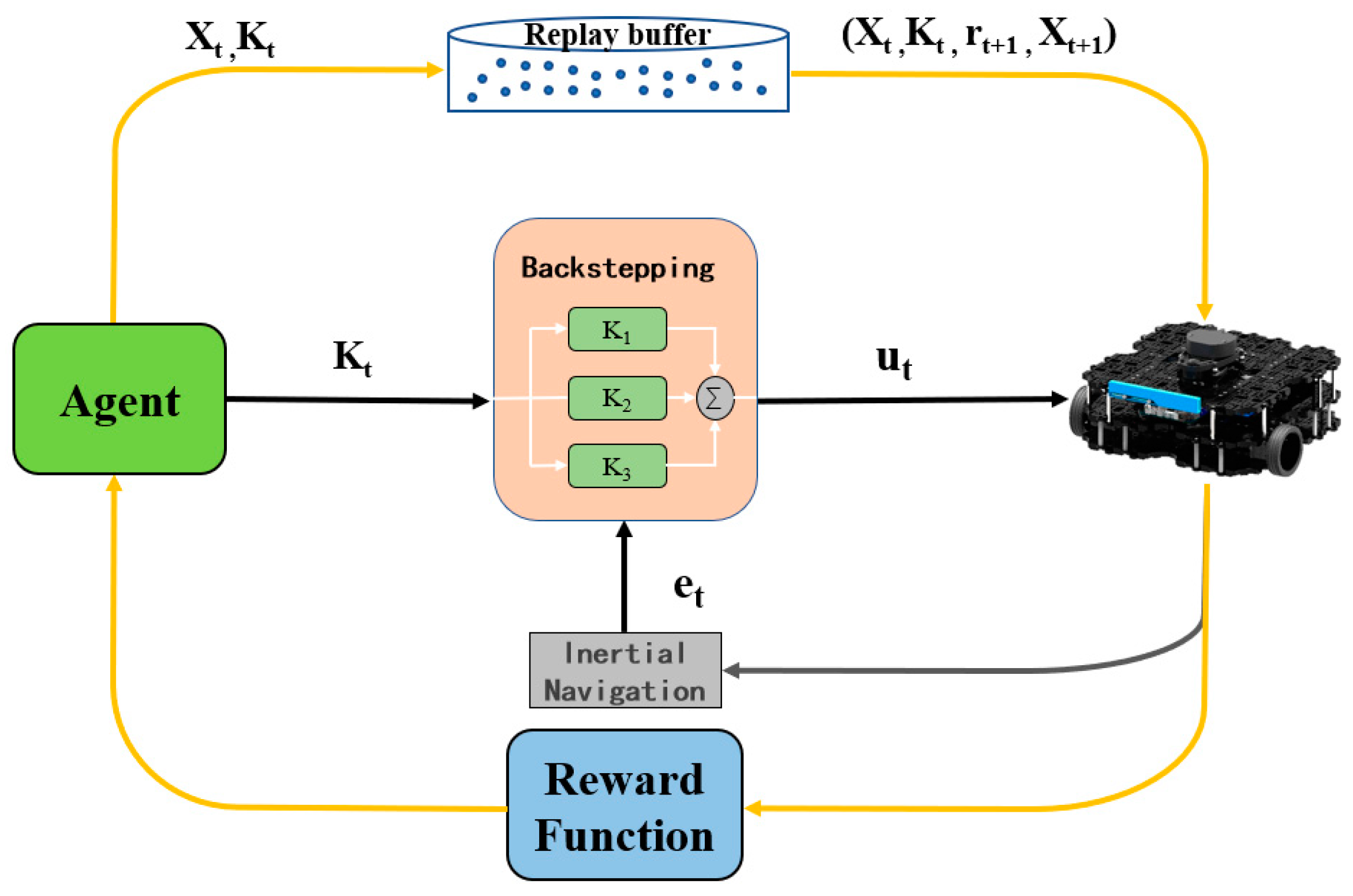As shown in Figure 4, the robot trajectory tracking control structure is designed as follows. In the control structure designed in this paper, the agent RL algorithm plays the role of the upper controller. The system interacts with the environment continuously, and the agent selects and executes the optimal action $k_{\mathrm{t}}$ according to the optimal strategy ${\pi }^{\ast }$. Self-adaptively adjusts the parameter gains of the lower backstepping trajectory tracking controller to achieve high-precision trajectory tracking tasks.

3.1. Experience Replay Mechanism

Mnih [44] et al. proposed the DQN algorithm based on NIPS in the classical field of RL. On the one hand, the deep neural network is used to approximate the action–value function. On the other hand, the experience reply mechanism [45] is used to make the agent significantly improve the utilization rate of samples and the learning efficiency. The experience replay mechanism is a simple and effective method, which stores the data obtained by the interaction between the agent and the environment in the form of memory cells $(x_t,k_t,r_{t+1},x_{t+1})$; it then updates the data according to the random selection of samples in $\mathrm{experience}\mathrm{replay}\mathrm{memory}$. As shown in Figure 5.

This similar experience replay mechanism is common in RL algorithms. It is a model-based RL paradigm structure that repeatedly updates the system model and action-value function in a one-step format. However, this paper is based on the backstepping trajectory tracking error model. We can perform ordered iterations of each algorithm according to the trajectory tracking error model, and we can randomly select batches of minibatch from the replay buffer to transform and update the state-action value function of the system. Moreover, the replay buffer area is bounded, and the maximum amount of system memory unit data it can store is $m$, that is, $R=({\tau }_1,{\tau }_2,{\tau }_3,\dots {\tau }_m)$. If the amount of data stored in the replay buffer area reaches the maximum value, the newly stored memory cells will be overwritten from the side of the first stored memory cells, and cycle in turn.

In this paper, the trajectory tracking controller uses the Double Q-learning algorithm to learn the controller parameter gain adjustment online. Before using the experience replay mechanism, the state–action value functions of $Q_A$ and $Q_B$ need to be randomly initialized. In the daily application of RL algorithms, the initialization of any state-action value function is not a simple and easy task. The establishment of the value function has two advantages for the agent. The first point is that when the value function takes random values, it is crucial in the RL algorithm to facilitate exploration of the unknown areas, and the use of random initialization reduces the possibility of excessive deviation of the state–action value function. The second advantage is that it reduces the number of hyperparameters we input, so algorithm designers do not need expert experience for hyperparameter tuning. The algorithm is friendly to simplify the reproduction of the control algorithm and the ability of cross-platform experiments.

3.2. Incremental Discretization Process

In traditional Q-learning or Double Q-learning algorithms, the state space $\mathbb{X}$ is learned interactively with the environment through uniform discretization. However, our proposed incremental discretization learning algorithm is a process of continuously updating and adding state space $\mathbb{X}$ through interactive learning. With each interaction, the system state is updated according to the two forms of state described in Section 2.2.3. If the system state does not change, an optimal action is selected and executed according to Equation (8), and the same subsequent operation is performed $N$ times. As described in the previous section, in this case, the state of the agent remains unchanged, and the action space $\mathbb{K}$ needs to be incrementally discretized and refined.

We define a tuple, which stores all the information about the state–action of the agent at the current moment, that is, $M_t=(x_t,k_t,l)$. Then, according to the theoretical basis of N-memories, we compare the tuples ${\mathrm{M}}_{\mathrm{t}}$ at each moment, that is ${\mathrm{M}}_{\mathrm{t}}{=\mathrm{M}}_{\mathrm{t}-1}{=\mathrm{M}}_{\mathrm{t}-2}=\dots {=\mathrm{M}}_{\mathrm{t}-\mathrm{n}}$, to determine whether the state–action information of the agent changes during a certain time interval $\mathrm{T}$. 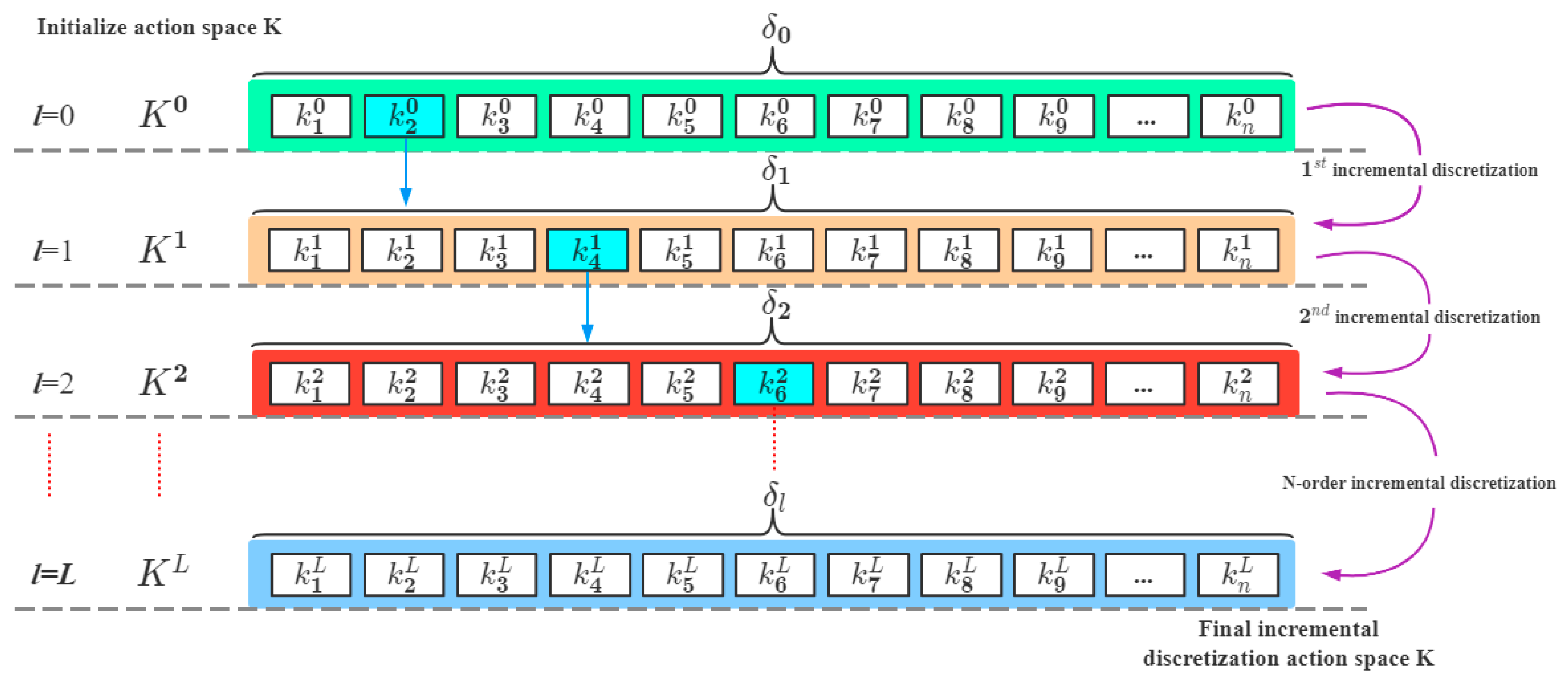If the assumption is valid, the system is in the time interval $\mathrm{T}$ when there is no change. The agent needs to perform incremental discretization processing on the optimal action selected in this time interval to generate a more refined action subset, as shown in Figure 3. Since the state–action space is in one-to-one correspondence, the discretization of the action space will inevitably lead to the discretization of the state space; if the state of the agent is still the same as the current system state at the next moment, the agent will select and execute the optimal action from the newly created subset of actions.

The incremental discretized state-action active learning mechanism avoids the robot’s exploration of unnecessary areas by exploring a given space area, making the state-action space in the Q table more practical. The control accuracy has been transformed from coarse to more refined and accurate, significantly reducing the number of calculations and providing better real-time performance of the control system. As shown in Figure 6, the initialized state space is divided into three regions. This is represented by multiple shaded reachable states, which represent sub-regions of the state space after incremental discretization.

3.3. Algorithmic Statement

The pseudo-code of the proposed incremental Double Q-learning self-adaptive trajectory tracking control algorithm is shown in Algorithm 1. Algorithm 1 pseudo-code of self-adaptive trajectory tracking control algorithm.

Algorithm 1 Double Q-Learning Track Tracking Algorithm Pseudo-Code

1: Input: $\alpha ,\gamma ,r_t,{\epsilon }_0,\mathbb{K},\eta \left(x_t,x_t{}_{+1}\right),l,m,N,\Lambda ,\Delta$

2: Position error of the system at initialization

3: Initializing the experience replay buffer $R$

4: Initializing the state space $\mathbb{X}$

5: Initialize $Q_A$, $Q_B$

6: Loop:

7:    $\epsilon$-Action selection using greedy strategies $k_t$

8:    The current tuple $(x_t,k_t,l)$ is stored in $M_t$

9:    Modelling robot kinematics and calculating positional errors $e_t$

10:    updating→Update Next status $x_{t+1}$, Robot input $u_t$ and reward $r_{t+1}$

11:    if the system is variant then

12:      The current memory cell $(x_t,k_t,r_{t+1},x_{t+1})$ is stored in the experience replay buffer $R$

13:        Divide the region according to the state space $\mathbb{X}$ and find the nearest point of $x_{t+1}$ to $x_i\in \mathbb{X}$

14:        if $x_{t+1}$ is inside $x_i\in \mathbb{X}$ then

15:            if $x_{t+1}$ is in the (0–0.2] interval, there are four chances to update $Q_A$ and $Q_B$

16:            if $x_{t+1}$ is in the (0.2–0.5] interval, there are two chances to update $Q_A$ and $Q_B$

17:            if $x_{t+1}$ is in the (0.5–∞) interval, there are one chance to update $Q_A$ and $Q_B$

18:            else Incorporate $x_{t+1}$ in $\mathbb{X}$ Set up $Q_A$ and $Q_B$ for the newly merged state $x_{t+1}$

19:            end if

20:    else System performs state-action incremental discretization active learning

21:    end if

22:    System startup experience replay mechanism

23:      Update system state $x_t=x_{t+1}$ with incremental discretization $l$.

24: end Loop

In the first line, the hyperparameters of the agent need to be entered. Some of these parameters are common in Q-learning or Double Q-learning. Such as learning rate $\alpha$, reward function $r_t$, discount factor $\gamma$ and exploration strategy ${\epsilon }_0$. There are also some special symbols mentioned in this article. For example, initialize the coarse action space $\mathbb{K}$. Determine the positional relationship between the current system state and the state space according to the value function $\eta \left(x_t,x_t{}_{+1}\right)$. $l$ is the action space discretization level parameter. The size of the minibatch for initializing experience replay is $m$. The parameter $N$ is to determine whether the system is changeable and store the memory unit in $M_t$. Finally, $\Lambda ,\Delta$ represent the threshold sizes of the state space and action space of the agent under different discretization levels.

From line 2 to line 5, initialize the state space $\mathbb{X}$, the experience replay buffer $R$, $Q_A$ and $Q_B$. In this case, the initialization state of the agent is not set randomly; it needs to be measured by some sensors. In this paper, the system’s initial state is the pose measured by the integrated inertial navigation as the initial state $x$.

From line 6 to the end of the loop on line 26, the Double Q-learning incremental discretization active learning algorithm is an infinite loop. First, we use the greedy strategy to select the optimal action in the current state according to $Q_A$ and $Q_B$, then selectively update the value function of $Q_A$ or $Q_B$ according to Equations (9) and (10). Each cycle, update $Q_A$ with the probability of ${\epsilon }_t={\epsilon }_0-\frac{1}{1+e^{-2t}}$ to get the optimal action or update $Q_B$ with the probability of $1-{\epsilon }_t$ to get the optimal action. In line 8, the current state, action and action discretization level of the agent have been combined into a tuple in $M_t$ for subsequent determination of whether the system is changing. In lines 9 and 10, updates the trajectory tracking controller to obtain the robot input $u_t$, the state $x_t{}_{+1}$ at the next moment, and the current reward $r_{t+1}$ according to the pose error and optimal action at the current moment.

After the agent interacts interactively with the environment, it needs to use $M_t$ to determine whether the system has changed. Then, the statements in lines 11 to 24 are executed. When the system changes, this means that the $N$ values stored in $M_t$ are not the same. Therefore, we merge these $N$ memory cells $M_t$ into the experience replay buffer. Then, we find the closest point to $x_t{}_{+1}$ after dividing $x_t{}_{+1}$ in the region of state space $\mathbb{X}$. Update the state–action functions $Q_A$ and $Q_B$ according to the value function $\eta \left(x_t,x_t{}_{+1}\right)$ and the maximum state discretization $\Lambda$. Otherwise, when the system is in the “invariant” condition, the agent can make the robot’s trajectory tracking control accuracy higher through active learning according to the incremental discretization mechanism.

After determining whether the current system has changed, in line 22 uses the experience replay mechanism to update the value functions $Q_A$ and $Q_B$. The agent learning efficiency is faster, and the discretization time is shorter, which significantly reduces the possibility of no convergence in the system. Then, in line 23, update the system’s state and incremental discretization level in preparation for the next cycle.

4. Experimental Result

This section aims to verify the robustness, real-time performance, and anti-disturbance capabilities of the incremental discretization self-adaptive trajectory tracking control algorithm. First, we set the hyperparameters of the proposed control algorithm and verified their performance in the Gazebo. Finally, we will perform experiments to compare the proposed algorithm with Fuzzy-Backstepping trajectory tracking and traditional Backstepping trajectory tracking, adding evidence of the algorithm’s feasibility and effectiveness.

4.1. RL Hyperparameter Settings

Before Gazebo and physical experiments, we must address some common hyperparameter problems in experiments. First, the parameter gain of the self-adaptive trajectory tracking controller is the $k_t=(k_1,k_2,k_3)$ generated by selecting and executing the optimal action of the agent at each moment. In simulation and physical experiments, the initialization of the controller parameter gains is satisfied by the uniform random distribution $U(k_{\min },k_{\max })$. The controller parameter gain $k_t$ is uniformly initialized randomly, reducing the hyperparameter of settings. This simplifies the process of setting hyperparameter for the designer and reduces the reliance on them. By relying less on hyperparameter design, the controller parameters become more refined and can achieve better control accuracy and performance. Moreover, the design of the reward function must provide enough valuable information for the entire system to interact with the environment, without disturbing the external environment. In this paper, the reward function is designed as shown in Equation (11).

$$r_t=-\frac{\ln (1-a(|x_t-x_{ref}|-a))}{a}-a,$$

(11)

where, $a$ is a free parameter, $e_t=|x_t-x_{ref}|$ represents the pose error between the robot’s current position and its desired point. However, when the system’s current pose $x_t$ is close to the desired pose $x_{ref}$, the value of the reward function approaches −1, which indicates that the system is approaching the desired pose. Conversely, the reward function will give a relatively lower reward.

In RL, it is necessary to balance exploration and exploitation in order to learn optimal policies. The balance between exploration and exploitation has a significant impact on the learning of system performance, determining whether the agent uses its existing strategy or explores new strategies. Too much exploration will prevent the agent from getting the maximum reward in the short term, and the agent will randomly choose an action that leads to poor rewards. To address this issue, in the early stages of reinforcement learning, the Q table is randomly initialized, resulting in little information about the interaction between the agent and the environment. To ensure systematic learning, optimal strategy selection, and a comprehensive exploration of the environment, a high exploration strategy is adopted. As the agent gains knowledge over time, the learning process begins and the high-exploration strategy is changed to a lower-exploration strategy [46,47]. To achieve this transition strategy, we use an exploration-exploitation coefficient that decays over time. It determines the probability of the robot system selecting the optimal action based on the current strategy or selecting a random action via the exploration strategy. This probability can be expressed using an equation as follows (12):

$${\rho }_l=-(\frac{({\rho }_{\max }-{\rho }_{\min })}{l_{\max }})l+{\rho }_{\max }.$$

(12)

For the simulation and the physical experiment, the values of ${\epsilon }_0=1$ and ${\epsilon }_1=0.95$ are the same.

4.2. Simulation Experiments

The simulation experiment is composed of two parts: a linear simulation experiment and a circular simulation experiment. In the simulation experiments, the start and end positions of the robot are in the same position, ensuring that the robot’s environment is the same in each experiment.

In the incremental discretization Double Q-learning algorithm, we set the remaining hyperparameters: the learning rate $\alpha =0.2$; discount factor $\gamma =0.95$. The experience replay mechanism also needs to be initialized, we set the initial buffer to $n=7$, and the total is $2^7=128$; we use $N=4$ in N-memories. The incremental discretization levels $l$ for the state space are ${\Lambda }_1=({\rho }_0,{\rho }_1,{\rho }_2,{\rho }_3)$, ${\Lambda }_2=({\rho }_0,{\rho }_1)$, ${\Lambda }_3=({\rho }_0)$. ${\rho }_l=-(\frac{({\rho }_{\max }-{\rho }_{\min })}{l_{\max }})l+{\rho }_{\max }$, where ${\rho }_{\max }=0.25$, ${\rho }_{\min }=0.005$ and $l_{\max }=20$.

To test the feasibility and effectiveness of the algorithm, we conducted simulation experiments using the turtlebot3 in Gazebo, as shown in Figure 7. The robot input has two control variables $u_t=({\nu }_t,{\omega }_t)$, where ${\nu }_{\max }=0.26$ m/s, ${\omega }_{\max }=1.8$ rad/s. In addition, the robot uses a combination of an odometer and slam to filter and locate [48]. The agent state at time $t$ is defined as $x_t=(e_x,e_y,e_{\theta })$, and the initialization of the action state space $k_t$ is randomly selected.

4.2.1. Linear Trajectory Tracking Simulation Experiment

The linear trajectory tracking simulation experiment defines the linear trajectory as shown below in Equation (13).

$$\{\begin{array}{c}y=\nu \times t\times \cos \theta \\ x=\nu \times t\times \sin \theta \end{array}$$

(13)

The initial pose of the robot is ${[x(0),y(0),\theta (0)]}^T={[0,0,\frac{\pi }{4}]}^T$. In the linear simulation, the trajectory tracking target speed is set to $v_c=0.2$ m/s, with an expected angular velocity of ${\omega }_c=0$ rad/s. The initial gains for the Backstepping trajectory tracking controller were chosen to be [0.5, 3.51, 2.5]. The self-adaptive trajectory tracking algorithm based on reinforcement learning is illustrated in Figure 8.

The simulation results of linear trajectory tracking are shown in Figure 8, which comprises six sub-figures. Figure 8a shows the simulated position of linear trajectory tracking. This demonstrates that the proposed adaptive trajectory tracking algorithm is effective, allowing the robot to closely follow the expected trajectory. Figure 8b presents the pose error for the linear trajectory tracking, where the system gradually converges to 0 after about 15 s. Figure 8c illustrates the linear velocity and angular velocity over time for linear trajectory tracking, which stabilize at about 7 s and 8 s, respectively. Figure 8d shows a diagram of the parameter gain effect for the linear trajectory tracking controller. Figure 8e presents a simulation of incremental discretization level for linear trajectory tracking, which reaches the set maximum value over time. Finally, Figure 8f shows the reward value for the linear trajectory tracking that stabilizes around −1.

4.2.2. Circular Trajectory Tracking Simulation Experiment

The circular trajectory tracking simulation experiment defines the circular trajectory as shown below in Equation (14).

$$\{\begin{array}{c}y=r+r\ast \cos (\omega \ast t)\\ x=r\ast \sin (\omega \ast t)\end{array}.$$

(14)

Similar to the linear simulation, the robot’s initial pose is set as ${[x(0),y(0),\theta (0)]}^T={[0,0,\frac{\pi }{3}]}^T$ for the circular simulation. The trajectory tracking target velocity is $v_c=0.2$ m/s, with an expected angular velocity of ${\omega }_c=0.1$ rad/s. The initial gain of the Backstepping trajectory tracking controller is chosen as [0.5, 3.51, 2.5]. The adaptive trajectory tracking algorithm based on reinforcement learning is illustrated in Figure 9.

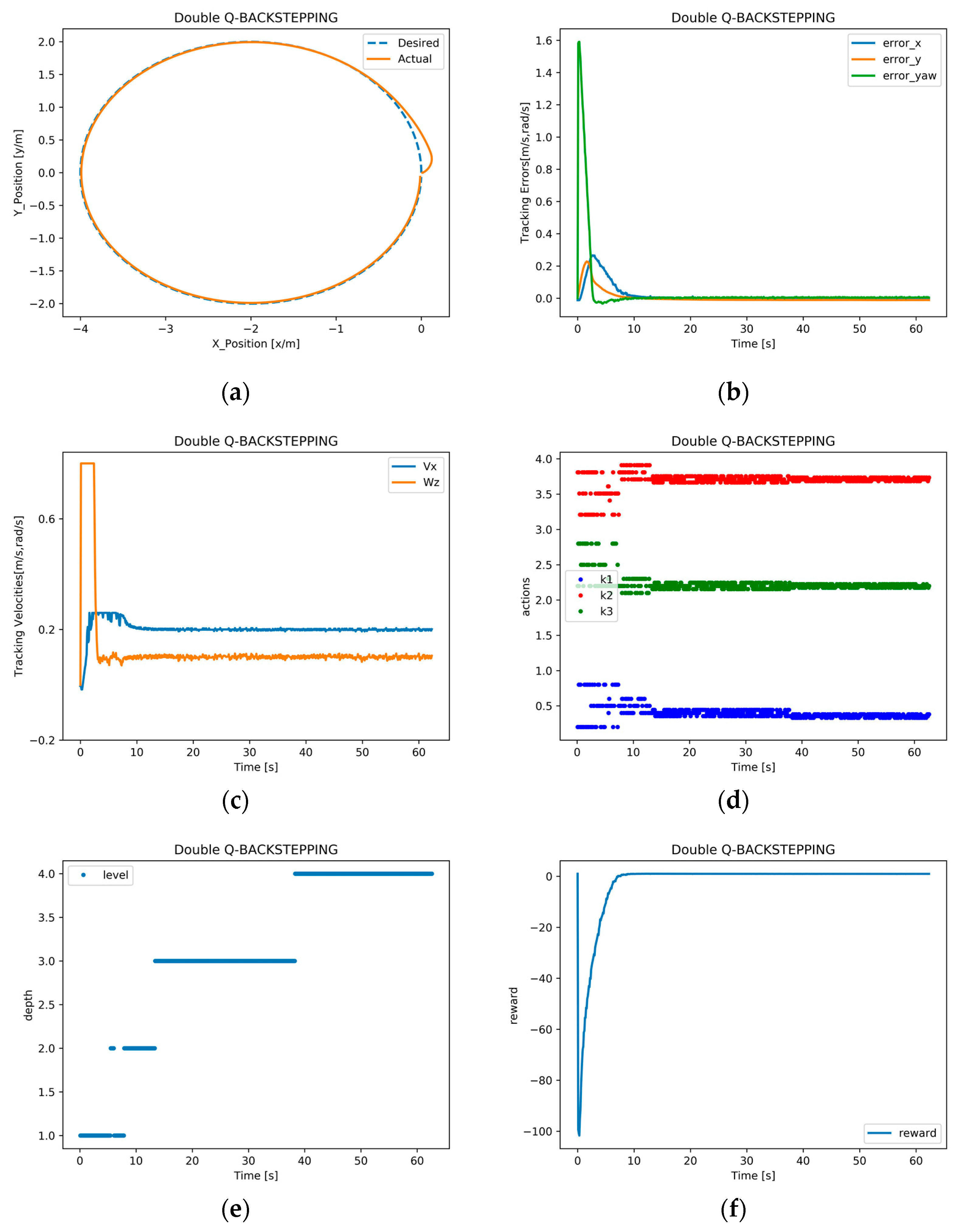
Figure 9 presents the simulation results for circular trajectory tracking. Figure 9a shows the simulated position for circular trajectory tracking, where the trajectory tracking adaptive algorithm proposed in this paper works effectively and allows the robot to closely follow the expected trajectory. Figure 9b displays the pose error for circular trajectory tracking, showing that the system gradually converges to 0 after about 9 s. Figure 9c illustrates the linear velocity and angular velocity over time for circular trajectory tracking, which stabilizes at around 6 s and 5 s, respectively. Figure 9d shows a diagram of the parameter gain effect for the circular trajectory tracking controller, while Figure 9e presents the simulation of incremental discretization level for circular trajectory tracking, which reaches the set maximum value over time. Finally, Figure 9f shows the reward effect diagram for the circular trajectory tracking simulation that stabilizes around −1.

As shown in Figure 8 and Figure 9, the results demonstrate that the designed adaptive trajectory tracking controller can enable the mobile robot system to quickly eliminate disturbance errors and achieve accurate trajectory tracking with high precision.

4.3. Physical Experiments

This subsection will validate an actual mobile robot’s proposed self-adaptive trajectory tracking algorithm. The physical experiment was conducted using the Turtlebot3 Waffle differential mobile robot platform, as shown in Figure 10.

Before beginning the physical experiment, we set the hyperparameters of the RL algorithm and the robot trajectory tracking control system parameters to match those used in the Gazebo environment. The experiment was designed to verify the algorithm’s robustness, adaptability, and anti-disturbance capabilities for the indoor inspection project for mobile robots. In the physical experiment, we verified linear and circular trajectory tracking with a linear velocity of 0.2 m/s.

4.3.1. Physical Experiment with Linear Trajectory Tracking

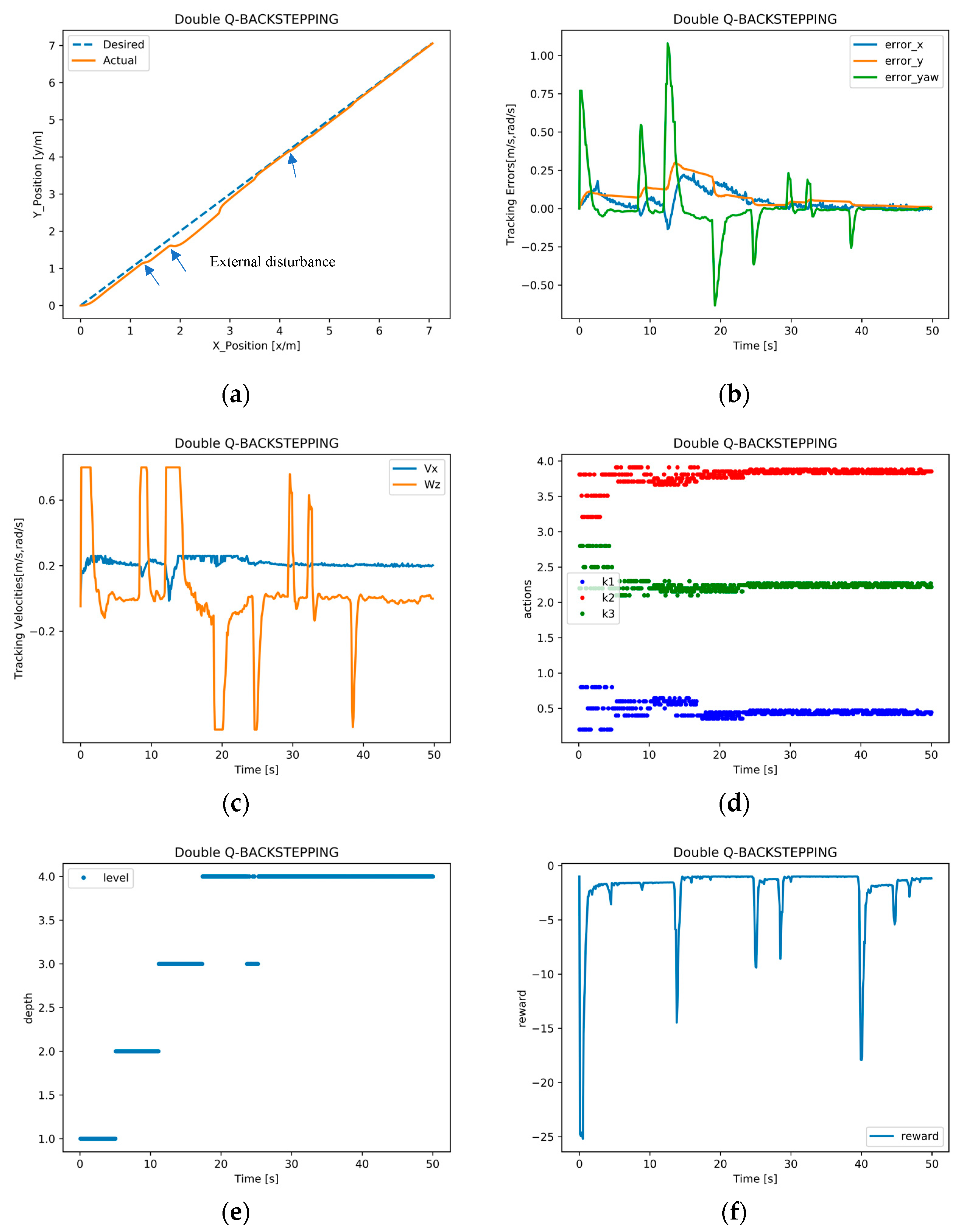
In the linear trajectory tracking experiment, the initial position of the robot is set to ${[x(0),y(0),\theta (0)]}^T={[0,0,\frac{\pi }{4}]}^T$, with an expected velocity of $v=0.2$ m/s and an expected angular velocity of ${\omega }_c=0$ rad/s. The initial gain for the Backstepping trajectory tracking controller was set at [0.5, 3.51, 2.5]. To confirm the adaptiveness and anti-disturbance performance of the trajectory tracking controller, random disturbances were added to test the proposed algorithm’s superior performance. Experiments involving random human disturbance are conducted to verify that even after experiencing communication failure, localization sensor deviation, or mobile robot slippage, the robot can make corrections to the desired trajectory and perform accurate tracking. The linear experiment results based on the double Q-learning adaptive trajectory tracking control algorithm are shown in Figure 11.

To verify the stability, robustness, and anti-interference properties of the adaptive trajectory tracking algorithm, an expected line speed of $v=0.2$ m/s was set for the mobile robot. As seen in Figure 11a, when the system experiences disturbances, the robot can quickly and accurately track the desired trajectory. Figure 11b displays the pose error of the robot while tracking the desired trajectory. The tracking error initially has a large overshoot, but gradually becomes smaller after learning. When the system encounters external disturbances, the error can also rapidly be eliminated, making the system gradually stable. Figure 11c reveals that at around 5 s and 4 s, respectively, the initially assigned linear and angular velocities begin to converge. When the system is disturbed, the robot’s velocity and angular velocity can change swiftly. Figure 11d presents the timetable of the trajectory tracking controller parameter gain over time. Figure 11e illustrates how the system focuses on improving its optimal policies by performing fine discretization operations on the state space and action space through incremental active learning mechanisms. Figure 11f shows how reward changes over time. After the disturbance is eliminated, the reward value finally stabilizes at around −1, demonstrating that the proposed adaptive trajectory tracking controller can achieve accurate curve tracking with good stability, robustness, and anti-interference performance for the mobile robot system.

4.3.2. Physical Experiment with Circular Trajectory Tracking

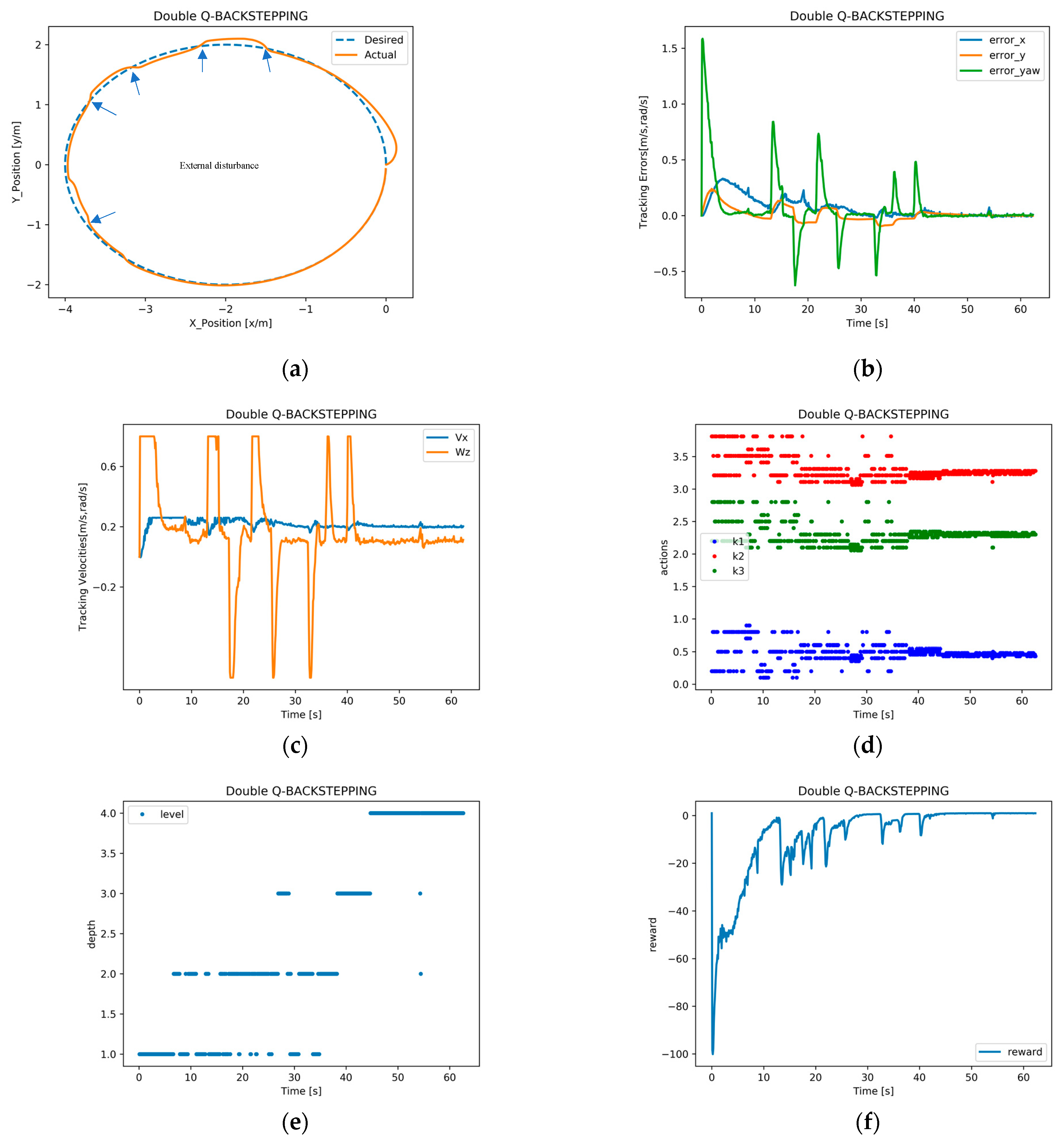
In the circular trajectory tracking experiment, the initial pose of the robot was set to ${[x(0),y(0),\theta (0)]}^T={[0,0,\frac{\pi }{3}]}^T$. The expected velocity and angular velocity were set to $v=0.2$ m/s and ${\omega }_c=0.1$ rad/s, and the initial gain for the Backstepping trajectory tracking controller was set at [0.5, 3.51, 2.5]. Similar to linear trajectory tracking, random perturbations were added to test the superior performance of the proposed algorithm. The results of the circular experiment based on the Double Q-learning adaptive trajectory tracking control algorithm are illustrated in Figure 12.

To evaluate the stability, robustness, and anti-disturbance capabilities of the adaptive trajectory tracking algorithm, we conducted circular trajectory tracking experiments with an expected linear velocity of 0.2 m/s and angular velocity of 0.1 rad/s for the mobile robot. Figure 12a shows that the appearance of system disturbance causes the robot to deviate from the desired trajectory, but the adaptive trajectory tracking algorithm quickly and accurately tracks the desired trajectory. In addition, Figure 12b displays the pose error of the robot during the tracking process, indicating that the tracking error exhibits a large overshoot in the initial stages, but the system gradually stabilizes at about 12 s. When the system experiences external disturbances, the adaptive trajectory tracking controller can rapidly eliminate the error, making the system tend towards a stable state. Figure 12c illustrates that the linear velocity and angular velocity begin to converge around 8 s and 5 s, respectively. Furthermore, when a disturbance occurs, the system quickly adjusts the robot’s velocity and angular velocity. Figure 12d indicates that the optimal trajectory tracking controller parameter gain is obtained after approximately 36 s. Figure 12e shows that as learning progresses, the agent becomes more focused on improving its optimal policy. Through the incremental active learning mechanism, the agent performs fine discretization operations on the state space and action space. Finally, Figure 12f presents the reward values at each moment during the experiments. After eliminating the disturbance, the final reward value is stable at around −1.

As shown in Figure 11 and Figure 12, the results demonstrate that the designed adaptive trajectory tracking controller can enable the mobile robot system to quickly eliminate disturbance errors and achieve accurate trajectory tracking with high precision.

4.4. Comparative Experiments

The traditional backstepping trajectory tracking control algorithm needs to use expert-level prior experience to adjust the controller parameter gain. Therefore, we compare Fuzzy-Backstepping adaptive trajectory tracking controller [49] used in the laboratory robot platform with the advanced Backstepping-Fractional-Older PID controller [50] and the Double Q-learning adaptive trajectory tracking control proposed in this paper. The gains of the trajectory tracking controller selected by the laboratory platform are [5,5,3], $\rho =0$, $\sigma =diag(1,1)$, $e_v^n=\{-0.2,-0.15,-0.1,-0.5,0,0.5,0.1,0.15,0.2\}$, $k_s^n=\{0,0.1,0.2,0.3,0.4\}$, $A_i=\{NB,NM,NS,ZO,PS,PM,PB\}$, $B_i=\{ZO,PS,PM,PB\}$. The gain of the Backstepping-Fractional-Older PID trajectory tracking controller is ${\mathrm{c}}_1=c_2=2$, $\lambda =0.4$, $d_e={\delta }_e=0.95$. 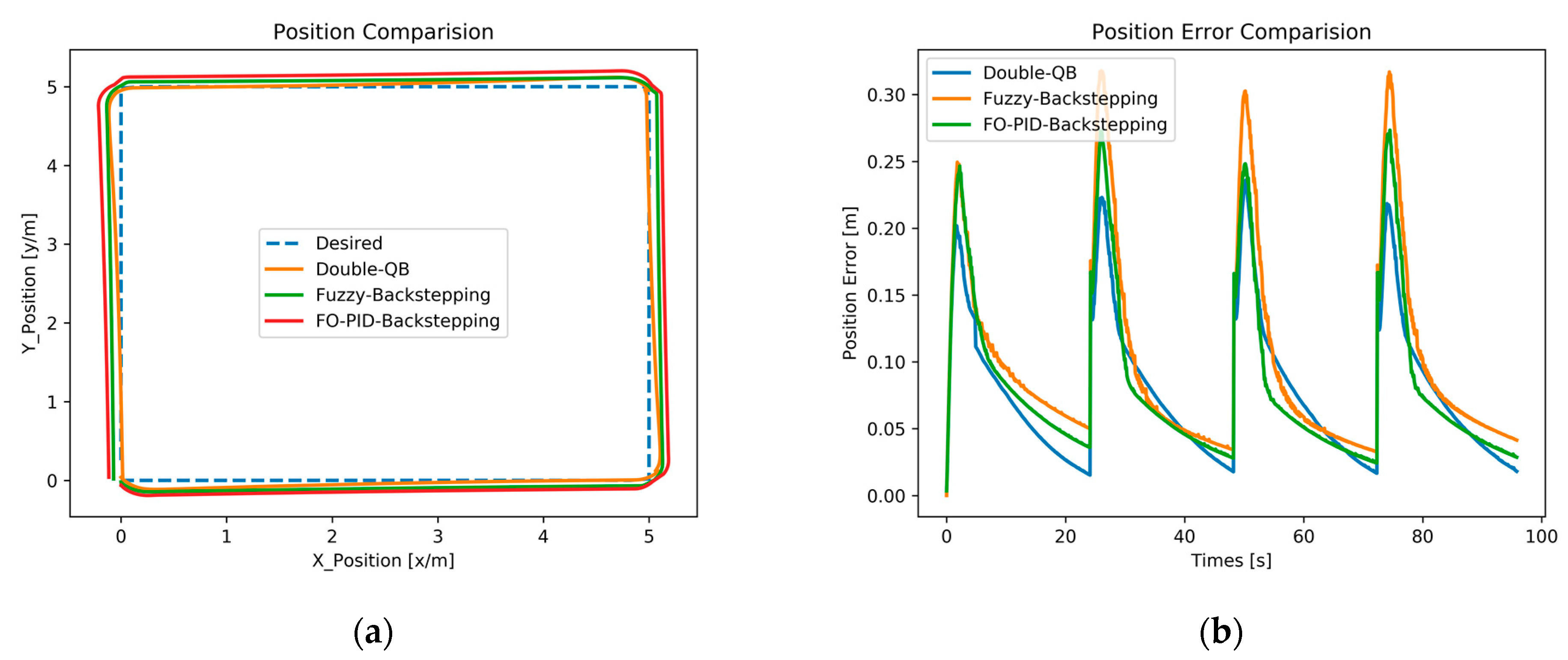Choose the square as the desired trajectory for the actual test, the initial pose of the robot was set to ${[x(0),y(0),\theta (0)]}^T={[0,0,\frac{\pi }{3}]}^T$. The expected velocity and angular velocity were set to $v=0.2$ m/s. The trajectory comparison result is shown in Figure 13a, and the error result is shown in Figure 13b.

Comparing the experimental results, the obtained errors are 0.05 m, 0.08 m, and 0.1 m, respectively. It can be seen that using the algorithm proposed in this paper, the average trajectory tracking error obtained under the same environment and state of the robot is the smallest. In other words, the adaptive trajectory tracking algorithm proposed in this paper demonstrates higher control accuracy and a smaller error under similar conditions in the physical experiment.

5. Conclusions

To address the difficulty of adjusting the parameter gains of the backstepping trajectory tracking controller for mobile robots, this paper proposes an adaptive trajectory tracking control method based on reinforcement learning, according to the characteristics of the backstepping trajectory tracking controller, the double Q-learning learning algorithm and the kinematic model of mobile robots. The improved trajectory tracking online learning algorithm adopts an incremental discrete sub-region fast learning strategy to make the Q-table converge quickly and realize the refinement operation, improving the control accuracy of trajectory tracking. By comparing multiple time memories and experience replay mechanisms, we accelerate both the control learning system and learning process, effectively shortening learning time, so that the optimized algorithm can complete the learning process faster in practical applications and realize the optimal control of trajectory tracking for mobile robots. Finally, the proposed algorithm is verified through both simulation and physical experiments. The experimental results show that the control algorithm can be used to adjust the parameters of the mobile robot trajectory tracking controller online in real time and has good robustness, generalization, real-time, and anti-disturbance capabilities under complex tasks. In addition, we believe that the control algorithm proposed in this paper has broad applicability and can be readily adapted to diverse control systems, such as UAVs, robotic arms, etc.

In future work, we will focus on some interesting topics such as global path planning for mobile robots without SLAM, long-range autonomous navigation, and autonomous obstacle avoidance.