Improved Rotor Flux-Based SMO and RBF-PID Control Strategy for PMSM

Abstract

This paper proposes a control strategy that combines an improved flux-based sliding mode observer with a Radial Basis Function Proportional-Integral-Derivative (RBF-PID) controller for the control of Permanent Magnet Synchronous Motors (PMSM). The strategy aims to address the issues of electrical angle estimation errors and torque fluctuations in traditional sliding mode observer control. The improved sliding mode observer utilizes the flux model of the PMSM to enhance the accuracy of electrical angle estimation, thereby reducing the estimation errors and improving the control of the current loop and speed. The RBF-PID controller ensures system stability while achieving faster response and reduced torque fluctuations. Simulation and experimental results demonstrate that compared to traditional PI control and sliding mode observer control methods, the proposed strategy improves the performance of electrical angle estimation by 7.05% and reduces overshoot in the q-axis current by 28.6%, exhibiting better control performance and smaller errors.

1. Introduction

PMSM is widely used in industrial applications, and obtaining accurate rotor position and speed information is crucial for achieving better control performance. Traditional methods involve installing Hall sensors or encoders to acquire position information, but these approaches are costly and less reliable. To address this issue, many researchers have proposed sensorless control methods based on sliding mode observers [1].

The design of a sliding mode observer relies on the selection of sliding mode gains and switching functions, and numerous scholars, both domestically and internationally, have proposed various methods to optimize traditional sliding mode observers [2,3]. Among them, optimization of the switching function of the sliding mode observer by using a sigmoid function instead of a sign function has been proposed [4], aiming to reduce chattering during sliding surface switching. Based on the rotor flux, the sliding mode observer is a sensorless control method that adaptively adjusts the sliding mode gains [5,6]. It utilizes the characteristics of the rotor flux to design the sliding mode observer for estimating rotor position and speed. In the context of PMSM, scholars have conducted in-depth research and proposed various improved algorithms [7,8,9,10,11] to enhance control accuracy and disturbance rejection capabilities.

In PMSM control, the conventional PID control algorithm has been widely employed. However, due to the nonlinear and coupled characteristics of PMSM, traditional PID control has certain limitations in control performance [12]. Therefore, some scholars have proposed the Radial Basis Function Proportional-Integral-Derivative (RBF-PID) control method to improve control accuracy [13,14,15]. The RBF-PID control method utilizes radial basis functions for nonlinear modeling and optimizes PID control parameters to achieve better control performance [16].

The PMSM control method based on rotor flux sliding mode observer and RBF-PID control offers advantages such as high accuracy and strong disturbance rejection capabilities. Through the optimization and design of various components in the motor control system, high-precision sensorless control of PMSM can be achieved.

2. Build Dynamics Models

The RBF-PID control algorithm combines radial basis function networks with a PID controller to achieve precise control of PMSM. The algorithm consists of three main components: construction of the RBF network, design of the PID controller, and simulation experiments of the control system. By optimizing the control parameters and network structure, this algorithm effectively overcomes issues encountered by PMSM, such as sudden changes in speed and load, thus improving control accuracy and stability.

2.1. Reference Model

The RBF neural network-based PI controller retains the characteristics of traditional PI control and utilizes the self-learning and adaptive capabilities of the RBF neural network to dynamically adjust the parameters of the PI controller in real-time based on the actual operation conditions of the motor. This approach aims to meet the high-performance control requirements of PMSM and enhance system robustness. The RBF network is used to acquire the Jacobian information of the controlled object, which represents the sensitivity of the PMSM control system’s output to the control inputs, and subsequently adjusts the PI parameters.

For the chosen configuration, the RBF neural network has 3 nodes in the input layer, 6 nodes in the hidden layer, and 1 node in the output layer. Gaussian functions are selected as the basis functions. The corresponding neural network structure [17] is illustrated in Figure 1.

The expression for the input layer vector is as follows:

$$X={\left[x_1,x_2,x_3\right]}^T.$$

(1)

The expression for the radial basis vector in the hidden layer of the RBF neural network, denoted as vector h, is as follows:

$$h={\left[h_1,h_2,\dots ,h_6\right]}^T.$$

(2)

The expression for h_i, which represents the radial basis function of the i-th neuron in the hidden layer, is as follows:

$$h_i=\exp \left(-\frac{\Vert X-C_i{\Vert }^2}{2{\sigma }_i^2}\right),i=1,2,\dots ,6.$$

(3)

In the equation, ‖·‖² represents the euclidean norm, also known as the 2-norm. c_i represents the center value vector of the i-th neuron in the hidden layer, and its expression is as follows:

$$C_i={\left[c_{i1},c_{i2},c_{i3}\right]}^T,i=1,2,\dots ,6.$$

(4)

The expression for the basis width vector of the Gaussian function, denoted as σ, is as follows:

$$\sigma ={\left[{\sigma }_1,{\sigma }_2,\dots ,{\sigma }_6\right]}^T.$$

(5)

In the equation, σ_i represents the basis width parameter of the basis function, which is also the variance of the Gaussian function. Therefore, σ_i > 0.

The weight vector from the hidden layer to the output layer, denoted as ω, is as follows:

$$\omega ={\left[{\omega }_1,{\omega }_2,\dots ,{\omega }_6\right]}^T.$$

(6)

From the structure diagram of the RBF neural network, it can be observed that the neural network output y_m(t) at time t is given by:

$$y_m\left(t\right)={\displaystyle \sum _{i=1}^6{\omega }_i\left(t\right)h_i}.$$

(7)

Assuming $y^{*}\left(k\right)$ is the desired output of the RBF neural network, the performance index J(k) of the neural network can be obtained from the desired output and the actual output, as shown below:

$$J\left(k\right)=\frac{1}{2}{\left(y^{*}\left(k\right)-y_m\left(k\right)\right)}^2.$$

(8)

Afterward, the gradient descent method is used to update the center points, basis width parameters, and weights of the radial basis functions.

According to the chain rule of partial derivatives, it can be determined that

$$\frac{\partial J\left(k\right)}{\partial {\omega }_i\left(k\right)}=\frac{\partial J\left(k\right)}{\partial y_m\left(k\right)}·\frac{\partial y_m\left(k\right)}{\partial {\omega }_i\left(k\right)}.$$

(9)

Therefore, the updated equation for the weight ω_i(k) is as follows:

$$\frac{\partial J\left(k\right)}{\partial {\omega }_i\left(k\right)}=\frac{\partial \left(\frac{1}{2}{\left(y^{*}\left(k\right)-y_m\left(k\right)\right)}^2\right)}{\partial y_m\left(k\right)}·\frac{\partial y_m\left(k\right)}{\partial {\omega }_i\left(k\right)}=-\left(y^{*}\left(k\right)-y_m\left(k\right)\right)\frac{\partial y_m\left(k\right)}{\partial {\omega }_i\left(k\right)}.$$

(10)

In the Formula (10), the $\frac{\partial y_m\left(k\right)}{\partial {\omega }_i\left(k\right)}$ can be expressed as

$$\frac{\partial y_m\left(k\right)}{\partial {\omega }_i\left(k\right)}=\frac{\partial \left({\displaystyle \sum _{j=1}^6{\omega }_j\left(k\right)h_j}\right)}{\partial {\omega }_i\left(k\right)}=h_i.$$

(11)

Therefore, combining Formulas (10) and (11), it can be concluded:

$$\frac{\partial J\left(k\right)}{\partial {\omega }_i\left(k\right)}=-\left(y^{*}\left(k\right)-y_m\left(k\right)\right)h_i.$$

(12)

By modifying $\frac{\partial J\left(k\right)}{\partial {\omega }_i\left(k\right)}$, we obtain $\Delta {\omega }_i\left(k\right)$, which is expressed as follows:

$$\Delta {\omega }_i\left(k\right)=-\eta \frac{\partial J\left(k\right)}{\partial {\omega }_i\left(k\right)}=\eta \left(y^{*}\left(k\right)-y_m\left(k\right)\right)h_i.$$

(13)

In Formula (13), $\eta$ represents the learning rate.

Because the RBF neural network may get trapped in local minima during computation, adding a dynamic factor component during the weight update process can prevent the RBF from converging to a minimum. Therefore, the expression for the dynamic factor component is as follows:

$$\Delta {\omega }_i\left(k-1\right)=\alpha \left({\omega }_i\left(k-1\right)-{\omega }_i\left(k-2\right)\right).$$

(14)

Formula (14) $\alpha$ represents the dynamic factor.

Therefore, the updated equation for the weight ${\omega }_i\left(k\right)$ is as follows:

$${\omega }_i\left(k\right)=\omega \left(k-1\right)+\eta \left(y^{*}\left(k\right)-y_m\left(k\right)\right)h_i+\alpha \left({\omega }_i\left(k-1\right)-{\omega }_i\left(k-2\right)\right).$$

(15)

Similarly, the update expressions for the basis width parameter ${\sigma }_i\left(k\right)$ and the center points of the basis functions $c_{ij}\left(k\right)$ can be obtained as follows:

$$\left\{\begin{array}{c}{\sigma }_i\left(k\right)={\sigma }_i\left(k-1\right)+\eta \left(y^{*}\left(k\right)-y_m\left(k\right)\right)\frac{{\omega }_i\left(k\right)·\left|\right|X-C_i{\left|\right|}^2·h_i}{{\sigma }_k^3\left(k\right)}+\alpha \left({\sigma }_i\left(k-1\right)-{\sigma }_i\left(k-2\right)\right),\hfill \\ c_{ij}\left(k\right)=c_{ij}\left(k-1\right)+\eta \left(y^{*}\left(k\right)-y_m\left(k\right)\right)\frac{{\omega }_i\left(k\right)·\left(x_i-c_{ij}\left(k\right)\right)·h_i}{{\sigma }_k^2\left(k\right)}+\alpha \left(c_{ij}\left(k-1\right)-c_{ij}\left(k-2\right)\right).\hfill \end{array}\right.$$

(16)

2.2. Design of RBF-PID Parameter Tuning Algorithm

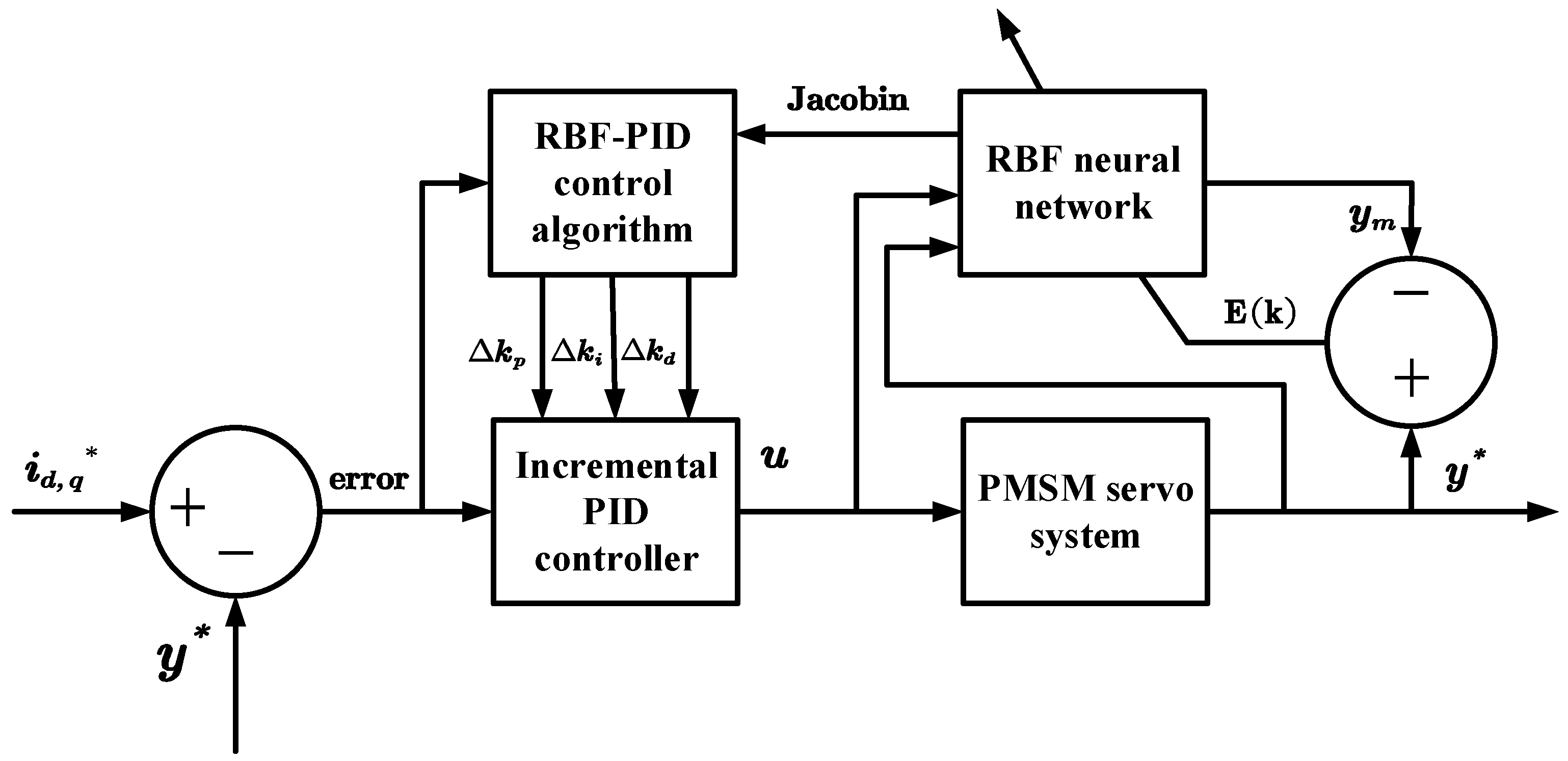
In order to achieve better control performance, it is necessary to adjust the parameters of the PID controller, as there are multiple parameters involved. In this paper, an RBF-PID parameter tuning algorithm is proposed by combining the RBF neural network as an optimization tool with traditional parameter tuning methods. This algorithm introduces the RBF neural network, where the parameters of the controller are treated as the network’s outputs, and the system’s control error is used as the input. By leveraging the nonlinear mapping capability of the neural network, the parameters are optimized to achieve adaptive tuning of the controller’s parameters. This algorithm combines the advantages of traditional PID controllers and RBF neural networks, effectively improving the control accuracy and robustness of the control system. Figure 2 illustrates the structure of the RBF-PID controller.

The control error of the incremental PID controller used in this paper is defined as follows:

$$error\left(k\right)=i_{d,q}^{*}-y^{*}\left(k\right).$$

(17)

In Formula (17), $i_{d,q}^{*}$ represents the desired d-axis and q-axis currents while $y^{*}\left(k\right)$ represents the feedback current.

The performance index for RBF neural network tuning is defined as follows:

$$E\left(k\right)=\frac{1}{2}erro{r}^2\left(k\right).$$

(18)

According to the algorithm of the incremental PID controller, the controller input is given by the following expression:

$$\{\begin{array}{l}{x}_i\left(1\right)=error\left(k\right)-error\left(k-1\right),\hfill \\ x_i\left(2\right)=error\left(k\right),\hfill \\ x_i\left(3\right)=error\left(k\right)-2error\left(k-1\right)+error\left(k-2\right).\hfill \end{array}$$

(19)

Similarly, the controller output is given by the following expression:

$$u\left(k\right)=u\left(k-1\right)+\Delta u\left(k\right).$$

(20)

In Formula (20), $u\left(k\right)$ represents the output of the PID controller at time step k, $u\left(k-1\right)$ represents the output of the PID controller at time step k − 1, and $\Delta u\left(k\right)$ represents the increment of the PID controller output between time step k − 1 and k.

According to the algorithm of the incremental PID controller:

$$\Delta u\left(k\right)=k_p{x}_i\left(1\right)+k_i{x}_i\left(2\right)+k_d{x}_i\left(3\right).$$

(21)

Similarly, by using the gradient descent method, the adjustment amounts can be obtained as follows:

$$\left\{\begin{array}{c}\Delta k_p=-\eta \frac{\partial E\left(k\right)}{\partial y_m\left(k\right)}\frac{\partial y_m\left(k\right)}{\partial \Delta u\left(k\right)}\frac{\partial \Delta u\left(k\right)}{\partial k_p}=\eta e\left(k\right)\frac{y_m\left(k\right)}{\partial \Delta u\left(k\right)}{x}_i\left(1\right),\hfill \\ \Delta k_i=-\eta \frac{\partial E\left(k\right)}{\partial y_m\left(k\right)}\frac{\partial y_m\left(k\right)}{\partial \Delta u\left(k\right)}\frac{\partial \Delta u\left(k\right)}{\partial k_i}=\eta e\left(k\right)\frac{y_m\left(k\right)}{\partial \Delta u\left(k\right)}{x}_i\left(2\right),\hfill \\ \Delta k_d=-\eta \frac{\partial E\left(k\right)}{\partial y_m\left(k\right)}\frac{\partial y_m\left(k\right)}{\partial \Delta u\left(k\right)}\frac{\partial \Delta u\left(k\right)}{\partial k_d}=\eta e\left(k\right)\frac{y_m\left(k\right)}{\partial \Delta u\left(k\right)}{x}_i\left(3\right).\hfill \end{array}\right.$$

(22)

The $\frac{\partial y_m\left(k\right)}{\partial \Delta u\left(k\right)}$ represents the Jacobian information of the controlled object, which can be identified through the RBF neural network as follows:

$$\frac{\partial y_m\left(k\right)}{\partial \Delta u\left(k\right)}={\displaystyle \sum _{j=1}^6{\omega }_j{h}_j\frac{c_j-\Delta u\left(k\right)}{2{\sigma }_j^2}}.$$

(23)

By identifying through the RBF neural network, the system error $E\left(k\right)$ is consistently maintained at the optimal error level, resulting in improved system accuracy and robust stability compared to the traditional PI control.

3. Design of Improved Rotor Flux-Based Sliding Mode Observer

This section may be divided into subheadings. It should provide a concise and precise description of the experimental results, their interpretation, as well as the experimental conclusions that can be drawn.

According to the traditional sliding mode observer, we can obtain the current state equations in $\alpha -\beta$ of the two-phase stationary coordinate system as follows [18]:

$$\{\begin{array}{l}\frac{d{i}_{\alpha }}{dt}=-\frac{R_s}{L_s}{i}_{\alpha }+\frac{1}{L_s}{u}_{\alpha }-\frac{1}{L_s}{e}_{\alpha },\hfill \\ \frac{d{i}_{\beta }}{dt}=-\frac{R_s}{L_s}{i}_{\beta }+\frac{1}{L_s}{u}_{\beta }-\frac{1}{L_s}{e}_{\beta }.\hfill \end{array}$$

(24)

In Formula (24): $i_{\alpha }{i}_{\beta }$ represents the current component in the stator $\alpha ,\beta$-axis; represents the voltage component in the stator $\alpha ,\beta$-axis; $e_{\alpha },e_{\beta }$ represents the back electromotive force (EMF) component in the stator $\alpha ,\beta$-axis; $R_s,L_s$ represents the stator resistance and stator inductance of the motor.

The back electromotive force equation [19] is as follows:

$$\{\begin{array}{l}{e}_{\alpha }=-{\omega }_e{\psi }_f\sin {\theta }_e,\hfill \\ e_{\beta }={\omega }_e{\psi }_f\cos {\theta }_e.\hfill \end{array}$$

(25)

In Formula (25): ${\omega }_e$ represents the electrical angular velocity of the motor rotor; ${\psi }_f$ represents the magnetic flux of the permanent magnet; ${\theta }_e$ represents the electrical angular position of the motor rotor relative to the $\alpha$-axis.

A sigmoid function with variable boundary layer thickness is introduced to reduce chattering to replace the traditional saturation function. The dynamic equation of the current error for the sliding-mode observer based on the sigmoid function [20] is as follows:

$$\{\begin{array}{l}\frac{d\left({\widehat{i}}_{\alpha }-i_{\alpha }\right)}{dt}=-R_s\frac{\left({\widehat{i}}_{\alpha }-i_{\alpha }\right)}{L_s}+\frac{e_{\alpha }}{L_s}-\frac{kG\left({\widehat{i}}_{\alpha }-i_{\alpha }\right)}{L_s},\hfill \\ \frac{d\left({\widehat{i}}_{\alpha }-i_{\beta }\right)}{dt}=-R_s\frac{\left({\widehat{i}}_{\beta }-i_{\beta }\right)}{L_s}+\frac{e_{\beta }}{L_s}-\frac{kG\left({\widehat{i}}_{\beta }-i_{\beta }\right)}{L_s}.\hfill \end{array}$$

(26)

The $G\left(x\right)$ is the sigmoid function, with the specific expression given as follows:

$$G\left(x\right)=\frac{1-e^{-ax}}{1+e^{-ax}}.$$

(27)

For further analysis of this sliding mode observer, if there exists a stable sliding mode, that is when $t\to +\infty$ equals $s\left(t\right)=0$, the Lyapunov function is defined as follows:

$$V=\frac{1}{2}{S}^T·S.$$

(28)

The $S={\left[s_{\alpha }{s}_{\beta }\right]}^T={\left[\overline{i_{\alpha }}\overline{i_{\beta }}\right]}^T={\left[{\widehat{i}}_{\alpha }-i_{\alpha }{\widehat{i}}_{\beta }-i_{\beta }\right]}^T$ represents a certain condition.

Taking the derivative of the Lyapunov function, we have

$$\dot{V}=S^T·\dot{S}=-\frac{R_s}{L_s}\left(s_{\alpha }^2+s_{\beta }^2\right)+\frac{1}{L_s}\left(e_{\alpha }·s_{\alpha }+e_{\beta }·s_{\beta }\right)-\frac{k}{L_s}\left(G\left(s_{\alpha }\right)·s_{\alpha }+G\left(s_{\beta }\right)·s_{\beta }\right).$$

(29)

According to the second theorem of Lyapunov, the sliding mode observer tends to stability when $\dot{V}\le 0$ satisfying the following conditions:

$$k>\frac{\max \left(\left|e_{\alpha }\right|,\left|e_{\beta }\right|\right)}{\left|G\left(s_{\alpha ,\beta }\right)\right|}.$$

(30)

when the sliding mode observer reaches a stable state, the sliding mode exists, and the system can reach the sliding surface and achieve asymptotic stability. Combining Formulas (25) and (30), the sliding mode gain of the observer can be determined as follows:

$$k=\left|{\omega }_e\right|·{\psi }_f.$$

(31)

Therefore, the selection of the sliding mode gain is proportional to the electrical angle, and it also varies with the change in speed. The sliding mode observer can adaptively adjust to reduce chattering. As for the selection of the slope parameter a in the sigmoid function, the following analysis can be conducted.

When $s_{\alpha ,\beta }$ is within the boundary layer and the system is in a steady state, when:

$$\dot{S}={\left[{\dot{s}}_{\alpha } {\dot{s}}_{\beta }\right]}^T=0.$$

(32)

According to Formula (26), it can be seen that

$$\{\begin{array}{l}{\dot{s}}_{\alpha }=-\frac{R_s}{L_s}·s_{\alpha }+\frac{e_{\alpha }}{L_s}-\frac{k\left(1-e^{-a{s}_{\alpha }}\right)}{L_s\left(1+e^{-a{s}_{\alpha }}\right)}=0,\hfill \\ {\dot{s}}_{\beta }=-\frac{R_s}{L_s}·s_{\beta }+\frac{e_{\beta }}{L_s}-\frac{k\left(1-e^{-a{s}_{\beta }}\right)}{L_s\left(1+e^{-a{s}_{\beta }}\right)}=0.\hfill \end{array}$$

(33)

Therefore, according to the above equation, the slope parameter a of the sigmoid function is given by

$$a=\frac{1}{s_{\alpha ,\beta }}·\ln \left(\frac{e_{\alpha ,\beta }-R_s{s}_{\alpha ,\beta }+k}{k-e_{\alpha ,\beta }+R_s{s}_{\alpha ,\beta }}\right).$$

(34)

In Formula (34), “a” represents the slope of the sigmoid function.

The current observation error boundary layer width is influenced by the adjustable slope. While using a smaller adjustable slope can attenuate the inherent chattering of sliding mode observations, it can also result in a larger observation error in the boundary layer. In the context of traditional exponential convergence rates, the adjustable slope “a” can yield the most suitable adjustable parameters once the electrical parameters are determined. This approach not only reduces chattering in sliding mode observations but also takes into account the observation error in the boundary layer, achieving a more accurate electrical angle observation for the motor.

Based on the above analysis, once the back electromotive force, current error, and sliding mode gain coefficient are determined, the slope of the sigmoid function can be uniquely determined.

For the sliding mode observer in a zero-speed state, the electrical angular velocity of the rotor tends to be zero. In this case, it is necessary to introduce a zero-speed offset term to ensure that the sliding mode gain coefficient is non-zero at a zero-speed state. This can be expressed by the following equation:

$$ϵ=\left|{\omega }_e\right|{\psi }_f+\varsigma .$$

(35)

In Formula (35), $\varsigma$ represents the offset term when the motor is at zero speed. The corresponding current observer becomes

$$\left\{\begin{array}{c}\frac{d{\widehat{i}}_{\alpha }}{dt}=-\frac{R_s}{L_s}{\widehat{i}}_{\alpha }+\frac{u_{\alpha }}{L_s}-\frac{ϵ}{L_s}G\left(s_{\alpha }\right),\hfill \\ \frac{d{\widehat{i}}_{\beta }}{dt}=-\frac{R_s}{L_s}{\widehat{i}}_{\beta }+\frac{u_{\beta }}{L_s}-\frac{ϵ}{L_s}G\left(s_{\beta }\right).\hfill \end{array}\right.$$

(36)

The corresponding estimated back electromotive force is given by

$$\{\begin{array}{l}{\widehat{e}}_{\alpha }=ϵ·G\left(s_{\alpha }\right),\hfill \\ {\widehat{e}}_{\beta }=ϵ·G\left(s_{\beta }\right).\hfill \end{array}$$

(37)

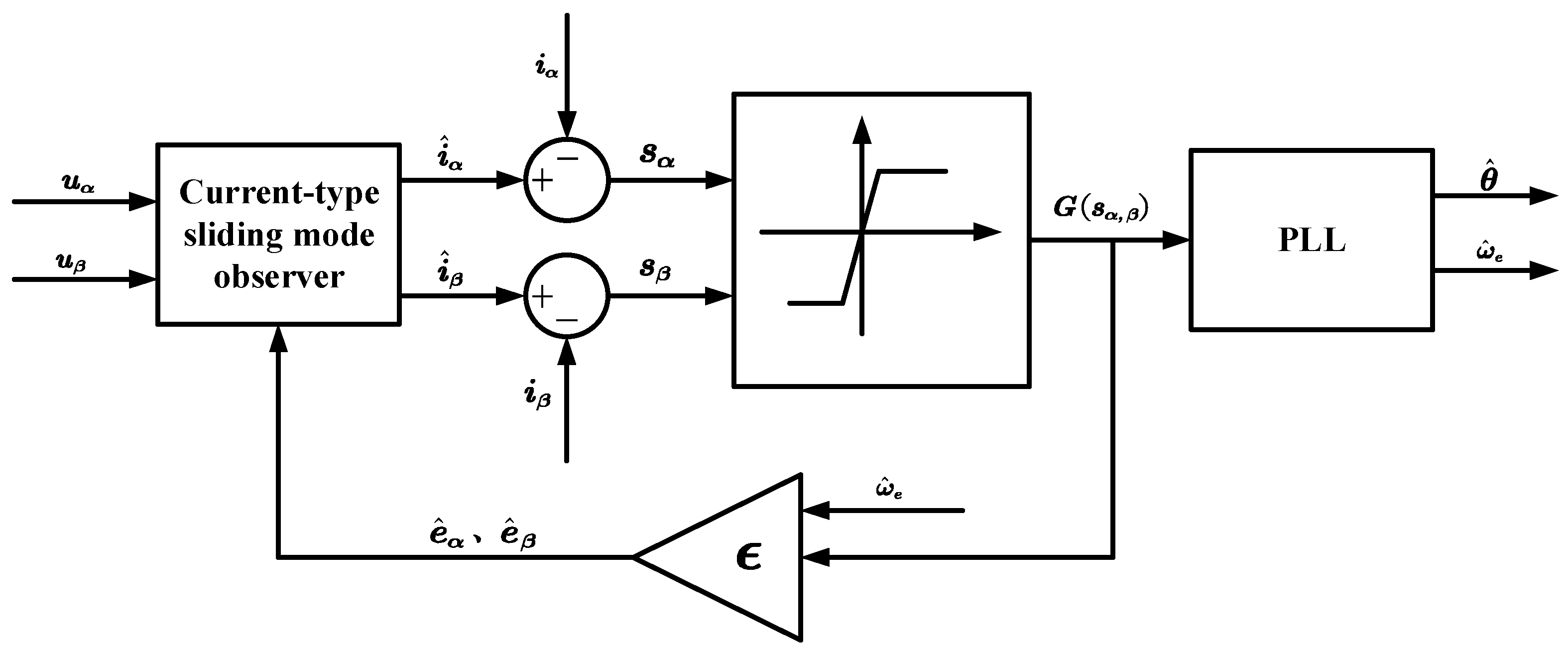
According to the above analysis, the improved sliding mode observer performs position estimation based on the parameter $G\left(s_{\alpha ,\beta }\right)$. The specific estimation process is as follows:

$$\left[\begin{array}{c}G\left(s_{\alpha }\right)\\ G\left(s_{\beta }\right)\end{array}\right]=\frac{{\psi }_f{\widehat{\omega }}_e}{ϵ}\left[\begin{array}{c}-\sin {\widehat{\theta }}_e\\ \cos {\widehat{\theta }}_e\end{array}\right].$$

(38)

The system block diagram of the improved sliding mode observer is shown in Figure 3 as follows:

The improved rotor flux-based SMO provides significant improvements in the estimation of rotor electrical angle and speed compared to the traditional SMO method.

4. Simulation Analysis

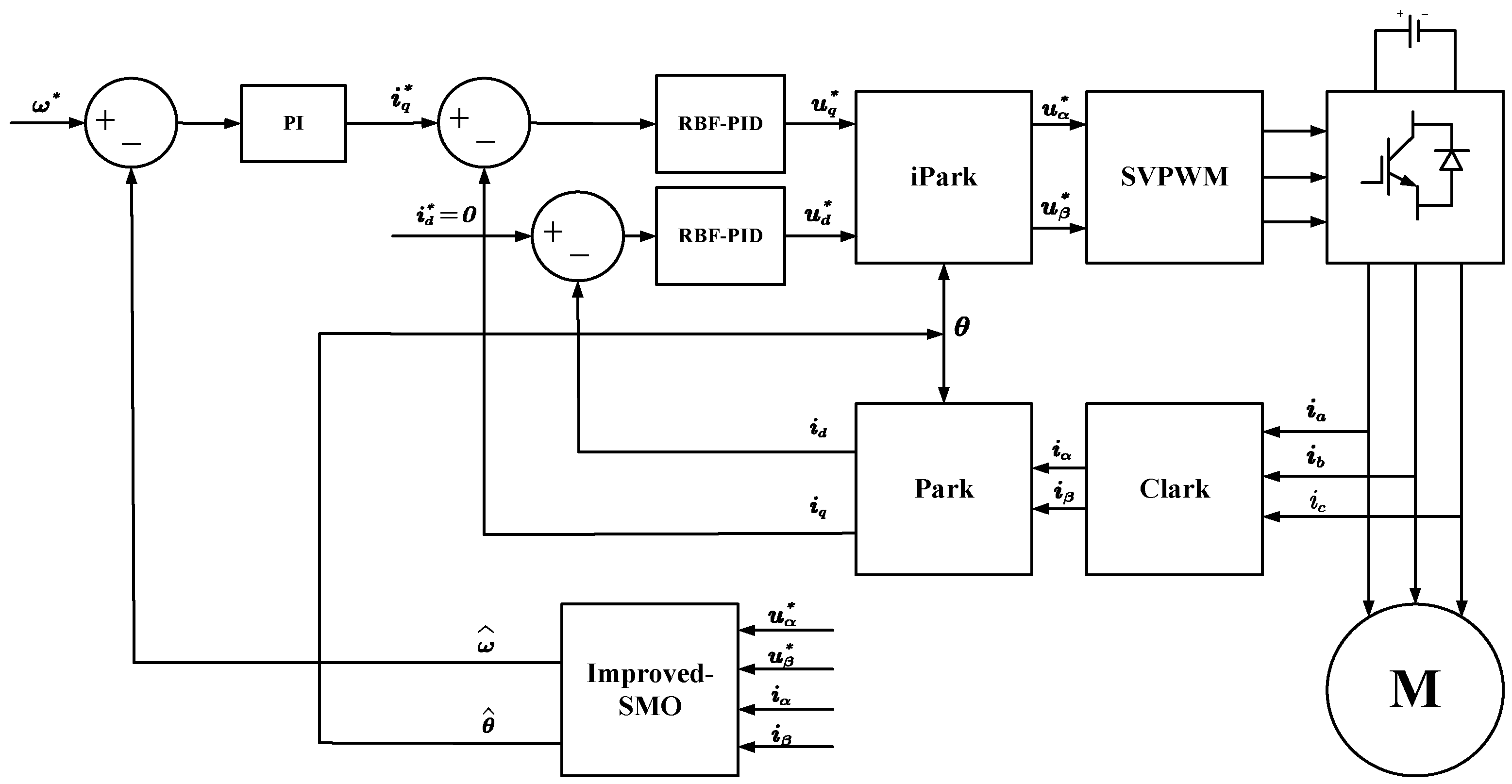
The schematic diagram of the PMSM speed control system using RBF-PID as the speed controller and the improved SMO based on the rotor flux model is shown in Figure 4 below:

To validate the control effectiveness of the algorithm, this study conducted simulation verification using Matlab/Simulink. The main parameters for the simulation experiment are shown in

Table 1. Simulation experiment parameters.

The Name of the Parameter	The Reference Value	Unit
Rated line voltage	220	V
Rated line current	3	A
Rated power	750	W
Rated speed	3000	r/min
Stator phase resistance	0.045	Ω
Inductance	0.235	mH
Permanent magnet flux linkage	0.048517	Wb
Polar	4	/
Learning rate in RBF-NN	0.4	/

below.

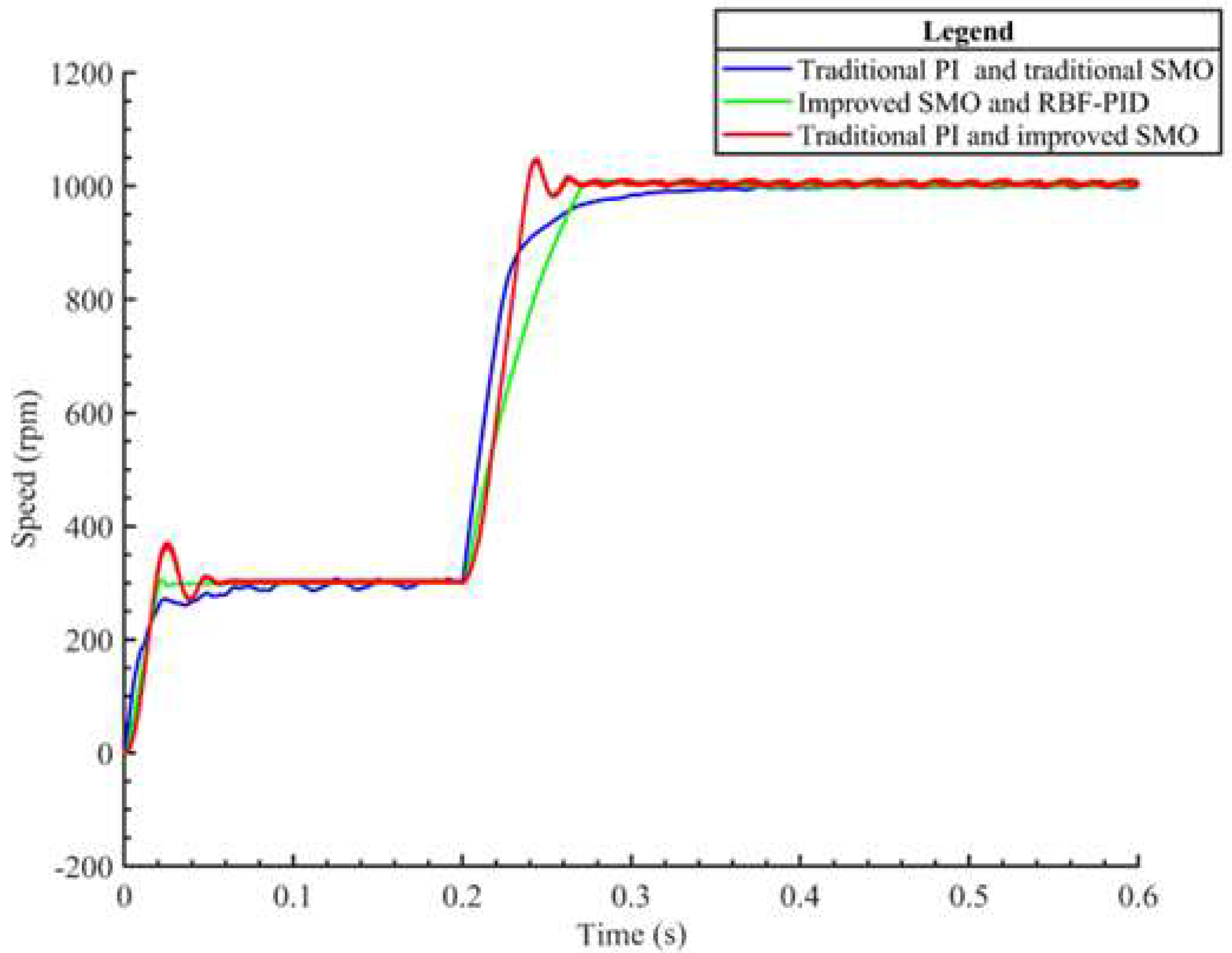
Figure 5 shows the speed response curves under the control of traditional PI with traditional SMO, RBF-PID with improved rotor flux-based sliding mode observer, and improved SMO with traditional PI strategies. The simulation time is 0.6 s, with an initial given speed of 300 r/min, and the speed suddenly changes to 1000 r/min at 0.3 s. From Figure 5, it can be observed that when using traditional PI and traditional SMO for control at low speeds, the SMO speed estimation is inaccurate and exhibits oscillations. When the speed changes to high speed, the response speed of traditional PI is slow. Under the control of improved SMO and traditional PI, although the speed estimated by the improved SMO is relatively stable compared to the traditional method at both low and high speeds, there is still a significant overshoot at the moment of speed mutation. Under the control of improved SMO and RBF-PID, compared to the previous two control strategies, the speed estimation is more stable at both low and high-speed operating conditions, and only a small overshoot is present during speed mutation. The control effect is more ideal compared to the previous two strategies.

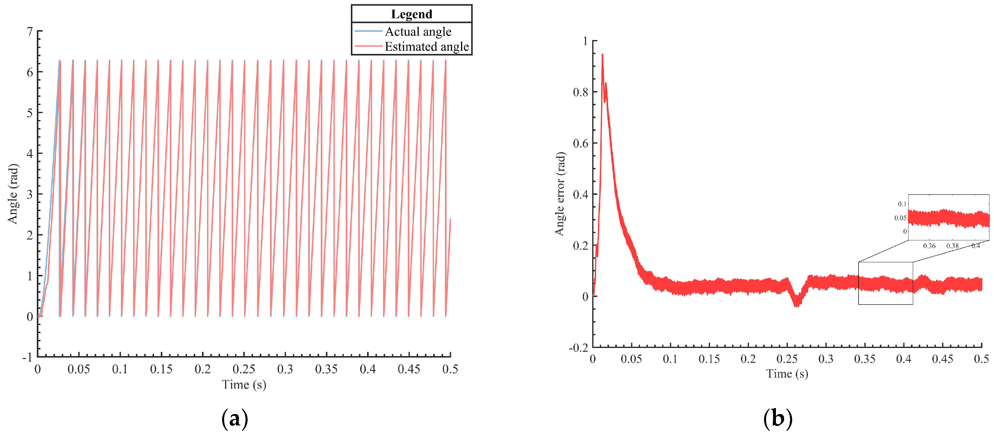
Figure 6a,b show the tracking curves of the rotor angle and the angle error, respectively, under the control of the RBF-PID controller and traditional sliding mode observer. The simulation time is 0.5 s, with a given speed of 1000 r/min, and a torque of 3 Nm is applied at 0.25 s. From Figure 6a, it can be observed that when using the traditional sliding mode observer and RBF-PID controller for control, there is a certain error in the tracking curve of the motor rotor angle during the acceleration phase, with a maximum error of up to 0.9 rad. However, the overall tracking effect is relatively satisfactory, as the estimated rotor angle curve and the estimated rotor angle curve in the tracking curve roughly overlap. From Figure 6b, it can be seen that the error control is effective when sudden loading occurs, with the error being controlled within −0.15 rad. However, there is still room for further optimization in the rotor angle control effect, especially in the tracking effect during the initial angle and sudden loading.

Figure 7a,b illustrate the rotor angle tracking curves and error curves of the motor under the control of the improved rotor flux-based sliding mode observer (SMO) and RBF-PID controller strategy. In Figure 7a, it can be observed that during the acceleration phase, the improved control strategy exhibits a more desirable rotor angle tracking performance compared to the traditional strategy, with the tracking error decreasing from 0.9 rad to 0.66 rad. The actual rotor angle closely follows the estimated rotor angle curve. Figure 7b demonstrates that the improved control strategy achieves better control performance with an error controlled within −0.05 rad. Overall, the adoption of the improved SMO and RBF-PID controller strategy enhances the accuracy of rotor angle estimation, particularly during startup, leading to improved tracking performance.

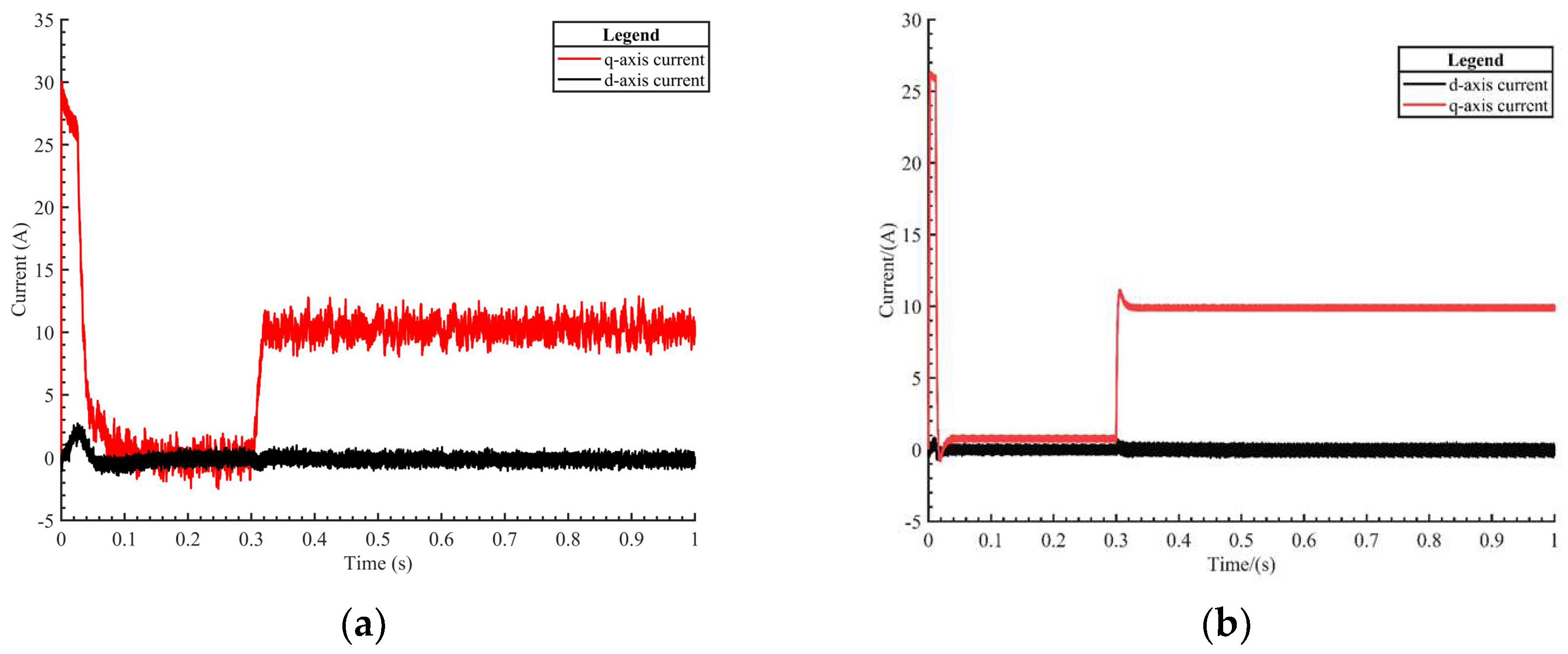
Figure 8a,b show the response curves of the d-q axis currents under the control of RBF-PID with improved SMO and traditional PI with traditional SMO, respectively, under the control of. The simulation time is 1 s, and the desired speed is set to 1000 r/min. A torque of 10 is applied at 0.3 s.

Figure 8a shows that during motor startup, the q-axis current undergoes a significant abrupt change, reaching a maximum of 30 A. This indicates a poor control effect and significant torque ripple during motor startup. After the load is applied, there is approximately 2 A of current oscillation in the q-axis, which is not ideal for motor current control. Therefore, further optimization can be done to improve the current control effect during motor startup.

Figure 8b shows that during motor startup, the q-axis current undergoes a reduced abrupt change compared to traditional SMO and traditional PI, reaching 26 A. The torque ripple is effectively reduced compared to traditional SMO and traditional PI. After the load is applied, the q-axis current control exhibits a variation of approximately 0.5 A, indicating an improved motor current control effect compared to traditional SMO and traditional PI.

5. Experimental Validation

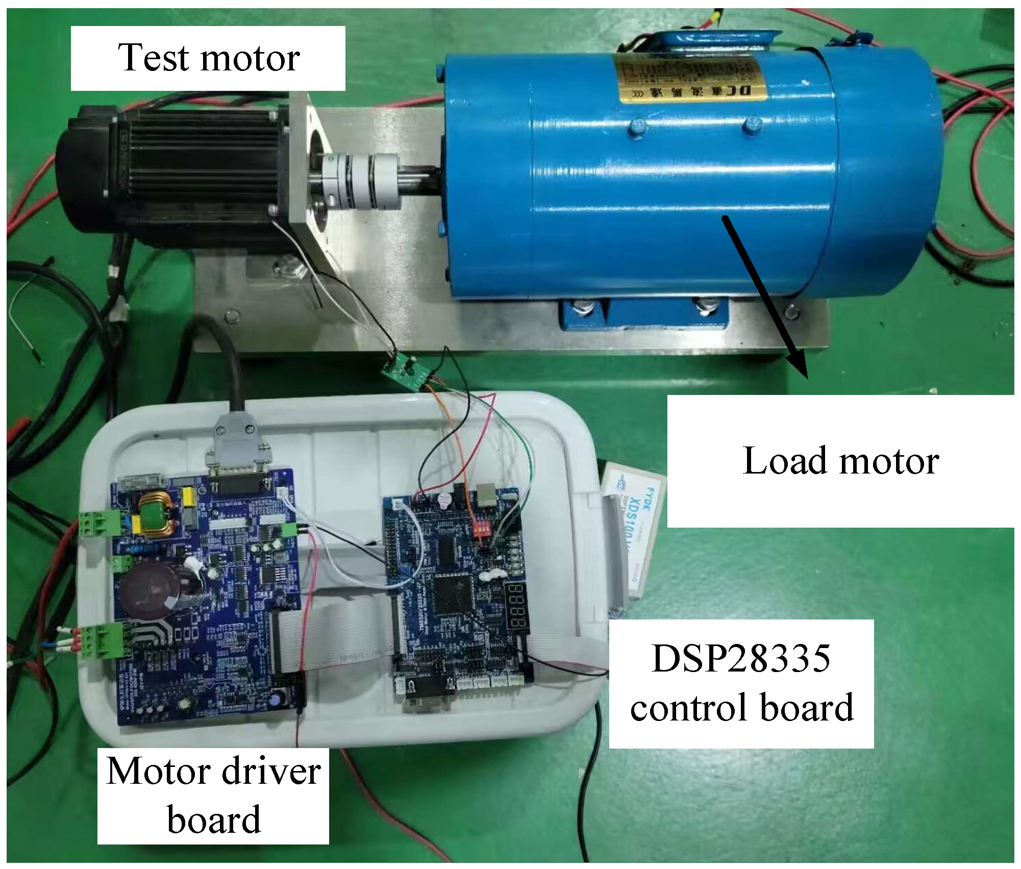
The experimental validation of the proposed control strategy was conducted using the constructed PMSM speed control system experimental platform. The experimental platform, based on the rotor flux-based sliding mode observer (SMO) and RBF-PID control strategy for PMSM systems, is shown in Figure 9.

The main parameters of the physical experimental platform are shown in

Table 2. Physical experimental platform parameters.

The Name of the Parameter	The Reference Value	Unit
Rated line voltage	220	V
Rated line current	3	A
Rated power	750	W
Rated speed	3000	r/min
Stator phase resistance	2.88	Ω
Inductance	6.4	mH
Permanent magnet flux linkage	0.049	Wb
Polar	4	/
Learning rate in RBF-NN	0.6	/

below:

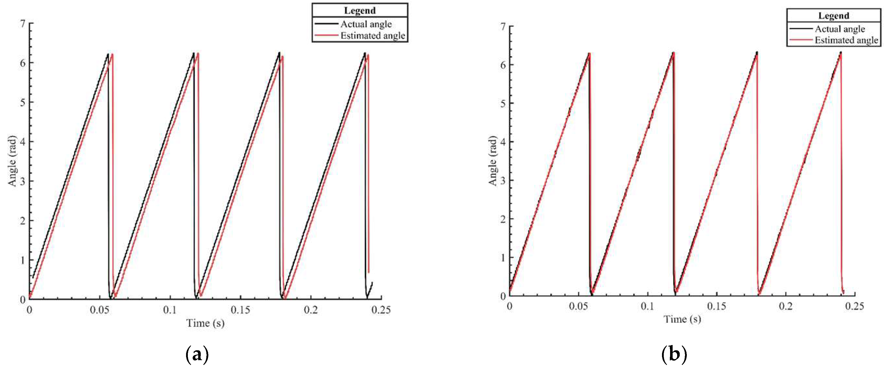
Figure 10a shows the electrical angle tracking curves of the traditional SMO observer and traditional PI controller at a motor speed of 1000 r/min. From the graph, it can be observed that the observed electrical angle by the traditional SMO significantly deviates from the angle measured by the encoder. There is a noticeable angular offset, indicating that the angle observation performance is not satisfactory.

Figure 10b displays the electrical angle tracking curves of the improved SMO observer and RBF-PID controller at a motor speed of 1000 r/min. From the graph, it can be seen that the observed electrical angle by the improved SMO exhibits a smaller deviation from the angle measured by the encoder. Compared to the traditional SMO, the angle observation effectiveness is greatly improved. The observed angle by the observer closely matches the actual angle measured by the encoder.

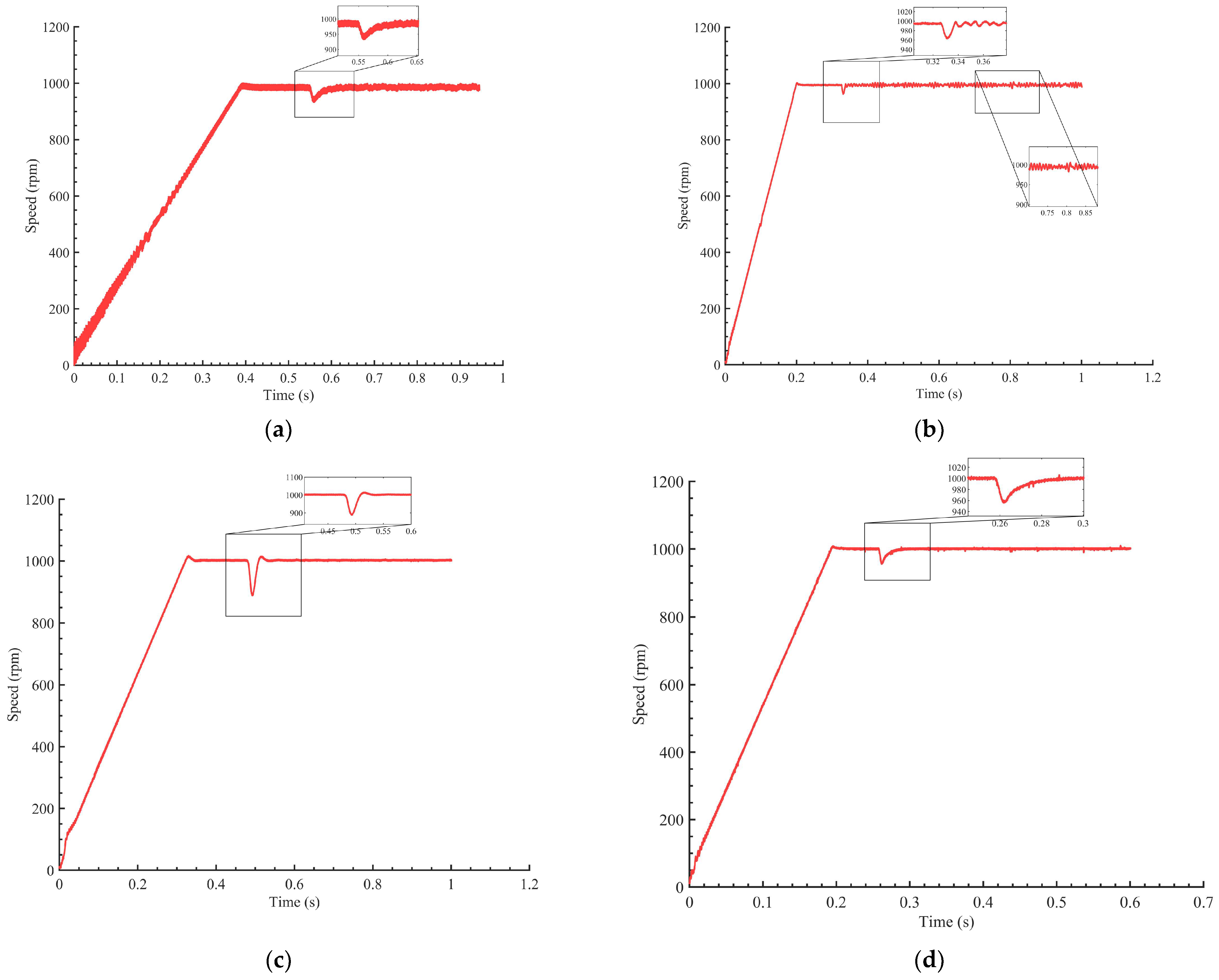
Figure 11a shows the speed curves of the traditional SMO observer and traditional PI controller during a load experiment at a motor speed of 1000 r/min. At 0.56 s, a torque load is applied. From the graph, it can be observed that the control performance of the estimated speed by the improved SMO is average, and there is an oscillation in the motor speed waveform after the load. Therefore, there is still room for improvement in the performance of the traditional SMO and PI control.

Figure 11b presents the curves of the traditional SMO observer and RBF-PID controller during a load experiment at a motor speed of 1000 r/min. From the graph, it can be observed that the conventional sliding mode observer combined with RBF-PID control reduces speed fluctuations, and a torque load is applied at 0.33 s. Compared to the traditional PI control, the speed fluctuations are effectively reduced.

Figure 11c presents the curves of the improved SMO observer and traditional controller during a load experiment at a motor speed of 1000 r/min. From the graph, it can be observed that when using the improved sliding mode observer algorithm, the speed fluctuations are significantly reduced compared to the traditional SMO. However, the traditional PI controller exhibits some overshoot in speed and load transients. At 0.45 s, a torque load is applied, and the motor speed exhibits a significant overshoot, indicating that there is room for improvement in the control effectiveness.

Figure 11d presents the curves of the improved SMO observer and RBF-PID controller during a load experiment at a motor speed of 1000 r/min. From the graph, it can be observed that the overall speed control performance of the motor is improved compared to the previous three methods. Moreover, even after adding a load, the motor speed quickly returns to its original speed with minimal fluctuations and reduced overshoot.

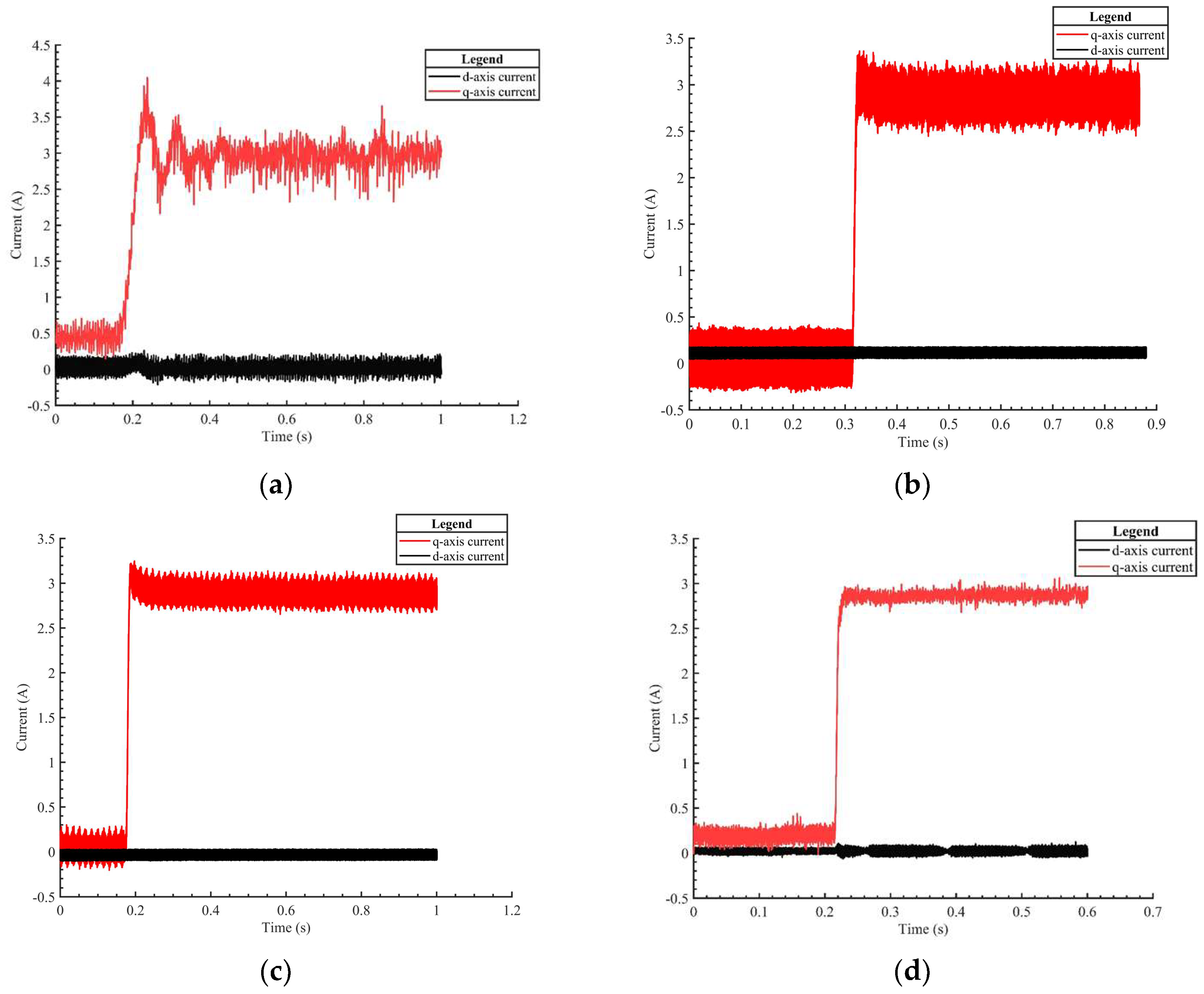
Figure 12a depicts the d-q axis current curves of the traditional SMO and traditional PI controllers during a load experiment at a motor speed of 1000 r/min. At 0.2 s, a torque load is applied. From the graph, it can be observed that both the traditional SMO and traditional PI controllers exhibit significant overshoot in the d-q axis current during the sudden load, and there is an oscillation in the motor current waveform after the load.

Figure 12b depicts the d-q axis current curves of the traditional SMO and RBF-PID controllers during a load experiment at a motor speed of 1000 r/min. At 0.45 s, a torque load is applied. From Figure 12b, it can be observed that compared to Figure 12a, under the control of RBF-PID, the overshoot of the q-axis current is reduced. However, there is still some current fluctuation that needs to be improved.

Figure 12c depicts the d-q axis current curves of the improved SMO and traditional PI controllers during a load experiment at a motor speed of 1000 r/min. At 0.19 s, a torque load is applied. From Figure 12c, it can be observed that compared to Figure 12a,b, under the improved SMO observer algorithm, the fluctuation of the q-axis current is reduced. However, there is still some overshoot in the q-axis current under the traditional PI control.

Figure 12d shows the d-q axis current curves of the improved SMO and RBF-PID controllers during a load experiment at a motor speed of 1000 r/min. From the graph, it can be observed that the improved SMO achieves better control of the estimated current, and at 0.21 s, a torque load is applied. It can be seen that the d-q axis current control is improved, with reduced overshoot and decreased current oscillation compared to the traditional SMO. This leads to a more accurate estimation of the electrical angle. Compared to the traditional SMO, the speed control performance is significantly enhanced.

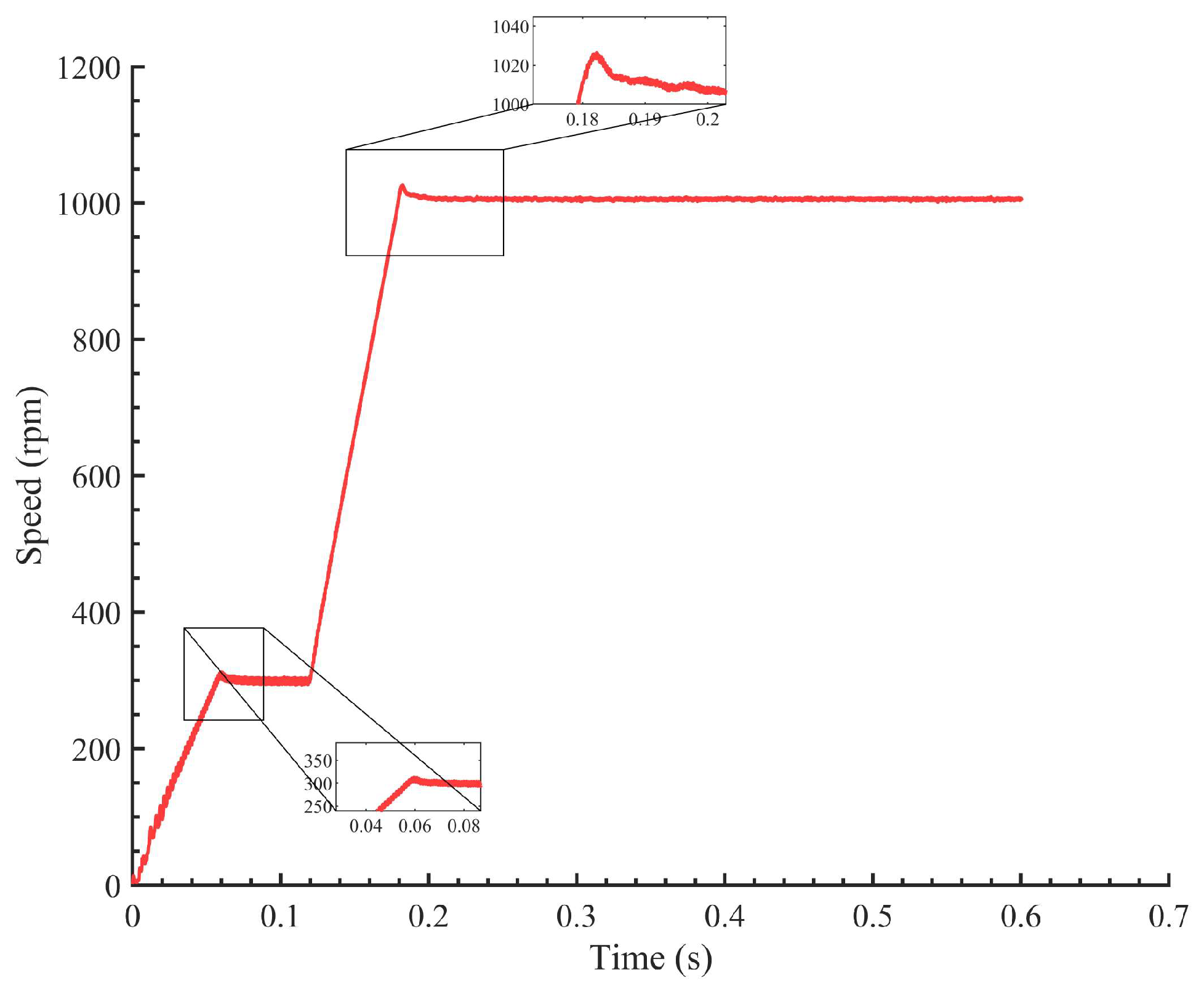
Figure 13 shows the experimental waveform of the motor speed with the improved SMO and RBF-PID during a sudden change in motor speed. The motor initially accelerates to 300 r/min; then, at 0.12 s, it undergoes a sudden acceleration to 1000 r/min. From the graph, it can be observed that the speed control achieves good performance with overshoot control within 25 r/min.

6. Conclusions

In this paper, we propose an improved rotor flux-based sliding mode observer (SMO) that utilizes the sigmoid function as a switching function, effectively reducing inherent chattering during sliding mode switching. We then combine the RBF-PID controller with the enhanced SMO to use neural networks for PI controller correction in the current loop, which can potentially identify other electrical parameters using gradient descent in the future. An RBF neural network is employed to identify the controlled object. Leveraging the Jacobian information of the controlled object identified by the RBF neural network, we dynamically adjust the gains of the current PI controller to achieve precise control of the d-q axis current.

Experimental results demonstrate that this control strategy exhibits good accuracy and disturbance rejection performance under different speeds and sudden load changes. Compared to traditional PI controllers, the RBF-PID controller outperforms in terms of motor overshoot, motor adjustment time, maximum synchronization error, and synchronization error adjustment time. Through these efforts, we support the improvement of the sliding mode observer’s accuracy in electrical angle estimation and motor control performance. This has significant implications in fields such as renewable energy, environmental protection, and industrial applications.