Abstract
In this study, a fault-tolerant control (FTC) tactic using a sliding mode controller–observer method for uncertain and faulty robotic manipulators is proposed. First, a finite-time disturbance observer (DO) is proposed based on the sliding mode observer to approximate the lumped uncertainties and faults (LUaF). The observer offers high precision, quick convergence, low chattering, and finite-time convergence estimating information. Then, the estimated signal is employed to construct an adaptive non-singular fast terminal sliding mode control law, in which an adaptive law is employed to approximate the switching gain. This estimation helps the controller automatically adapt to the LUaF. Consequently, the combination of the proposed controller–observer approach delivers better qualities such as increased position tracking accuracy, reducing chattering effect, providing finite-time convergence, and robustness against the effect of the LUaF. The Lyapunov theory is employed to illustrate the robotic system’s stability and finite-time convergence. Finally, simulations using a 2-DOF serial robotic manipulator verify the efficacy of the proposed method.
1. Introduction
In industry, robotic manipulators are very popular. They have been employed in many applications such as material handling, milling, painting welding, and roughing. The greater the importance of robotic manipulators in industry, the greater interest in the research field of control for robotic manipulators, which aims to make the robot tracks a desired trajectory with the greatest tracking accuracy [1,2]. However, in both theory and practice, robotic manipulators are difficult to control due to their characteristics. First, the dynamic of robotic manipulators is highly nonlinear and complicated, including the coupling effect. Furthermore, uncertainties in robot dynamics are also caused by payload fluctuations, frictions, external disturbances, etc. Therefore, it is arduous or even impossible to correctly identify the dynamics of robots. In some special cases, with the long-time operation, unknown faults might happen. The faults could be actuator faults, sensor faults, or process faults. They are big problems that have been challenged by many researchers. A variety of approaches for dealing with both the impact of uncertainties and faults have been presented in the current literature. The authors of [3,4,5] proposed methods to estimate the dynamics uncertainties and faults independently. However, using two distinct observers, on the other hand, makes the methods complex, requiring resources and time for calculation. In this study, faults are regarded as extra uncertainties, and the overall impacts of the system’s lumped uncertainties and faults (LUaF) are evaluated.
Fault-tolerant control (FTC) techniques have been developed to deal with the LUaF [6,7]. FTC techniques are broadly classified into two types: passive FTC (PFTC) [8,9] and active FTC (AFTC) [10,11,12]. A robust controller is built in the PFTC approach to manage the LUaF without the need for feedback input from a disturbance observer (DO). Because the effects of LUaF imposed on the typical controller of the PFTC are greater than those imposed on the notional controller of the AFTC, the nominal controller of the PFTC has the need of more resilience to eliminate the impacts of LUaF. By contrast, the AFTC is built using an online DO technology. As the LUaF is appropriately estimated, the AFTC provides better control effectiveness than the PFTC. As a result, the AFTC techniques are more suited for industrial cases.
In the literature, many efforts have been given for FTC problem of robotic manipulators, such as computed torque control [13,14], fuzzy logic control [15,16], adaptive control [17,18], neural network control [19,20], and sliding mode control (SMC) [21,22,23]. Among them, the SMC is one of the most powerful robust controllers which can be used in uncertainty nonlinear dynamic systems. In recent years, the SMC has been developed in a wide range of area by many researchers due to its simple design procedure while providing acceptable control performance. It also has the ability to solve the two main crucial challenging issues in control that are stability and robustness [24,25]. Although providing wonderful control properties, some problems that reduce the applicability of the conventional SMC still exist. These include the inability to ensure finite-time convergence and the chattering phenomena, which is the high-frequency oscillation of the control input signal.
To guarantee the finite-time convergence of the tracking error, many efforts have been made. In [26,27,28], the terminal SMC (TSMC) has been developed. As compared to the traditional SMC, the TSMC has better precision and overcomes the finite-time convergence problem; however, as a trade-off, its convergence time is slightly slower. In addition, the singularity problems are appeared in some special cases. To resolve the two disadvantages, the fast TSMC (FTSMC) [29,30,31] and the non-singular TSMC (NTSMC) [32,33] are used. Unfortunately, the two controllers just solve the two problems separately. In order to get rid of them simultaneously, the non-singular fast TSMC (NFTSMC) is proposed [34,35,36,37,38]. This controller has outstanding control features such as singularity removal, high tracking precision, finite-time convergence, and durability to LUaF effects.
To decrease chattering caused by the adoption of a discontinuous reaching control rule with a large and fixed gain, the fundamental concept is to employ an observer to approximate the LUaF and then compensate for its impacts on the system. Using this technique, a smaller switching gain can be set to deal with the impacts of the estimated error rather than the effects of the LUaF. Therefore, the chattering phenomenon could be reduced. In the present literature, many researchers have been focusing their efforts on building an effective observer to estimate the LUaF [39,40,41,42,43,44,45], for example, neural network (NN) observer [41,42], extended state observer (ESO) [43], and second-order sliding mode observer (SOSMO) [44,45]. The NN observer has been frequently used due to its learning capacity and high accuracy estimation. Nevertheless, the learning capability complicates the system and necessitates a higher system configuration in order to employ online training approaches, which raises the cost of equipment. The ESO is a simple technique for online observation, which provides quite good approximation information. Thanks to the linear characteristic of the observer element, which can strongly deal with perturbations that are very far away from the origin, the convergence speed of the ESO is very high. However, the overshoot phenomenon at the convergence stage reduces its application ability. By contrast, the SOSMO has the ability to estimate the LUaF without the overshoot phenomenon as in ESO, however, the convergence time is a little slower. In addition, a lowpass filter is needed to reconstruct the estimated LUaF, which reduces its estimation accuracy.
From the motivation above, this study proposed a disturbance observer (DO) to approximate the LUaF of robotic manipulator system with high accuracy and fast convergence. To attain high positional tracking accuracy and system stability under the impacts of the LUaF, an FTC technique combining the adaptive NFTSMC and the suggested DO, named A-NFTSMC-DO, is proposed. In the controller, an adaptive law is applied to estimate the switching gain to help the controller automatically adapts with the LUaF. Therefore, the combination of proposed controller–observer technique provides high tracking precision, fast convergence, less chattering effect, and finite-time convergence. The following are the main contributions of this research:
- (1)
- Proposing a DO to approximate the LUaF with high accuracy and fast convergence.
- (2)
- Proposing an FTC technique for improving the tracking performance of the robot manipulator while taking to account the overall impacts of the LUaF.
- (3)
- Minimizing the phenomena of chattering in control input signals.
- (4)
- Using the Lyapunov stability theory to demonstrate the system’s finite-time stability.
The following is the structure of the research. Section 2 follows the introduction by presenting the dynamic equation of a serial robotic manipulator. Section 3 then depicts the suggested architecture of the DO. In Section 4, the A-NFTSMC-DO is designed to obtain a minimal tracking error. In Section 5, the simulations of the proposed algorithm are executed on a 2-DOF serial robotic manipulator. Finally, Section 6 gives some conclusions.
2. System Modeling and Problem Formulation
The following is a description of a serial robotic manipulator with a dynamic equation in Lagrangian form:
where are the vectors that represent robot joint angular positions, velocities, and accelerations, respectively; is the matrix of inertia, which is symmetric, bounded, and positive definite; is the matrix of the Coriolis and centripetal forces; is the vector of the control input torques; and , , and are the vector of the gravitational forces, friction, and disturbance, respectively.
Equation (1) can be transformed to the form below:
where and represent the uncertainty terms.
Faults in a system have been growing much more common in current industrial applications as they get more sophisticated, particularly under the state of enduring implementation. As a result, this article supposes that the robot system operates under the impact of faults. In these cases, the robot dynamic Equation (2) can be rewritten as
where represents the unknown faults. is occurrence time and the term denotes the time profile of faults with , denotes the evolution rate of faults.
Remark 1.
In robotic manipulator systems, the unknown faults can be actuator faults, sensor faults, and process faults. In this paper, the effects of actuator faults in the system are considered. Therefore, the fault functions are defined as faults that occur at the actuator.
Basically, the robotic system (3) is reconstructed in state space as
where , , and denotes the LUaF.
The main purpose of this study is to design an FTC scheme for the robotic manipulator such that the robot can track the desired trajectory under the effect of the LUaF with minimal tracking error. The FTC scheme is constructed according to the assumptions as follows.
Assumption 1.
The desired trajectory is bounded and is a twice continuously differentiable function respect to time.
Assumption 2.
The LUaF is bounded as
where is a positive constant.
3. Estimation Scheme
3.1. Design of Disturbance Observer
The DO is developed to be used with the robot manipulator system (4) as
where is the estimator of the true state , and represent the observer gains.
By subtracting (6) from (4), we can obtain
where represents the state estimation errors.
Equation (7) can be rewritten as
Theorem 1.
For the robotic system given in (4), if the DO is designed as (6) with suitable chosen observer gains, then the system is stable and the estimation error in (8) will converge to zero in finite-time.
Proof of Theorem 1.
(see Appendix A). □
3.2. The LUaF Reconstruction
After the convergence time, the predicted states, , will approach the real states after the convergence time, ; thus, the estimation error (7) becomes
Therefore, the estimation of the LUaF can be reconstructed as
Remark 2.
Thanks to the characteristic of linear terms, the proposed DO can obtain higher convergence speed compared to the SOSMO. This excellent property will be confirmed in the simulation part.
Remark 3.
As shown in (10), the resulting signal is made up of an integral operator; thus, the estimated information of the suggested DO may be rebuilt directly without filtration. As a result, this observer produces a more accurate estimation signal with less chattering than the SOSMO. In the following part, this estimation information will be used to build the FTC technique.
4. Design of Controller
4.1. The DO-Based NFTSMC
We define the position tracking and velocity errors as
where are the desired trajectories and velocities, respectively.
An NFTSM function is chosen as in [46]:
where constants are positive constants and can be selected as
The control law is designed as follows:
The switching control law, , is employed to compensate for the estimation errors as follows:
where is a small positive constant and denotes the switching gain, which is bounded as with represents the estimation error.
Theorem 2.
For the uncertain and faulty robotic manipulator described in (4), if the proposed control law is designed as in (14)–(17) and the NFTSM function is selected as in (12), then the stability and finite-time convergence of the system are guaranteed.
Proof of Theorem 2.
(see Appendix B). □
Remark 4.
The switching gain,
, is dependent on the accuracy of the observer. In the next section, an adaptive NFTSMC will be proposed to help the controller automatically adapts with the LUaF.
4.2. The DO-Based Adaptive NFTSMC
An adaptive NFTSMC law is suggested as
where is the estimator of the ideal switching gain, , and is updated by the following adaptive law:
where is the adaptation gain.
Theorem 3.
For the uncertain and faulty robotic manipulator described in (4), if the proposed DO-based adaptive NFTSMC law is designed as in (18)–(21) and the NFTSM function is selected as in (12), then the stability and finite-time convergence of the system are guaranteed.
Proof of Theorem 3.
(see Appendix C). □
Remark 5.
Generally, the sliding motion only can archive in ideal condition, thus, the switching gain in (22) keeps increasing continuously. This problem is well known as the “parameter drift problem”. To solve this problem, the following adaptive law can be utilized:
where is a sufficiently small constant.
The structure of the proposed FTC strategy is described in Figure 1.
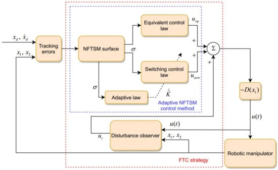
Figure 1.
Structure of the proposed FTC strategy.
5. Numerical Simulations
Computer simulations on a 2-DOF robotic manipulator are used to show the utility of the suggested controller-observer approach. The 2-DOF model is illustrated in Figure 2, and its dynamic model is described below.
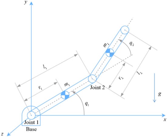
Figure 2.
Configuration of the 2-DOF robotic manipulator.
Inertia term:
where
Coriolis and centripetal term:
Gravitational term:
The parameters of the 2-DOF robot are given as in Table 1.

Table 1.
Parameters of the 2-link robot manipulator.
All simulations in this work are carried out using MATLAB/Simulink and the sampling time is s.
The desired trajectories of robot are assumed as
The friction and disturbance are, respectively, assumed as
The fault is assumed to occur to joint 1 at s and occur to joint 2 at s
The simulation is divided into two parts. First, a comparison of the proposed DO, the SOSMO [44], the ESO [43], and the DO in [47] is performed. Second, the tracking performance of the proposed A-NFTSMC-DO will be compared with the conventional SMC and the NFTSMC to show its superior control properties.
The parameters of the observer and controller are shown in the Table 2.
Table 2.
The values of the controller/observer’s parameters.
For the first part, the result of the comparison is presented in Figure 3 and Figure 4. Figure 3 shows the estimation results of LUaF estimation among four observers. Figure 4 shows the estimation error at each joint. As shown in the result, the ESO (the blue solid line) provides fast estimation result, however, the overshoot phenomenon at the convergence stage is the main disadvantage of the ESO. By contrast, the SOSMO (the green solid line) provides estimation result without the overshoot phenomenon as in ESO, however, the convergence time is a little slower. In addition, a low-pass filter is needed to reconstruct the estimated LUaF. In terms of estimation accuracy, both the ESO and SOSMO provide quite good estimation result in normal operation condition; however, when faults occur, the estimation errors become larger. The proposed DO (the red solid line) provides the LUaF estimation with a faster convergence speed compared to the SOSMO due to the linear characteristic of the observer elements. Compared to the ESO, the proposed DO eliminates the overshoot phenomenon. In addition, it achieves the highest estimation accuracy among three observers in both before and after faults occur. Moreover, the LUaF can be reconstructed directly without the need of a low-pass filter. Compared to the DO in [47], the proposed DO obtains almost the same estimation accuracy, however, the estimation speed is faster.
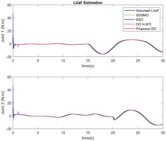
Figure 3.
The estimation of LUaF among four observers.
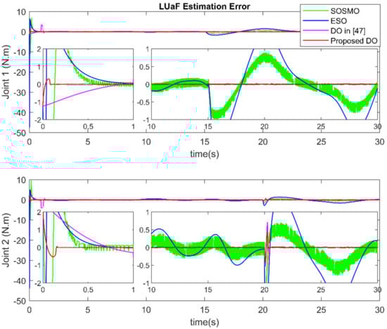
Figure 4.
The LUaF estimation error at each joint.
In the second part, in order to show the effectiveness of the proposed A-NFTSMC-DO method, its control performance will be compared with the two controllers: the conventional SMC and the NFTSMC. The results are shown in Figure 5, Figure 6 and Figure 7. Figure 5 and Figure 6 show the robot end-effector tracking and the joint tracking error among three controllers. As in the results, the SMC provides acceptable tracking performance. However, compared to others, its tracking error (the blue solid line) has the lowest accuracy. In addition, in terms of convergence speed, the conventional SMC takes a longer time for convergence. On the other hand, the NFTSMC (the green solid line) offers both higher tracking accuracy and faster convergence compared to the SMC. The proposed FTC method (the red solid line) offers the tracking error with the same convergence speed as the NFTSMC, meanwhile, it provides the highest tracking accuracy compared to others. Figure 7 shows the comparison of control input torque. As a result of the LUaF compensation, the switching gain parameter of the control law is now extremely small. Therefore, as we can see, the suggested A-NFTSMC-DO delivers reduced chattering control input torque. Furthermore, because of better characteristics of the adaptive law, the suggested controller can automatically adjust with the LUaF. The estimated value of the sliding gain is shown in Figure 8.
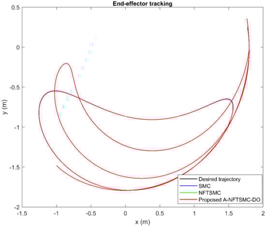
Figure 5.
Robot end-effector tracking.
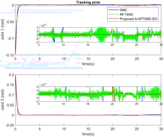
Figure 6.
Tracking error at each joint.
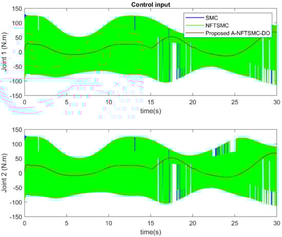
Figure 7.
Control input at each joint.
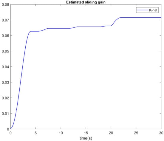
Figure 8.
Estimation of sliding gain.
6. Conclusions
In this study, an FTC strategy using an A-NFTSMC based on a DO for uncertain and faulty robotic manipulators is proposed. The suggested observer demonstrated its capacity to estimate the LUaF with excellent accuracy, rapid convergence, and almost no chattering. They will then be used to compensate for the impacts on the system, which improves the tracking performance of the suggested FTC technique. The suggested FTC technique has advanced control characteristics of high positioning tracking accuracy with quick finite-time convergence, chattering phenomena minimization, and LUaF robustness. The use of Lyapunov theory ensures system stability and finite-time convergence. The efficacy of the suggested method has been confirmed by computer simulation on a 2-DOF robot.
Author Contributions
Conceptualization, V.-C.N. and P.-N.L.; methodology, V.-C.N. and P.-N.L.; software, V.-C.N. and H.-J.K.; validation, P.-N.L.; formal analysis, V.-C.N. and H.-J.K.; investigation, H.-J.K.; resources, P.-N.L. and H.-J.K.; data curation, V.-C.N. and P.-N.L.; writing—original draft preparation, V.-C.N. and P.-N.L.; writing—review and editing, V.-C.N., P.-N.L. and H.-J.K.; visualization, P.-N.L.; supervision, H.-J.K.; project administration, H.-J.K.; funding acquisition, H.-J.K. All authors have read and agreed to the published version of the manuscript.
Funding
This research was supported by Basic Science Research Program through the National Research Foundation of Korea (NRF) funded by the Ministry of Education (2019R1D1A3A03103528).
Institutional Review Board Statement
Not applicable.
Informed Consent Statement
Not applicable.
Data Availability Statement
Not applicable.
Conflicts of Interest
The authors declare no conflict of interest.
Appendix A
Proof of Theorem 1.
A suitable Lyapunov function is selected as
The Lyapunov function (A1) can be written as a quadratic form where
, and .
The time derivative of the Lyapunov function is calculated as
where
Using the similar process as in the proof of Theorem 5 in [45], it can be concluded that the system is stable, and the estimation error in (8) will approach to zero in finite-time. Accordingly, Theorem 1 is clearly illustrated. □
Appendix B
Proof of Theorem 2.
Taking the derivative of the sliding function (12) with respect to time, we obtain
Inserting the control laws (14)–(17) into (A3) yields
A candidate Lyapunov function is chosen as
Taking the derivative of the Lyapunov function (A5) and substituting the result from (A4), we obtain
Therefore, the Theorem 2 is successfully proven. □
Appendix C
Proof of Theorem 3.
The candidate Lyapunov function is chosen as
where .
Using the similar process as in the proof of Theorem 2, the Theorem 3 is successfully proven. □
References
- Chen, D.; Zhang, Y.; Li, S. Tracking control of robot manipulators with unknown models: A jacobian-matrix-adaption method. IEEE Trans. Ind. Inform. 2017, 14, 3044–3053. [Google Scholar] [CrossRef]
- Jin, L.; Li, S.; Yu, J.; He, J. Robot manipulator control using neural networks: A survey. Neurocomputing 2018, 285, 23–34. [Google Scholar] [CrossRef]
- Hamedani, M.H.; Zekri, M.; Sheikholeslam, F.; Salvaggio, M.; Ficuciello, F.; Siciliano, B. Recurrent Fuzzy Wavelet Neural Network Variable Impedance Control of Robotic Manipulators with Fuzzy Gain Dynamic Surface in an Unknown Varied Environment. Fuzzy Sets Syst. 2021, 416, 1–26. [Google Scholar] [CrossRef]
- Huang, S.N.; Tan, K.K.; Lee, T.H. Automated fault detection and diagnosis in mechanical systems. IEEE Trans. Syst. Man Cybern. Part C Appl. Rev. 2007, 37, 1360–1364. [Google Scholar] [CrossRef]
- Van, M.; Kang, H.-J.; Suh, Y.-S.; Shin, K.-S. A Robust Fault Diagnosis and Accommodation Scheme for Robot Manipulators. Int. J. Control Autom. Syst. 2013, 11, 377–388. [Google Scholar] [CrossRef]
- Zhang, Y.; Jiang, J. Bibliographical review on reconfigurable fault-tolerant control systems. Annu. Rev. Control 2008, 32, 229–252. [Google Scholar] [CrossRef]
- Zhang, C.; Dai, M.-Z.; Dong, P.; Leung, H.; Wang, J. Fault-Tolerant Attitude Stabilization for Spacecraft with Low-Frequency Actuator Updates: An Integral-Type Event-Triggered Approach. IEEE Trans. Aerosp. Electron. Syst. 2020, 57, 729–737. [Google Scholar] [CrossRef]
- Benosman, M.; Lum, K.-Y. Passive actuators’ fault-tolerant control for affine nonlinear systems. IEEE Trans. Control Syst. Technol. 2009, 18, 152–163. [Google Scholar] [CrossRef]
- Stefanovski, J.D. Passive fault tolerant perfect tracking with additive faults. Automatica 2018, 87, 432–436. [Google Scholar] [CrossRef]
- Sadeghzadeh, I.; Mehta, A.; Chamseddine, A.; Zhang, Y. Active Fault Tolerant Control of a Quadrotor Uav Based on Gainscheduled Pid Control. In Proceedings of the 2012 25th IEEE Canadian Conference on Electrical and Computer Engineering (CCECE), Montreal, QC, Canada, 29 April–2 May 2012; pp. 1–4. [Google Scholar]
- Shen, Q.; Yue, C.; Goh, C.H.; Wang, D. Active fault-tolerant control system design for spacecraft attitude maneuvers with actuator saturation and faults. IEEE Trans. Ind. Electron. 2018, 66, 3763–3772. [Google Scholar] [CrossRef]
- Vo, A.T.; Kang, H.-J. A novel fault-tolerant control method for robot manipulators based on non-singular fast terminal sliding mode control and disturbance observer. IEEE Access 2020, 8, 109388–109400. [Google Scholar] [CrossRef]
- Zhao, B.; Li, Y. Local joint information based active fault tolerant control for reconfigurable manipulator. Nonlinear Dyn. 2014, 77, 859–876. [Google Scholar] [CrossRef]
- Codourey, A. Dynamic modeling of parallel robots for computed-torque control implementation. Int. J. Robot. Res. 1998, 17, 1325–1336. [Google Scholar] [CrossRef]
- Yang, C.; Jiang, Y.; Na, J.; Li, Z.; Cheng, L.; Su, C.-Y. Finite-time convergence adaptive fuzzy control for dual-arm robot with unknown kinematics and dynamics. IEEE Trans. Fuzzy Syst. 2018, 27, 574–588. [Google Scholar] [CrossRef]
- Ling, S.; Wang, H.; Liu, P.X. Adaptive fuzzy dynamic surface control of flexible-joint robot systems with input saturation. IEEE/CAA J. Autom. Sin. 2019, 6, 97–106. [Google Scholar] [CrossRef]
- Li, M.; Li, Y.; Ge, S.S.; Lee, T.H. Adaptive control of robotic manipulators with unified motion constraints. IEEE Trans. Syst. Man Cybern. Syst. 2016, 47, 184–194. [Google Scholar] [CrossRef] [Green Version]
- Wu, Y.; Huang, R.; Li, X.; Liu, S. Adaptive neural network control of uncertain robotic manipulators with external disturbance and time-varying output constraints. Neurocomputing 2019, 323, 108–116. [Google Scholar] [CrossRef]
- Luan, F.; Na, J.; Huang, Y.; Gao, G. Adaptive neural network control for robotic manipulators with guaranteed finite-time convergence. Neurocomputing 2019, 337, 153–164. [Google Scholar] [CrossRef]
- Wang, L.; Chai, T.; Zhai, L. Neural-network-based terminal sliding-mode control of robotic manipulators including actuator dynamics. IEEE Trans. Ind. Electron. 2009, 56, 3296–3304. [Google Scholar] [CrossRef]
- Ha, Q.P.; Rye, D.C.; Durrant-Whyte, H.F. Fuzzy moving sliding mode control with application to robotic manipulators. Automatica 1999, 35, 607–616. [Google Scholar] [CrossRef]
- Yu, S.; Yu, X.; Shirinzadeh, B.; Man, Z. Continuous finite-time control for robotic manipulators with terminal sliding mode. Automatica 2005, 41, 1957–1964. [Google Scholar] [CrossRef]
- He, S.; Song, J. Finite-time sliding mode control design for a class of uncertain conic nonlinear systems. IEEE/CAA J. Autom. Sin. 2017, 4, 809–816. [Google Scholar] [CrossRef]
- Utkin, V.I. Sliding Modes in Control and Optimization; Springer Science & Business Media: Berlin/Heidelberg, Germany, 2013. [Google Scholar]
- Nguyen, V.-C.; Vo, A.-T.; Kang, H.-J. Continuous PID Sliding Mode Control Based on Neural Third Order Sliding Mode Observer for Robotic Manipulators. In Proceedings of the International Conference on Intelligent Computing, Sardinia, Italy, 3–5 June 2019; pp. 167–178. [Google Scholar]
- Zhihong, M.; Paplinski, A.P.; Wu, H.R. A robust MIMO terminal sliding mode control scheme for rigid robotic manipulators. IEEE Trans. Automat. Control 1994, 39, 2464–2469. [Google Scholar] [CrossRef]
- Wang, H.; Man, Z.; Kong, H.; Zhao, Y.; Yu, M.; Cao, Z.; Zheng, J.; Do, M.T. Design and implementation of adaptive terminal sliding-mode control on a steer-by-wire equipped road vehicle. IEEE Trans. Ind. Electron. 2016, 63, 5774–5785. [Google Scholar] [CrossRef]
- Nguyen, V.-C.; Le, P.-N.; Kang, H.-J. Model-Free Continuous Fuzzy Terminal Sliding Mode Control for Second-Order Nonlinear Systems. In Proceedings of the International Conference on Intelligent Computing, New York, NY, USA, 21–25 June 2021; pp. 245–258. [Google Scholar]
- Madani, T.; Daachi, B.; Djouani, K. Modular-controller-design-based fast terminal sliding mode for articulated exoskeleton systems. IEEE Trans. Control Syst. Technol. 2016, 25, 1133–1140. [Google Scholar] [CrossRef]
- Solis, C.U.; Clempner, J.B.; Poznyak, A.S. Fast terminal sliding-mode control with an integral filter applied to a Van Der Pol oscillator. IEEE Trans. Ind. Electron. 2017, 64, 5622–5628. [Google Scholar] [CrossRef]
- Truong, T.N.; Vo, A.T.; Kang, H.-J. Implementation of an Adaptive Neural Terminal Sliding Mode for Tracking Control of Magnetic Levitation Systems. IEEE Access 2020, 8, 206931–206941. [Google Scholar] [CrossRef]
- Eshghi, S.; Varatharajoo, R. Nonsingular terminal sliding mode control technique for attitude tracking problem of a small satellite with combined energy and attitude control system (CEACS). Aerosp. Sci. Technol. 2018, 76, 14–26. [Google Scholar] [CrossRef]
- Lin, C.-K. Nonsingular terminal sliding mode control of robot manipulators using fuzzy wavelet networks. IEEE Trans. Fuzzy Syst. 2006, 14, 849–859. [Google Scholar] [CrossRef]
- Van, M.; Mavrovouniotis, M.; Ge, S.S. An adaptive backstepping nonsingular fast terminal sliding mode control for robust fault tolerant control of robot manipulators. IEEE Trans. Syst. Man Cybern. Syst. 2018, 49, 1448–1458. [Google Scholar] [CrossRef] [Green Version]
- Nguyen, V.-C.; Vo, A.-T.; Kang, H.-J. A Non-singular Fast Terminal Sliding Mode Control Based on Third-Order Sliding Mode Observer for a Class of Second-Order Uncertain Nonlinear Systems and Its Application to Robot Manipulators. IEEE Access 2020, 8, 78109–78120. [Google Scholar] [CrossRef]
- Anh Tuan, V.; Kang, H.-J. A new finite time control solution for robotic manipulators based on nonsingular fast terminal sliding variables and the adaptive super-twisting scheme. J. Comput. Nonlinear Dyn. 2019, 14, 031002. [Google Scholar] [CrossRef]
- Nguyen, V.-C.; Vo, A.-T.; Kang, H.-J. A Finite-Time Fault-Tolerant Control Using Non-Singular Fast Terminal Sliding Mode Control and Third-Order Sliding Mode Observer for Robotic Manipulators. IEEE Access 2021, 9, 31225–31235. [Google Scholar] [CrossRef]
- Nguyen, V.-C.; Kang, H.-J. A Fault Tolerant Control for Robotic Manipulators Using Adaptive Non-singular Fast Terminal Sliding Mode Control Based on Neural Third Order Sliding Mode Observer. In Proceedings of the International Conference on Intelligent Computing, Sanya, China, 4–6 December 2020; pp. 202–212. [Google Scholar]
- Zhou, M.; Cao, Z.; Zhou, M.; Wang, J.; Wang, Z. Zonotoptic fault estimation for discrete-time LPV systems with bounded parametric uncertainty. IEEE Trans. Intell. Transp. Syst. 2019, 21, 690–700. [Google Scholar] [CrossRef]
- Kazemi, H.; Yazdizadeh, A. Optimal state estimation and fault diagnosis for a class of nonlinear systems. IEEE/CAA J. Autom. Sin. 2017, 1–10. [Google Scholar] [CrossRef]
- Salgado, I.; Chairez, I. Adaptive unknown input estimation by sliding modes and differential neural network observer. IEEE Trans. Neural Netw. Learn. Syst. 2018, 29, 3499–3509. [Google Scholar] [CrossRef]
- Abdollahi, F.; Talebi, H.A.; Patel, R.V. A Stable Neural Network Observer with Application to Flexible-Joint Manipulators. In Proceedings of the 9th International Conference on Neural Information Processing, 2002, ICONIP ’02, Singapore, 18–22 November 2002; IEEE: Piscataway, NJ, USA, 2002; Volume 4, pp. 1910–1914. [Google Scholar] [CrossRef]
- Le, Q.D.; Kang, H.-J. Implementation of Fault-Tolerant Control for a Robot Manipulator Based on Synchronous Sliding Mode Control. Appl. Sci. 2020, 10, 2534. [Google Scholar] [CrossRef] [Green Version]
- Davila, J.; Fridman, L.; Levant, A. Second-order sliding-mode observer for mechanical systems. IEEE Trans. Automat. Control 2005, 50, 1785–1789. [Google Scholar] [CrossRef]
- Moreno, J.A.; Osorio, M. A Lyapunov Approach to Second-Order Sliding Mode Controllers and Observers. In Proceedings of the 2008 47th IEEE Conference on Decision and Control, Cancun, Mexico, 9–11 December 2008; pp. 2856–2861. [Google Scholar]
- Tran, X.-T.; Kang, H.-J. A Novel Adaptive Finite-Time Control Method for a Class of Uncertain Nonlinear Systems. Int. J. Precis. Eng. Manuf. 2015, 16, 2647–2654. [Google Scholar] [CrossRef]
- Gao, Z.; Guo, G. Fixed-time sliding mode formation control of AUVs based on a disturbance observer. IEEE/CAA J. Autom. Sin. 2020, 7, 539–545. [Google Scholar] [CrossRef]
Publisher’s Note: MDPI stays neutral with regard to jurisdictional claims in published maps and institutional affiliations. |
© 2021 by the authors. Licensee MDPI, Basel, Switzerland. This article is an open access article distributed under the terms and conditions of the Creative Commons Attribution (CC BY) license (https://creativecommons.org/licenses/by/4.0/).