Path Planning for Automatic Guided Vehicles (AGVs) Fusing MH-RRT with Improved TEB

Abstract

In this paper, an AGV path planning method fusing multiple heuristics rapidly exploring random tree (MH-RRT) with an improved two-step Timed Elastic Band (TEB) is proposed. The modified RRT integrating multiple heuristics can search a safer, optimal and faster converge global path within a short time, and the improved TEB can optimize both path smoothness and path length. The method is composed of a global path planning procedure and a local path planning procedure, and the Receding Horizon Planning (RHP) strategy is adopted to fuse these two modules. Firstly, the MH-RRT is utilized to generate a state tree structure as prior knowledge, as well as the global path. Then, a receding horizon window is established to select the local goal point. On this basis, an improved two-step TEB is designed to optimize the local path if the current global path is feasible. Various simulations both on static and dynamic environments are conducted to clarify the performance of the proposed MH-RRT and the improved two-step TEB. Furthermore, real applicative experiments verified the effectiveness of the proposed approach.

1. Introduction

With the merits of high automation and safe and reliable operation, automatic guided vehicles (AGVs) play a significant role in various fields [1], especially in transportation, the logistics industry [2] and autonomous driving [3]. AGV is an intelligent system integrating environment perception, planning, decision and control, and belongs to the category of wheeled mobile robot [4]. As a fundamental research topic in robotics, path planning has been received considerable attention. Generally speaking, the global path planning problem can be defined by determining a collision-free trajectory between the robot’s start position and its destination. In addition, local trajectory optimization is also important because of the time optimal and energy optimal requirement. In closed environments such as factories, fixed guided lines are adopted in order to improve reliability [5]. However, open scenarios need a safer and more real-time path planning method, so as to deal with uncertain obstacles. To achieve full autonomy in increasingly complex and highly dynamic environments, the efficiency and robustness of the trajectory generation are essential.

Due to its comprehensive applications, many researchers focus on the study of different path planning algorithms. The artificial potential field algorithms (ARFs) find the feasible trajectory by following the direction of the steepest descent of the potential [6,7]. However, they often end up in a local minimum. The graph searching algorithms, such as the Dijkstra [8] and A* [9], can always find the optimal trajectory if it exists. However, the time cost and memory usage increase exponentially as the problem scale increases. Sampling-based algorithms, such as the probabilistic roadmap algorithm (PRM) [10] and rapidly exploring random tree (RRT) [11], have been proven effective in solving many tough planning problems, particularly with real-time nonlinear systems. The sampling-based path planners incrementally construct the set of paths by iteratively adding random samples. It is noted that the sampling-based algorithms provide a probabilistic completeness. As the number of iterations goes to infinity, the probability of finding a solution path approaches 1 if it exits. Both sampling-based and graph search algorithms can be used to perform as global planners. Limited by global prior map, the latter are usually used in static environment.

In a dynamic environment, the planned trajectory may become invalid. The path should be optimized to respond to the dynamic environment in real time for AG. Incremental search algorithms are preferable over the traditional methods in dynamic environments due to serveral additional candidate paths. The tree structure of the RRT makes it useful for incremental path planning [12]. However, the tree structure of the original RRT focuses on the speed in finding planning solutions and generating trajectories, with less regard to the solution optimality and stability [13]. Following the original RRT, many variants of the RRT algorithms appeared inspired concerning heuristic elements. RRT-connect works by incrementally building two RRTs rooted at the start and the goal configurations [14]. The trees each explore space around them and also advance towards each other through the use of a simple greedy heuristic. Apart from the above-mentioned types of methods, EB-RRT combine time-based RRT with elastic band (EB), and achieve the optimal heuristic trajectory in the homology class of the heuristic trajectory [15]. While the above methods reduced the path-searching time, Karaman et al. [16] proved that the RRT converges surely to non-optimal values and developed an asymptotically optimal RRT-based path planning scheme called optimal rapidly exploring random tree (RRT*), which makes use of a new step to rewire the neighboring vertices of the newly inserted node. The dual tree RRT* (DT-RRT*) separates the extension and optimization procedure using a double-tree structure [17]. One is original RRT, another is modified RRT*. In addition, Wang et al. [18] proposed KB-RRT* algorithm, which added kinematic constraints and used branch pruning for further optimization. As a significant extension of the RRT*, Informed RRT* establishes oval shaped sampling space to reduce the path length of the RRT* [19].

In contrast to sample-based methods, a richer space of trajectory options are output by the optimization. The initial trajectories generated by RRTs mostly need to be optimized, not only concerning path length but also path smoothness. Therefore, the Bezier curve is incorporated in RRT algorithms to achieve path smoothing, where a novel local path planner is proposed to generate a smooth path. Besides, the timed elastic band (TEB), first introduced in [20], one of the value-optimal based methods, can be used to quickly adjust the current trajectory and is good at local optimization. Its principle is similar to rubber band deformation, connecting the starting point and the target point, solving by imposing a series of constraints and designing the objective function, which is essentially a multi-objective function optimization problem. As a result, TEB is suitable for incorporating with RRT to jointly plan the optimal path.

Considering transport logistics applications and constraints of AGVs, optimal criteria could be based on one or more conditions such as shortest physical distance, smoothness, low risk, less fuel requirements, maximum area coverage, and low energy consumption. So far, few works consider both dynamics and kinematics, and most of them prefer improving convergence speed while ignoring the path optimality. For differential wheeled AGVs in traffic and logistics industry, planning path should satisfy at least three basic requirements, high safety, stability, and real-time. Hence, in the perspective of path planning for differential wheeled AGVs optimal path refers to finding a feasible and smooth solution with optimized performance according to the above criteria.

Inspired by the above methods, an AGV path planning approach is proposed to meet the above demands. Firstly, five heuristic functions are introduced in MH-RRT to generate an optimal and safe global path. Secondly, an improved TEB is presented as the local path optimizing scheme. Besides, the rolling horizon planning strategy is employed to improve the flexibility and follow the global path stably. The main contributions of this paper can be summarized as follows:

• A multiple heuristic strategy is designed for the RRT to solve the problems of non-optimality, including collision detection, goal-biased guidance, bidirectional extension, goal-point attempt and branch pruning.
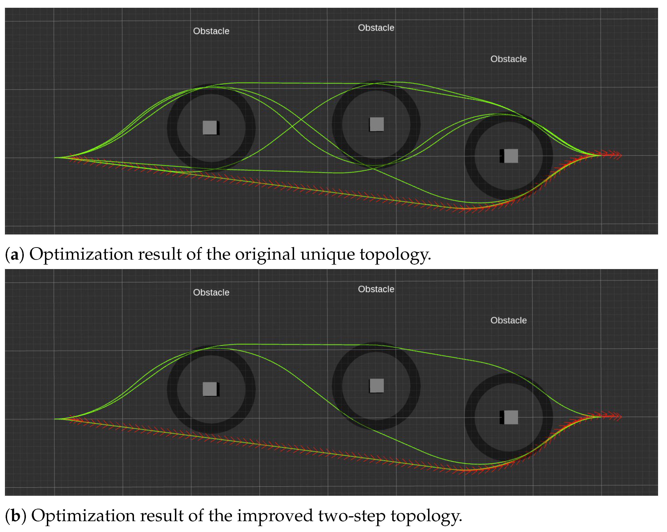
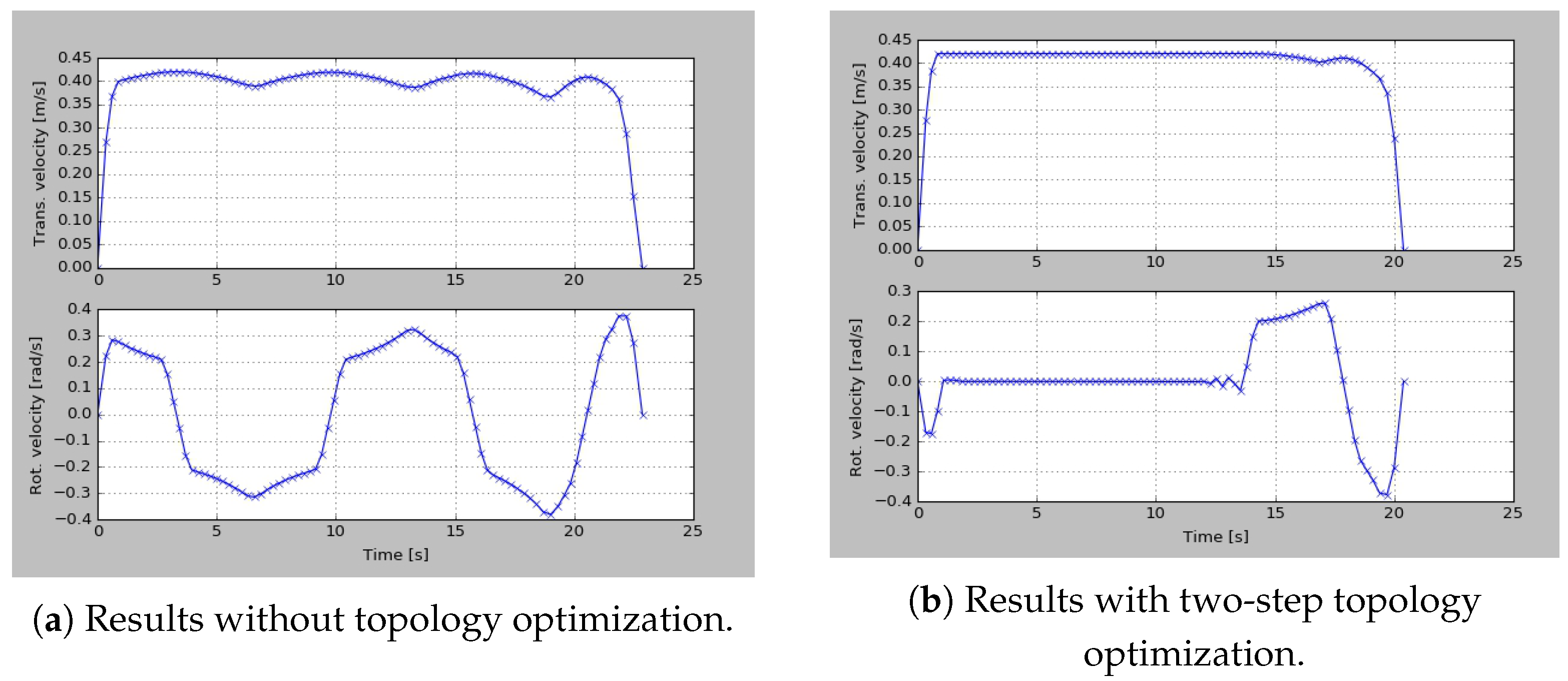
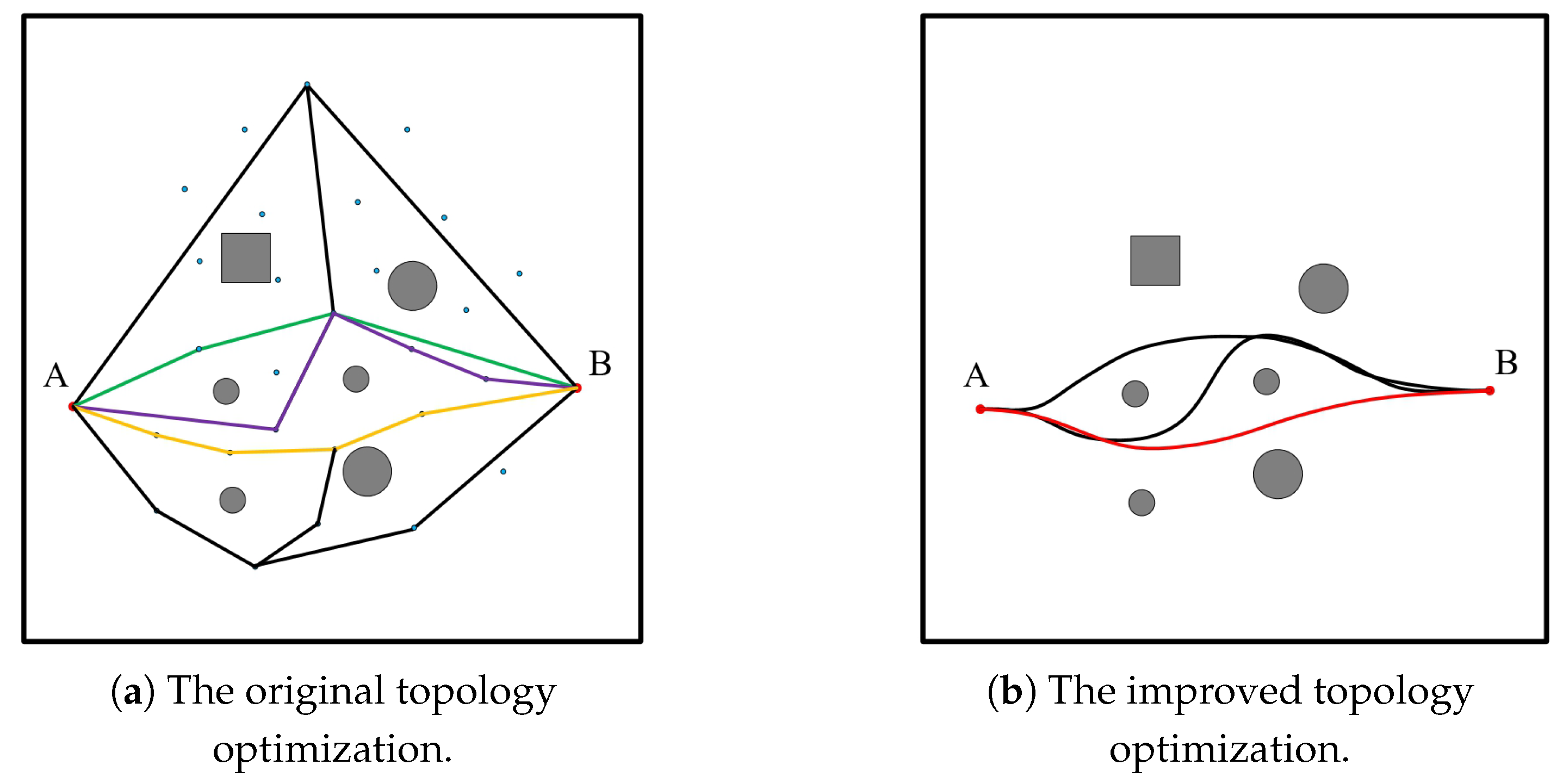
• An improved multiobjective local path topology optimization method based on the TEB is put forward to reduce the run time with better path smoothness simultaneously, which divides the process into path decision-making and speed decision-making.

The remainder of the paper is organized as follows. Section 2 presents the problem statements of path planning, RRT and TEB. Section 3 states the proposed path planning system to provide the details of MH-RRT and the improved two-step TEB. The validity simulations and real applicative experiments are explained in Section 4, as well as the comparisons with other traditional or state-art-of-work methods. Section 5 gives the conclusion and future work.

2. Preliminaries

In this section, we introduce the preliminaries about path planning problem and design criteria in Section 2.1, basic RRT algorithm in Section 2.2, and basic TEB algorithm in Section 2.3, respectively.

2.1. Path Planning Problem

In this paper, we take AGV as a differential drive mobile robot and address the path planning problem based on combining sampling-based with value-optimal based algorithms. Let x be the state, then $x_{init}$ and $x_{goal}$ present initial state and goal state. Obviously, $x_{start}\in \Omega$ and $x_{goal}\in \Omega$. Let $\Omega$ be the state space, ${\Omega }_{obs}$ the obstacle space, and ${\Omega }_{free}=\Omega -{\Omega }_{obs}$ the free space. Thus, the goal of path planning of AGV is to compute a feasible and safe trajectory $\sigma$: $[0,T]\to {\Omega }_{free}$ such that $\sigma \left(0\right)=x_{start}$, and $\sigma \left(T\right)=x_{goal}$.

The common path quality metrics are described below. Safety metric means minimum safe distance must be maintained. The length of path is defined as the sum of distances between all adjacent path points, and the shorter, the better. Besides, smoothness with smaller steering angles and real time with efficient computation are both essential quality metrics. We pay attention to these five metrics and evaluate our proposed method.

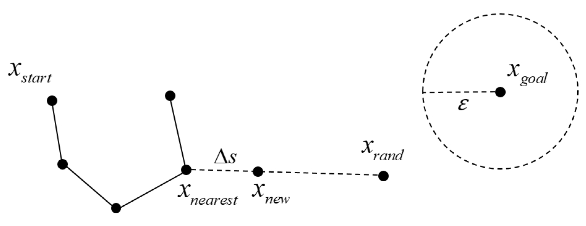
2.2. Rapidly Exploring Random Tree (RRT)

The RRT is devised to efficiently search the whole state space with a sampling scheme. We use x to denote the state information of a node, and use edge linked two nodes to denote the transition from one state to another. An illustration of the basic RRT algorithm is given in Figure 1. Given an initial position $x_{start}$ as the root of random tree T, the RRT planner iteratively samples a random sample node $x_{rand}$ from the state space. Then, it explores and selects the nearest node $x_{nearest}$ already in the tree to connect the sampled node $x_{rand}$ with a fixed incremental distance ${▵}_{step}$. If the distance between $x_{nearest}$ and $x_{rand}$ is larger than $ϵ$, $x_{rand}$ evolves as $x_{new}$. Next, a $CollisionFree$ function detects whether there is any obstacle lying between $x_{nearest}$ and $x_{new}$. If the collision detection succeeds, $x_{new}$ will be added as a vertex to the state tree T. An edge from $x_{near}$ to $x_{new}$ is also added. This loop lasts until the goal state $x_{goal}$ is found or the number of iteration reaches the threshold.

2.3. Timed Elastic Band (TEB)

The TEB is a local planner for on-line trajectory optimization. Building upon the work of Elastic Band (EB), the TEB approach incorporates temporal information directly into the optimization problem and thus accounts for the minimization of transition time under kinodynamic constraints. Let $Q={\left\{s_i\right\}}_{i=1,\dots ,n}$ denote a sequence of n poses $s_i=[x_i,y_i,{\beta }_i]\in R^2\times S^1$ linking together an initial and a final configuration, with $s_0$ fixed at the origin. The time interval required to transit from the current pose to the next pose is described as $\Delta T$. Let $\tau ={\{\Delta T_i\}}_{i=1,\dots ,n-1}$ denote a sequence of strictly positive time intervals. So TEB is defined by a tuple of parameters subject to optimization:

$$\begin{array}{c}\hfill B:=(Q,\tau )\end{array}$$

(1)

with the constraints such as initial $s_1$ and final configurations $s_n$, kinematics $h_i$ between two consecutive poses $s_i$ and $s_{i+1}$, limited translational velocity $v_i$ and acceleration $a_i$ and minimum clearance from obstacles $o_i$, the TEB optimization problem is formulated as a nonlinear program:

$$\begin{array}{c}\hfill \underset{B}{min}\sum _{i=1}^{n-1}\Delta T_i^2\end{array}$$

(2)

subject to

$$\begin{array}{c}\hfill \left\{\begin{array}{c}{\mathbf{s}}_1={\mathbf{s}}_s,{\mathbf{s}}_n={\mathbf{s}}_g,0\le \Delta T_i\le \Delta T_{max}\hfill \\ {\mathbf{h}}_i({\mathbf{s}}_{i+1},{\mathbf{s}}_i)=\mathbf{0},\hfill \\ {\mathbf{o}}_i\left({\mathbf{s}}_i\right)\ge \mathbf{0},\hfill \\ {\mathbf{v}}_i({\mathbf{s}}_{i+1},{\mathbf{s}}_i,\Delta T_i)\ge \mathbf{0},(i=1,2,...,n-1)\hfill \\ {\mathbf{a}}_i({\mathbf{s}}_{i+2},{\mathbf{s}}_{i+1},{\mathbf{s}}_i,\Delta T_{i+1},\Delta T_i)\ge \mathbf{0},(i=2,3,...,n-2)\hfill \\ {\mathbf{a}}_1({\mathbf{s}}_2,{\mathbf{s}}_1,\Delta T_i)\ge 0,{\mathbf{a}}_n({\mathbf{s}}_n,{\mathbf{s}}_{n-1},\Delta T_{n-1})\ge \mathbf{0}\hfill \end{array}\right.\end{array}$$

(3)

In Equation (3), $s_s$ is the current AGV state obtained from localization and $s_g$ denotes the goal state. $\Delta T$ is bounded from above to $\Delta T_{max}$ to accomplish an appropriate discretization of the continuous time motion, described in more detail in the following paragraphs. The TEB is illustrated in Figure 2.

The TEB approach further investigates the application of unconstrained optimization techniques. It utilizes Levenberg–Marquardt for solving this nonlinear least-squares problems due to its proper balance between robustness and efficiency. We adopt the optimized TEB with the g2o-framework based on hyper-graph. What is more, the TEB approach defines a closed-loop predictive control strategy in order to account for disturbances, map, and model uncertainties and dynamic environments that guides the AGV from its current state $s_s$ towards a goal state $s_g$. Since the resulting set of feasible poses is non-convex, the presence of obstacles introduces multiple local minima. Therefore, finding local minima coincides with the extraction of distinctive topologies. After obtaining many feasible candidate trajectories, homologous trajectories defined in [21] are removed by filtering. The non-homologous trajectories left are optimized in parallel, from which the local optimal path is selected.

While the trajectory is optimal, optimizing multiple paths at the same time requires high computing resources in practice. Sometimes the planning interval is much longer than the vehicle control interval, which cannot meet the real-time requirements of AGV. To deal with above issues, an improved two-step TEB is proposed. It is described in more details in the following section.

3. Methodology

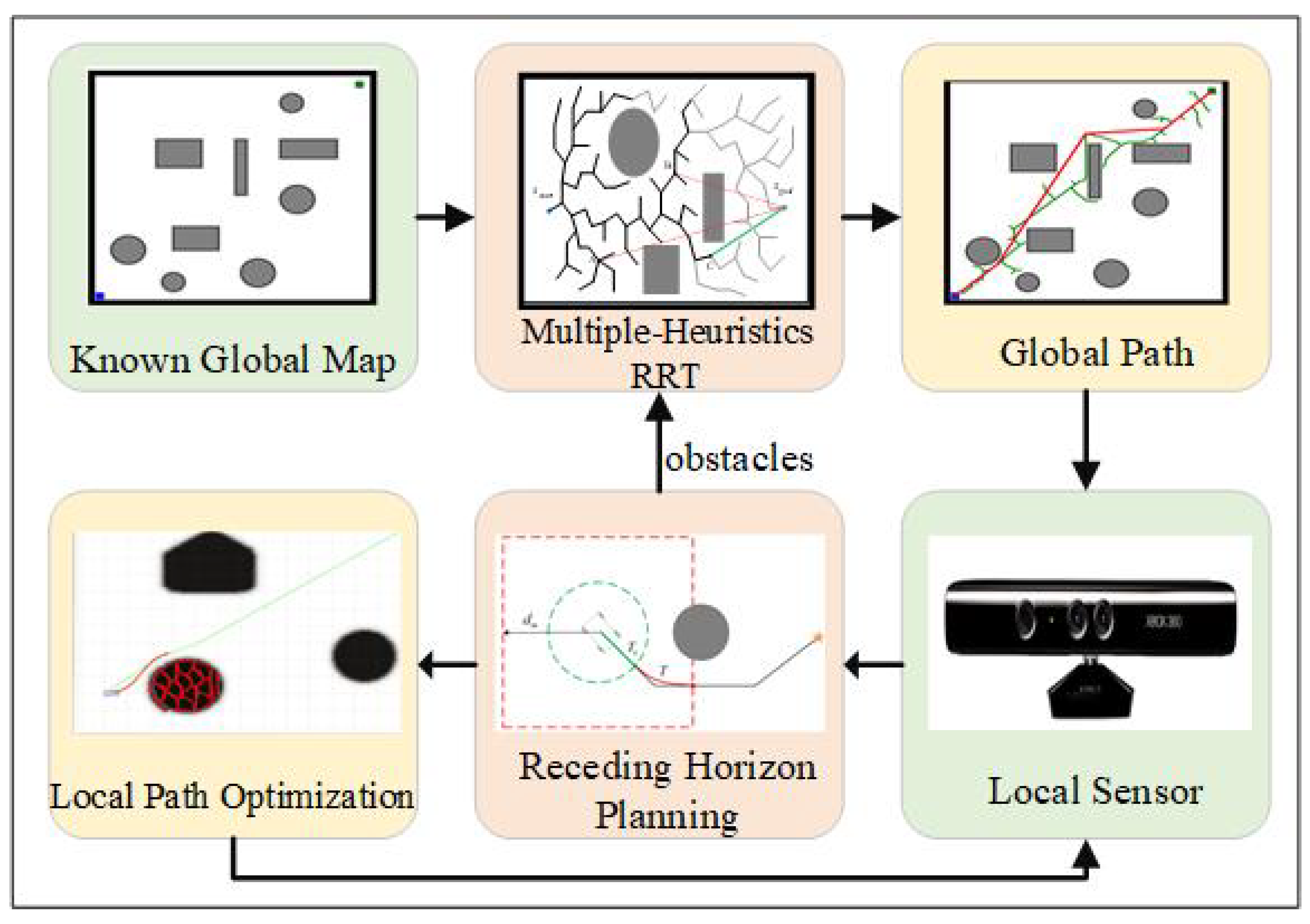
3.1. System Overview

In this section, a novel fusion method based on a global planner (MH-RRT) and a local planner (the improved TEB) is proposed for dynamic path planning. As is shown in Figure 3, the path planning system is composed of two main parts. At first, a modified RRT algorithm focuses on planning a feasible heuristic trajectory on the basis of the known global map. Then the improved TEB is responsible for optimizing the global trajectory after perceiving the local environment. The key point is utilizing the Receding Horizon Planning (RHP) to continuously generate local goal points until the AGV reaches the final goal. However, global planner will explore a new global trajectory when the local goal point is blocked by obstacles. Otherwise, the local path in sliding windows is optimized by the improved TEB and followed by control system in turn until arriving at the goal point. The proposed method is described as follows in detail.

3.2. Mutiple-Heuristics-RRT

In this section, the MH-RRT is proposed for dynamic path planning. The global path searching module is originated from RRT widely used for mobile robot. Yet, non-optimal, strong random and node redundancy are still unsolved. Aiming at above issues, we discuss a multiple-heuristics-RRT deployed five admissible and informative heuristics to speed up the searching in RRT. The main idea includes collision detection, goal-biased guidance, bidirectional extension, goal-point attempt and branch pruning strategy. The framework of the improved MH-RRT algorithm is presented in Algorithm 1.

Algorithm 1: Multiple-Heuristics-RRT

In the MH-RRT, the global path planning problem is formulated using the start state $x_{start}$, the goal state $x_{goal}$. Firstly, two trees, $T_1$, $T_2$ are initialized with the start state $x_{start}$ and the goal state $x_{goal}$, respectively. Secondly, a new state $x_{rand}$ is sampled randomly guided by goal point. Thirdly, the $Extend$ function taking into account the collision is used to guide the tree growth. What is more, a novel $GoalAttempt$ function is proposed to help the generated state try to link the final state with a certain probability. In each iteration, one tree is extended towards $x_{rand}$ followed by $GoalAttempt$ and the other tree makes attempt to connect the new state $x_{new}$. The roles are reversed by using the $Swap$ function. If the $Connect$ function finds that $T_2$ can reach the new state $x_{new}$ (e.g., there is no obstacle lying between the state $x_{new}$ and the state $x_2$ from $T_2$), the $GetPath$ function will find a broken line $P_{seg}$ connecting $T_2$ and $x_{new}$. That means two trees become connected and $Prune$ function is used to delete the edges with redundant turning point. Finally, a feasible path $P_{path}$ connecting $x_{start}$ and $x_{goal}$ is found. Otherwise, it reports $False$ when the global planner runs for the specified N iterations. Five heuristics are described as follows in detail.

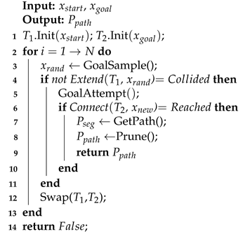
3.2.1. Collision Detection

In order to speed up the detection speed, we divide collision detection into two steps: rough detection and fine detection. Rough detection distinguish obstacles whether away from current state. And then it runs for further fine detection. Here, we adopt bounding boxes to present obstacles, the gaps between the bounding boxes and the obstacles can guarantee a safe distance. Thus, less computation time improves detection efficiency via two steps.

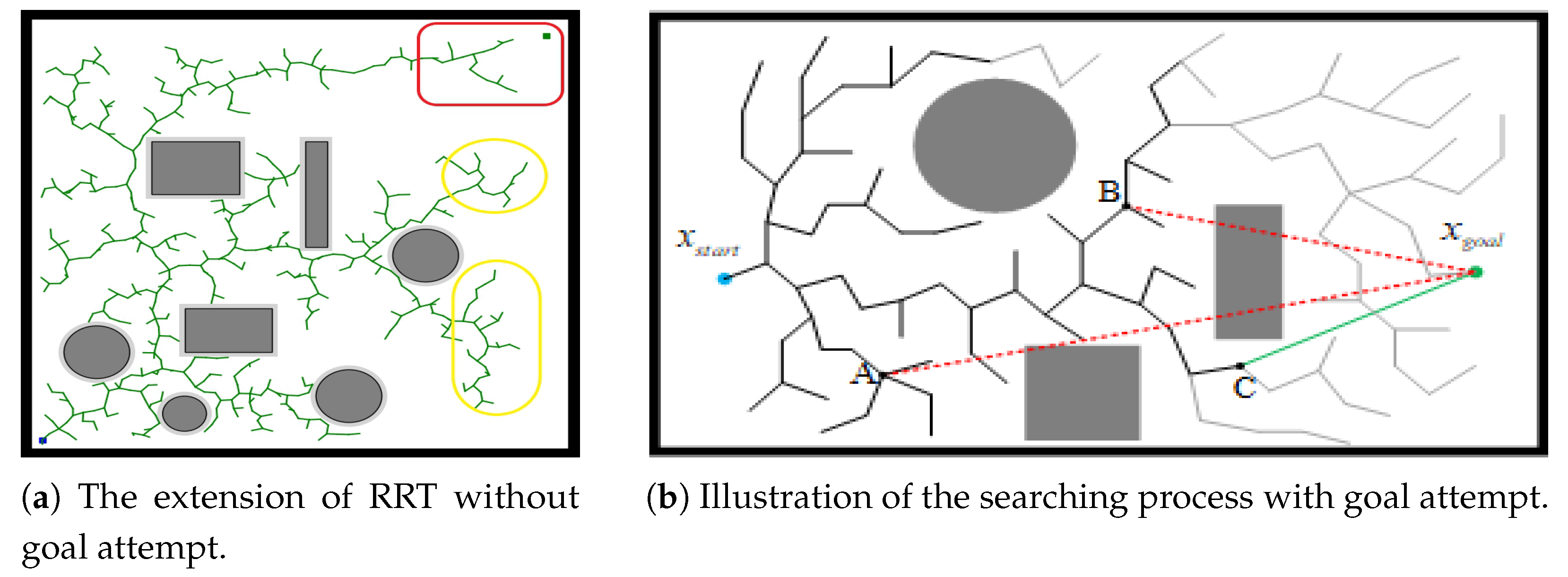
3.2.2. Goal-Biased Guidance

Aiming to reduce the exploration of invalid states, we combine RRT with the idea of goal-bias, which contributes to search efficiency [22]. With the goal-biased strategy, the improved RRT firstly presets a goal-biased probability named $p_0$ and a random probability based on uniformly samples named p. If $p>p_0$, it obtains a random state by uniformly sampling in configuration space, otherwise it sets the goal point $x_{goal}$ to next state $x_{rand}$. It is noted that $p_0$ usually less than 0.1 (0.1 in this paper), or state tree expands totally towards the target, leading to incomplete searching. The goal-biased strategy not only keeps the random property of the RRT algorithm, but also speeds up the convergence to the goal state.

3.2.3. Bi-Direction Extension

Bi-directional search method is a simple and effective idea to overcome the limitation that the number of states increases exponentially in large scale or complex environments [23]. The bi-directional RRT algorithm simultaneously expands two RRT trees towards each other from the start state $x_{start}$ and goal state $x_{goal}$, respectively. In each iteration, an attempt is made to connect the nearest vertex of the other tree to the new vertex after extending one tree. Then, the roles are reversed by swapping the two trees. When the distance between the nearest vertices of the two trees is less than the connection threshold, the two trees are considered to be close enough to be connected. The two trees are maintained all the time until they become connected and a solution path is found. With greedy heuristic, the idea of bi-direction extension not only benefits searching process but also keeps rapid and uniform exploration properties.

3.2.4. Goal-Point Attempt

Goal-point attempt is a novel heuristic rule which is proposed for solve issues as follows. Firstly, when current state is closed to the goal point as shown in Figure 4, it may take much more time to connect to the goal state due to random expansion. In addition, it is difficult to have a primitive end exactly in the goal state because of the discretized control input. Whenever a trajectory passes the collision and dynamic feasibility check, the searching is terminated in advance. The trajectory connects the current state $x_c$ to the goal state $x_g$ computed using the same approach in RRT. While it is uncertain, this strategy is effective especially in sparse environments. Since once it attempts successfully, it will terminate earlier and prevent the nodes hesitating to converge to the goal point.

As illustrated in Figure 4, black edges mean present exiting tree branches. The two red lines indicate that both state A and state B make goal attempt without success, owing to the rectangular obstacle. However, the green trajectory attempted from point C succeeds connecting to the goal point and the searching finished. What is more, the gray edges suggest next expansion branches if we continue searching without successful goal attempt. Thus, it can be seen a third of searching process is left out. Theoretically, attempting to connect to the goal costs extra computation to detect collision every time it searches. Besides, nodes far away from the destination are less likely to reach the goal point directly. Consequently, we investigate the goal-point attempt probability function as shown in Equation (4).

$$P\left(d\right)=\frac{\alpha }{1+e^d}+\lambda$$

(4)

Here we limit the probability less than $0.1$ to reduce the online computational burden and ensure sufficient trials. d denotes the distance from new state to goal point, and $L_m$ denotes total distance from start point to destination, and $P\left(d\right)$ shows the different probability. When d is small, new point and the goal point are only a short distance away which could employ a larger probability for successful attempt, while for points far away from the goal point, it is not necessary to try it frequently.

3.2.5. Branch Pruning

Too much redundant nodes cause longer and rough trajectory. Thus branch pruning strategy is introduced in our method as a heuristic for better global planning solution. After finding out a feasible path, all states have been generated by taking into account the above four heuristics. And then, the $Prune$ function will implement the branch pruning strategy. We take the start state as $x_A$ and check if collides from the goal point $x_{goal}$ as $x_B$. If the whole path from $x_A$ to $x_B$ does not intersect with any collision, those nodes are all deleted which locate between $x_A$ and $x_B$. Therefore, path with branch pruning has fewer nodes and curves. Furthermore, it is considered that pruning path is shorter and optimal from the trigonometric inequality. To summarize, collision detection guarantees the safety and feasibility of the path, while goal-biased guidance improves computation efficiency. Bi-direction extension mechanism guarantees that the connection between two adjacent states is optimal. Once goal attempt succeeds, the running time will be greatly reduced. Last but not the least, branch pruning brings smoother path. Improving the navie RRT with multiple heuristics will avoid redundant states and circuitous paths, contributing to high quality solution.

3.3. The Improved Two-Step TEB

Local path optimization is essential since the rough global path generated by the improved MH-RRT is hard for AGVs to track directly. TEB adopts topology optimization to all non-homologous paths at the same time after filtering homologous paths, which consumes much more computation resources. As a result, it sometimes cannot meet the real-time control requirements. On the basis of above problems, an improved two-step topology optimization strategy is proposed: path decision and speed decision. The pseudocode of two-step TEB local path planner is described in Algotithm 2.

Algorithm 2: Two-step Optimization

Similar to the original topology optimization, two-step topology optimization firstly selects non-homologous paths $P_{nh}$ from all sampled paths $P_s$. In contrast, we firstly sort all sampled paths $P_s$ and adopt the path decision to select only the first n paths. Sorting rules include both path length and distance to obstacles. Next, optimizing fewer rough trajectories instead of all non-homologous paths thus cost less computation.which have not been constrained by kinodynamic, thus cost less computation. The second step, speed decision, is optimizing the selected n paths considering TEB objective function including kinodynamic constrains. It seems like adding poses and time to these rough trajectories and deciding the AGV’s speed. Finally, compare these paths after optimization and choose the optimal one. In Figure 5, three chosen paths in different colors are better than others for AGVs to track. Aborting terrible paths and optimizing the good reduces unnecessary computation, and gets the optimal path as the naive topology optimization strategy does. To sum up, decision followed by optimization is superior to original optimization firstly. Rough paths decision provides initial solutions to speed decision, leading to computation efficiency and real-time control.

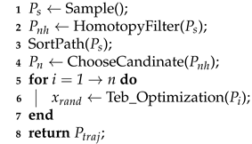
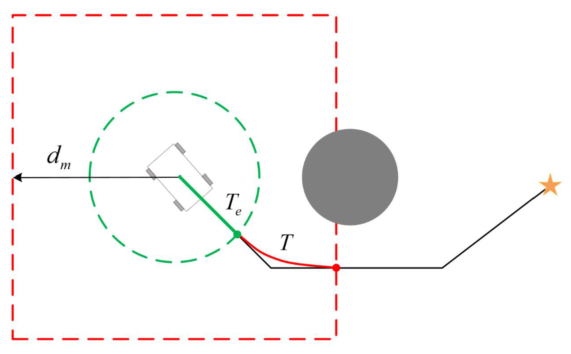
3.4. Receding Horizon Planning

When the AGV drives in an unknown environment, it has to follow the global path and optimize its local trajectory frequently due to the limited sensing range. To improve efficiency, a receding-horizon planning scheme is introduced. As illustrated in Figure 6, the five-point star denotes global goal point, while red intersection point means local goal point. Obviously, the local goal point is mostly not the goal point in global. The black curve connecting AGV to goal point is the global path generated by MH-RRT. $d_m$ presents the local planning distance limited by sensors, and here we use a square in a red dotted line to indicate the whole sensing range. Therefore, the local planner only optimizes trajectory in the square window, denoted as a red curve. Once AGV arrives at one local point and drives outside this range by control system, it drives into the next receding horizon window. If there is any obstacle lying on the path from AGV to the local goal point, it has to re-plan a global path by MH-RRT and repeat the above steps. In the square window, AGV can only follow part of local planning trajectory in fixed intervals, as the green curve in Figure 6. It indicates the start state of next local planning. Guided by the global path, the local planner does not stop running by horizon optimization recedes until AGV reaches the goal point. Then, the planning is successful and terminated. In our work, the re-planning is triggered in two situations. Firstly, it is called at fixed intervals of time to update the trajectory periodically using the most up-to-date environmental information. Secondly, it is triggered if the current trajectory collides with newly emergent obstacles, which ensures that a new safe global trajectory is available as soon as any collision is detected.

4. Simulation and Experiment

In this section, simulations and experiments are conducted to illustrate the feasibility and merit of the improved two algorithms. In the first simulation, the global path planning method MH-RRT is compared with other static path planning algorithms. Another simulation is conducted to validate the effectiveness of the proposed two-step TEB local planning algorithm in robot operating system (ROS) simulator Rviz. Specifically, each planner was executed 100 times for three different maps and results were compiled from these trials. What is more, the two algorithms combined by receding-horizon planning scheme are tested 30 times both in static and dynamic simulator environments. Simulations are conducted in Python, a computer with Intel Cure CPU i5-6500, 3.20 GHz, and 8-GB memory is used. Furthermore, the proposed complete path planner is applied on a robot (turtlebot2) for navigation to verify its effectiveness for challenging practical applications.

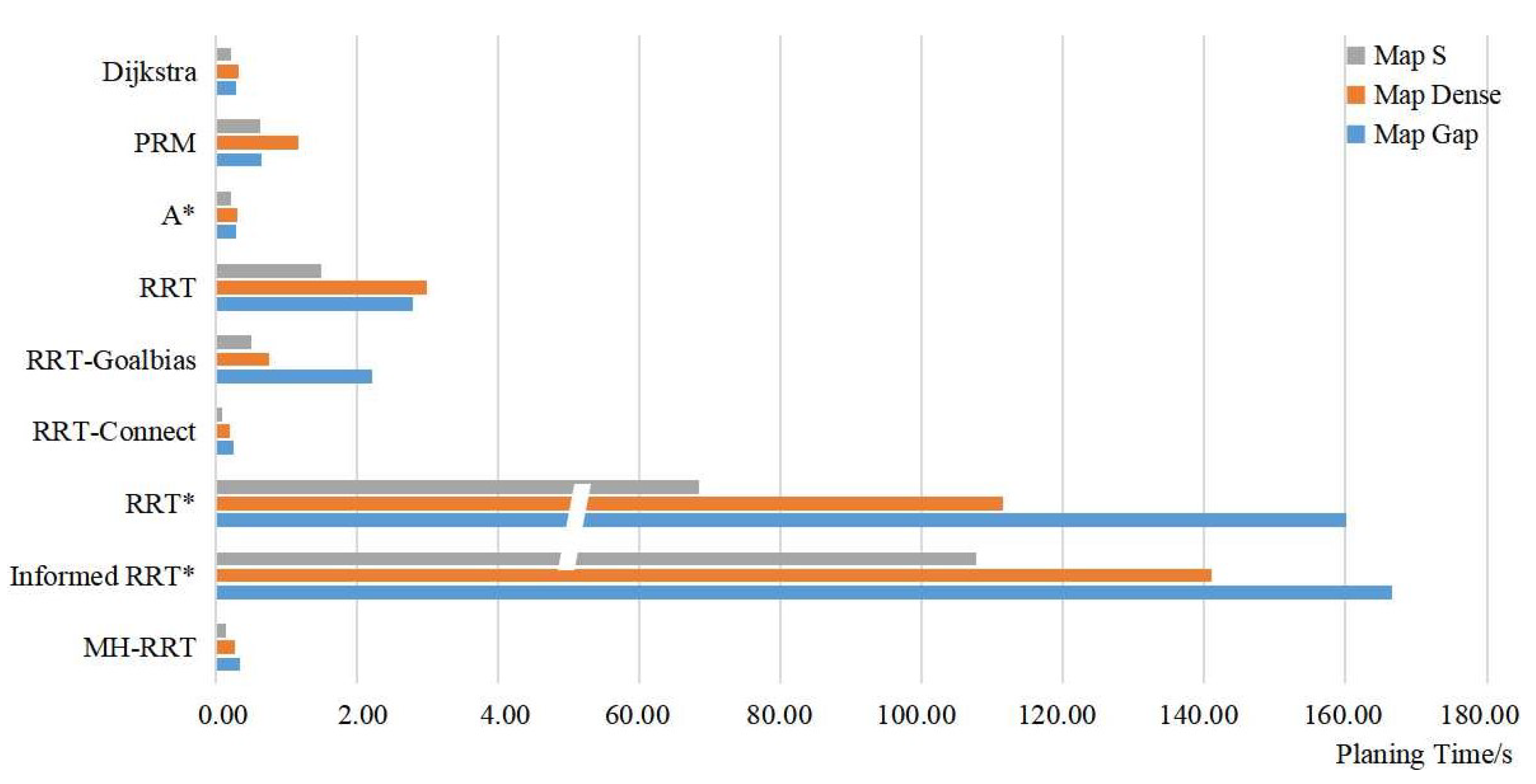
4.1. Comparison in Global Path Planning

The first simulation is conducted to validate the effectiveness of the improved MH-RRT in static path planning. Another eight path planning algorithms except the MH-RRT are compared in different metrics. Firstly, the naive RRT [11], RRT-Goal-biased [24], RRT-Connect [14], RRT* [16] and Informed RRT* [19] are selected for comparison, which are all the improvements of the RRT algorithm by inserting different heuristic functions. Besides, PRM [10] is selected which belongs to the same category as RRT. Lastly, two graph searching algorithms, Dijkstra [8] and A* [9], are chosen as another kind of path planning algorithm.

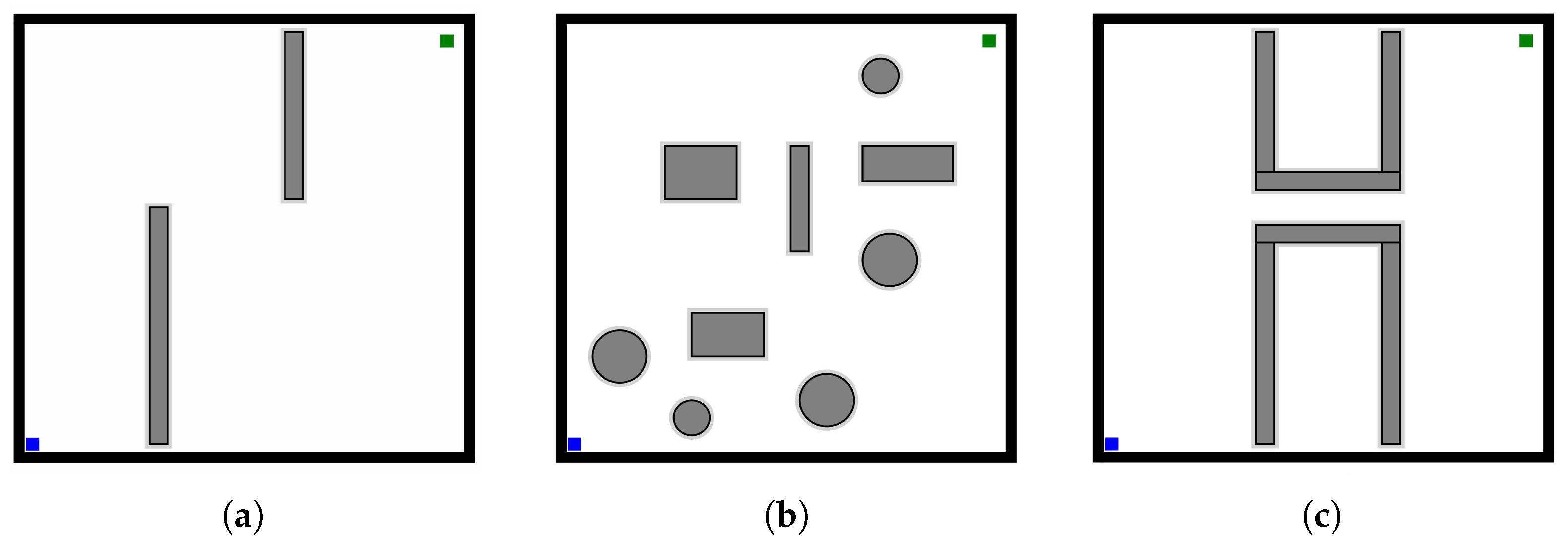
4.1.1. Simulation in Different Maps

As is shown in Figure 7, three maps are designed, called map S, map Dense and map Gap, and all map sizes are 50 × 50 m. Coordinates of start position and goal position are (2, 2) and (48, 48), respectively. The gray shadows around bounding boxes are expansion areas of obstacles. As the AGV is usually considered as a point, expanding the obstacles can guarantee safety to some extent. Here we adopt $0.5$ m by taking AGV’s size into consideration. Two indicators are used to evaluate the performance: Path length and execution time. The path length shows how far AGV moves to the goal. The planning time presents how long it takes to find out the global path.

As Figure 8 and Figure 9 show, the planning time of the MH-RRT, Dijkstra, A* and RRT-Connect planners in these three environments is well within realtime-capable requirements, with both less than 0.5 s, with a short advantage for RRT-Connect. For the path length metric, MH-RRT, RRT* and Informed RRT* perform very similar. Informed RRT* has a slightly lower value than the others but has much longer planning time. These first results highlight that the MH-RRT gives consideration to faster convergence speed and shorter path length. From comprehensive indications, the MH-RRT improves the quality of the generated paths.

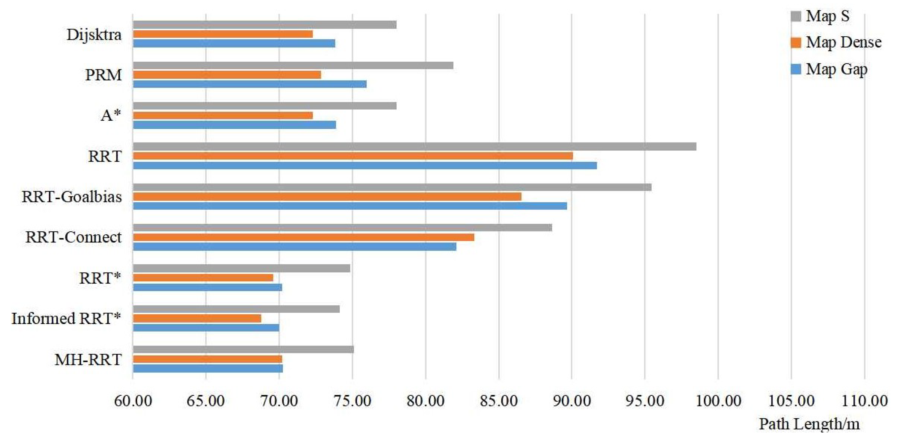
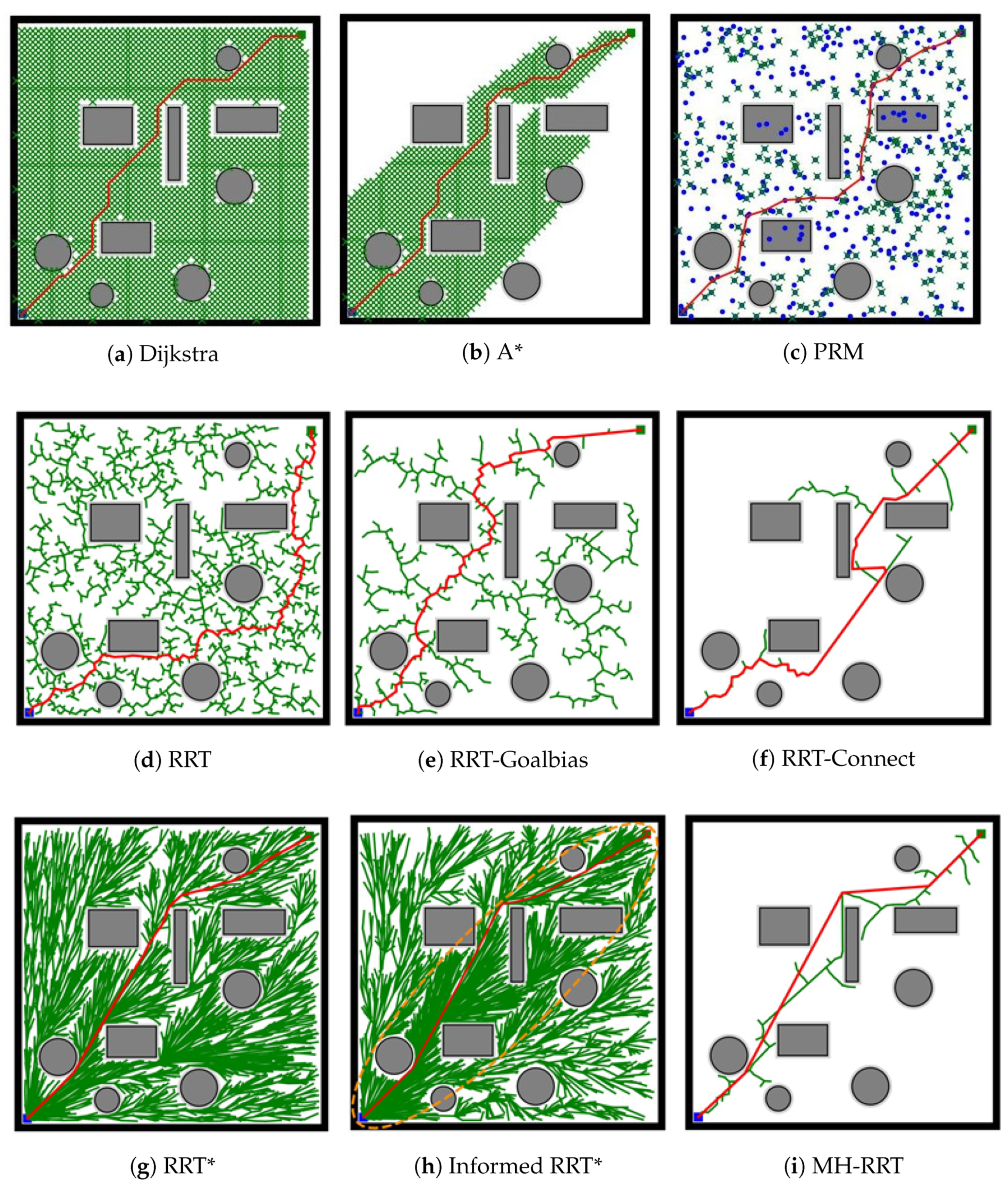
4.1.2. Comparison in Global Path

There are more obstacles surrounding the AGV in map Dense. Therefore, the results in map Dense are compared in detail. The evaluation covers another three metrics except path length and planning time. For RRT-based planners, the iteration times can effect the planning time, too. Moreover, the number of valid nodes or states in the searching tree indicates the smoothness of the trajectory’s curve. It is noted that Dijkstra, A* and PRM do not evaluate the above two metrics. Besides, the success rate declares whether the planner finds a collision-free trajectory or not. In each scenario, the execution is repeated 100 times.

Detailed results are listed in

Table 1. Experiment metrics.

	Planning	Path	Iteration	Valid	Success
	Time (s)	Length (m)	Times	Nodes	Rate
RRT	3.00	90.09	2271.63	92.13	100%
RRT-Goalbias	0.76	86.54	848.90	87.99	100%
RRT-Connect	0.20	83.35	216.66	84.04	100%
RRT*	111.46	69.57	5000.00	29.10	100%
Informed RRT*	140.98	68.76	5000.00	27.13	100%
Dijkstra	0.32	72.29			100%
A*	0.31	72.29	-	-	100%
PRM	1.17	72.86	-	-	100%
MH-RRT (ours)	0.28	70.19	208.70	6.70	100%

. It is obvious that the success rate of all seven sampling-based planners is 100%, due to complete probability. Besides, another two algorithms achieve complete success, too. However, the proposed MH-RRT executes fewer iteration times, which slightly increases computation efficiency. Figure 10 depicts the paths generated by the improved MH-RRT and other path planning algorithms. Observations for the number of MH-RRT path states are similar to RRT-Connect, while other RRT-based planners have many more branches. In addition, MH-RRT and Informed RRT* produce paths not only smoother but less prone to causing sudden motion. Note the path length (depicted in Figure 10) is a little shorter for MH-RRT than most of the paths, signifying better results.

4.2. Comparison in Local Path Planning

Without topology optimization, trajectory will be pressed down as the obstacle moves down. To better show the improvements of the proposed two-step TEB, Rviz, a ROS 3D robot visualizer, is used to simulate the algorithm’s optimization process. As shown in Figure 11, the two-step TEB (Figure 11b) computes the same trajectory as the naive TEB (Figure 11a). In contrast, the latter optimizes six paths while the former decreases to a half. The average time of original unique topology optimization process is 58.71 ms; however, the improved topology optimization process is 31.70 ms. Finally, two-step TEB outperforms naive TEB for computation time with 46% reduction. These results indicate the real-time property of the method.

The linear velocity and angular velocity metrics highlight the smoothness. Smoother trajectory requires less acceleration/deceleration. To validate the smoothness performance, experiments are conducted to compare with naive TEB. It is noted that the naive TEB optimizes path without any topology optimization. By the way, the linear velocity and angular velocity results shown in Figure 12b indicate the red curve in Figure 11b. Obviously, velocity improves to the max limited speed quickly with or without topology optimization. After that, the AGV travels keeping a constant speed and does not slow down sharply until it almost reaches the destination. In terms of Figure 12a, there are three deceleration points, at the moments 6.5 s, 13.1 s, and 18.9 s, respectively. It is common knowledge that vehicles decelerate when near the obstacles, thus understandably three deceleration points are due to three obstacles. However, only one deceleration point is proposed after adopting the two-step topology optimization category in Figure 12b. What is more, the bending complexity of the trajectory has a certain influence on the angular velocity. In the naive TEB angular velocity curve, the AGV has to turn a lot to follow the path as angular velocity varies greatly. Nevertheless, trajectory with improved topology optimization is smoother since angular velocity changes less.

Last but not the least, it is important to find solutions in a timely manner especially in the real applications. The trajectory time shows how long it takes to reach the goal. While it takes more time to optimize multiple paths, the two-step TEB can achieve planning within an AGV control period with enough computation resources. To sum up, the improved two-step TEB is, in terms of planning, more energy efficient and smoother than TEB with smaller average acceleration.

4.3. Results of the Proposed Fusion Algorithm

4.3.1. Simulation Results in Static Environment

The environment for static path planning simulation is a complex 2D map. There are eight known obstacles with black marks in the map. Coordinates of start position and goal position are blue mark (indicating the AGV) and green arrow which are chosen randomly, as shown in Figure 13.

By adopting the proposed fusion algorithm, AGV succeeds in finding out safe and smooth trajectories in thirty tests. Since there are similar results after 30 times, here one sample result is analyzed in detail. In Figure 13, the green global trajectory is composed of numerous path points. Red local trajectory includes locations and poses of the AGV. The obstacle locations are synthesized into convex polygons, which are presented by red mesh lines on the obstacles. Compared with taking obstacles as a set of points, it greatly improves the collision detection speed and reduces the optimization time. In the whole process, AGV drives smoothly and ensures a certain safe distance from the obstacles.

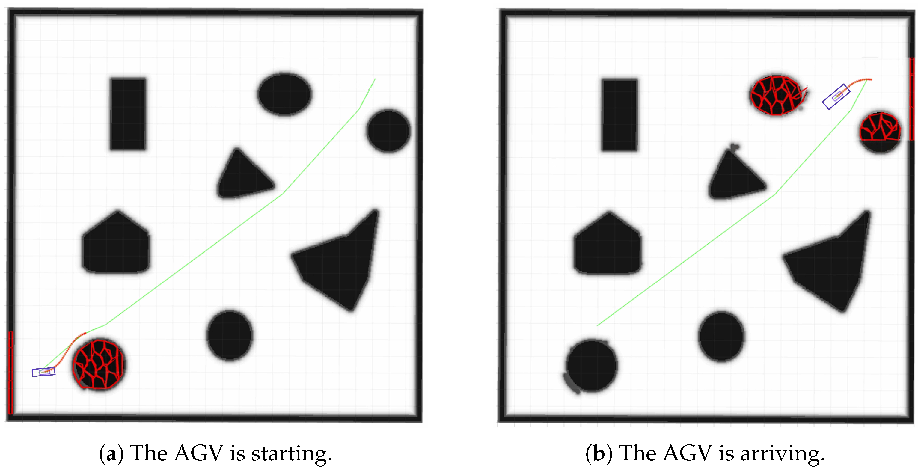
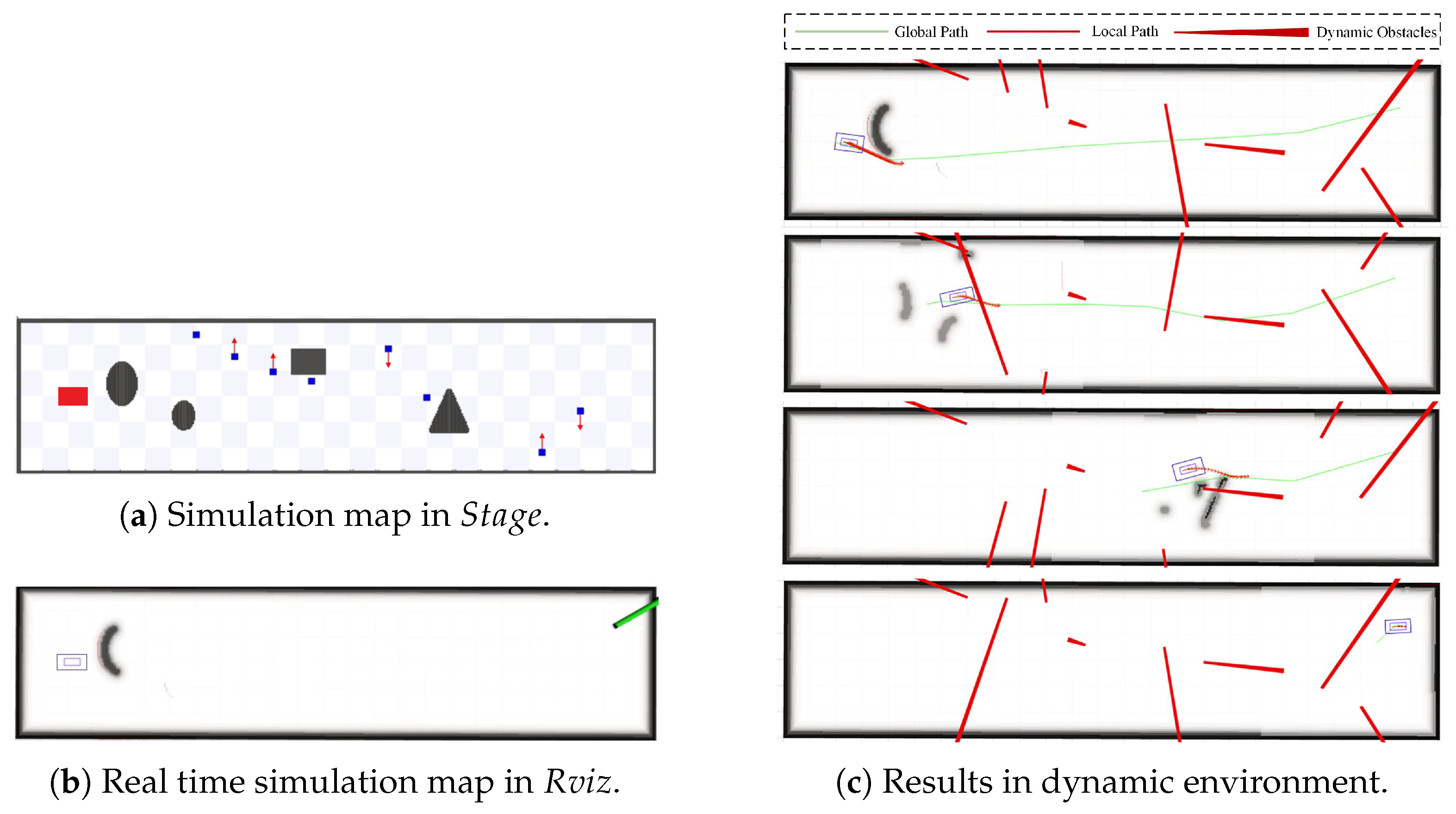
4.3.2. Simulation Results in Dynamic Environment

In this experiment, five dynamic AGVs and three static AGVs are added into the environment (shown in Figure 14a). The path planning AGV is presented by the red mark, while other AGVs are in blue. Red arrows indicate their running directions. When they arrive at the boundary, they turn back at the same speed. In Figure 14b, since the AGV can only sense specific distance ahead, there is only one gray arc obstacle in front of it. The green arrow indicates the destination pose. Except for the dynamic environment, other conditions such as static obstacles are designed the same as above. As depicted in Figure 14c, the AGV succeeds in avoiding every dynamic and static obstacle and reaches the goal point step by step.

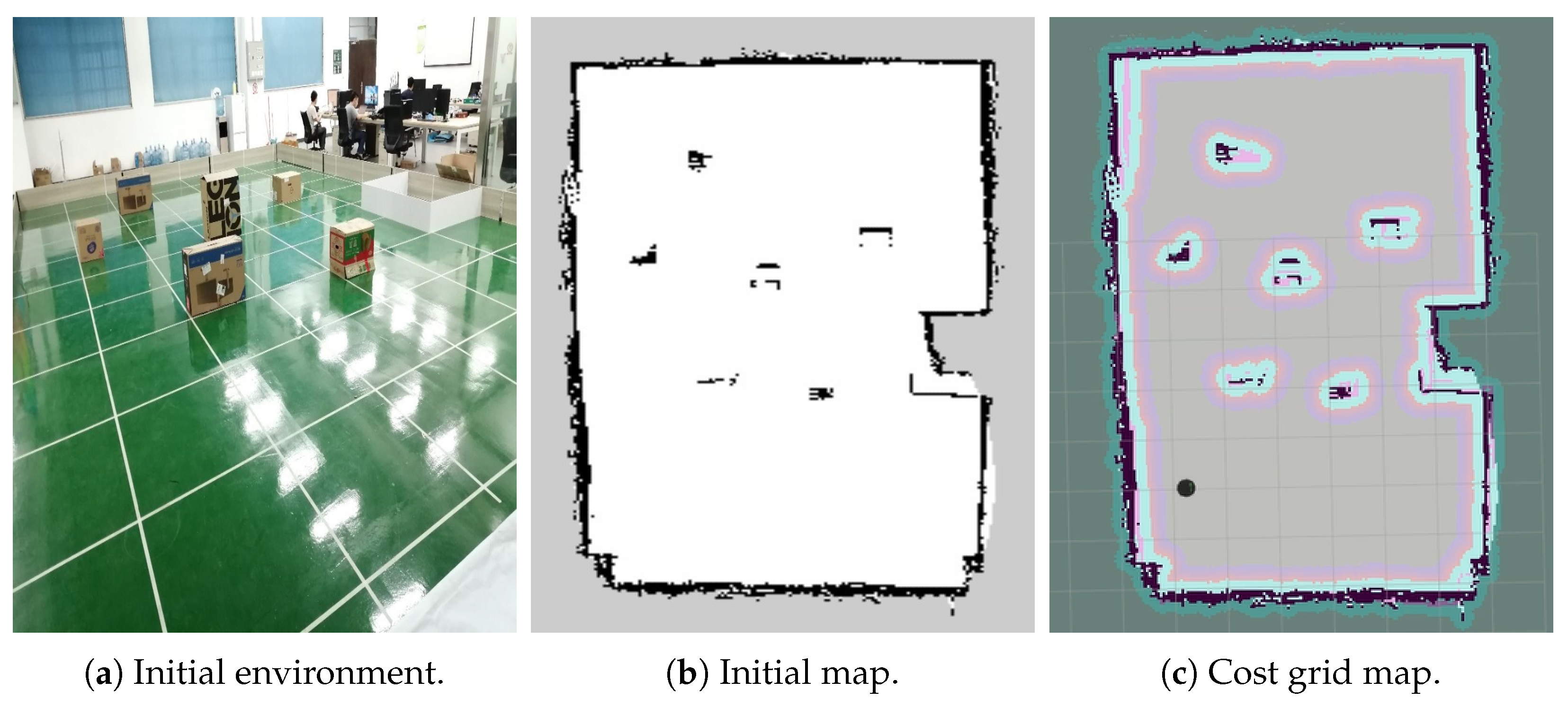
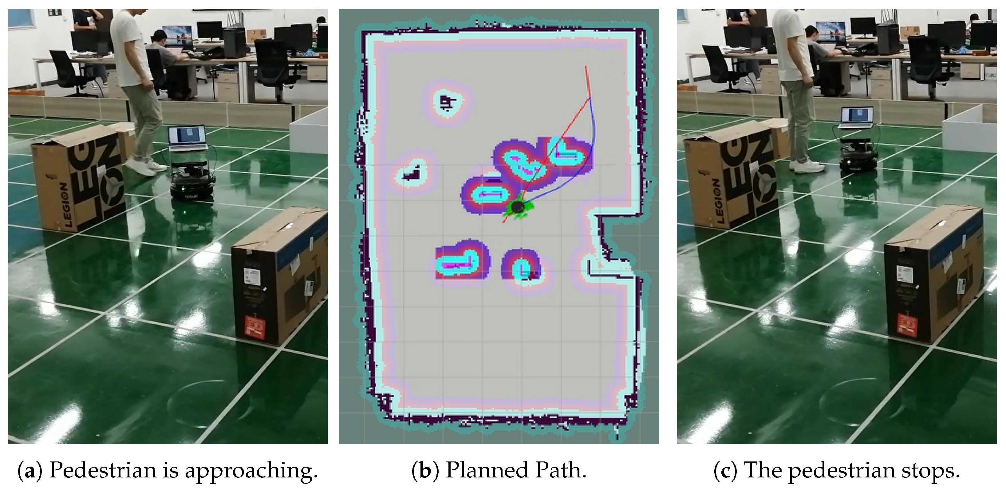
4.3.3. Real Experiment Results in Complex Dynamic Environments

The MH-RRT and two-step TEB are fused for further validation in real experiments. The hardware platform is the Turtlebot2 robot, which is one of the AGVs driven by the two differential driving wheels. It mainly includes a Yujin kobuki mobile base, a visual sensor named Kinect and the mechanical structure. In general, Kinect is a depth camera which is used to detect obstacles. Moreover, the robot operation system (ROS) is adopted as the software platform. ROS is a set of software libraries and tools that can help users build robot applications. The AGV is driven by a Lenovo notebook and complied with C++. The notebook equipped with ROS is responsible for mapping, location, and navigation. The linear velocity and angular velocity are constrained as $v\in (0,0.7 \mathrm{m}/\mathrm{s}]$ and $\omega \in [0,\pi \mathrm{r}\mathrm{a}\mathrm{d}/\mathrm{s}]$, respectively. Fused by receding horizon planning, the MH-RRT and two-step TEB algorithms are encapsulated as a path planner in ROS navigation package. As illustrated in Figure 15, the AGV generates a grid map (Figure 15b), and a cost grid map after expansion around obstacles (Figure 15c) on the basis of the initial environment (Figure 15a). Then the cost map is stored as the known map.

The AGV is placed at the start position indicated by a black circle. As for known dynamic obstacles, two kinds of walker are added to the environment sequentially. One is conservative, and the other is more aggressive who does not stop nearby the AGV. In the first situation, a pedestrian walks into the experimental field and stops when the AGV is travelling along the initial path. Figure 16 depicts the snapshots of the path planning with a conservative walker, it can be seen that the AGV successfully detects the walker and replans its path upgraded in map. Then it avoids the conservative walker. What is more, in Figure 17 the AGV decelerates appropriately and replans its path to bypass the aggressive walker. The experimental results show that the whole strategy is effective in practical applications.

5. Conclusions

In this paper, we propose a novel dynamic path planning method for AGV navigation. We decouple the dynamic path planning into global path searching and local path optimization. Firstly, a multiple heuristic strategy designed for the RRT can solve the problem of non-optimality. With five heuristics, the MH-RRT can reduce the iteration times especially by adopting the proposed goal attempt mechanism. Simulation shows that the MH-RRT can find a global optimal path within 210 iterations. Comparing with the other eight path planning algorithms, the MH-RRT can further find the shorter and smoother path. With this method, a feasible global path for AGV can be obtained. Next, we significantly improve the efficiency and converge rate of the two-step topology optimization in TEB. By utilizing the path decision and speed decision sequentially, the two-step TEB can optimize the local path in the receding horizon window. Finally, by fusing the above two planners with the receding horizon planning strategy, the effectiveness of the whole framework is verified both in simulation and real applicative experiments. Adequate ablation simulation experiments are also conducted for comparison. The results show the proposed fusion algorithm can achieve dynamic path planning and fast path optimization while avoiding obstacles. In the future, we plan to challenge the path planning system in extreme situations such as variable speed obstacles by adding a moving objects trajectory prediction system. Furthermore, we will combine the navigation system with a more complete autonomous perception system.

References

1. Ryck, M.; Versteyhe, M.; Debrouwere, F. Automated guided vehicle systems, state-of-the-art control algorithms and techniques. J. Manuf. Syst. 2020, 54, 152–173. [Google Scholar] [CrossRef]
2. Moshayedi, A.J.; Jinsong, L.; Liao, L. AGV (automated guided vehicle) robot: Mission and obstacles in design and performance. J. Simul. Anal. Nov. Technol. Mech. Eng. 2019, 12, 5–18. [Google Scholar]
3. Zhang, B.; Tang, L.; Decastro, J.; Roemer, M.J.; Goebel, K. A Recursive Receding Horizon Planning for Unmanned Vehicles. IEEE Trans. Ind. Electron. 2015, 62, 2912–2920. [Google Scholar] [CrossRef]
4. González, D.; Pérez, J.; Milanés, V.; Nashashibi, F. A Review of Motion Planning Techniques for Automated Vehicles. IEEE Trans. Intell. Transp. Syst. 2016, 17, 1135–1145. [Google Scholar] [CrossRef]
5. Reis, W.; Junior, O.M. Sensors applied to automated guided vehicle position control: A systematic literature review. Int. J. Adv. Manuf. Technol. 2021, 113, 21–34. [Google Scholar] [CrossRef]
6. Guang, X.; Guan, S.; Song, H. Research on Path Planning Based on Artificial Potential Field Algorithm. In Proceedings of the 2nd International Conference on Artificial Intelligence and Advanced Manufacture, Manchester, UK, 23–25 October 2020; pp. 125–129. [Google Scholar]
7. Sabudin, E.N.; Omar, R.; Joret, A.; Ponniran, A.; Debnath, S.K. Improved Potential Field Method for Robot Path Planning with Path Pruning. In Proceedings of the 11th National Technical Seminar on Unmanned System Technology 2019; Springer: Singapore, 2021. [Google Scholar]
8. Dijkstra, E.W. A note on two problems in connexion with graphs. Numer. Math. 1959, 1, 269–271. [Google Scholar] [CrossRef] [Green Version]
9. Hart, P.E.; Nilsson, N.J.; Raphael, B. A Formal Basis for the Heuristic Determination of Minimum Cost Paths. IEEE Trans. Syst. Sci. Cybern. 2007, 4, 100–107. [Google Scholar] [CrossRef]
10. Kavraki, L.E.; Svestka, P.; Latombe, J.C.; Overmars, M.H. Probabilistic Roadmaps for Path Planning in High-Dimensional Configuration Spaces. IEEE Trans. Robot. Autom. 1996, 12, 566–580. [Google Scholar] [CrossRef] [Green Version]
11. Lavalle, S.M. Rapidly Exploring Random Trees: A New Tool for Path Planning. 1998. Available online: https://www.cs.csustan.edu/~xliang/Courses/CS4710-21S/Papers/06%20RRT.pdf (accessed on 18 November 2021).
12. Lin, H.I. 2D-Span Resampling of Bi-RRT in Dynamic Path Planning. Int. J. Autom. Smart Technol. 2015, 4, 39–48. [Google Scholar] [CrossRef]
13. Qi, J.; Yang, H.; Sun, H. MOD-RRT*: A Sampling-Based Algorithm for Robot Path Planning in Dynamic Environment. IEEE Trans. Ind. Electron. 2020, 68, 7244–7251. [Google Scholar] [CrossRef]
14. Kuffner, J.J.; LaValle, S.M. RRT-connect: An efficient approach to single-query path planning. In Proceedings of the 2000 ICRA Millennium Conference, IEEE International Conference on Robotics and Automation. Symposia Proceedings (Cat. No. 00CH37065), San Francisco, CA, USA, 24–28 April 2000; Volume 2, pp. 995–1001. [Google Scholar]
15. Wang, J.; Meng, Q.H.; Khatib, O. EB-RRT: Optimal Motion Planning for Mobile Robots. IEEE Trans. Autom. Sci. Eng. 2020, 17, 2063–2073. [Google Scholar] [CrossRef]
16. Karaman, S.; Frazzoli, E. Sampling-based Algorithms for Optimal Motion Planning. Int. J. Robot. Res. 2011, 30, 846–894. [Google Scholar] [CrossRef]
17. Chen, L.; Shan, Y.; Tian, W.; Li, B.; Cao, D. A fast and efficient double-tree RRT*-like sampling-based planner applying on mobile robotic systems. IEEE/ASME Trans. Mechatron. 2018, 23, 2568–2578. [Google Scholar] [CrossRef]
18. Wang, J.; Li, B.; Meng, M.Q.H. Kinematic Constrained Bi-directional RRT with Efficient Branch Pruning for robot path planning. Expert Syst. Appl. 2021, 170, 114541. [Google Scholar] [CrossRef]
19. Gammell, J.D.; Srinivasa, S.S.; Barfoot, T.D. Informed RRT*: Optimal sampling-based path planning focused via direct sampling of an admissible ellipsoidal heuristic. In Proceedings of the 2014 IEEE/RSJ International Conference on Intelligent Robots and Systems, Chicago, IL, USA, 14–18 September 2014; pp. 2997–3004. [Google Scholar]
20. Rösmann, C.; Feiten, W.; Wösch, T.; Hoffmann, F.; Bertram, T. Trajectory modification considering dynamic constraints of autonomous robots. In Proceedings of the 7th German Conference on Robotics, Munich, Germany, 21–22 May 2012; pp. 1–6. [Google Scholar]
21. Bhattacharya, S. Topological and Geometric Techniques in Graph Search-Based Robot Planning; University of Pennsylvania: Philadelphia, PA, USA, 2012. [Google Scholar]
22. LaValle, S.M.; Kuffner, J.J., Jr. Randomized kinodynamic planning. Int. J. Robot. Res. 2001, 20, 378–400. [Google Scholar] [CrossRef]
23. Liu, H.; Zhang, X.; Wen, J.; Wang, R.; Chen, X. Goal-biased Bidirectional RRT based on Curve-smoothing. IFAC-PapersOnLine 2019, 52, 255–260. [Google Scholar] [CrossRef]
24. LaValle, S.M. Planning Algorithms; Cambridge University Press: Cambridge, UK, 2006. [Google Scholar]
Figure 1. Illustration of the sample and extension mechanism of the RRT algorithm.
Actuators 10 00314 g001
Figure 2. Illustration of the TEB algorithm. The TEB is a sequence of AGV poses forming a trajectory. Consecutive poses are tied to one another by a time interval.
Actuators 10 00314 g002
Figure 3. Illustration of the system overview. The path planning system is composed of two main parts: The global path planning and the local path optimization.
Actuators 10 00314 g003
Figure 4. Illustration of the searching process without/with goal attempt. In (a), states in red circle are very closed to the goal point. However it takes much more time to expand randomly, like redundant expansion in yellow circles. In (b), dotted lines in red mean failed attempts, while the green means it succeeds in connecting to the goal point.
Actuators 10 00314 g004
Figure 5. The topology optimization of the improved two-step TEB. A denotes the start point, and B denotes the goal point.The original TEB in (a) selects the top n; there are three paths from all sampled paths. The improved two-step TEB in (b) chooses the only optimal path after speed decision.
Actuators 10 00314 g005
Figure 6. The combination planning strategy for a limited sensing range. The black curve and the red curve are the trajectories before and after the optimization. Circular obstacles are known.
Actuators 10 00314 g006
Figure 7. Three different maps. The start position is denoted as a blue point while the goal is green. (a) Map S.; (b) Map Dense.; (c) Map Gap.
Actuators 10 00314 g007
Figure 8. Result of planning time for the nine algorithms in three maps.
Actuators 10 00314 g008
Figure 9. Results of path length for the nine algorithms in three maps.
Actuators 10 00314 g009
Figure 10. Illustration of nine global path planning results in map Dense. In (a,b), the green grids indicate that these grids have been searched. In (c), the green crosses indicate that these points have been sampled. In (di), the green curves denote the state tree structure. In all subfigures, the red line means the final path. All experiments start from the bottom left (marked in blue), and end at the top right (marked in green).
Actuators 10 00314 g010
Figure 11. The results of trajectory optimization. In both (a,b), three small gray cube obstacles are placed in Rviz. The black circle around the obstacle indicates the minimum safe distance between AGV and the obstacle. The red line is the optimal trajectory, including the position and attitude of each point.
Actuators 10 00314 g011
Figure 12. Linear velocity and angular velocity results of the optimal trajectories.
Actuators 10 00314 g012
Figure 13. Illustration fused results of global path generating and local path planning in simulation static environment. Initial global path and optimized local trajectory are drawn in green and red to distinguish them. Blue mark presents the AGV, whose kinematic model has been described in Section 2.3.
Actuators 10 00314 g013
Figure 14. Simulation maps in dynamic environment. In (c), global trajectories and real-time local paths are drawn in green and red colors to distinguish. Here we just draw robots driving direction in red instead of robots shape. Blocks in black present obstacles within sensing range.
Actuators 10 00314 g014
Figure 15. Initial environment and its cost grid map before/after expansion.
Actuators 10 00314 g015
Figure 16. Snapshots of path planning in dynamic situation with a conservative walker.
Actuators 10 00314 g016
Figure 17. Snapshots of path planning in dynamic situation with an aggressive walker.
Actuators 10 00314 g017