Constrained Path Planning for Unmanned Aerial Vehicle in 3D Terrain Using Modified Multi-Objective Particle Swarm Optimization

Abstract

This paper considered the constrained unmanned aerial vehicle (UAV) path planning problem as the multi-objective optimization problem, in which both costs and constraints are treated as the objective functions. A novel multi-objective particle swarm optimization algorithm based on the Gaussian distribution and the Q-Learning technique (GMOPSO-QL) is proposed and applied to determine the feasible and optimal path for UAV. In GMOPSO-QL, the Gaussian distribution based updating operator is adopted to generate new particles, and the exploration and exploitation modes are introduced to enhance population diversity and convergence speed, respectively. Moreover, the Q-Learning based mode selection logic is introduced to balance the global search with the local search in the evolution process. Simulation results indicate that our proposed GMOPSO-QL can deal with the constrained UAV path planning problem and is superior to existing optimization algorithms in terms of efficiency and robustness.

1. Introduction

The unmanned aerial vehicle (UAV) is a kind of aircraft without a human pilot, which is widely used in commercial, agricultural, military, and other fields [1,2,3]. Path planning is one of the most basic problems in the UAV flight management system, of which the purpose is to design a safe and short enough trajectory linking the starting and target points and satisfying some constraints [4,5,6]. Taking UAV flight distance and risk as objective functions, the height of UAV, angle of UAV, and limited UAV slope as constraints, Yu et al. [7] established an optimization model, which was solved by an adaptive selective mutation constrained differential evolution algorithm. Liu et al. [8] proposed a four-dimensional coordinated collision free path planning method for multiple UAVs, which took time variables into account and successfully generated collision free paths for multiple UAVs with the same time consumption. Maw et al. [9] proposed a hybrid path planning algorithm, which adopted an anytime graph-based path planning algorithm for global planning and deep reinforcement learning for local planning. This real-time mission planning system applied to autonomous UAV can adapt to the real environment and effectively avoid both static and moving obstacles.

The commonly used constraint-handling technique is the penalty function method [10], which constructs a new objective function by adding constraints to the original objective function and thus transfers the constrained optimization problem into the unconstrained one. Besides, the feasibility rule proposed by Deb [11] is another popular constraint-handling technique. By comparing individuals in pairs with three comparison rules, it chooses the better ones to keep to the next generation. Furthermore, multi-objective optimization approaches can also be employed to handle these constrained problems [12,13] by treating the cost and constraint conditions as the objective functions simultaneously.

Recently, various meta-heuristic algorithms were proposed to solve optimization problems, including particle swarm optimization (PSO) [14], pigeon-inspired optimization (PIO) [15], differential evolution (DE) [16], ant colony optimization (ACO) [17], fruit fly optimization algorithm (FOA) [18], and so on. Due to its simplicity and rapid convergence, PSO is the popular meta-heuristic algorithm in the multi-objective domain. At present, the multi-objective PSO (MOPSO) and its variants have been widely used in electromagnetic problems [19], vehicle scheduling [20], service allocation [21], and path planning [22].

Q-Learning is a method of reinforcement learning in the branch of machine learning, which has good performance in solving Markov decision process with an unknown environment model [23]. Its advantage lies in simple calculation, easy implementation, and self-improvement through reward and punishment measures [24]. Q-Learning chooses the appropriate next action by updating the state-action table with reward values. In this paper, we propose a Gaussian-based multi-objective particle swarm optimization algorithm with Q-Learning (GMOPSO-QL), which was applied to solve the offline UAV path planning problem.

The main contributions and innovations of this paper include the following aspects:

(1) The constrained UAV path planning problem is modeled as a multi-objective optimization problem, where the objective functions include not only the flight length and altitude cost objectives, but also the threat, terrain, turning, climbing and gliding constraint objectives, and the MPSO technology is employed herein to find a good and feasible path which satisfies the constraints.

(2) To overcome the drawback in which the original MOPSO often falls into the local optimal solutions in solving the complex UAV path planning problem, a novel Gaussian distribution-based velocity operator is adopted to compute the update the velocity of particles, which can effectively enhance the anti-premature ability, the search capability, and the convergence rate of the optimization algorithm.

(3) Two searching modes, the exploitation mode and the exploration mode, are designed for particles to update their states. Based on the Q-Learning strategy, each particle can choose the more effective searching mode for itself according to its own current status, so that the particles can achieve the more powerful and robust global optimization ability.

The proposed GMOPSO-QL is tested to find the best and feasible flight path for UAV in different 3D terrain mission scenarios, and the comparative results demonstrate the superior performance of our proposed GMOPSO-QL algorithm to the original MOPSO and GMOPSO method in solving the UAV path planning problem.

The overall structure of this paper is organized as follows. Section 2 presents the related works, including a brief introduction to MOPSO and Q-Learning. In Section 3, a modified GMOPSO-QL algorithm is proposed. In Section 4, the path planning based on the proposed algorithm is described in detail, including problem modelling and the planning process. Related simulation results are provided in Section 5. Section 6 finally summarizes this paper.

2. Related Work

2.1. Basic MOPSO

For a multi-objective optimization problem, it is extremely difficult and important to increase the solution diversity. Researchers first extended the PSO strategy to solve multi-objective problems [25]. It introduces the concept of external archives and adopts the non-dominant solution in archives to guide the search direction of particles, which keeps the population diversity. The speed update formula of particles is modified as follows [25]:

$$v_i(t+1)=\omega \cdot v_i(t)+c_1\cdot r_1\cdot (x_{\mathrm{pbest},i}(t)-x_i(t))+c_2\cdot r_2\cdot (x_{\mathrm{gbest}}(t)-x_i(t))$$

(1)

$$x_i(t+1)=x_i(t)+v_i(t+1)$$

(2)

where t represents iteration count; ω represents the inertia factor; c₁, c₂ represent learning factors; r₁, r₂ are uniformly generated random numbers in [0, 1]; x_gbest denotes a random particle in the archives; x_pbest,i denotes the historical optimal location for the i-th particle.

The implementation process of MOPSO can be described as Algorithm 1.

Algorithm 1. The structure of MOPSO
	/*Initialization*/
	Set the iteration count t = 1.
	Initialize the location xi and velocities vi of particles randomly, i = 1,2,…,NP.
	/*Establish archives*/
	Non-dominated sorting and save non-dominated solutions to archives A.
	/*Iteration computation*/
	while t < tmax do
		for each particle i do
			Update the velocity vi and position xi by Equations (1) and (2).
			Update the personal best position xpbest,i.
		end for
		/*Update archives*/
		if  the non-dominated solution generated in this iteration dominates the solution in the external archives, then delete the dominated solution.
		if  the non-dominated solution generated in this iteration is not dominated by any solution in the archives A, then place it in the archives A.
		if  the capacity of archives A exceed the maximum capacity requirement, then calculate the crowding distance of all individuals in the archives A and arrange them in descending order. Delete the individuals with the smallest crowding distance one by one until the capacity of archives A is equal to the maximum capacity.
		t = t + 1.
	end while

2.2. Q-Learning

Reinforcement learning is where an agent learns in a “trial and error” manner, and rewards are obtained through interaction with the environment guiding its behavior [24]. Q-Learning is one of the more commonly used algorithms in reinforcement learning at present, used mainly to learn how to choose the action that can generate the largest accumulated reward value through rewarding or punishing.

Q-Learning involves an agent, state set S, and action set A. By performing actions in the environment that cause the agent to transition from one state to another, performing actions in a specific state provides rewards. In short, Q(s,a) is the expectation of rewards that can be obtained by taking action a (a∈A) in the state of s (s∈S) at a certain moment. For Q-Learning, a Q-table is constructed by combining state s and action a, and then the optimal action is chosen based on the Q-value. Finally, the Q-table is updated through reward or punishment. Therefore, the core idea of Q-Learning is to get the optimal control strategy by maximizing rewards. For multiple iterations, the Q-table is updated dynamically as follows:

$$Q\left(s_t,a_t\right)\leftarrow Q\left(s_t,a_t\right)+\lambda \left[r_{t+1}+\gamma \underset{a}{max}Q\left(s_{t+1},a\right)-Q\left(s_t,a_t\right)\right]$$

(3)

where γ stands for the discount factor; λ is the learning rate; r_t+1 denotes the immediate reward obtained from the performance of a_t at the state s_t.

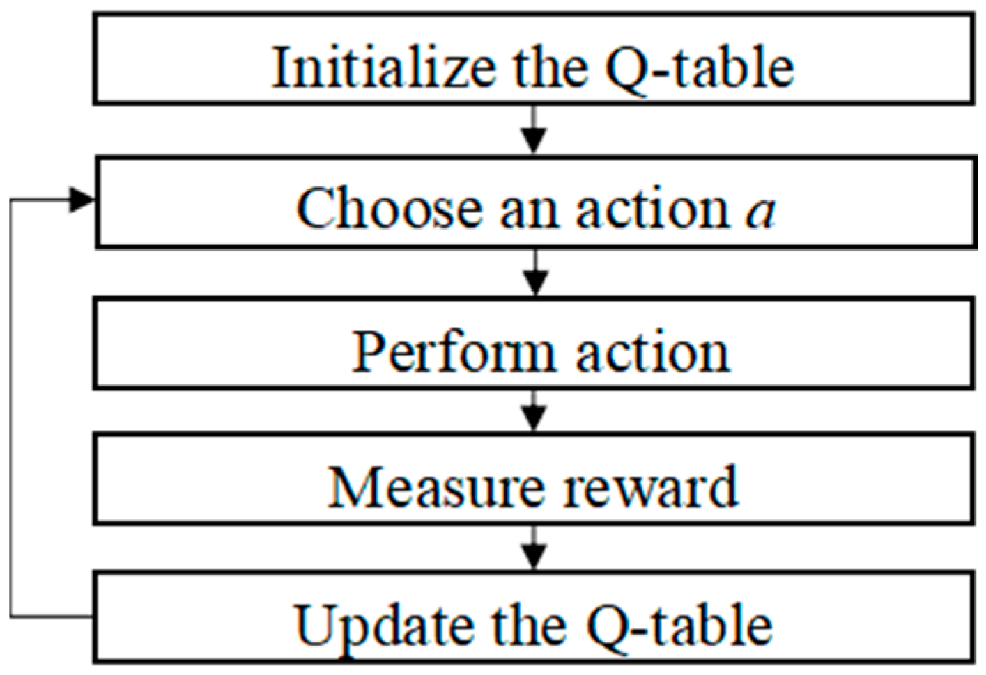
Figure 1 displays the structure diagram of Q-Learning.

3. Proposed Modified Algorithm

Global and local searches play significant roles in solving complex optimization problems. However, it is difficult to consider both of them in a single search mode. Introducing Q-Learning can solve this problem well. In this paper, two search modes are adopted, in which one tends to focus on global search, and the other focuses more on local search. Based on the learned experience, it constantly chooses one of them to complete the search process. Therefore, the balance of global and local search processes can be realized well.

3.1. Gaussian Based Exploration and Exploitation Update Modes

The contradiction between global search ability and local search ability restricts the performance of the algorithm. In GMOPSO-QL, the exploration mode performs a global search to find the possible range of the optimal solution. In contrast, the exploitation mode performs a local search to find the optimal solution within the possible range.

Equation (1) is the velocity update method of particles applied to the single-objective optimization problem. In the formula, x_gbest is the global optimal solution. However, it is replaced by a set of solutions, saved in the external archives, in the multi-objective optimization problem. Meanwhile, to enhance the randomness of basic MOPSO, Gaussian random number is employed to replace the commonly used uniformly distributed random numbers, which performs better in many cases [26]. Therefore, a speed update operator with Gaussian distribution is adopted to modify Equation (1). Then, the velocity update method of the particles in the exploration and exploitation update mode is obtained as follows:

(1) Exploration update mode

$$v_i\left(t+1\right)=\omega \cdot v_i+c_{11}\cdot r_1\cdot (x_{\mathrm{pbest},i}\left(t\right)-x_i(t\left)\right)+c_{21}\cdot g_1\cdot (x_{\mathrm{b}}\left(t\right)-x_i(t\left)\right)$$

(4)

where x_b is a random individual in the external archives, and g₁ is generated with Gaussian distribution. The learning factor c₁₁ should be large and c₂₁ should be small, so that the historical experience of the particles themselves can more mainly guide the search direction and enhance the diversity of the population.

(2) Exploitation update mode

$$v_i\left(t+1\right)=\omega \cdot v_i+c_{12}\cdot r_1\cdot (x_{\mathrm{pbest},i}\left(t\right)-x_i(t\left)\right)+c_{22}\cdot g_1\cdot (x_{\mathrm{b}}\left(t\right)-x_i(t\left)\right)$$

(5)

where the learning factor c₁₂ should be small and c₂₂ should be large, so that the optimal particles can guide the search direction more, and the algorithm can converge to the optimal solution more quickly.

3.2. Q-Learning Based Mode Selection

Q-Learning is used to select two update modes, which are exploration update mode and exploitation update mode. They share the same formula form but differ in the size of the learning factors. The exploration update mode has large c₁ and small c₂, so that the historical experience of particles themselves can guide the search direction more, thus enhancing the population diversity. As opposed to the exploration update mode, the exploitation update mode has a small c₁ and a large c₂. This allows the optimal particle to guide the search direction more and the algorithm to converge quickly.

In the proposed algorithm, each individual has its own Q-table to ensure that the learning process being independent. The Q-table is designed as a 2 × 2 matrix with the columns representing actions and rows representing states. When the update mode is chosen, the action corresponding to the largest Q-value in the current “state” line is the update mode of the particle position in this iteration.

In the Q-Learning algorithm, the setting of the learning rate λ is very important [24]. When it is close to 1, the agent will consider future rewards with greater weight; when it is close to 0, the agent tends to only consider immediate rewards. Therefore, the learning rate can be adaptively reduced during the iterative process, which can effectively learn from the search space [27].

In this paper, the learning rate is updated as follows:

$$\lambda =\frac{{\lambda }_{initial}+{\lambda }_{final}}{2}-\frac{{\lambda }_{initial}-{\lambda }_{final}}{2}\cdot \cos \left(\pi \left(1-\frac{t}{t_{max}}\right)\right)$$

(6)

where λ_initial and λ_final are the initial and final values of λ, respectively; t_max denotes the maximum number of iterations.

The reward r is calculated as follows:

$$r=\left\{\begin{array}{l}1\hspace{1em}\mathrm{if}\hspace{1em}\mathrm{the}\hspace{1em}\mathrm{fitness}\hspace{1em}\mathrm{is}\hspace{1em}\mathrm{improved}\hfill \\ -1\hspace{1em}\mathrm{otherwise}\hfill \end{array}\right.$$

(7)

3.3. Updating Archives

The external archives are adopted to store the non-dominated solutions resulting from the search process. At the end of the search, the external archives are the final optimal solution set. The update strategy for external archives is shown in Algorithm 2.

Algorithm 2. Steps of updating external archives
	/*Input parameters*/
	The current capacity of external archives m, the maximum capacity of external archives M
	/*Update Archives*/
	For each particle in current population xi do
		For each particle in the archives xj do
			If xi dominates xj do
				Delete xj from the archives
			End if
		End for
		If xi is not dominated by any solution in the archives do
			Place xi in the archives.
		End if
	End for
	If m > Mdo
		Calculate the crowding distance of all solutions in the archives and arrange them in descending order.
		Delete the solutions with the smaller crowding distance until m = M.
	End if

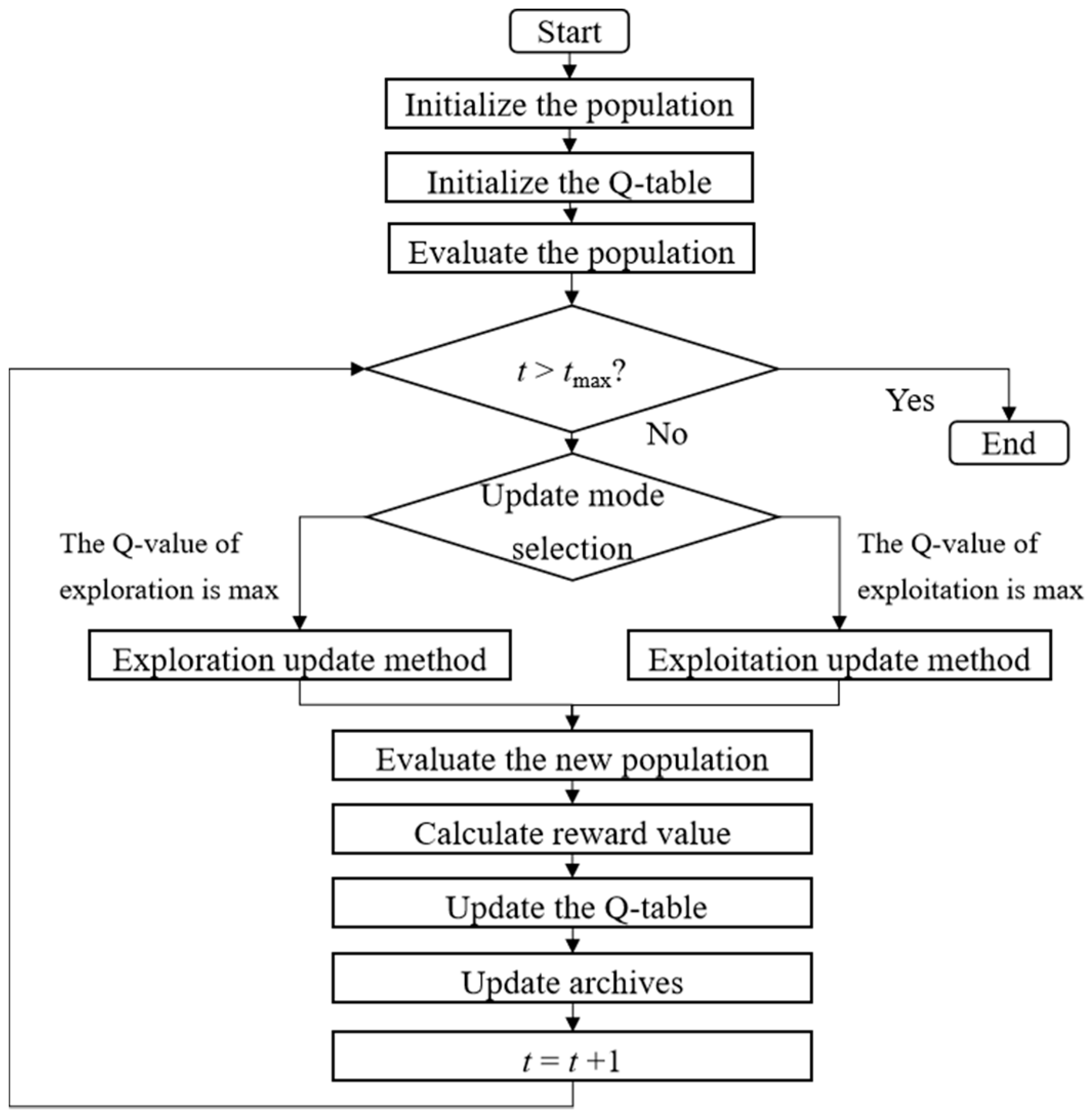
3.4. Framework of GMOPSO-QL

In summary, the framework of GMOPSO-QL is shown in Figure 2.

3.5. Computing Complexity

The main calculation of GMOPSO-QL is in the iterative optimization process. Assume that N is the number of individuals in the particle population, M is the number of objective functions, and t_max is the maximum number of iterations.

During iteration, each particle selects one of the two update modes according to its own state. However, no matter which one is selected, the total time complexity of the particle updating process is O(N). When updating external archives, the time complexity is mainly due to the non-dominated sorting operator. At this point, each particle must be compared with other particles on each objective function, and the time complexity of this process is O(MN²).

Therefore, the time complexity of the proposed algorithm is O(MN²) in each iteration, and the total time complexity of it is O(t_max·MN²), which is the same as the standard MOPSO algorithm. The analysis shows that the improved algorithm does not increase the time complexity and still maintains high execution speed.

4. Path Planning Based on GMOPSO-QL

4.1. Problem Modelling

The representation of the flight path is the basis of UAV path planning [1,28]. In the three-dimensional (3D) flight space, the UAV path can be described by a set of discrete waypoints {p₀, p₁, p₂,…, p_N, p_N+1} and the coordinate of p_k is (x_k, y_k, z_k), where the first waypoint p₀ is the start point and the last waypoint p_N+1 is the target point. This method can represent any flight path in 3D space. The Bezier curve is usually used to ensure the smoothness of the UAV flight path [18,28], since it can describe a better path with fewer control points. In this paper, the cubic B-spline curve is employed to represent the flight path of UAV.

Evaluation objectives (fitness functions) of a UAV flight path contain the flight cost and performance constraints. The following multi-objective optimization model can be established to describe the constrained path planning problem:

$$\begin{array}{l}\min \mathit{f}=\mathbf{\left(}J,C\mathbf{\right)}\\ \mathrm{with}\\ J=J_{\mathrm{L}}+J_{\mathrm{H}}\\ C=C_1+C_2+C_3+C_4\end{array}$$

(8)

where J is the flight cost including length cost J_L and flight altitude cost J_H; C is the sum of constraint costs including threat constraint C₁, terrain constraint C₂, turning constraint C₃, and climbing and gliding constraint C₄. Both the cost functions and the constraints are described as follows.

(1) J_L denotes the flight length cost, which can be calculated as follows [28]:

$$\begin{array}{l}{J}_{\mathrm{L}}={\displaystyle \mathbf{\sum }_{k=0}^N{l}_k}\\ \mathrm{with}\\ l_k=\sqrt{{\mathbf{\left(}{x}_{k+1}-x_k\mathbf{\right)}}^2+{\mathbf{\left(}{y}_{k+1}-y_k\mathbf{\right)}}^2+{\mathbf{\left(}{z}_{k+1}-z_k\mathbf{\right)}}^2}\end{array}$$

(9)

(2) J_H denotes the flight altitude cost ensuring the low-flying benefits, calculated as follows [28]:

$$\begin{array}{l}{J}_{\mathrm{H}}={\displaystyle {\mathbf{\int }}_{Path}{H}_p\mathrm{d}l}\\ \mathrm{with}\\ H_p=\left\{\begin{array}{l}0\hspace{1em}\mathrm{if}\hspace{1em}{z}_k<0\hfill \\ z_p\hspace{1em}\mathrm{otherwise}\hspace{1em}\hfill \end{array}\right. \end{array}$$

(10)

where z_p is the height of the waypoint p.

(3) The threat constraint function C₁ is the sum of all detection probabilities and killing probabilities, which is calculated as follows [5]:

$$\begin{array}{l}{C}_1={\displaystyle \mathbf{\sum }_{k=1}^N\mathbf{\left(}{P}_{R,k}+P_{M,k}+P_{G,k}\mathbf{\right)}}\\ \mathrm{with}\\ P_{R,k}=\left\{\begin{array}{cc}0& d>R_{\mathrm{R}\max }\\ \frac{R_{\mathrm{R}\max }^4}{d^4+R_{\mathrm{R}\max }^4}& d\le R_{\mathrm{R}\max }\end{array}\right.\\ P_{M,k}=\left\{\begin{array}{cc}0& d>R_{\mathrm{M}\max }\\ \frac{R_{\mathrm{M}\max }^4}{d^4+R_{\mathrm{M}\max }^4}& d\le R_{\mathrm{M}\max }\end{array}\right.\\ P_{G,k}=\left\{\begin{array}{cc}0& d>R_{\mathrm{G}\max }\\ \frac{R_{\mathrm{G}\max }}{d+R_{\mathrm{G}\max }}& d\le R_{\mathrm{G}\max }\end{array}\right.\end{array}$$

(11)

where d is the distance from UAV to the threat center; P_R is the radar detection probability, P_M is the killing probability of ground-to-air missiles, P_G is the killing probability of anti-aircraft gun; R_{R max} is the radar’s detection radius, and R_{M max} and R_{G max} are the maximum hit radiuses of the missile and the anti-aircraft gun.

(4) The terrain constraint function C₂ makes the UAV fly higher than the predetermined safe flight altitude, which is expressed as follows [5]:

$$\begin{array}{l}{C}_2={\displaystyle \mathbf{\sum }_{k=1}^N{q}_k}\\ \mathrm{with}\\ q_k=\left\{\begin{array}{l}1\hspace{1em}\mathrm{if}\hspace{1em}{H}_{\mathrm{safe}}<z_k-H_{\mathrm{surf}}\mathbf{\left(}{x}_k,y_k\mathbf{\right)}\hfill \\ 0\hspace{1em}\mathrm{otherwise}\hspace{1em}\hfill \end{array}\right.\end{array}$$

(12)

where H_safe is the minimal safe flight height, and H_surf(x_k, y_k) is the ground level at the position (x_k, y_k).

(5) The turning angle constraint function C₃ is introduced to constrain the UAV’s flight on the plane to obtain a smoother path, which is expressed by [18]:

$$\begin{array}{l}{C}_3={\displaystyle \mathbf{\sum }_{k=1}^N{q}_k}\\ \mathrm{with}\\ q_k=\left\{\begin{array}{l}1\hspace{1em}\mathrm{if}\hspace{1em} {\phi }_k>{\phi }_k^{\max }\hfill \\ 0\hspace{1em}\mathrm{otherwise}\hspace{1em}\hfill \end{array}\right.\end{array}$$

(13)

where φ_k represents the trajectory turning angle at the waypoint p_k. The maximum turning angle φ_k^max can be expressed as

$${\phi }_k^{\max }=\frac{n_{\max }g}{V}\cdot \sqrt{{\mathbf{\left(}{x}_{k+1}-x_k\mathbf{\right)}}^2+{\mathbf{\left(}{y}_{k+1}-y_k\mathbf{\right)}}^2}$$

(14)

where n_max denotes the maximum lateral overload, g is the acceleration of gravity, and V denotes the flight velocity.

(6) The UAV slope s_k at the waypoint p_k needs to meet certain restrictions, which constrains the UAV’s flight in the vertical direction. The climbing and gliding slope constraint function C₄ is calculated as follows [5]:

$$\begin{array}{l}{C}_4={\displaystyle \mathbf{\sum }_{k=1}^N{q}_k}\\ \mathrm{with}\\ q_k=\left\{\begin{array}{l}1\hspace{1em}\mathrm{if}\hspace{1em}{s}_k\ge {\alpha }_k \left|\right| s_k\le {\beta }_k\hfill \\ 0\hspace{1em}\mathrm{otherwise}\hspace{1em}\hfill \end{array}\right.\\ s_k=\frac{z_{k+1}-z_k}{\sqrt{{\mathbf{(}{x}_{k+1}-x_k\mathbf{)}}^2+{\mathbf{\left(}{y}_{k+1}-y_k\mathbf{\right)}}^2}}\end{array}$$

(15)

where α_k and β_k denote the maximum climbing and gliding slopes as follows:

$$\begin{array}{l}{\alpha }_k=-1.5377\times {10}^{-10}{z}_k^2-2.6997\times {10}^{-5}{z}_k+0.4211\\ {\beta }_k=2.5063\times {10}^{-9}{z}_k^2-6.3014\times {10}^{-6}{z}_k-0.3257\end{array}$$

(16)

4.2. GMOPSO-QL for Path Planning

The application of GMOPSO-QL to the UAV path planning problem under 3D complex environments can be implemented according to the framework shown in Algorithm 3.

Algorithm 3. GMOPSO-QL based path planning
	/*Input for GMOPSO-QL*/
	Set maximum iteration number tmax, the number of control points n and parameters λinitial, λfinal, ω, γ.
	/*Initialization*/
	Set the generation number t = 1.
	Set the initial Q-table: Q(s,a) = 0.
	Initialize the location xi and velocities vi of particles randomly, i = 1,2,...,NP.
	/*Evaluation*/
	Generate the smooth trajectory Path = {p0, p1, p2, …, pN, pN + 1}.
	Evaluate flight path performance indicators by Equation (8).
	/*Establish archives*/
	Non-dominated sorting and save non-dominated solutions to archives A.
	/*Iteration computation*/
	while t < tmax do
		Calculate the learning rate λ by Equation (6).
		for each particle i do
			Choose the best a for the current s from Q-table.
			switch action
				case 1: Exploration update mode
					Update the velocity vi and position xi by Equations (2) and (4) with c11 = 1.5 and c21 = 0.4.
				case 2: Exploitation update mode
					Update the velocity vi and position xi by Equations (2) and (5) with c12 = 0.4 and c22 = 1.5.
			end switch
			for each dimension j do
				if the velocity vi or position xi out of bounds, then limit them by $v_{ij}=\left\{\begin{array}{c}{v}_{\max }\hspace{1em}if\hspace{1em}v>v_{\max }\\ v_{\min }\hspace{1em}if\hspace{1em}v<v_{\min }\end{array}\right.$ and $x_{ij}=\left\{\begin{array}{c}{x}_{\max }\hspace{1em}if\hspace{1em}x>x_{\max }\\ x_{\min }\hspace{1em}if\hspace{1em}x<x_{\min }\end{array}\right.$
			end for
			Update the personal best position xpbest,i.
			Calculate the reward r by Equation (7).
		end for
		Update the Q-table by Equation (3).
		Update the archives A
		t = t +1.
	end while
	/*Output*/
	Output the best path for UAV.

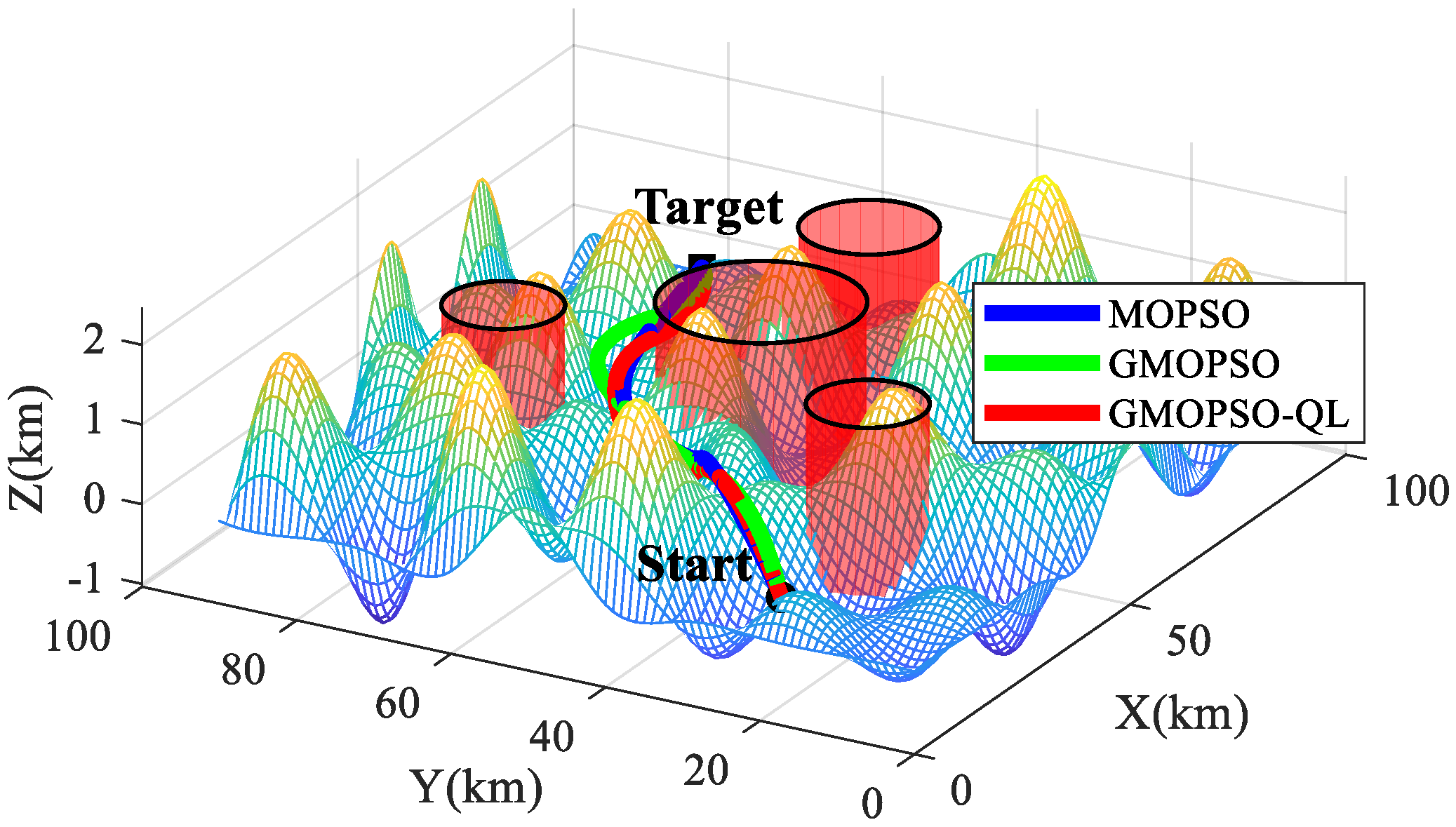
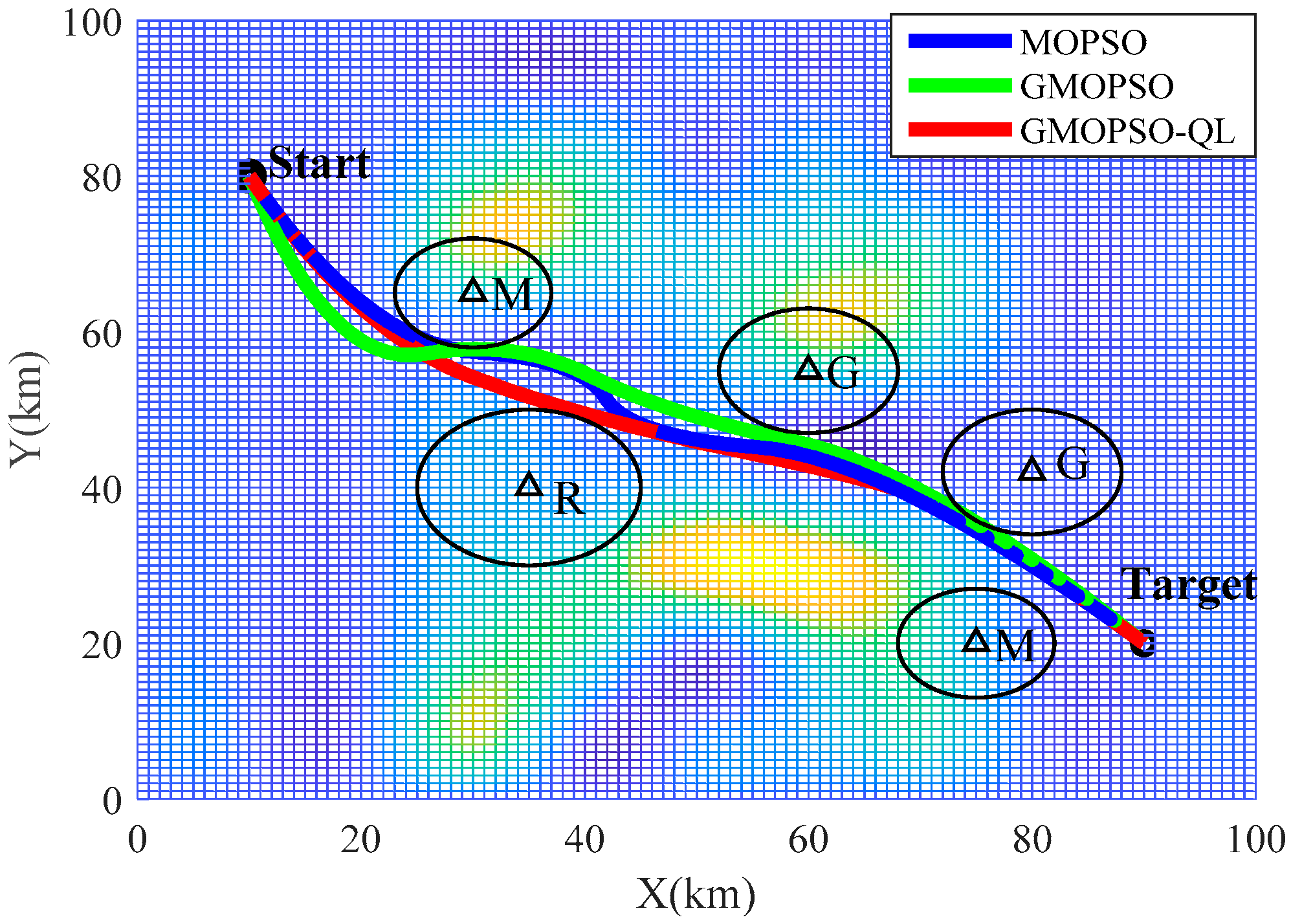
5. Simulation Results

In this section, numerical simulations are performed on the test cases to test the effectiveness of our proposed GMOPSO-QL in solving the constrained path planning problem. The experimental platform used was Intel(R) Core(TM) i5, 2.30 GHz CPU, 16 GB memory, and Windows 10. Matlab-R2018a was used to perform simulation experiments. We simulated the mission scenarios similar to valleys and mountainous environments, with L_max = 100 km long and W_max = 100 km wide. Several threats are set in the scene, and their center and radius are known. To ensure that the calculated constraint costs are as consistent as possible with the actual situation, we set the UAV’s parameters in the simulation experiments according to some real physical parameters and relevant reference [5]: the maximum flying altitude is H_max = 4 km, the maximum lateral overload is n_max = 5, the minimum safe flying altitude is H_safe = 50 m, and the constant flying speed is V = 200 m/s.

We compare our proposed GMOPSO-QL algorithm with the basic GMOPSO [29] and MOPSO [30] algorithms. To ensure the comparability of the three algorithms, the same fitness evaluation method is adopted, and the initial particles are generated by random initialization. Each algorithm is performed 50 times for path planning independently. The main parameters of GMOPSO-QL include the maximum iteration number t_max = 400, the population size NP = 50, the initial and final learning rates λ_initial = 0.9, λ_final = 0.1, the inertia weight ω = 0.4, the discount factor γ = 0.5. Set the number of control points n = 4, that is, D = 3n = 12 parameters need to be determined to generate a smooth UAV flight path. The relevant parameters of GMOPSO and MOPSO are set according to the references [29,30].

Figure 3 displays the plane view of the best paths generated by the three algorithms in 50 runs in Case 1. Figure 4 shows the best flight paths in the 3D environment. The black circle covers the threat area. The labels R, M, and G represent radars, missiles, and anti-aircraft guns, respectively. The vertical profiles corresponding to the best paths in Figure 4 are displayed in Figure 5. It can be seen that all three algorithms can avoid threats and obtain a safe path that meets performance constraints. However, compared with GMOPSO and MOPSO, the best path obtained by the GMOPSO-QL algorithm is smoother and better. From the perspective of the vertical profiles of the best paths, the path planned by the GMOPSO-QL algorithm is gentle and can maintain low-altitude flight. Intuitively, the proposed algorithm can converge to a better solution. Compared with GMOPSO and MOPSO, it has good convergence.

Pareto frontiers of the 50 runs are operated by the Pareto sorting scheme. The finally obtained Pareto frontier is shown in Figure 6. It can be seen that all three algorithms can get a complete Pareto frontier. The Pareto solution set obtained by GMOPSO-QL is closer to the coordinate axis, which indicates that the objective function values obtained by the proposed algorithm is smaller, and its Pareto frontier is superior to the other two comparison algorithms. The proposed algorithm shows the most satisfactory performance.

Table 1. Comparison results of various algorithms in Case 1.

	Best	Median	Mean	Worst	Std.	FR(%)	AT (s)
MOPSO	137.22	169.16	176.38	293.92	34.13	70	69.38
GMOPSO	151.80	194.68	215.12	399.84	50.53	96	70.54
GMOPSO-QL	126.78	160.74	172.22	350.96	44.85	100	69.40

lists the statistical data during 50 runs, including the best, median, mean, and worst values, as well as the standard deviation of the path cost, where the best data in the three algorithms are marked in bold. FR represents the ratio of the feasible paths that satisfy the constraints of all 50 runs. AT represents the average time for the algorithm to run once. Note that the statistics listed in columns 2–6 only calculate the successful operation of generating a safe path. Figure 7 is the boxplot corresponding to the statistical results in Table 1.

From Table 1, it can be seen that the overall performance of the GMOPSO-QL is superior to MOPSO and GMOPSO when the average running time is the same, which proves that our proposed modified strategies to the original algorithm are effective. Although MOPSO’s statistical results in Figure 3 appear to be more concentrated than those of the proposed algorithm, MOPSO’s feasibility rate is only 70%, while the proposed algorithm achieves 100%. In addition, for the key indicators of statistical results, including best value, median value and mean value, the proposed algorithm is the best of the three algorithms.

Figure 8 shows the plane view of the best flight paths planned by the three algorithms in 50 runs on Case 2. Figure 9 shows the corresponding best flight paths in the 3D environment. Vertical profiles of the obtained best UAV paths are displayed in Figure 10, and the Pareto frontiers are shown in Figure 11. In addition,

Table 2. Comparison results of various algorithms in Case 2.

	Best	Median	Mean	Worst	Std.	FR(%)	AT (s)
MOPSO	193.28	218.57	219.65	295.92	19.72	82	55.43
GMOPSO	196.21	214.34	221.02	342.23	24.47	98	58.86
GMOPSO-QL	189.41	206.35	210.09	261.35	14.77	98	55.02

lists the statistical data of the flight cost values. Figure 12 is the boxplot of the statistical results in Case 2.

From Figure 8 we can see that all algorithms can achieve a safe and feasible path that avoids threats. Compared with the flight paths generated by MOPSO and GMOPSO, the path planned by GMOPSO-QL is the smoothest, and it can make better use of the terrain environment by maintaining a low-altitude flight. Additionally, the Pareto frontier of GMOPSO-QL is better than that of MOPSO and GMOPSO. Numerical results show that GMOPSO-QL has the best performance. In Table 2, each item of GMOPSO-QL is superior to MOPSO and GMOPSO, which undoubtedly proves the effectiveness of GMOPSO-QL.

Above all, the GMOPSO-QL algorithm performs better than MOPSO and GMOPSO, and is proved to be effective, efficient, and robust enough to achieve a safe, feasible, and smooth path for UAV.

6. Conclusions

In this paper, a multi-objective optimization approach was employed to solve the constrained UAV path planning problem, and the GMOPSO-QL-based UAV path planning method was proposed. In GMOPSO-QL, the exploration and exploitation update modes are designed to modify the performance of the original MOPSO. The exploration update mode refers more to the historical experience of the particles themselves to enhance the diversity of the population, while the exploitation update mode leads particles to move towards the direction of the optimal particle to achieve rapid converging speed. Based on the Q-Learning strategy, GMOPSO-QL balances the global and local searches by organically combining the two update modes. Numerical results indicate that GMOPSO-QL performs well in solving the constrained path planning problem for UAVs. Compared with MOPSO and GMOPSO, GMOPSO-QL has better convergence and robustness. In the future, we will focus on extending the GMOPSO-QL-based path planner to the multiple UAVs system.

References

- Shi, K.M.; Zhang, X.Y.; Xia, S. Multiple swarm fruit fly optimization algorithm based path planning method for multi-UAVs. Appl. Sci. 2020, 10, 2822. [Google Scholar] [CrossRef] [Green Version]
- Zhao, Y.J.; Zheng, Z.; Liu, Y. Survey on computational-intelligence-based UAV path planning. Knowl.-Based Syst. 2018, 158, 54–64. [Google Scholar] [CrossRef]
- Lin, K.P.; Hung, K.C. An efficient fuzzy weighted average algorithm for the military UAV selecting under group decision-making. Knowl.-Based Syst. 2011, 24, 877–889. [Google Scholar] [CrossRef]
- Qu, C.Z.; Gai, W.D.; Zhang, J.; Zhong, M.Y. A novel hybrid grey wolf optimizer algorithm for unmanned aerial vehicle (UAV) path planning. Knowl.-Based Syst. 2020, 194, 105530. [Google Scholar] [CrossRef]
- Zhang, X.Y.; Duan, H.B. An improved constrained differential evolution algorithm for unmanned aerial vehicle global route planning. Appl. Soft Comput. 2015, 26, 270–284. [Google Scholar] [CrossRef]
- Park, C.; Kee, S.C. Online Local Path Planning on the Campus Environment for Autonomous Driving Considering Road Constraints and Multiple Obstacles. Appl. Sci. 2021, 11, 3909. [Google Scholar] [CrossRef]
- Yu, X.B.; Li, C.L.; Zhou, J.F. A constrained differential evolution algorithm to solve UAV path planning in disaster scenarios. Knowl.-Based Syst. 2020, 204, 106209. [Google Scholar] [CrossRef]
- Liu, Y.; Zhang, X.J.; Zhang, Y.; Guan, X.M. Collision free 4D path planning for multiple UAVs based on spatial refined voting mechanism and PSO approach. Chin. J. Aeronaut. 2019, 32, 1504–1519. [Google Scholar] [CrossRef]
- Maw, A.A.; Tyan, M.; Nguyen, T.A.; Lee, J.W. iADA*-RL: Anytime Graph-Based Path Planning with Deep Reinforcement Learning for an Autonomous UAV. Appl. Sci. 2021, 11, 3948. [Google Scholar] [CrossRef]
- Homaifar, A.; Lai, S.; Qi, X. Constrained optimization via genetic algorithms. Simulation 1994, 62, 242–254. [Google Scholar] [CrossRef]
- Saha, A.; Datta, R.; Deb, K. Hybrid gradient projection based genetic algorithms for constrained optimization. In Proceedings of the 2010 IEEE Congress on Evolutionary Computation, Barcelona, Spain, 18–29 July 2010; pp. 1–8. [Google Scholar]
- Wang, Y.; Cai, Z. Combining multiobjective optimization with differential evolution to solve constrained optimization problems. IEEE Trans. Evol. Comput. 2012, 16, 117–134. [Google Scholar] [CrossRef]
- Zhao, M.; Liu, R.; Li, W.; Liu, H. Multi-objective optimization based differential evolution constrained optimization algorithm. In Proceedings of the 2010 Second WRI Global Congress on Intelligent Systems, Wuhan, China, 16–17 December 2010; pp. 320–326. [Google Scholar]
- Kennedy, J.; Eberhart, R. Particle swarm optimization. In Proceedings of the IEEE International Conference on Neural Networks, Perth, WA, Australia, 27 November–1 December 1995; pp. 1942–1948. [Google Scholar]
- Zhang, D.F.; Duan, H.B. Social-class pigeon-inspired optimization and time stamp segmentation for multi-UAV cooperative path planning. Neurocomputing 2018, 313, 229–246. [Google Scholar] [CrossRef]
- Yang, Y.K.; Liu, J.C.; Tan, S.B.; Liu, Y.C. A multi-objective differential evolution algorithm based on domination and constraint-handling switching. Inform. Sci. 2021, 579, 796–813. [Google Scholar] [CrossRef]
- Ma, Y.N.; Gong, Y.J.; Xiao, C.F.; Gao, Y.; Zhang, J. Path Planning for Autonomous Underwater Vehicles: An Ant Colony Algorithm Incorporating Alarm Pheromone. IEEE Trans. Veh. Technol. 2019, 68, 141–154. [Google Scholar] [CrossRef]
- Zhang, X.Y.; Jia, S.M.; Li, X.Z.; Jian, M. Design of the fruit fly optimization algorithm based path planner for UAV in 3D environments. In Proceedings of the 2017 IEEE International Conference on Mechatronics and Automation, Takamatsu, Japan, 6–9 August 2017; pp. 381–386. [Google Scholar]
- Pham, M.; Zhang, D.; Koh, C.S. Multi-guider and cross-searching approach in multi-objective particle swarm optimization for electromagnetic problems. IEEE Trans. Magn. 2012, 48, 539–542. [Google Scholar] [CrossRef]
- Xu, W.; Wang, W.; He, Q.; Liu, C.; Zhuang, J. An improved multi-objective particle swarm optimization algorithm and its application in vehicle scheduling. In Proceedings of the 2017 Chinese Automation Congress, Jinan, China, 20–22 October 2017; pp. 4230–4235. [Google Scholar]
- Sheikholeslami, F.; Navimipour, N.J. Service allocation in the cloud environments using multi-objective particle swarm optimization algorithm based on crowding distance. Swarm Evol. Comput. 2017, 35, 53–64. [Google Scholar] [CrossRef]
- Wang, B.F.; Li, S.; Guo, J.; Chen, Q.W. Car-like mobile robot path planning in rough terrain using multi-objective particle swarm optimization algorithm. Neurocomputing 2018, 282, 42–51. [Google Scholar] [CrossRef]
- Li, Z.H.; Shi, L.; Yue, C.T.; Shang, Z.G.; Qu, B.Y. Differential evolution based on reinforcement learning with fitness ranking for solving multimodal multiobjective problems. Swarm Evol. Comput. 2019, 49, 234–244. [Google Scholar] [CrossRef]
- Chen, Z.Q.; Qin, B.B.; Sun, M.W.; Sun, Q.L. Q-Learning-based parameters adaptive algorithm for active disturbance rejection control and its application to ship course control. Neurocomputing 2019, 408, 51–63. [Google Scholar] [CrossRef]
- Coello, C.A.; Lechuga, M.S. MOPSO: A proposal for multiple objective particle swarm optimization. In Proceedings of the 2002 Congress on Evolutionary Computation, Honolulu, HI, USA, 12–17 May 2002; pp. 1051–1056. [Google Scholar]
- Coelho, L. Novel Gaussian quantum-behaved particle swarm optimiser applied to electromagnetic design. IET Sci. Meas. Technol. 2007, 1, 290–294. [Google Scholar] [CrossRef]
- Qu, C.Z.; Gai, W.D.; Zhong, M.Y.; Zhang, J. A novel reinforcement learning based grey wolf optimizer algorithm for unmanned aerial vehicles (UAVs) path planning. Appl. Soft Comput. 2020, 89, 106099. [Google Scholar] [CrossRef]
- Zhang, X.Y.; Lu, X.Y.; Jia, S.M.; Li, X.Z. A novel phase angle-encoded fruit fly optimization algorithm with mutation adaptation mechanism applied to UAV path planning. Appl. Soft Comput. 2018, 70, 371–388. [Google Scholar] [CrossRef]
- Coelho, L.; Ayala, H.V.H.; Alotto, P. A multiobjective Gaussian particle swarm approach applied to electromagnetic optimization. IEEE Trans. Magn. 2010, 46, 3289–3292. [Google Scholar] [CrossRef]
- Aguilar, M.E.B.; Coury, D.V.; Reginatto, R.; Monaro, R.M. Multi-objective PSO applied to PI control of DFIG wind turbine under electrical fault conditions. Electr. Power Syst. Res. 2020, 180, 106081. [Google Scholar] [CrossRef]