1. Introduction
Geometric information is fundamental to simulation models, Building Information Modelling (BIM), and digital models, yet steel structures often deviate from design due to fabrication errors, construction tolerances, and applied loads [
1]. Detecting such deformations is crucial for ensuring structural safety and performance across the life cycle. Traditional single-point measurement methods are labour-intensive and inadequate for complex assemblies. In contrast, 3D laser scanning offers precise and efficient acquisition of large-scale geometry, while BIM provides semantic context for segmentation and model updating. Integrating point clouds with BIM enables accurate DTs and improved asset management, though challenges remain with noise and occlusion in point clouds [
2]. Steel structures are widely employed in buildings, industrial facilities, and bridge systems due to their high strength-to-weight ratio, durability, and rapid construction speed [
3]. In the case of steel pedestrian bridges, the reliable identification of the actual geometry of members, connections, and local construction details becomes even more critical, as structural behaviour, safety assessment and maintenance planning strongly depend on it. With recent advances in construction automation, Scan-to-BIM has become a standard approach for monitoring progress [
4], assessing quality, and supporting operation and maintenance [
5]. Constructing as-built BIM models of steel structures requires the generation of accurate 3D models enriched with both geometric and semantic information [
6]. Three-dimensional laser scanning is increasingly adopted for this purpose because of its speed and precision in capturing point clouds. However, efficient and accurate data collection remains challenging. While structural members in conventional buildings (e.g., slabs, beams, and columns) are typically simple in shape and relatively easy to capture [
7], steel structures involve complex elements such as H-beams and hollow sections. These components introduce occlusion and irregular geometry, making high-quality data acquisition difficult and often incomplete. Moreover, the acquisition of highly detailed geometric information for steel pedestrian bridge components can significantly reduce data collection efficiency in Scan-to-BIM workflows [
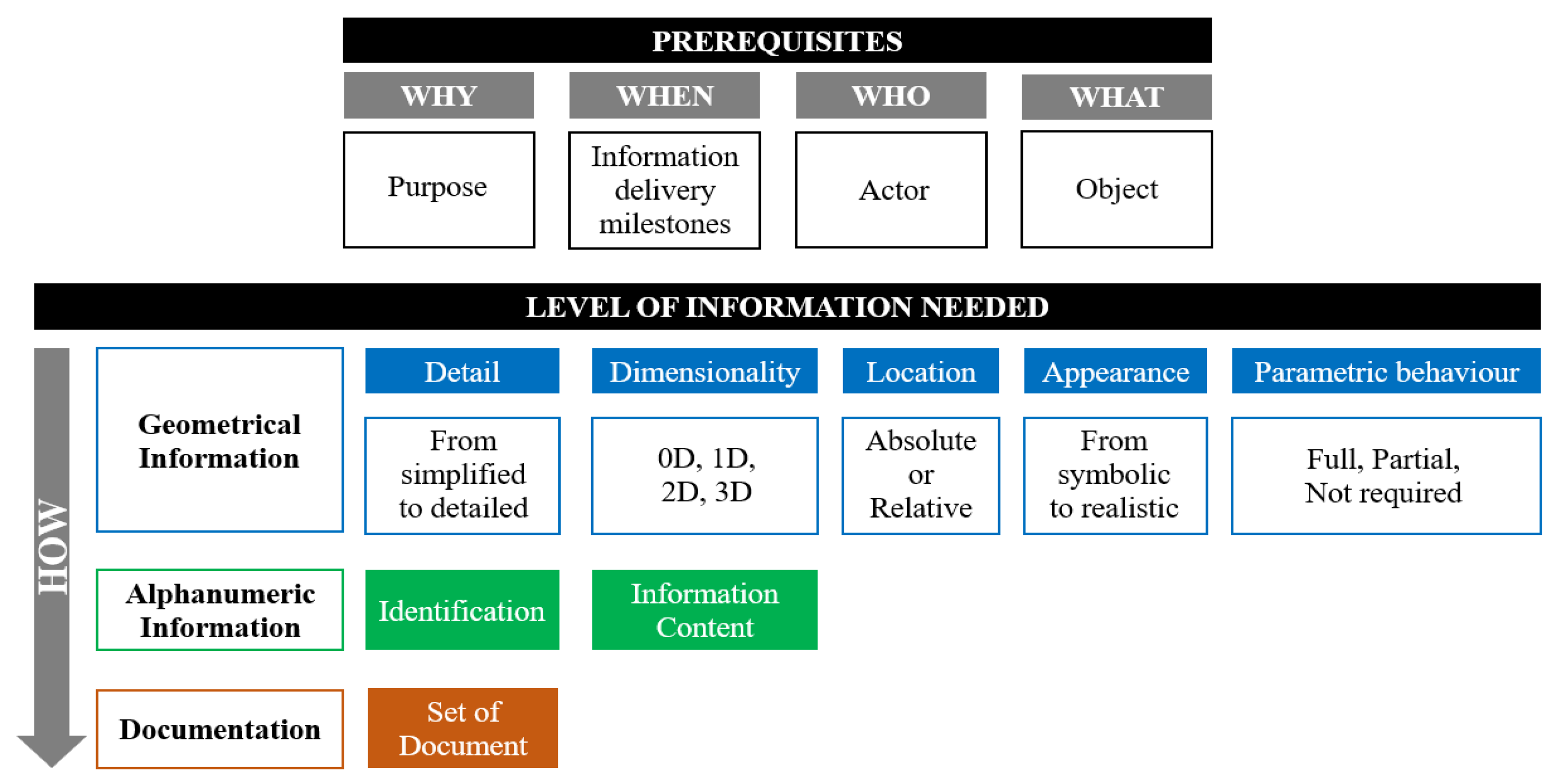
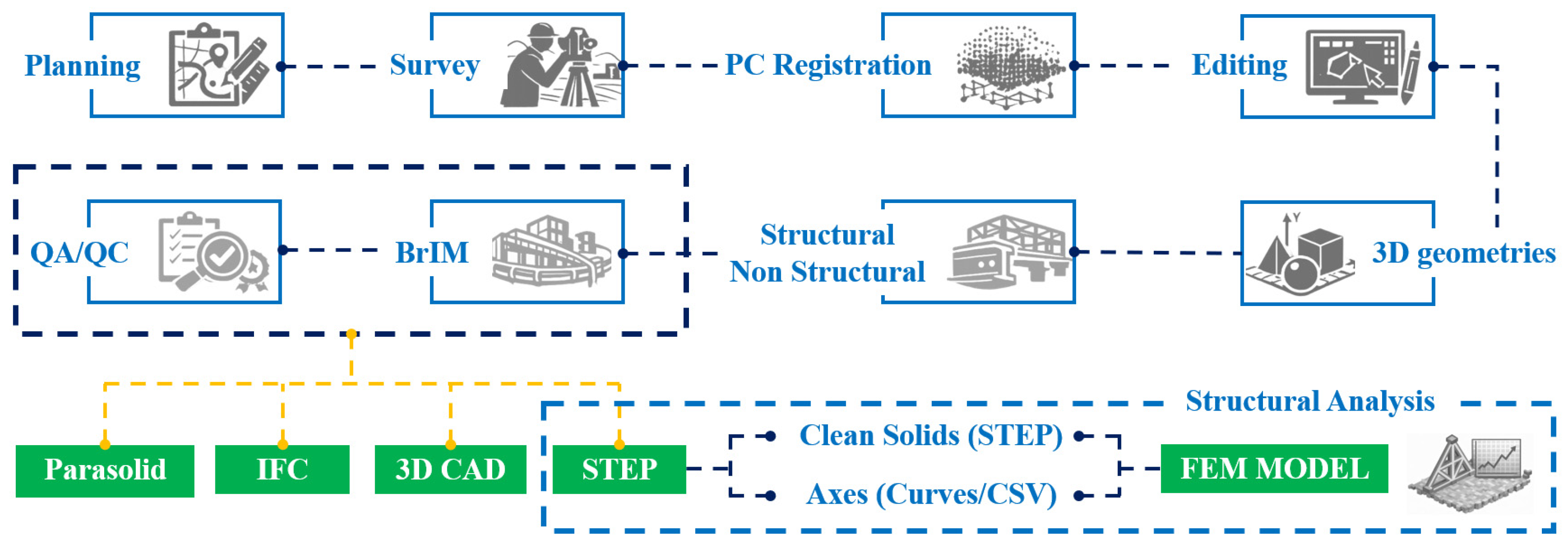
8]. From a Scan-to-BIM perspective, scan planning and data acquisition are therefore primarily driven by geometric requirements, as these directly determine point cloud density, coverage, occlusion handling, and reconstruction fidelity. Within the broader Level of Information Need framework, three complementary types of information are considered: geometrical information, alphanumeric information, and documentation, as shown in
Figure 1.
In
Figure 1, the relationship among the different information types within the Level of Information Need framework was shown. The upper block represents the conceptual definition of information requirements (geometrical, alphanumeric, and documentation), while the lower block illustrates their practical implementation within the Scan-to-BrIM workflow. The arrow labelled “How” indicates the methodological transition from information requirements to data acquisition, processing, and modelling strategies, highlighting how abstract needs are translated into operational procedures.
In the present study, particular attention is devoted to geometrical information, since it directly influences scan planning, point cloud quality, occlusion management, and the achievable fidelity of the final digital model. Nevertheless, alphanumeric attributes (e.g., object IDs, properties, tolerances, and relationships) and related documentation (e.g., specifications, inspection records, and reference drawings) remain essential for validation, traceability, and downstream BIM use; therefore, their explicit definition is strongly recommended in practical Scan-to-BIM projects. Existing scan-planning approaches typically address geometric completeness for individual components or simple steel structures with regular morphology [
9]. However, even within a geometry-focused scope, scan planning for complex steel pedestrian bridge environments remains insufficiently addressed, particularly where varying geometric detail is required across interconnected components. Ensuring adequate geometric data quality, while maintaining alignment with the overall level of information need, is critical for reliable 3D models. With regard to geometric digitisation, Chacón et al. (2021) successfully demonstrated the use of Terrestrial Laser Scanning (TLS) to capture initial imperfections of steel frames and integrate them into BIM-enabled platforms [
8]. Lin et al. (2025) demonstrated that while laser scanning provides accurate geometric information, the management of large-scale point clouds remains labour-intensive and time-consuming [
10]. To address this challenge, they proposed an automated workflow for extracting structural axes from point clouds and updating the corresponding BIM models. Noichl and Borrmann (2025) developed an automated method to reconstruct steel structures from laser-scanned point clouds, addressing challenges of gaps, occlusions, and noise; this approach combines geometric feature analysis with skeleton-based topology preservation, detecting beam instances, refining orientations, and reconstructing missing sections [
11]. However, unlike the present study, their workflow is primarily oriented towards geometric reconstruction and does not explicitly address the integration of the reconstructed model within a complete Scan-to-BrIM-to-FEM pipeline. In contrast, the methodology proposed in this paper emphasises a fully integrated workflow, connecting point cloud acquisition, automated geometric processing, parametric BrIM, and downstream structural analysis. Yang et al. (2020) extracted geometric information of irregular steel components from laser scanning data and automatically generated BIM models [
3]. Similarly, Mirzaei et al. (2022) developed an automatic approach to generate parametric digital models of steel structures from point clouds, extracting geometrical information on member dimensions and cross-sectional shapes using hard-coded knowledge and supervised classification [
2]. Lu et al. (2022) examined the application of 3D laser scanning for steel structure inspection and curtain wall blanking in the Shangqiu Cultural and Art Center; in this latter case study, field comparisons showed that the deviation between the BIM model and the laser-scanned data ranged from 1 to 5 mm, with a root mean square error of 3.5 mm, meeting construction requirements [
12]. Savu et al. (2024) proposed a methodology integrating geodesy, civil engineering, and architecture to improve steel trusses construction management through sustainable practices [
13]. Kim et al. (2024) proposed a deep learning-based Scan-vs-BIM framework for evaluating steel structural integrity by directly comparing As-Built point clouds with As-Planned BIM models [
4]. An extension of the BIM process is called Bridge Information Modelling (BrIM). This process applies digital methodologies to the bridge lifecycle, integrating design, inspection, and maintenance data. For instance, Jeon et al. (2023) developed a BrIM-based maintenance system supporting bridge inspections [
14], while Mohamed et al. (2023) proposed a Scan-to-BrIM workflow for reinforced concrete bridges to optimize structural monitoring and interventions [
15]. While Scan-to-BIM provides the general methodological background, bridge assets require a more specific information modelling framework, namely Bridge Information Modelling (BrIM), due to their distinctive structural configurations, maintenance requirements, and inspection-oriented information needs. In this context, construction details refer to those localised bridge features that are particularly difficult to capture and model reliably, such as stiffeners, gusset plates, bolted and welded connections, secondary attachments, and other non-ideal local configurations whose actual shape may differ significantly from simplified or perfectly symmetrical assumptions. Although such details may appear straightforward to model when assumed to be perfectly shaped, aligned, and symmetrical, their actual condition in existing bridges is often far more complex, making accurate survey and digital reconstruction particularly challenging. In this context, Zhan et al. (2024) developed a semi-automated method for generating IFC-compliant bridge models directly from point clouds, demonstrating how automation can significantly enhance efficiency and accuracy in BrIM creation for maintenance applications [
16]. Complementing these geometry-centric approaches, Crisan et al. (2025) addressed the rehabilitation of heritage steel pedestrian bridges by proposing a BIM-enabled framework focused on the structured definition and implementation of information requirements, including the development of an Information Delivery Specification (IDS) to ensure data consistency, traceability, and quality control throughout the bridge life cycle [
17]. Their work emphasizes the integration of technical inspection data, historical documentation, and structural assessment outputs within a centralized BrIM environment, supporting predictive maintenance, resource optimization, and sustainable rehabilitation planning. In addition, Inzerillo et al. (2025) proposed a workflow for heritage bridges that combines drone-based photogrammetric surveying, AI-powered semantic segmentation of point clouds (using RandLA-Net), and automated generation of parametric BIM models (via AtlasNet, Rhino, and Revit), demonstrating an advanced approach to efficient and accurate BrIM creation for historic structures [
18]. However, limited attention has been paid to scan planning and BrIM generation for steel pedestrian bridges requiring a high degree of geometrical fidelity both at the global scale and at the scale of local construction details. Unlike idealised design representations, real steel pedestrian bridge components often exhibit local deformations, geometric irregularities, fabrication-induced imperfections, and asymmetries that can significantly affect both modelling accuracy and structural interpretation. In this perspective, a high-detail BrIM model derived from point clouds can represent the geometrical and informational backbone of a bridge digital model, supporting future integration with inspection records, monitoring data, and maintenance workflows.
Table 1 compares previous methods in terms of data source, automation level, workflow continuity, semantic modelling capability, and suitability for structural finite element applications.
Recent Scan-to-BrIM research has focused on automating specific tasks such as feature extraction, segmentation, and parametric reconstruction, often using deep learning for geometry detection, BIM updating, or structural inspection. Some approaches also address steel structure reconstruction through advanced segmentation and topology preservation. In contrast, this study proposes an integrated end-to-end workflow that links survey planning, point cloud processing, automated reconstruction, and FEM interoperability. Rather than solving isolated tasks, it ensures a continuous, traceable, and reproducible process from data acquisition to structural analysis, enhancing its practical applicability in engineering contexts.
Despite significant advances in Scan-to-BIM and Scan-to-BrIM methodologies, most existing approaches focus on isolated stages of the workflow, such as segmentation, feature extraction, or parametric reconstruction. While these methods achieve high performance in specific tasks, they often lack continuity between data acquisition, geometric reconstruction, and downstream structural analysis. As a result, current workflows remain fragmented, requiring substantial manual intervention to transform point cloud data into simulation-ready models. This limitation is particularly critical for steel pedestrian bridges, where both global geometry and local construction details must be accurately reconstructed and consistently transferred to FEM environments. In particular, existing Scan-to-BIM approaches do not provide a reproducible and traceable pipeline that ensures the direct transformation of point cloud data into structurally usable models. The absence of such an end-to-end framework limits the applicability of these methods in engineering practice, where interoperability, consistency, and repeatability are essential. Based on these limitations, the research question addressed in this study can be formulated as follows: How can a Scan-to-BrIM workflow be structured to ensure a reproducible, semi-automated, and traceable transformation from point cloud data to simulation-ready structural models, while preserving geometric accuracy and reducing manual intervention?
The main contribution of this study is the definition and validation of a reproducible Scan-to-BrIM pipeline that enables the transformation of point cloud data into simulation-ready structural models. Unlike existing approaches that focus on individual processing steps, the proposed methodology ensures continuity across the entire workflow, from acquisition to FEM interoperability. This contribution is testable through: (i) the geometric accuracy of the reconstructed model, evaluated via point cloud-to-model deviation; (ii) the level of automation achieved in structural element extraction and classification; (iii) the usability of the resulting model within FEM environments without additional manual restructuring.
The aim of this manuscript is to develop a semi-automated Scan-to-BrIM method for generating a high-detail BrIM model of a steel pedestrian structure from point clouds, with particular attention to the reliable reconstruction of both global geometry and difficult-to-capture construction details, as a basis for downstream structural applications. To achieve this aim, the main objectives of the research are: (i) to develop a semi-automated Scan-to-BrIM workflow for high-detail reconstruction of steel structures from point clouds; (ii) to improve the preliminary consistency of geometric reconstruction of complex construction details; (iii) to enable the generation of simulation-ready models suitable for FEM applications. The scientific novelty of this work lies in: (1) the integration of scan planning, automated geometric processing, and parametric modelling into a unified and reproducible workflow; (2) the use of deterministic slicing and clustering strategies for reliable under tested conditions extraction of structural features from complex point clouds; (3) the generation of simulation-ready BrIM models through a structured interoperability pipeline (FreeCAD–STEP–FEM) (version 0.21.2); (4) the introduction of automated procedures for handling complex construction details, such as bolt-based plate perforations, which are typically difficult to manage in conventional Scan-to-BIM approaches.
3. Case Study
3.1. Brief Ddescription of the Site
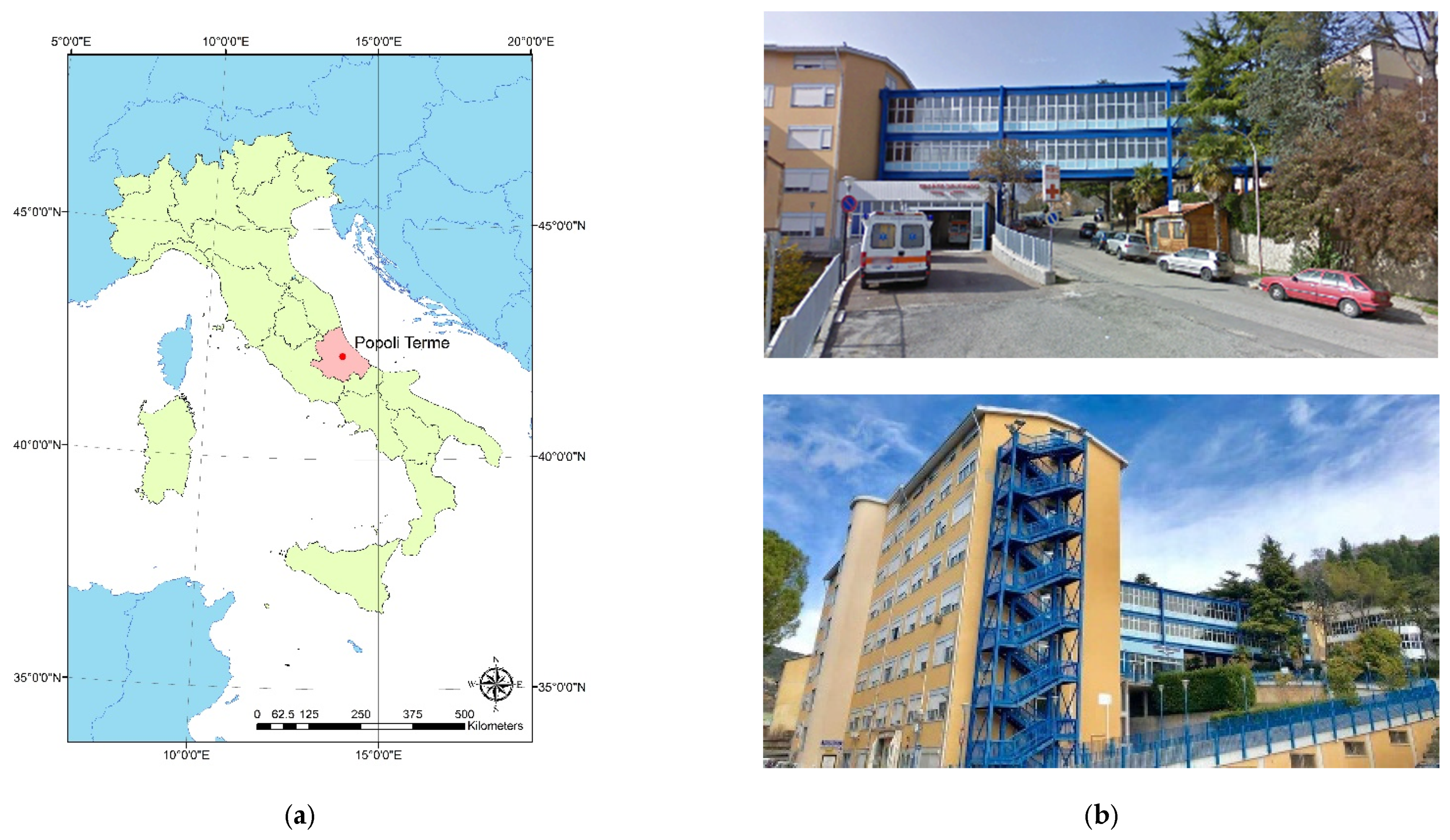
The Popoli Hospital, named after SS. Trinità, is located in the town of Popoli Terme, in the province of Pescara, situated in the central-southern area of Abruzzo (
Figure 4a). The hospital, which has grown over time through successive extensions, consists of several separate buildings, each designed for different clinical and diagnostic functions, but conceived with a view to continuity and integration. From an architectural point of view, the complex is characterised by a rational and functional language, in which regular volumes, linear surfaces and a distribution system organised to ensure maximum efficiency of internal routes prevail.
This is the context for the connecting bridge, an architectural and infrastructural element of primary importance, which links the two main parts of the hospital, crossing over the road below. The analysed structure is a steel pedestrian connection between hospital buildings, functionally and structurally closer to a gallery or enclosed walkway than to conventional bridge typologies. Therefore, the presented methodology is validated on this specific class of structures, and its generalisation to broader bridge categories requires further investigation. The walkway (
Figure 4b), built with a steel supporting structure and completed with glass screens, not only ensures continuity of flow between the wards, but also stands out as a distinctive feature of the entire complex, making the desire to integrate the various hospital functions into a unified system clearly visible from the outside.
From a geometric point of view, the steel pedestrian bridge under consideration is approximately 40 m long, comprises three decks and consists of five braced vertical frames, designated sequentially as A, B, C, D and E. Frame A is the tallest, with a total height of approximately 24 m; the subsequent frames, numbered in order along the length of the structure, are lower in height, measuring approximately 12.65 m for frame B, 13.95 m for frame C and 11.35 m for frames D and E. The typical width of the deck is virtually constant, at approximately 3.32 m.
Table 3 below outlines the dimensions of the main sections of the structural elements.
It should be noted that the present study is based on a single case study, and therefore represents a proof-of-concept validation of the proposed workflow. While the selected structure provides sufficient geometric complexity to test the methodology, further applications to different bridge typologies are required to assess generalisability.
3.2. Three-Dimensional Surveying with TLS
The survey of the bridge connecting the two parts of the Popoli Terme hospital was carried out using a Faro Focus M70 terrestrial laser scanner, an instrument suitable for surveying complex architecture and medium-sized infrastructure, as shown in
Table 4, which lists the main technical characteristics.
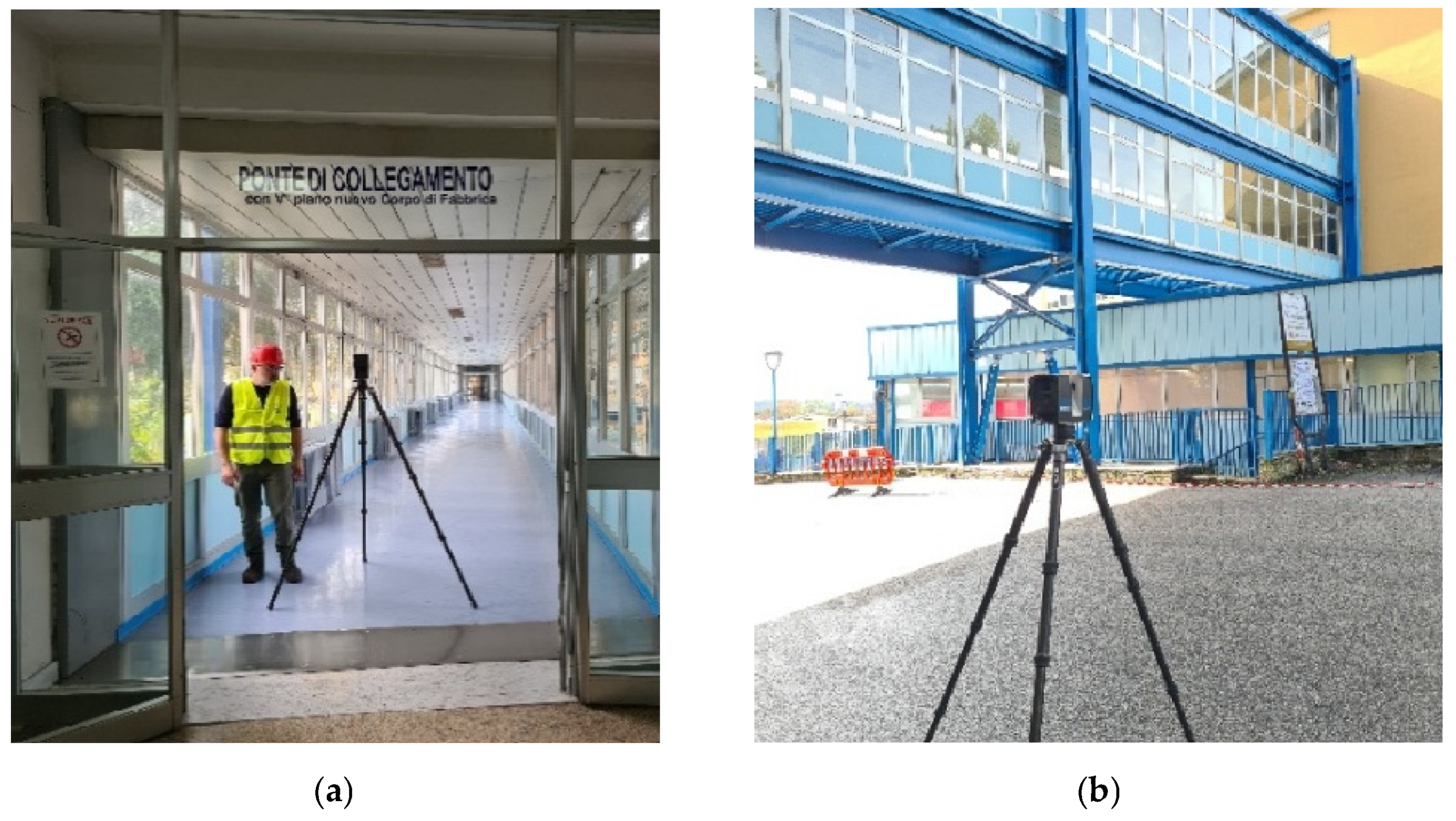
The M70 model operates with a maximum range of approximately 70 m and millimetre-level precision. Combined with its rapid acquisition speed, this allows dense and detailed point clouds to be recorded even in contexts characterised by accessibility constraints or by interference caused by people in transit. In the survey of the Popoli Terme hospital (
Figure 5), a complex scenario was encountered, characterised by driveways that limited the freedom of sensor positioning and by environments, such as the walkways and the emergency room, that required rapid scanning due to the presence of hospital staff and patients. Under these conditions, it was therefore essential to carry out adequate preliminary planning of the survey in order to optimise execution times while ensuring accuracy and preliminary consistency.
The planning phase has been formalised as a deterministic, rule-based procedure, rather than as an implicit process guided by the operator. The workflow follows a structured decision-making framework that can be replicated in similar contexts. In fact, the proposed approach to scan planning is not based on a fully algorithmic optimisation model, but rather on a structured heuristic procedure. This approach represents a practical compromise between fully automated optimisation methods which are often difficult to implement in complex real-world contexts and completely subjective, operator-driven strategies. The survey planning therefore made it possible to identify an acquisition strategy and the correct laser sensor settings in order to combine the hospital’s needs with the survey targets. The quality and resolution were varied according to the distance from the object and the homogeneity of the environments. The differentiated use of parameters made it possible to reduce the overall number of acquisitions and optimise data management, avoiding an excess of unnecessary points in less critical areas.
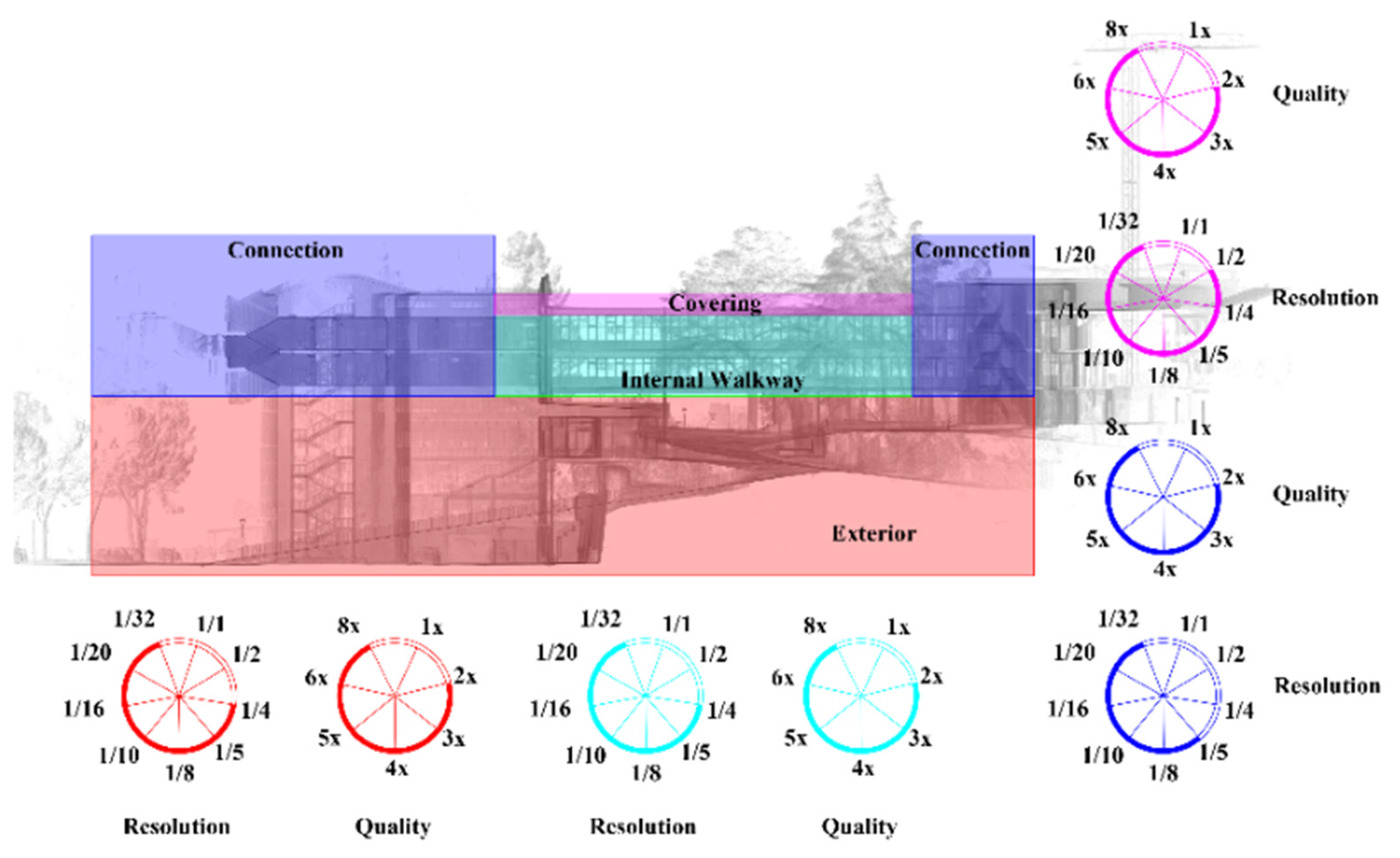
As shown in
Figure 6, four main areas were identified:
external area (95 scans);
connection to internal walkway, corresponding to the access stairs (49 scans);
internal walkways of the bridge arranged on two levels (23 scans);
roof, only partially accessible (6 scans).
Figure 6.
Identifying scan areas with resolution and quality settings diagrams. Colors identify the four scan areas: blue = Connection; pink/magenta = Covering; green/teal = Internal Walkway; red = Exterior. The radar charts use matching colors to show the Resolution and Quality settings applied to each corresponding area.
Figure 6.
Identifying scan areas with resolution and quality settings diagrams. Colors identify the four scan areas: blue = Connection; pink/magenta = Covering; green/teal = Internal Walkway; red = Exterior. The radar charts use matching colors to show the Resolution and Quality settings applied to each corresponding area.
The decision process is supported by preliminary experimental tests, in which different combinations of distance, resolution, and quality parameters were evaluated to assess their impact on point cloud density and feature detectability. These tests provide a reproducible basis for parameter selection, reducing dependence on subjective operator judgement. Once the survey had been planned, to achieve an appropriate level of accuracy during data acquisition, according to the defined rules, it is necessary to identify the correct TLS settings and carefully calibrate the resolution and quality parameters of the point cloud, so as to obtain details such as welds and bolted joints on the beams analysed.
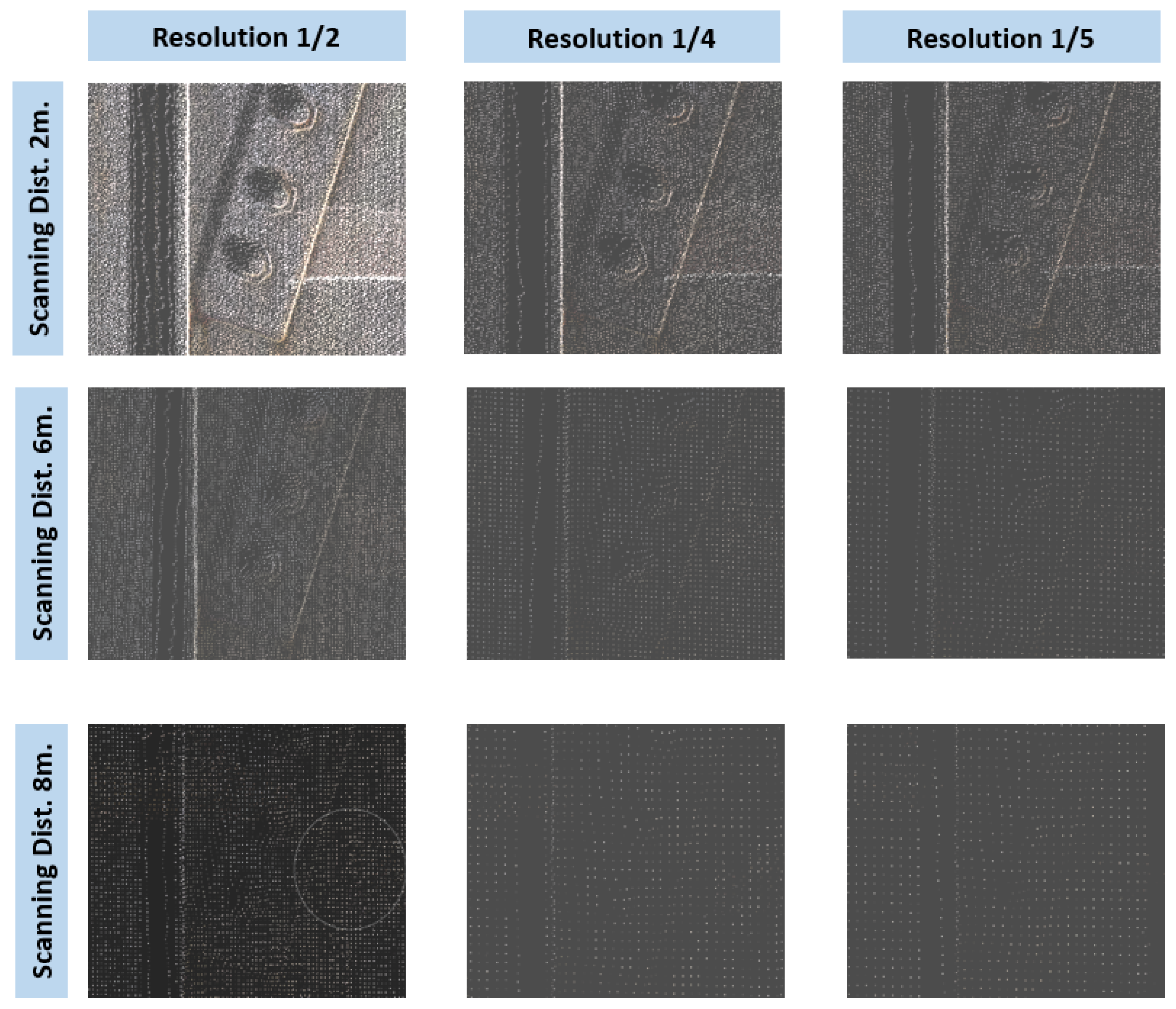
Resolution defines the angular distance between two consecutive points, directly influencing the spacing of the points and therefore the accuracy and precision of the point cloud and the subsequent level of detail; high resolution results in greater point density but also increases scanning times and data storage requirements. At the same time, the quality parameter affects the number of measurements taken for each point detected: high quality values imply the acquisition of more samples per single direction, reducing noise and increasing data preliminary consistency, but with longer operating times. To ensure efficient data collection, several tests were carried out to correctly set the equipment parameters. To ensure consistency, a steel beam with characteristics comparable to those of the surveyed object was selected as a test specimen. Three test scans of this beam were performed, varying only the resolution and quality parameters, as reported in
Figure 7, in order to identify the suitable scanning configuration for accurately capturing a bolted steel beam. The three scanning cycles were repeated at different distances, 2 m, 6 m and 8 m respectively, using the following settings: 1/2 resolution 2X quality, 1/4 resolution 2X quality and 1/5 resolution 2X quality. The scans show that the identification of structural and non-structural elements varies significantly depending on the different setting parameters and the acquisition distance. The proposed Scan-to-BrIM workflow showed good accuracy and efficient processing for the investigated steel bridge. Registration accuracy reached an RMSE of 2.50 mm, while model validation showed a mean deviation of 7.60 mm. The complete workflow required about 7.3 h, including registration, segmentation, BIM, and FEM preparation. The final model contained 146 structural elements, with 78% automatically extracted and only 22% manually refined. These results confirm the effectiveness of the methodology for accurate and FEM-ready bridge digital modelling.
The best results are found in scans performed from 2 m, with a resolution of 1/2 and 2X quality, and 1/4 resolution 2X quality, in which even small elements, such as bolts, can be accurately identified. The disadvantage of this setting (especially for the 1/2 resolution and 2X quality setting) is the long scanning times and increased noise in the acquired data. The least suitable result for identifying small elements is recorded in the scan performed from 8 m, with a setting of 1/5 2X, where the constituent elements are not distinguishable. Analysing the data reported in
Table 5, a significant and consistent decrease can be observed across all resolutions analysed, with losses of around 78–80% between 2 m and 6 m and more than 90% between 2 m and 8 m. This trend demonstrates that distance is a dominant factor in determining the effective resolution of the acquired data, regardless of the instrument’s nominal parameters. This reduction directly affects the level of geometric detail that can be represented in the point cloud, with particularly significant effects on the description of small-scale features.
As regards the ability to recognise details, different acquisition configurations significantly influence the ability to correctly identify small-scale geometric features, such as bolts, plates or connections. Under short-range acquisition conditions, configurations characterised by higher resolution allow for a more complete and legible representation of the geometry, making it possible to reliably recognise even the finest construction details. Conversely, lower-resolution settings tend to reduce the definition of the point cloud, limiting the distinguishability of smaller features and introducing ambiguity in the geometric interpretation. These effects are directly reflected in the overall robustness of the Scan-to-BrIM workflow. A point cloud characterised by high density and low noise levels ensures greater stability during automated processing stages, such as clustering, axis estimation and section reconstruction, improving the consistency and repeatability of results. Conversely, less dense, and noisier datasets can compromise the preliminary consistency of recognition procedures, increasing the risk of errors in the classification of structural elements and the definition of parametric geometries. It follows that the quality of the point cloud is not merely a descriptive aspect but constitutes a determining factor for the effectiveness of the entire modelling process, highlighting the need for a conscious balance between acquisition speed and geometric accuracy.
Considering the resolution and quality parameters analysed, and relating them to distance, which directly affects the accuracy and identification of elements, it was decided to perform modular scans based on the homogeneous areas identified, to achieve a good compromise between data accuracy and execution times.
The external scans and those inside the bridge walkways were performed with a resolution of 1/4 and 2X quality, ensuring a point density suitable for the three-dimensional reconstruction of the construction details. In the connecting areas, consisting of the side access stairs, it was necessary to operate with lower resolutions, partly due to the limitations imposed by the continuous passage of hospital staff. Under these conditions, the scanner was set to acquire scans that required speed of execution, in reflectance mode with 1/5 resolution and 2X quality, reducing the scanning time.
The scans connecting the stairs and the internal walkway of the bridge were essential as there was no visible connection between the interior of the bridge walkway, where there are non-opening windows, and the exterior area. On the other hand, for the scans performed to detect the roof, carried out from the terraces and windows facing the bridge, a higher resolution was adopted, equal to 1/2 resolution and 2X quality, in order to compensate for the greater distance from the bridge and obtain a sufficient point density to accurately describe the upper surfaces and geometries that were not directly accessible.
This approach ensures uniformity between the point clouds and greater detail of the structural elements, simplifying the subsequent registration phases.
Figure 8 shows some of the results obtained from the processing of the point cloud. Particular attention was paid to the scans performed on the two walkways. These scans were particularly noisy due to both the passage of stretchers and medical staff and the point clouds passing through the fixtures, which produced a noisy point cloud. This phase ensured a solid and accurate basis for subsequent processing. The camera active during the recording phases not only enriched the geometric data with realistic colour information, but also generated a navigable virtual tour using Faro scenes software, which is useful for an immersive consultation of the artefact without the need to physically visit the site.
The overall RMSE of the registration process, calculated in FARO SCENE, was found to be 2.50 mm. This value was taken as an indicator of the average geometric error of the registration, representing the internal consistency of the alignment between the different scans. The quality of the registration is further confirmed by the percentage of points with a deviation of less than 4 mm, which stands at 68.9%. The accuracy of the model was assessed by considering both errors associated with the targets and point distance errors from the individual scans. The mean target error was 1.98 mm, with a standard deviation of 2.85 mm and a maximum error of 6.90 mm. Point distance errors generally range between 0.85 mm and 2.98 mm, with a single maximum value of 4.11 mm. Based on these results, the average deviation between the point cloud and the model can be assumed to be approximately 2.2 mm, with an overall model accuracy in the order of 2–3 mm.
After completing the registration process, the entire dataset was exported in E57 format, an open standard that allows both geometric and chromatic information to be retained, ensuring compatibility with various processing software. The file was then imported into PointCab software (Origins 4.2), an environment designed to convert three-dimensional data from the survey into two-dimensional representations traditionally used in technical documentation. Within PointCab, it was possible to generate orthophotos, plans, facades, and profiles directly from the recorded point cloud, setting cutting planes and rasterization parameters consistent with the project requirements. The software allows arbitrary planes to be defined in space and the point cloud to be projected onto them, returning high-resolution images that immediately summarise the three-dimensional complexity of the structure.
3.3. Geometric BrIM of the Existent Steel Structure
The geometric model was developed by importing the point cloud into the Anaconda environment where it was automatically segmented and classified using Python scripts executed through the Spyder IDE. Within this environment, the point cloud was segmented and automatically classified into individual frames by means of Python scripts executed through the Spyder IDE (Integrated Development Environment). This step allowed the development of an automatic workflow for transforming the point cloud of a steel pedestrian bridge into a parametric BrIM model. This workflow aims to overcome the traditional manual modelling and analysis sequence by introducing automation scripts and geometric recognition algorithms in the Rhinoceros-Grasshopper environment, ensuring interoperability and replicability with CAD packages such as FreeCAD (version 0.21.2), BrIM software such as Midas CIM (Version V200), and FEM software such as COMSOL Multiphysics (Version 6.3). Furthermore, starting from a high-resolution point cloud, the process has been made more efficient thanks to preliminary segmentation and classification of structural elements. The proposed deterministic pipeline allows a single vertical frame (composed of two pillars, horizontal beams and braced fields) to be isolated from the high-resolution point cloud acquired on the entire deck. According to the steps described in
Section 2.3, the filtered points are then used to estimate the global longitudinal axis of the bridge using extended PCA in order to ensure robustness with respect to non-uniform densities, typical of LiDAR (or photogrammetric) scans considering the point cloud:
with centre of gravity defined by:
it is possible to construct the covariance matrix:
by calculating the eigenvalues and eigenvectors:
the vector associated with the maximum variance is assumed as the longitudinal direction:
The entire scene is then aligned to orient the cloud along
, making the subsequent section-by-section analysis consistent. After estimating the longitudinal direction
of the bridge and aligning the point cloud accordingly, the workflow described in
Section 2.3 was applied. For each slice, the resulting sections were analysed to identify structural components. The projected points were grouped into clusters, from which simplified geometric representations were derived through robust line fitting, allowing the extraction of dominant segments describing the main structural elements. Finally, once the direction of each segment in the section has been estimated, the features are classified according to their inclination: (i) almost vertical pillars (inclination tolerance
, parallelism
); (ii) horizontal beams (segments with
) and (iii) braces (inclined segments with compatible centre distance and “double C” coupling detected as two parallel lines separated by a constant distance). Scrolling through the sections along
, the features are aggregated into trajectories and checked for continuity. Each longitudinal window (frame candidate) is then given a composite score that combines section flatness (RMS deviation from the cutting plane), verticality and/or parallelism of the pillars, presence of at least one beam, recognition of the double-C brace coupling (modelled as two almost parallel segments at almost constant distance), continuity of the lines between successive sections and density of support points. The maximum score identifies the candidate frame, and geometric refinement is then performed on it, producing as output the stack of orthogonal planes at the frame, the barycentric axes of pillars, beams and braces aligned with the overall system, and clean section polylines consistent with the expected profiles (H/HEA-HEB/HEM, IPE/UPN or double-C). These objects (planes and axes) are used downstream by the Grasshopper workflow to generate sections and parameterise catalogues. The planes connect directly to the Perp Frames/Align Plane nodes to enforce orthogonality, while the axes feed the profile fitting modules, ensuring correct orientation and snap.
Appendix A—Listing A1 (Python script) provides a minimal implementation, executable in Anaconda/Spyder environment with standard libraries (Open3D/NumPy/Scikit-learn), which reproduces the described flow, returning planes and axes ready for import into Rhino/Grasshopper and with thresholds exposed to adapt to different scales and densities.
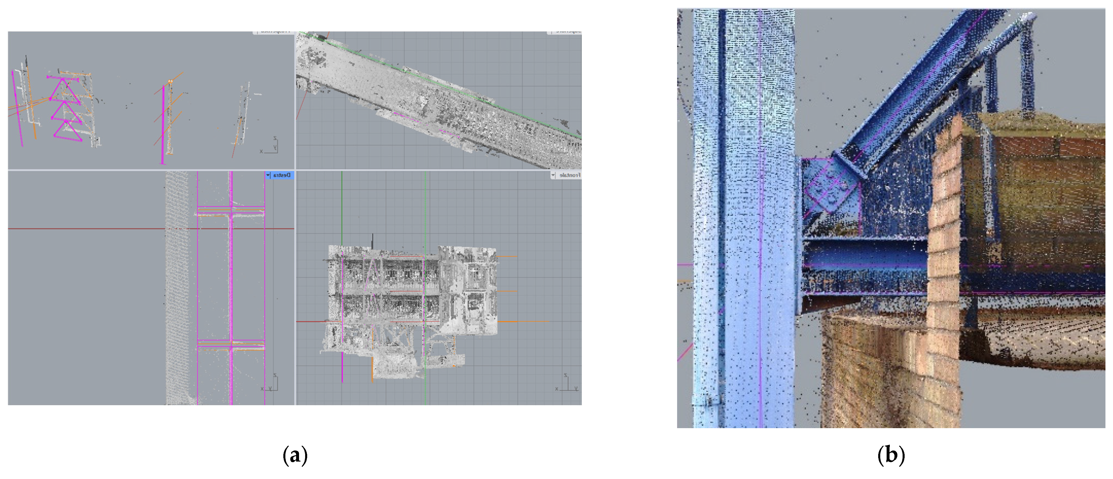
Figure 9a,b show the segmentation of a single frame.
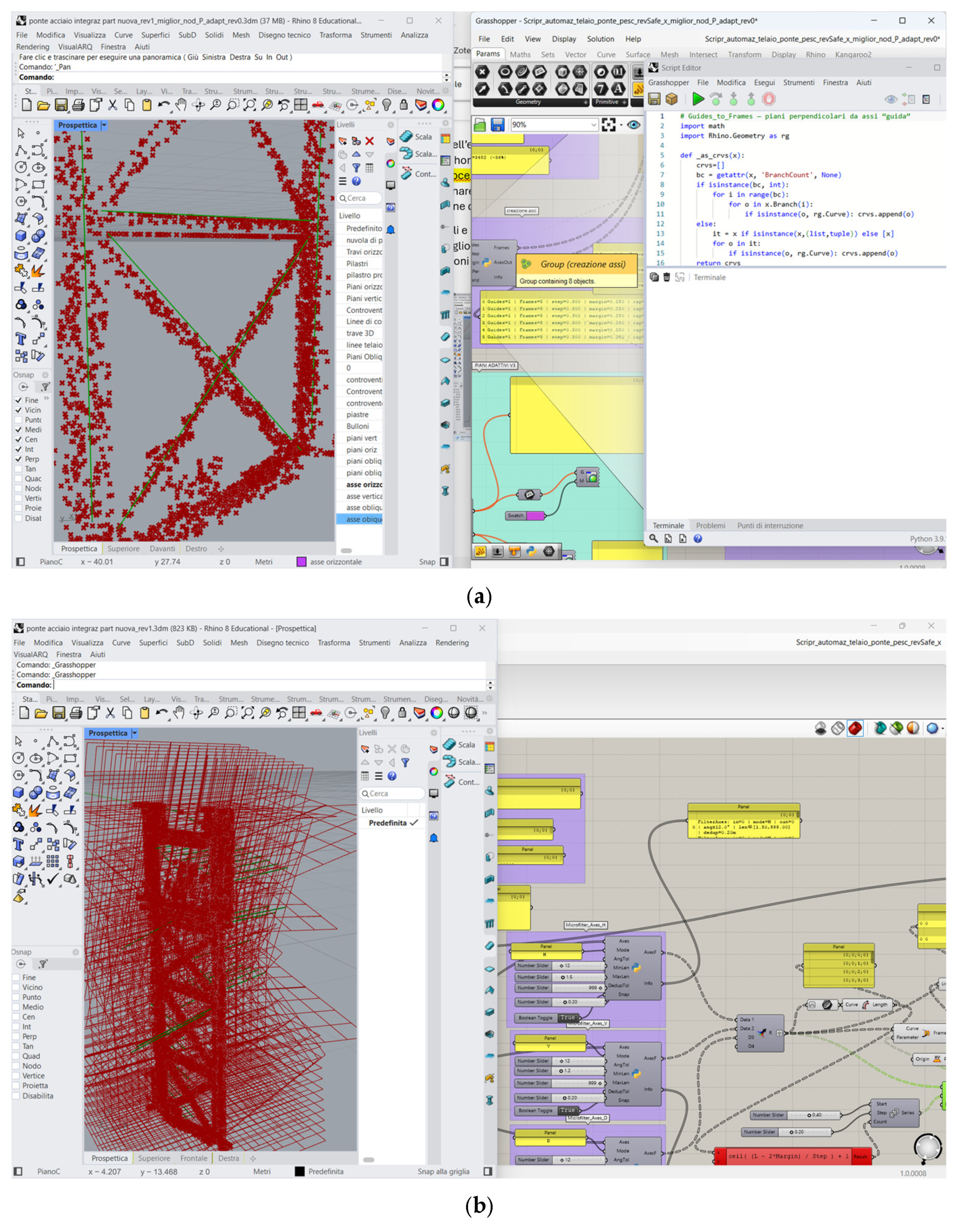
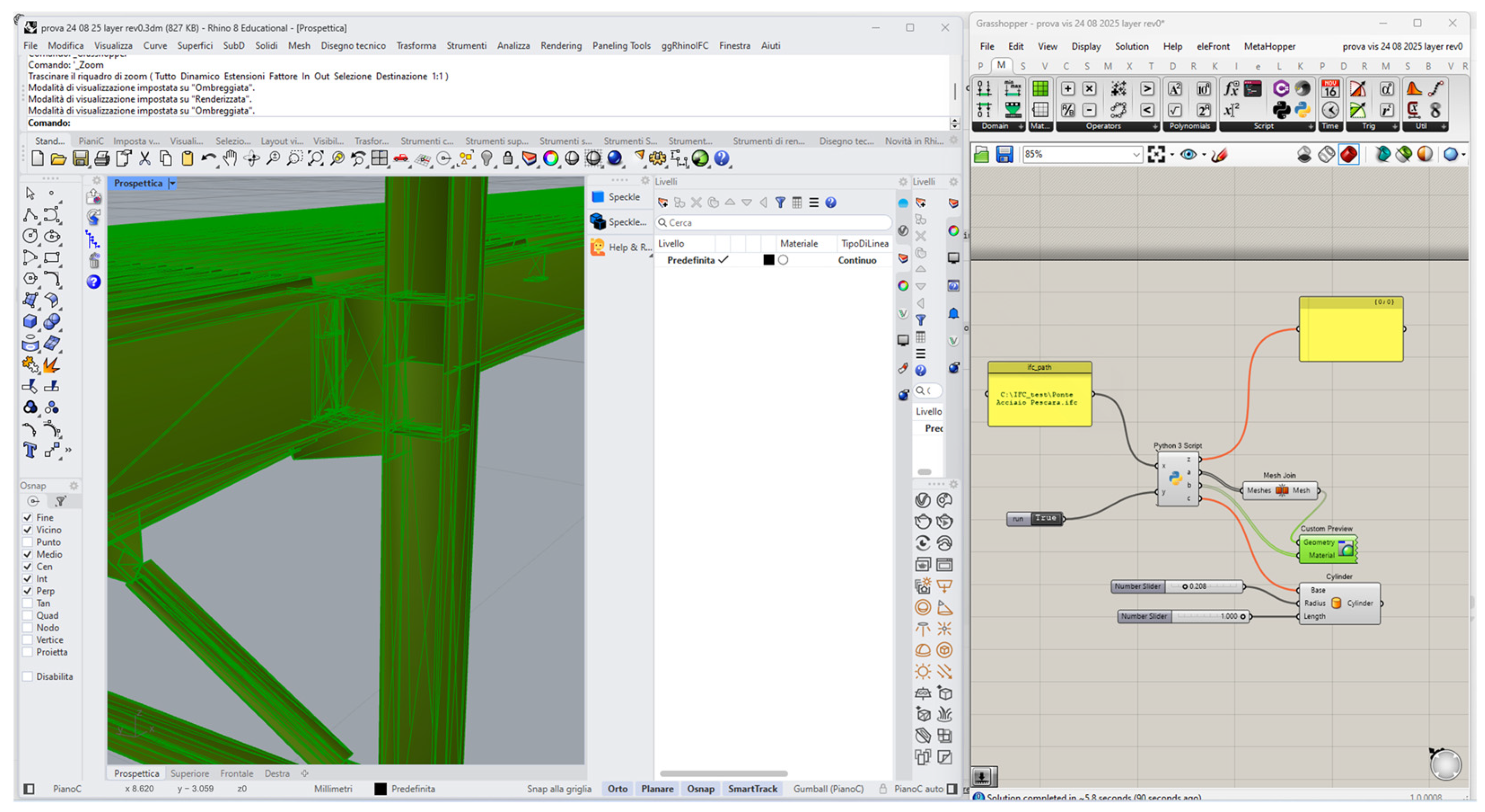
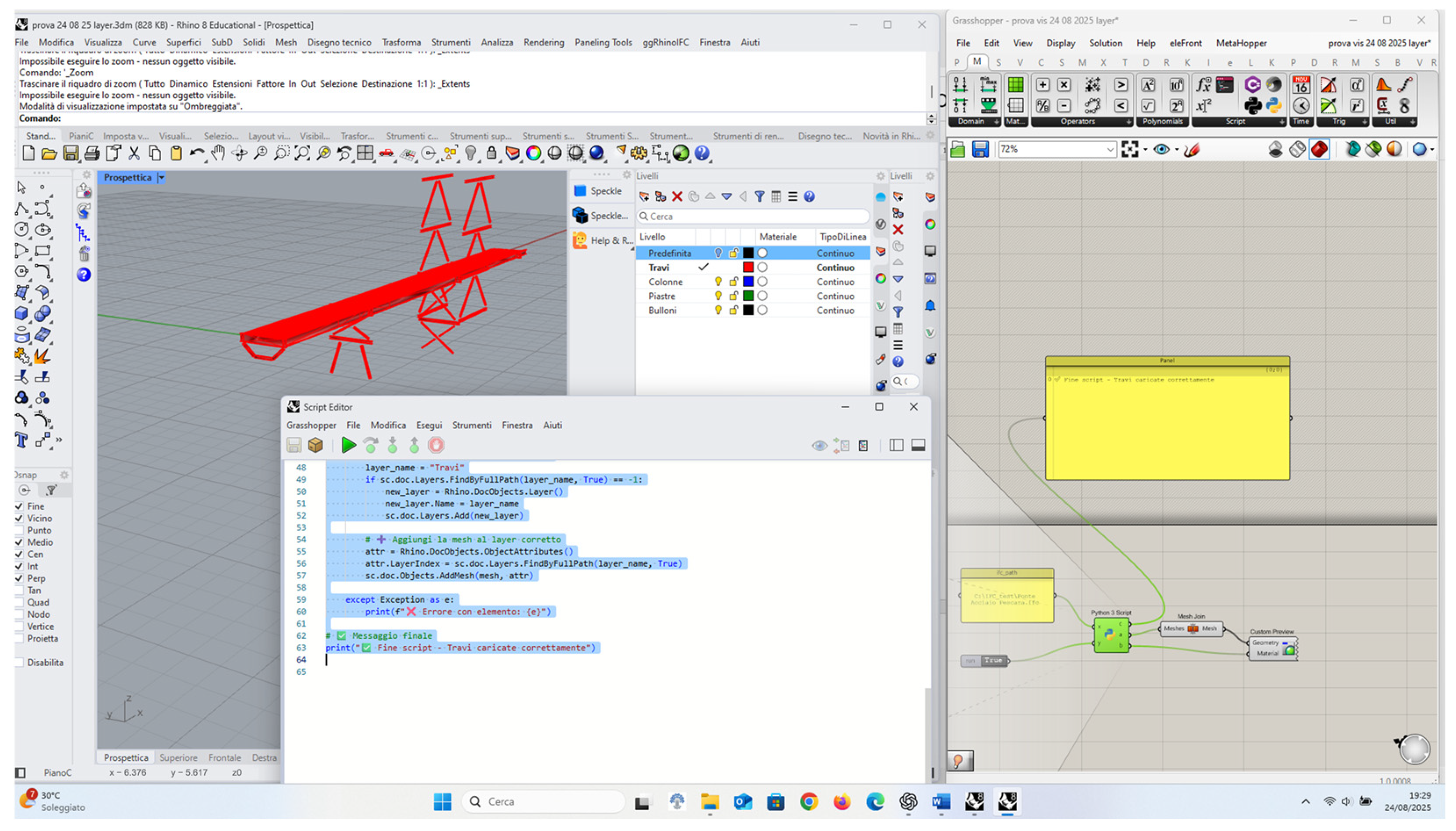
The core of the developed automation consists in processing segmented point clouds within Grasshopper by means of Python scripts. The process starts with the raw point cloud in .e57 or .laz formats, which is imported into Rhinoceros using the Arena4D plugin by Veesus.
Through a preliminary classification system by layer, the cloud is divided into structural categories (individual frames), facilitating the automation of the subsequent processing stages. These scripts recognise the structural elements and extract their main axes. Subsequently, as shown in
Figure 10a,b, a cutting plane perpendicular to each axis is automatically generated, even for inclined elements, allowing regular two-dimensional orthogonal sections to be obtained, avoiding manual errors or geometric inaccuracies.
This approach not only simplifies section extraction, but also ensures greater precision, which is essential for steel models where tolerances are in the order of millimetres. The polylines generated by the sections in the first step are optimised using simplification and smoothing functions based on spatial and angular tolerance to ensure that they faithfully follow the actual contours of the structural elements, without breaks or deviations. To improve stability and repeatability, the flow has been extended with a layered point reducer (Z-Reduce) that preserves vertical uniformity.
To avoid solver crashes and ensure sufficient point density for axis estimation, a robust reducer has been introduced that operates in three modes, automatically selected based on the parameters described below:
if MaxTotal ≥ input points or Keep = 100% is set, the points are not reduced, thus decreasing the computational load.
if a percentage subsample is required, the reducer randomly but reproducibly extracts a set equal to round (Cin·Keep) points where Cin is the total number of input points in the original point cloud.
if a reduction with vertical uniformity is required, the points are divided into bins along the Z axis; a “minimum guaranteed” quota is drawn from each bin and then filled to the total target. This is the key mode for axis estimation.
Table 6 summarised and describe the parameter used for the robust reducer. The expected outputs in this phase consist of the reduced point list with additional diagnostic and debugging information. The reducer is placed upstream of all slow nodes to avoid continuous recalculations while the parameters are being modified, making the entire flow reusable more robust. Once the axes of the structural elements have been identified and validated, the next step is to construct consistent local reference systems, which are necessary for generating sections and for subsequent modelling operations.
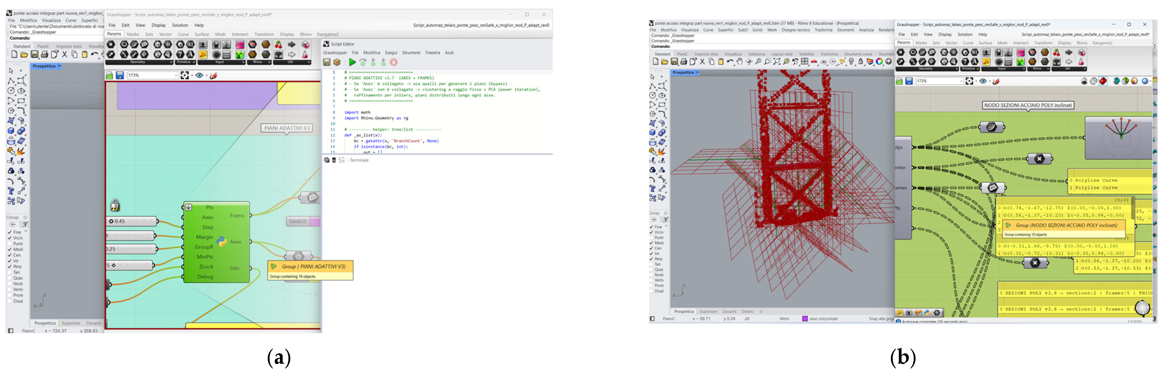
To this end, Adaptive Planes v3 have been introduced, designed to automatically create orthogonal frames aligned with the actual geometry of the elements. Adaptive Planes v3 represent the link between the geometric recognition phase (axis extraction) and the section extraction phase, improving precision and numerical stability to the various real cases found in steel structural models.
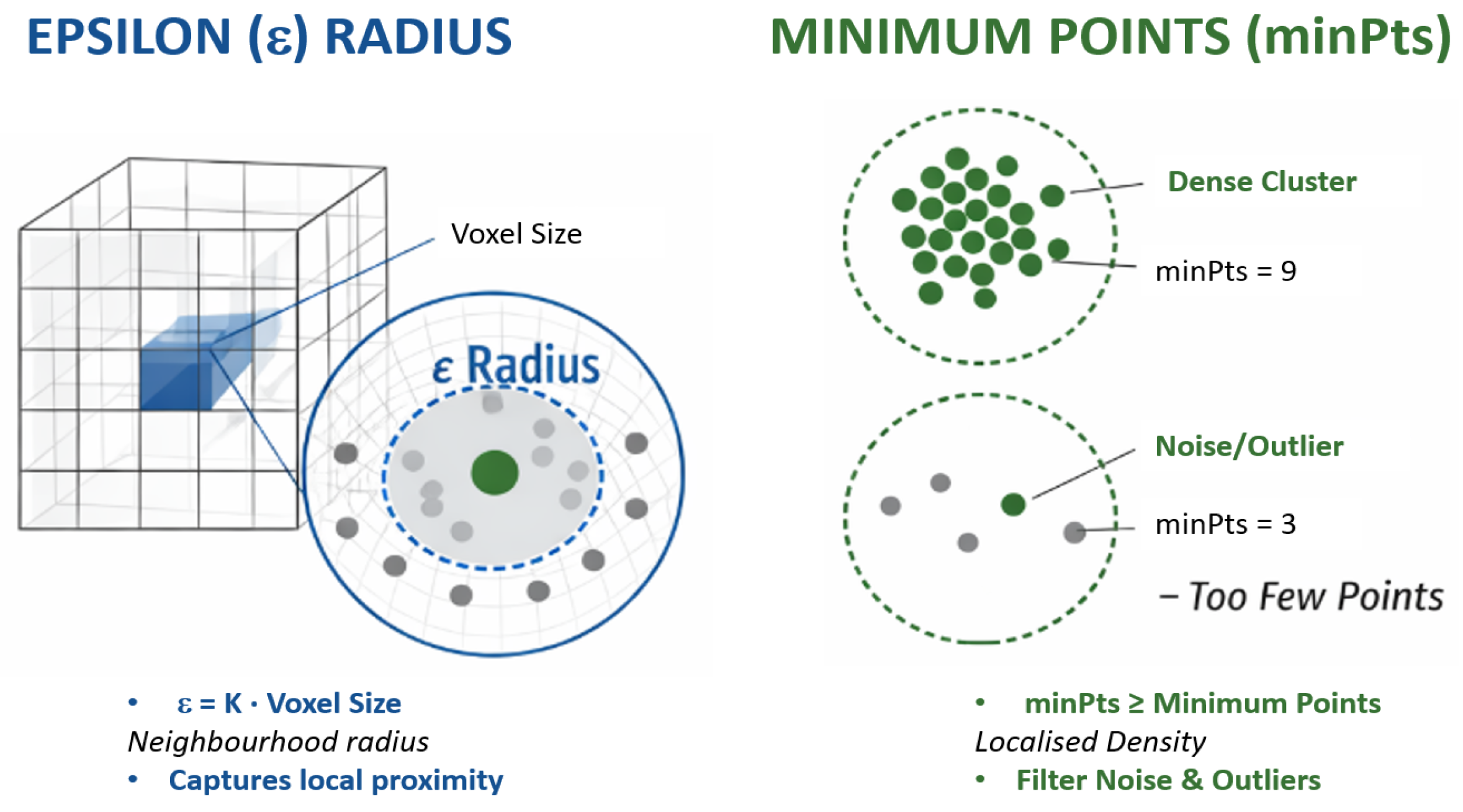
Figure 11 illustrates two prerequisite nodes: the Axes Node, which automatically extracts the structural element axes, and the Adaptive Planes Node, which generates planes perpendicular to those axes. Once the axes are available, Adaptive Planes v3 creates, for each element, a set of local orthogonal frames that serve as the reference for section extraction and subsequent modelling, ensuring consistency and repeatability. The node runs in two modes: BYPASS, when validated axes are provided, generating planes with a specified step and edge margin to cover the element; and Auto fallback, triggered when axes are missing or unreliable, where clustering and PCA/line fitting estimate the axis direction from the point distribution before plane generation. For vertical members (pillars/columns), a Z-Lock option forces alignment with the global direction [0,0,1] when Z is dominant. Key parameters include plane step (typically 0.25–0.40 m), margin, clustering radius (GroupR), minimum points per cluster (MinPts), and Z-Lock (typically enabled for pillars).
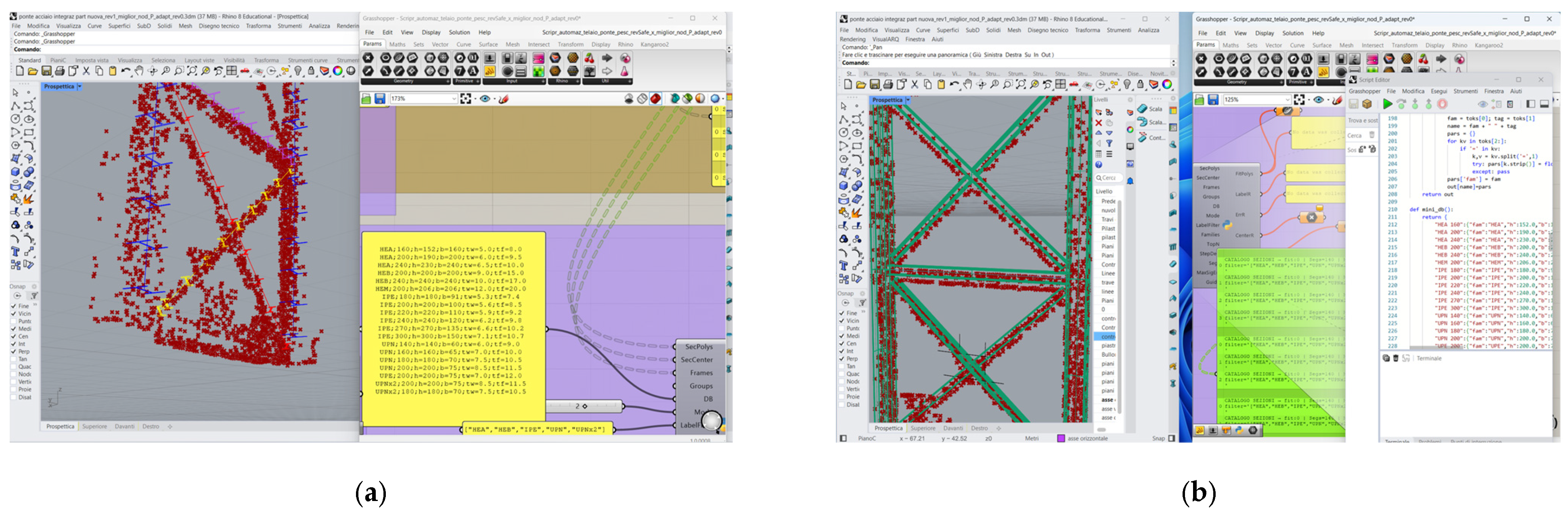
Finally, a Steel Section Catalogue (
Figure 12) matches extracted section polylines to standard profiles; if the fitting error is within threshold, the system returns the section centre, local axes, and family label, enabling automatic structural classification and reducing manual intervention.
A qualitative comparison can be established with traditional manual Scan-to-BIM workflows, where the reconstruction of structural elements is typically performed through manual fitting of sections and axes based on visual interpretation of the point cloud. In such approaches, the modelling process is time-consuming and highly dependent on operator expertise, particularly for complex elements such as bracing systems and connections. In contrast, the proposed workflow automates key stages of the process, including axis detection, section extraction, and structural classification. This reduces manual intervention and improves consistency, particularly in repetitive elements such as beams and frames. While a direct time benchmark was not conducted, the reduction in manual operations represents a significant improvement in workflow efficiency. Compared to existing Scan-to-BIM tools and methodologies, which often focus on specific tasks such as segmentation, feature extraction, or parametric reconstruction, the proposed approach emphasises an end-to-end integration from data acquisition to FEM-ready models. For example, many commercial and research tools require manual intervention for axis definition, section fitting, or model structuring, particularly in the presence of complex steel geometries. The proposed workflow addresses these limitations by introducing a deterministic pipeline for slicing, clustering, and feature extraction, combined with a structured export strategy that ensures interoperability with FEM environments. This allows the generation of simulation-ready models with reduced ambiguity compared to standard BIM outputs.
Table 7 summarises a qualitative comparison between traditional manual modelling, existing Scan-to-BIM approaches, and the proposed workflow. The comparison highlights that the main advantage of the proposed method lies in reproducibility and direct interoperability with FEM environments, rather than in the use of novel algorithms.
3.4. From Parametric Geometry Generation to FEM-Oriented STEP Interoperability
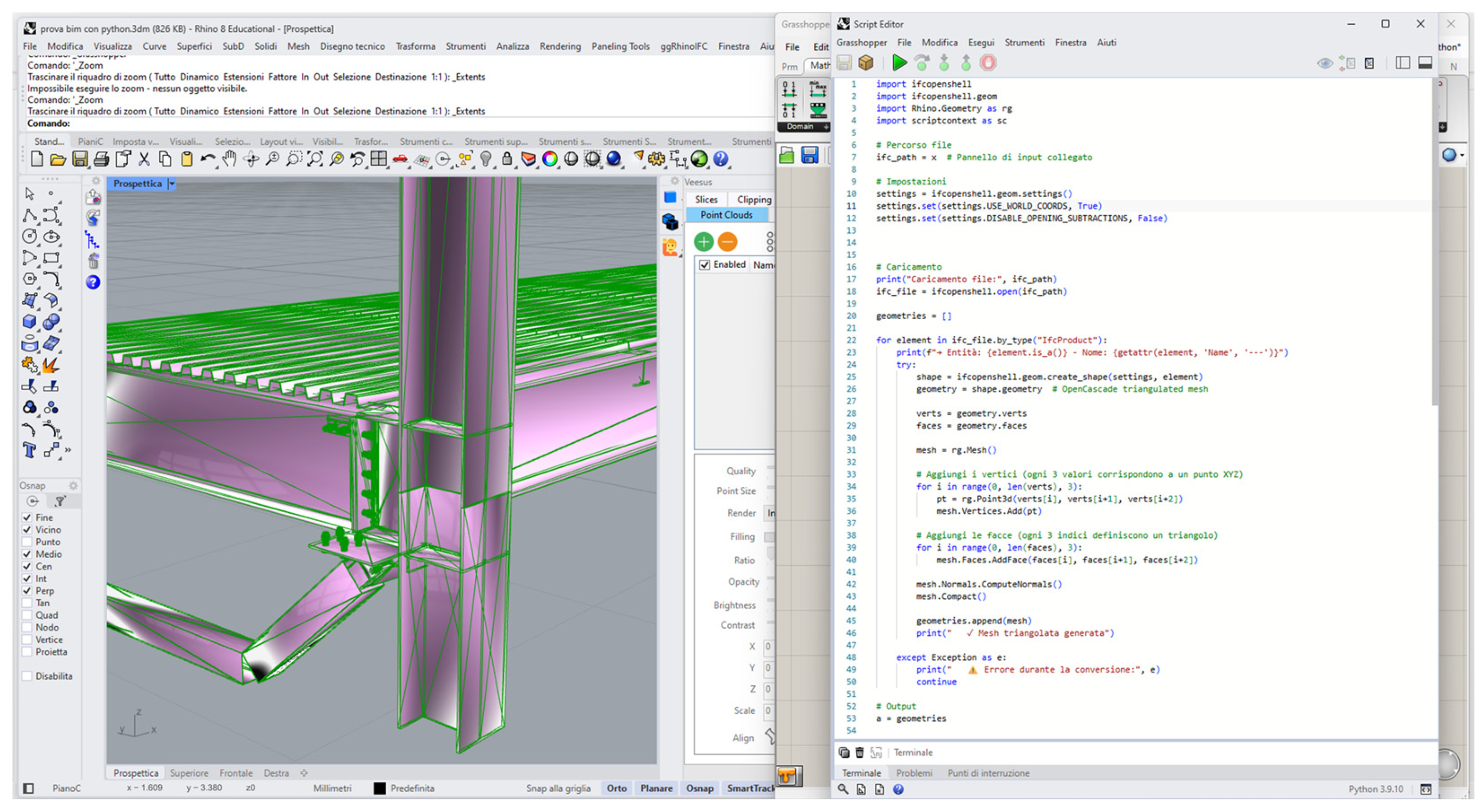
This step directly prepares the geometries for extrusion and sweeps operations. The automated process continues within Grasshopper, where three-dimensional geometries are created through the extrusion of sections along single axes (single-track sweep), multiple axes (double-track sweep) or networks of curves (network surface), generating parametric surfaces and solids. Integration with the pipeline continues with an automatic STEP/IFC export phase that allows geometric BrIM/FEM models to be transferred consistently while maintaining traceability from the point cloud to the section and the extruded geometry. The proposed workflow is used to transfer a structural model created in MIDAS CIM/BrIM, whose native output formats are limited to IFC and Parasolid, into a clean, hierarchical STEP dataset ready for use in FEM environments, with a particular focus on COMSOL and plate fatigue analysis (
Appendix B).
The transition from survey-based BrIM generation to FEM-oriented structural analysis cannot be achieved through file export alone. Instead, the model must be cleaned, organised, and transformed through a multi-software workflow in order to obtain a coherent and interoperable dataset suitable for simulation. This need arises from an interoperability constraint: IFC and Parasolid alone are not sufficient to manage the required transformations (classifications by type, perforations, axis extraction, robust sections). A hybrid pipeline was therefore adopted. Rhinoceros, through Python scripting, was used as a “connector” when a quick and reliable conversion to STEP was required. FreeCAD, in turn, was used as the procedural modelling environment in which the data structure was consolidated, section cuts were automated and Boolean operations not natively supported by CIM for the analysed case study were applied, particularly for the repeated drilling of plates based on the bolt layout. For this reason, the first architectural decision was to normalise the hierarchy. In the FreeCAD document, homogeneous source groups (STRUCT_BEAMS_SRC001, STRUCT_COLUMNS_SRC001, STRUCT_BRACES_SRC001 and STRUCT_PLATES_SRC001) were introduced as the sole containers of load-bearing solids, keeping the nomenclature consistent with the discipline (beams, columns, braces, plates). In parallel, the AXES_* tree was created for geometric axes (AXES_BEAMS, AXES_COLUMNS, AXES_BRACES) and, subsequently, a specific branch for bolt axes, which proved essential for plate drilling and geometric checks.
3.5. Automated Bolt-Based Plate Perforation Pipeline
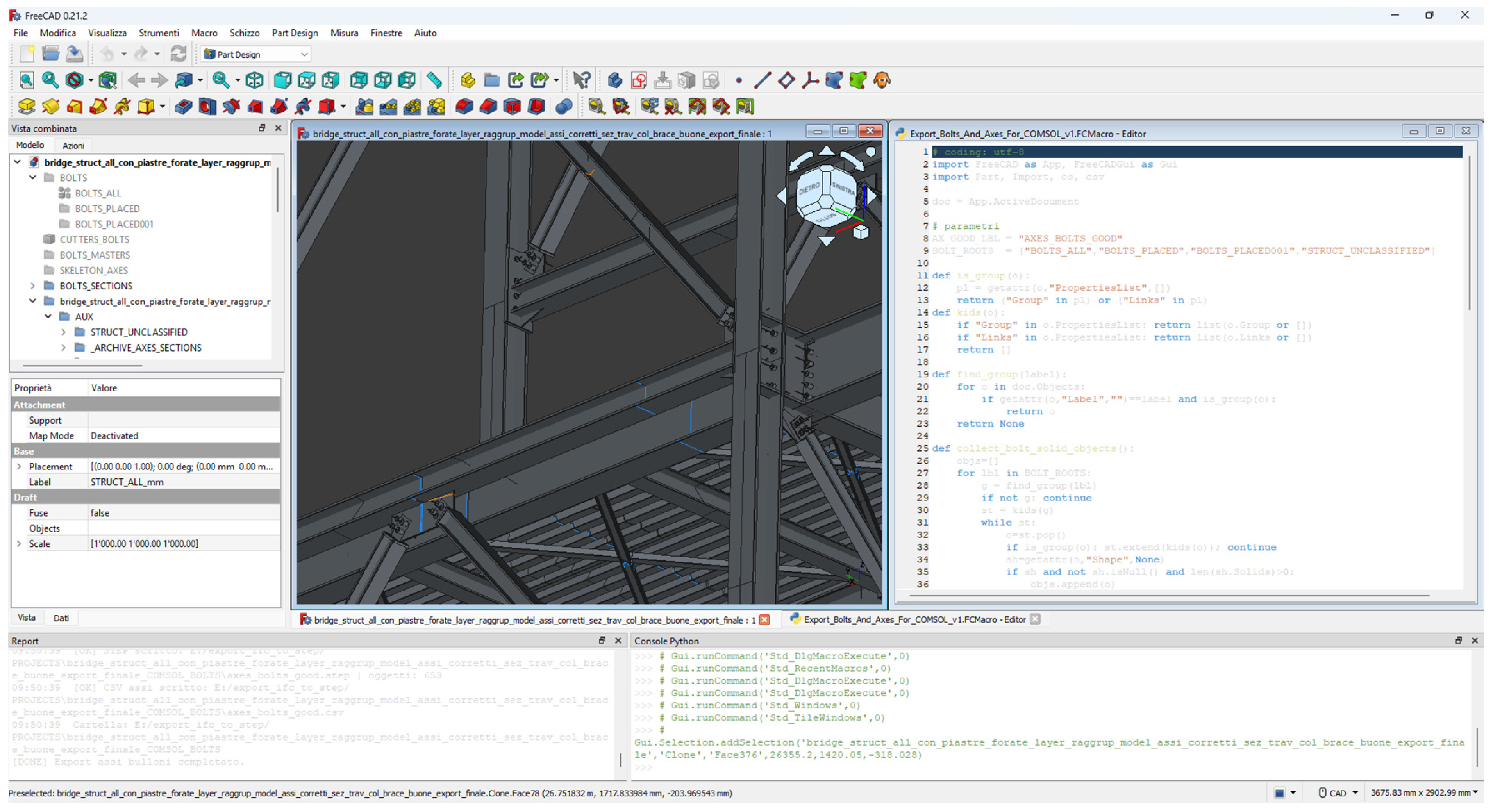
The treatment of bolts was a key aspect of the workflow, since it directly affects plate perforation and, downstream, fatigue analysis. The original model did not provide bolts as uniformly usable solids; therefore, work was carried out on the axes, using them both as positioning references and, after appropriate trimming, as parametric tools to generate the holes. The raw collection of candidates (thousands of objects) was filtered using a three-stage procedure: (i) deduplication and controlled copying in AXES_BOLTS, (ii) geometric cleaning and moving to AXES_BOLTS_CLEAN; (iii) separation into “good” and “outliers” according to criteria of length, straightness, proximity to plates and consistency of inclination. This normalisation gave rise to the AXES_BOLTS_SHORT set, which was subsequently refined in AXES_BOLTS_GOOD. Starting from this phase, it was possible to perform massive drilling: the GOOD axes were used as generators of cutting cylinders (CUTTERS_BOLTS) applied to the structural group of plates, to obtain, in a differentiated but repeatable way, the Boolean subtraction of plate-bolt that CIM did not provide in the original workflow. The entire process was implemented through dedicated macros and verified through the additional Python console available in FreeCad (
Figure 13).
This step, in addition to drastically reducing ambiguities during the FEM meshing phase, resulted in a digital as-built model consistent with the construction geometric details required for fatigue calculations. Once the pipeline of sections and holes had been stabilised, the approach to data export was organised. To ensure reuse and traceability, the STEP files were issued by families, keeping labels and containers consistent with the FreeCAD tree: beams.step (120 objects), columns.step (34), braces.step (25) and plates.step (439), accompanied by the corresponding axes as STEP curves (axes_beams.step, axes_columns.step, axes_braces.step) and the CSV summary of global axes (axes_all.csv). For bolts, at the end of the cleaning process, axes_bolts_good.step and axes_bolts_good.csv were produced, so as to have precise references for constraints and contacts or to generate, on the solver side, reduced entities (beam/truss/edge) associated with the actual bolts. The added value of this segmentation is twofold: it allows for selective imports (e.g., testing only the plate with holes and bolt axis) and makes the quality control steps transparent, since outliers remain tracked and isolated. On the COMSOL side, a skeleton project with an explicit data structure has been set up: a COMSOL_PROJECT folder that hosts data/_COMSOL/for structural geometries and data/_COMSOL_BOLTS/for bolt axes. The skeleton also contains a Java script (executable from the interface or in batch mode) that standardises the unit to millimetres, imports the various STEPs (solids and curves), creates “placeholder” selections for beams/columns/braces/plates and for sets of axes, and offers extension points for any solid unions or automatic definitions of Selections functional to meshing and Physics. Alternatively, the “GUI-only” route remains straightforward: 3D model, units set to millimetres, import of the four structural STEP files with standard options (without Combine objects, Repair by default), import of the three axis files and the axes_bolts_good.step set, saving, and, if required by the problem, union of volumes via Form Union with control of internal boundaries. In both cases, the presence of clean and semantically separated STEP files reduces import times and, above all, eliminates the topological uncertainties that cause the mesh failures typical of traditional BIM models.
From a methodological point of view, the central element of this approach was the transformation of a “BIM-as-is” dataset into a simulation-ready dataset governed by three principles: (i) strong classification (structural sources and sets of axes/sections in dedicated trees, with stable labels); (ii) robust geometry (section cuts with fallback and along-axis scanning, controlled tolerances, repeatable Booleans); (iii) modular export (STEP per family and curves/CSV of axes for constraints, controls and automations). The analysed case study, consisting of 120 beams, 34 columns, 25 braces, 439 plates and several hundred bolt axes. Its relevance lies less in the numerical result itself than in demonstrating that, even when the source software does not directly provide the operations required by the calculation, a reliable and industrial sable workflow towards FEM codes can still be established while maintaining quality control at every stage. Ultimately, the entire workflow was designed to maximise repeatability (macros and folder conventions that can be reused on similar models). It is precisely this repeatability that makes it possible to tackle advanced analyses such as plate fatigue in COMSOL: the plates are already perforated, the bolt axes are available for constraints/locations, and the structural families can be separated for different loads and boundary conditions. The transition from IFC/Parasolid “design” to STEP “calculation” is therefore not merely a format conversion, but the construction of a common language between BIM and FEM, in which geometry, semantics, and automation become three sides of the same workflow. For completeness, the upstream geometric modelling environment used to generate the parametric BrIM model is briefly summarised below.
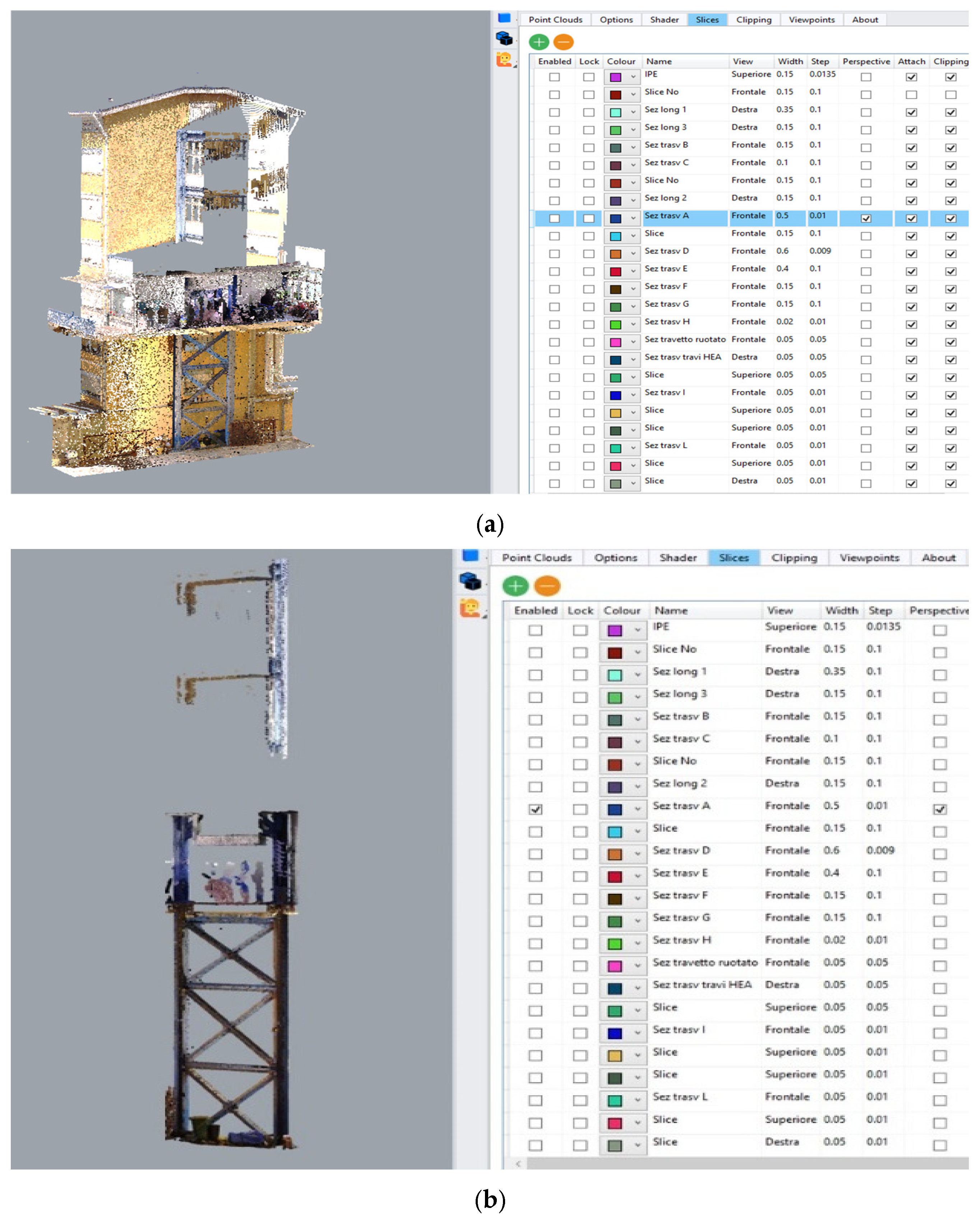
The classified part of the point cloud was imported into the Rhinoceros environment using the open and standardised E57 format, which allows the acquisition metadata and the original reference system to be retained. To manage large datasets more efficiently, the cloud is immediately converted to the proprietary Veesus (.vpn) format, which is compatible with the Arena4D plug-in. This conversion allows for the use of advanced rendering and navigation features, varying the display with transparency schemes or RGB colour mapping to facilitate the interpretation of the detected morphologies. Arena4D is then used to define section planes, which can be freely oriented in space and generated according to geometric restoration requirements. The horizontal planes are used to intersect the cloud at the floor levels, from which the sections of beams and pillars are derived; the vertical planes allow the transverse frames to be reconstructed and significant areas such as centre lines and supports to be analysed; finally, the oblique planes are indispensable for documenting the horizontal bracing of the floors and the vertical bracing of the frames. The intersection of these planes with the cloud produces shapes on which polylines and splines are drawn, representing the actual sections of the structural elements. All the entities produced are then organised into dedicated disciplinary layers, which allow the different families of components to be distinguished and ensure traceability in the subsequent BrIM geometric modelling phase. The surveyed structure has three decks and five vertical braced frames, consisting of pillars and braces. The road axis is described according to a plano-altimetric definition, with reference stations used to constrain the generation of the deck.
Figure 14 shows a general view with some sample sections and elevations and the management of “Slices” for 2D derivation.
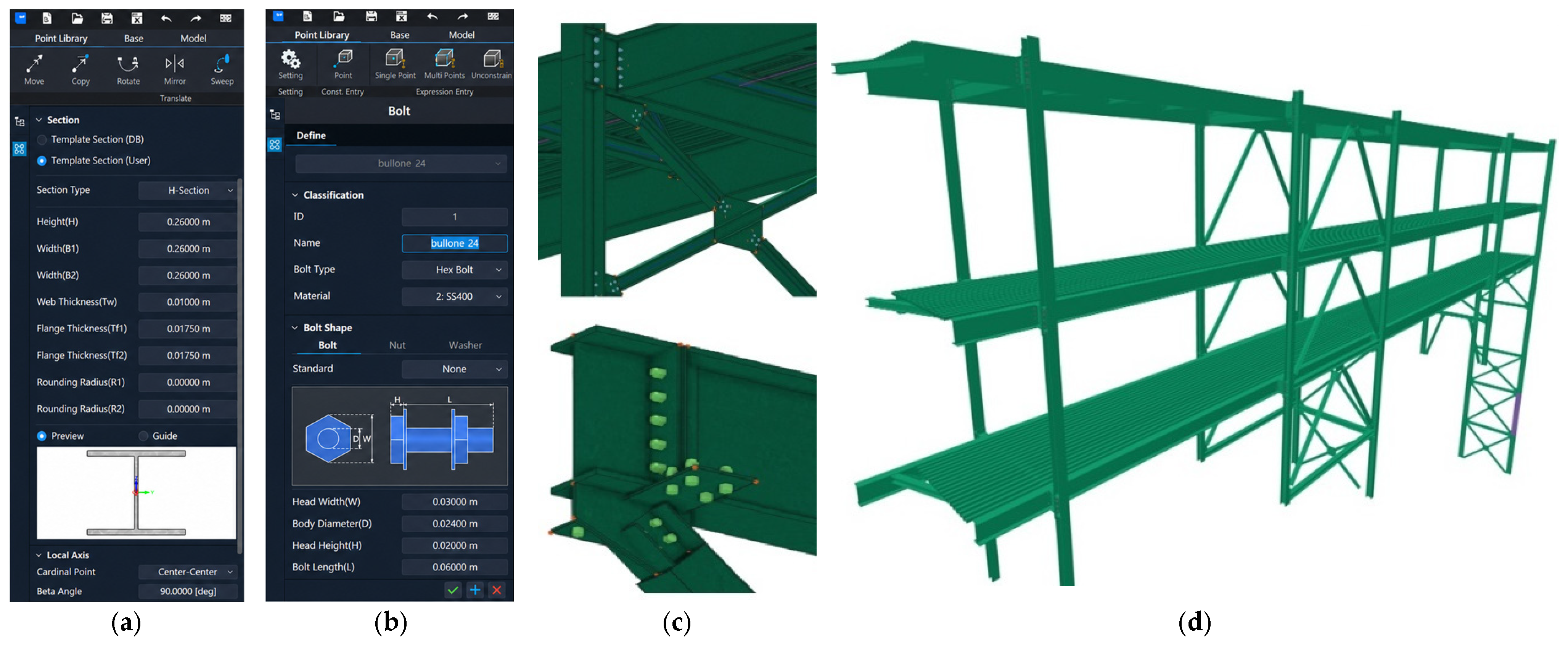
In Rhinoceros, layers organise sections, axes, and dimensions for verification; control dimensions define tolerances and populate the QA/QC register, while Veesus slicing yields clean polylines for 3D modelling. The point cloud and sections are then imported into MIDAS CIM, keeping the georeferenced system and aligning the model to the global Cartesian axes. Here, elements are rebuilt from curves and axes using Booleans and sweep/loft/extrusion operations to obtain editable solids. Components are immediately structured into the Point and Curve libraries and Assembly Units within a project library, becoming parametric information objects with attributes and relationships.
This parametric approach allows any plano-altimetric changes to the axis or sections to be automatically propagated to the entire model, consistently updating beams, frames, slabs, plates and bolts. In addition to improving modelling efficiency, this method ensures perfect consistency between geometric and informational data, which is essential for any subsequent analyses and simulations.
Figure 15a shows an example of a parametric steel section, while
Figure 15b shows the bolt library with geometric and material parameters.
Figure 15c,d show details of the frame and details of the bolted connection between the beam and the wind brace. The BrIM hierarchy adopted is organised in the Worktree. This documents the information structure and allows for traceability. It lists the Point Library (with the main cross-sections and longitudinal sections), the Curve Library (containing the deck guide curves), the Assembly Units (for frames and modular decks) and the Material entries, which can also be updated based on the results of in situ tests.
Data interoperability is ensured through the use of multiple exchange formats and environments, including georeferenced LAS/LAZ for point clouds, 3D CAD for curves/sections/axes, Parasolid and IFC4 for model exchange and Midas Gen for structural analysis. The visualisation of the completed BIM (
Figure 15d) is shown in Sortdesk IFC Viewer, a free browser-based tool for exploring IFC models.
3.6. Preliminary Structural Application
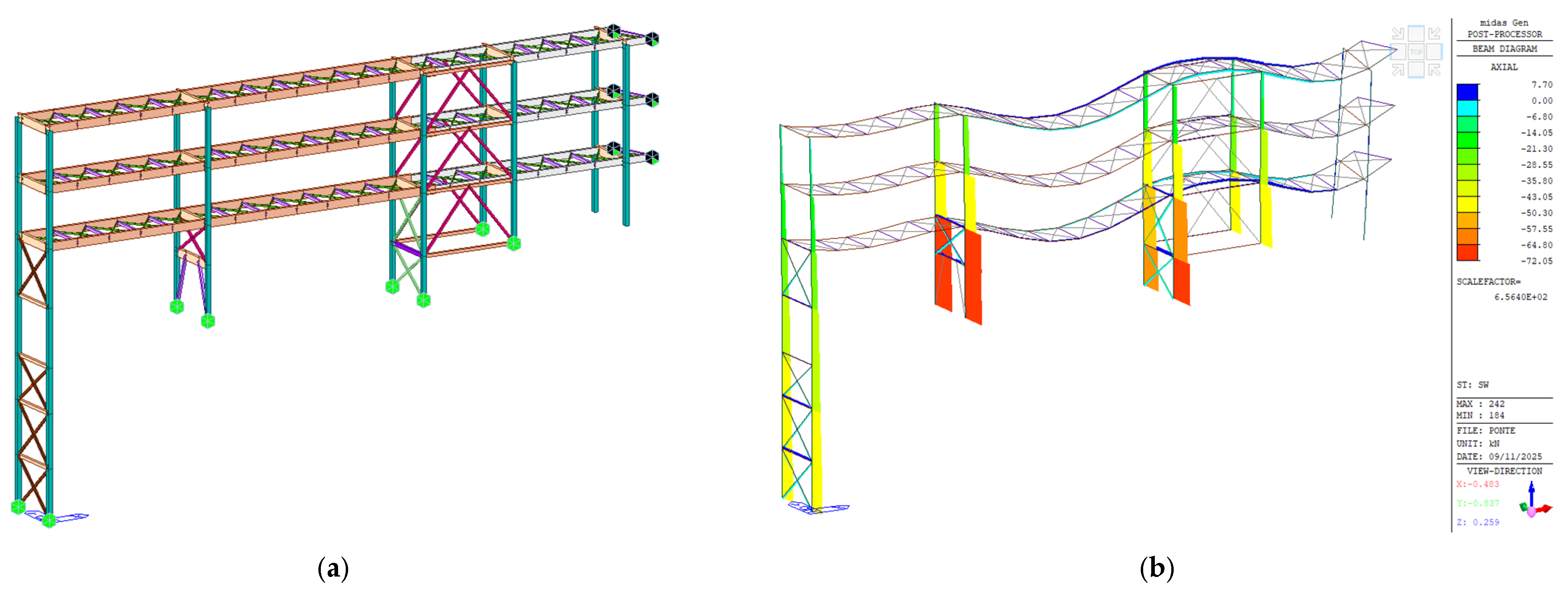
A preliminary structural application of the proposed interoperability workflow was carried out by transferring the as-built bridge model into the FEM environment of Midas Gen. The primary objective of this phase is not to provide a fully structural assessment, but rather to demonstrate the consistency, usability, and interoperability of the generated Scan-to-BrIM model within a structural analysis framework.
Figure 16a,b show the resulting analytical model and a representative output of the preliminary structural application. In the analytical model, the main horizontal members, purlins, and columns were modelled as beam elements, while most bracing members were represented as truss elements. The X-bracing system was instead modelled using beam elements with flexural releases at the frame intersections, in order to account for connections not capable of transferring bending moments. The section properties adopted in the structural model were derived from the BIM model developed from laser-scanner survey and point cloud processing. Boundary conditions were assigned consistently with the observed structural behaviour: the column bases were assumed to be fully connected to the ground, whereas, on the cantilever side towards the Radiology block, the connection between the bridge and the main structure was modelled as a vertical roller able to transfer vertical loads only.
Figure 16b reports a representative axial-force distribution under self-weight, confirming that the transferred model can be effectively used for downstream structural analyses. From a qualitative engineering perspective, the axial-force distribution matches the expected behavior of a steel frame bridge under self-weight: vertical members mainly carry compression, bracing elements handle both tension and compression for stability, and horizontal members transfer loads. This agreement supports the preliminary consistency of the geometric and structural modeling. However, quantitative validation was not possible due to the absence of reference data such as design models, material properties, or field measurements, preventing direct comparison of structural results. Furthermore, several sources of uncertainty affect the current analysis. These include the limited knowledge of material properties, the simplification of boundary conditions, and the assumptions made in the structural idealisation (e.g., beam and truss representations). In particular, the mechanical properties of the steel members were assumed based on typical values rather than verified through testing, which may influence the accuracy of the results. The analyses did not reveal significant issues under static actions, whereas some non-verifications persisted in the bracing system under seismic assessment, reflecting the remaining uncertainty in the material properties and cross-sections of these members despite the survey campaign. Although the analysis remains preliminary because of limited material knowledge and simplified load assumptions, it demonstrates that the proposed Scan-to-BrIM workflow can effectively support downstream FEM applications and enable structurally meaningful use of the reconstructed model. Future developments will focus on integrating material testing data, refining boundary conditions, and validating the model against experimental or design references to enable more rigorous structural assessments.
4. Discussion and Conclusions
The proposed methodology enabled the generation of an accurate as-built BrIM model of an existing steel structure by coupling (i) a calibrated survey strategy with (ii) an end-to-end, geometry-aware automation pipeline from point cloud to BrIM/FEM-ready outputs. During acquisition, dense point clouds were produced with limited user intervention once scanning parameters were tuned to the required level of detail. Although registration can be manual, semi-automatic, or automatic, current practice increasingly relies on automated matching (e.g., ICP variants and feature-based methods) to manage large datasets efficiently. In this study, FARO Scene provided a particularly effective registration workflow by integrating target-based, cloud-to-cloud, and top-view strategies with strong automation, reducing manual effort compared with commonly used alternatives [
29].
Although the proposed workflow demonstrated strong applicability for the investigated steel bridge, direct generalization to other bridge typologies (e.g., masonry arch bridges, reinforced concrete bridges, deteriorated structures) may require recalibration of segmentation and modelling parameters. The results demonstrate the feasibility of the proposed workflow for generating simulation-ready BrIM models from point cloud data. While the approach improves reproducibility and reduces manual intervention, further validation and benchmarking are required to fully assess its performance across different structural scenarios. The method, indeed, is not intrinsically limited by the overall length of the structure since the pipeline is based on a modular and locally driven logic.
The performance of the method is strongly dependent on the quality, density, and completeness of the input point cloud. In highly noisy environments, such as operational facilities with moving people, reflective surfaces, or temporary obstructions, clustering, axis estimation, and section extraction may become less stable, potentially leading to local misclassification of structural elements or inaccurate reconstruction of secondary details. Similarly, incomplete scans and severe occlusions may affect the continuity-based aggregation of structural components, especially for partially visible braces, hidden connections, or local construction details that are not sufficiently represented in the point cloud. A further limitation concerns the use of threshold-based decision rules. Although the adopted thresholds are linked to point cloud density, voxel size, feature scale, and preliminary calibration tests, their effectiveness may vary under different acquisition conditions. Therefore, the workflow should not be interpreted as a fully autonomous black-box procedure, but as a semi-automated and controllable pipeline in which parameter settings must be verified against the quality of the acquired data and the required level of geometric detail.
Preliminary tests confirmed that resolution, quality, and acquisition distance directly affect the readability of small structural details (bolts, welds). Short-range scans (≈2 m) with higher settings produced sufficiently dense clouds for reliable detail recognition, whereas increasing distance led to a progressive loss of definition. Consequently, survey parameters were not optimised solely for speed, but adapted to local constraints through a modular strategy: medium settings for accessible areas requiring detail, faster settings where continuity and operational constraints dominated, and higher resolution for distant roof acquisitions. In dynamic environments such as hospitals, noise and occlusions remain partly unavoidable (traffic, reflections), but consistent quality settings and careful scan planning provided a robust basis for subsequent filtering and segmentation. The photographic component further improved interpretability (structural vs. services/finishes) and enabled a virtual tour that supported remote inspection and reduced repeated site visits. Beyond acquisition, the main contribution lies in converting an as-is point cloud dataset into a simulation-ready dataset through a highly automated pipeline that is less dependent on manual fitting and operator experience than many traditional Scan-to-BIM workflows [
30,
31]. Compared with approaches that automate only specific sub-tasks (e.g., steel frame reconstruction) or remain partially manual [
32,
33], the workflow introduces: (1) data-driven frame selection using an explicit scoring scheme (section flatness, element co-occurrence, continuity across slicing, support density, including double-C coupling checks); (2) automatic construction of normalised orthogonal axes and slicing planes for consistent section extraction and parametric modelling; and (3) a structured export strategy that preserves traceability from point cloud to sections to solids. In practice, the chain integrates Python/Anaconda for classification and axis recognition, Rhinoceros/Grasshopper for parametric reconstruction, and automated post-processing in FreeCAD to reorganise elements into families, clean and generate axes, manage plate perforations from bolt axes, and export interoperable, semantically structured STEP/CSV datasets. This reduces import ambiguity and meshing failures typical of BIM-derived geometries, while improving repeatability through standardised naming, folder conventions, and scripted exports. Compared to recent Scan-to-BrIM approaches proposed in the literature, the main contribution of this work lies in the integration of multiple processing stages into a unified and reproducible workflow. While methods such as those proposed by Noichl et al. (2025) [
11] focus on advanced geometric reconstruction and topology extraction, and other studies address specific tasks such as segmentation or BIM updating, the proposed approach provides a direct link between reality capture and FEM-ready models. This integrated perspective is particularly relevant for engineering applications, where interoperability and model usability are critical.
The workflow demonstrates that a reliable and industrialisable pipeline from reality capture to BrIM and FEM applications can be achieved, even when source software lacks direct FEM-oriented preprocessing capabilities. The preliminary structural application in Midas Gen confirms the usability of the generated as-built model for downstream analysis. The approach is replicable across steel structures and provides an efficient pathway to interoperable, analysis-ready models with reduced manual effort. This end-to-end automation represents a key innovation of the proposed Scan-to-BrIM workflow.
The methodology shows promising results but has several limitations. Its performance depends heavily on point cloud quality and density, with low resolution affecting the detection of fine details like connections. It is also sensitive to occlusions and incomplete data, which can reduce reconstruction accuracy in complex environments. The approach assumes standard steel profiles, limiting its use for irregular geometries. Additionally, the structural analysis remains preliminary due to the lack of validation with experimental data or design models. Future work will aim to integrate multi-source data, enhance robustness in challenging conditions, and validate results through comparison with real measurements and documentation.




 ,
,