Analysis of Structural Contact and Collision Behavior Based on Member Discrete Element Method for Large-Span Structures

Abstract

Large-span structures may experience progressive collapse involving complex member collisions, for which efficient and accurate simulation remains a challenging problem in engineering practice. Conventional finite element methods are computationally inefficient in such scenarios due to repeated reconstruction of contact constraints and global stiffness matrices, while existing member discrete element method (MDEM) approaches lack a unified contact algorithm capable of handling both “point–line” and “line–line” contact modes. To address these limitations, this study extends the MDEM framework for structural collision analyses by establishing unified “point–line” and “line–line” contact models. A “virtual contact point pair” concept was introduced to define critical contact constraints, and corresponding contact force formulations were derived. A Fortran-based computational program was developed. Numerical validation through typical examples showed that the maximum relative error was 4.2% for the elastic ring problem and 3.1% for the double cantilever beam, while the rebound angle deviation in the flexible ring impact case was less than 2°. The proposed method avoids global stiffness matrix reconstruction and achieves a 95–98% accuracy compared to reference solutions under recommended parameters, providing an efficient approach for simulating member collisions in large-span structural collapse and supporting engineering analyses and design.

1. Introduction

During the structural collapse process, contact and collision between members naturally occur as physical phenomena. Accurately calculating the contact and collision interactions between members during the large deformation phase is essential for simulating structural collapse.

For contact and collision problems, accurately calculating the contact force is crucial, as it directly determines the precision of the simulation results. In the finite element method (FEM), a contact force calculation typically employs the Lagrange multiplier method, the penalty method, and the defense node method. The Lagrange multiplier method [1,2] can precisely satisfy constraint conditions, but increases the degrees of freedom in the governing equations, complicating the solution process and creating incompatibility with explicit time integration schemes. The penalty method [3,4] does not require increasing the problem’s degrees of freedom and is widely used due to its simple logic and ease of implementation. However, constraint conditions are often only approximately satisfied, and the calculated contact forces are significantly influenced by the choice of the penalty factor, leading to instability in the solution process. Currently, there is no clear criterion for selecting the penalty factor. In contrast, the defense node algorithm proposed by Zhong [5] is compatible with explicit time integration and can precisely satisfy local contact constraints by using Lagrange multipliers.

Unlike the FEM, the theoretical foundation of the discrete element method for member systems (MDEM) is non-continuum mechanics. This approach was proposed by Ye [6] based on traditional particle discrete element methods and has been successfully applied to continuous medium problems. This approach represents structural members as discrete rigid spheres whose dynamics obey Newton’s second law. The interaction between adjacent particles is characterized by contact constitutive models, establishing the basic simulation unit termed the contact element. The MDEM not only extends the applicability of traditional discrete element methods, but also retains their advantages: no need to assemble a global stiffness matrix or iteratively solve the motion equations. This approach has been successfully validated in multiple aspects of structural analyses, including geometric nonlinearity in framed structures [7,8], material nonlinear behavior [9,10], semi-rigid joint modeling [11,12], nonlinear dynamic response analyses [13,14,15], structural buckling phenomena [16], and collapse simulation of reticulated shells [17,18,19,20]. These achievements demonstrate that the MDEM has unique advantages in simulating complex behaviors such as large geometric deformations, material nonlinearity, and fracture collapse, making it a simple and effective approach for studying structural nonlinearity and fracture behavior.

In summary, existing contact force calculation methods in the finite element framework—such as Lagrange multiplier methods, penalty methods, and constraint-based approaches—are well established, but they face limitations, including increased degrees of freedom, difficulty in selecting penalty factors, and incompatibility with explicit time integration. While the MDEM framework offers advantages for large-deformation and collapse simulations, its application to member-level collision analyses remains limited. Specifically, a unified algorithm capable of handling both “point–line” and “line–line” contact modes within the MDEM framework is currently lacking. To address this gap, this study proposes a virtual contact point pair-based MDEM for contact–collision analyses, which enables efficient and consistent treatment of multiple contact modes in structural collapse simulations.

Although DEM-based methods have been widely applied to contact–collision problems, certain limitations remain in the existing approaches. Recent studies have noted that penalty-based contact algorithms in the combined finite-discrete element method (FDEM) may exhibit element-size-dependent behavior and non-smooth contact force transitions [21]. Similarly, improved Metaball DEM formulations have been reported to encounter convergence difficulties when handling complex contact geometries [22]. In the context of large-span structures, where beam and truss elements are prevalent, most existing contact detection algorithms were developed primarily for polyhedral or spherical particles [23,24,25]. Therefore, a contact model that is computationally efficient and avoids iterative convergence procedures would be desirable for this class of problems.

To this end, this study proposes an MDEM-based contact–collision analysis method using virtual contact point pairs, aiming to extend the applicability of the MDEM to the analysis of collision behavior in member systems. The specific research tasks included: (1) establishing “point–line” and “line–line” contact models suitable for the MDEM framework; (2) deriving the contact force formulations based on non-penetration constraints; (3) developing the corresponding computational program; and (4) validating the accuracy and effectiveness of the proposed method through representative numerical examples.

2. The Theory of MDEM

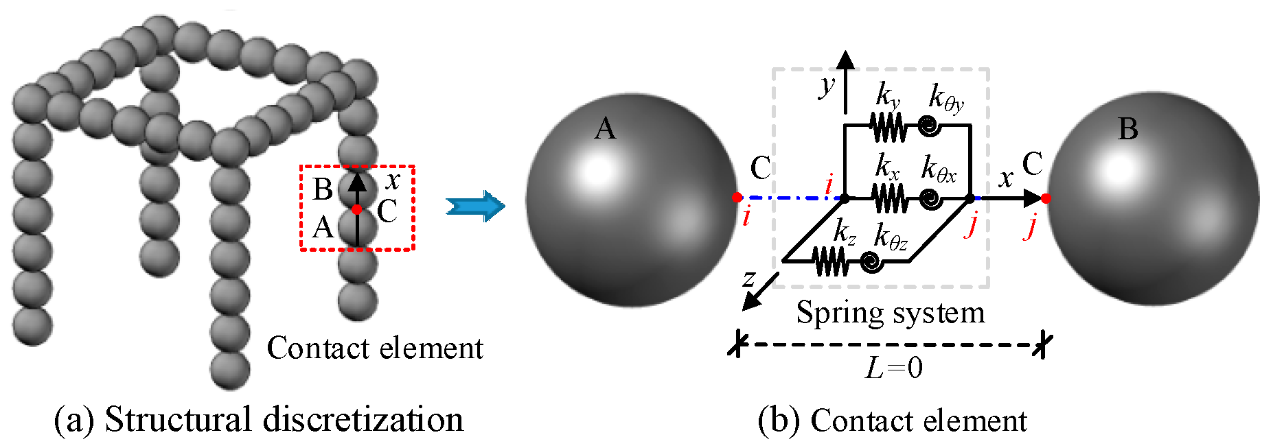
For a detailed derivation of the fundamental theory of the MDEM, readers are referred to References [6,7,8]; only a brief overview is provided in this section. The MDEM divides the structure into a finite set of rigid particles, as shown in Figure 1a. Adjacent particles (such as particles A and B) are connected by a zero-length spring system, forming the basic analysis unit—contact elements, as shown in Figure 1b.

The solution framework for the MDEM mainly consists of two parts: the solution of the motion equations and the computation of internal forces. A brief explanation is provided below.

Figure 1. MDEM model for framed structures.

Figure 1. MDEM model for framed structures.

2.1. The Governing Equation

At any moment t, the motion of all particles in the discrete element model of the member system follows Newton’s second law. The motion control equations are as follows:

$$\left\{\begin{array}{l}M\ddot{u}(t)+C_M\dot{u}(t)=F^{ext}(t)+F^{int}(t)\\ J\ddot{\theta }(t)+C_J\dot{\theta }(t)={\overline{M}}^{ext}(t)+{\overline{M}}^{int}(t)\end{array}\right.$$

(1)

where M and J represent the equivalent mass and equivalent moment-of-inertia matrix of the particles in the global coordinate system, respectively. $\ddot{u}$ and $\ddot{\theta }$ represent the translational and rotational accelerations of the particles, respectively. $\dot{u}$ and $\dot{\theta }$ represent the translational and rotational velocities of the particles, respectively. $F^{ext}$ and ${\overline{M}}^{ext}$ are the external forces and moments, respectively; $F^{int}$ and ${\overline{M}}^{int}$ are the internal forces and moments, respectively. C_M and C_J represent the translational and rotational damping matrices, respectively. In this study, they are defined as $C_M=\alpha M$ and $C_J=\alpha J$, where α denotes the mass-proportional damping coefficient. The parameter α was taken as 0.7 in this study based on preliminary trial calculations. Under this value, structural responses in representative examples showed a good agreement with the literature results (see Section 6). For practical applications, it is recommended to perform sensitivity analyses of the damping parameter for specific problems to ensure robust results.

Using the central difference method to solve Equation (1), the translational velocity and acceleration of each particle can be expressed as follows:

$$\left\{\begin{array}{l}{\dot{u}}^t={\displaystyle \frac{1}{2}}({\dot{u}}^{t-\Delta t/2}+{\dot{u}}^{t+\Delta t/2})\\ {\ddot{u}}^t={\displaystyle \frac{1}{\Delta t}}({\dot{u}}^{t-\Delta t/2}+{\dot{u}}^{t+\Delta t/2})\end{array}\right.$$

(2)

Substituting Equation (2) into Equation (1) gives the translational velocity of the particle at time t + Δ/2. Consequently, the translational displacement of the particle at the next time step can be obtained as follows:

$$\begin{array}{l}{u}^{t+\Delta t}=u^t+{\dot{u}}^{t+\Delta t/2}\cdot \Delta t\\ \hspace{1em} =u^t+{\displaystyle \frac{c_2}{c_1}}\cdot \Delta t\cdot {\dot{u}}^{t-\Delta t/2}+{\displaystyle \frac{\Delta t^2}{c_1}}\cdot {\displaystyle \frac{1}{m}}\cdot (F^{ext,t}-F^{int,t})\end{array}$$

(3)

where $c_1=1+0.5\cdot \alpha \cdot \Delta t$; $c_2=1-0.5\cdot \alpha \cdot \Delta t$; m is the mass of the particle.

Similarly, the rotational displacement of each particle can be obtained, and will not be elaborated further.

2.2. Calculation of Internal Forces in Contact Elements

From the discrete process of the structure shown in Figure 1a, it can be inferred that the contact elements are equivalent to beam elements in traditional finite element methods. The deformation and material properties of the entire beam element are characterized by a zero-length spring system at the contact point between two rigid particles, as illustrated in Figure 1b. The two nodes of the zero-length spring system are connected to the contact point C on the edges of the two particles. The six springs are independent and uncoupled, representing three translational and three rotational degrees of freedom of the contact element. After obtaining the velocities and displacements of particles A and B from Equation (1), the relative displacement increment of the two nodes of the spring system can be further derived using kinematic theory. By utilizing the contact constitutive relation given in Equation (4), the internal force increment at contact point C can be calculated. Finally, the internal forces at the centroids of particles A and B are obtained using the principle of force translation.

$$\left\{\begin{array}{l}\Delta f=k\Delta u\\ \Delta \overline{m}=k_{\theta }\Delta \theta \end{array}\right.$$

(4)

where $\Delta f$ and $\Delta \overline{m}$ are the increments in the internal force and internal moment at the contact point of the spring system, respectively; $k$ and $k_{\theta }$ are the translational and rotational stiffness matrices of the contact element, respectively, with values referenced in the literature [7]; and $\Delta u$ and $\Delta \theta$ are the increments in the translational and rotational displacements of the two nodes of the spring system in the local coordinate system, respectively. For the stability conditions and stiffness selection of the zero-length spring model, please refer to References [7,8].

3. Establishment of Contact Model

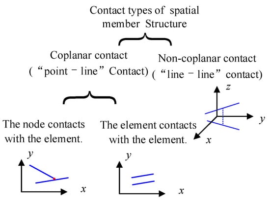
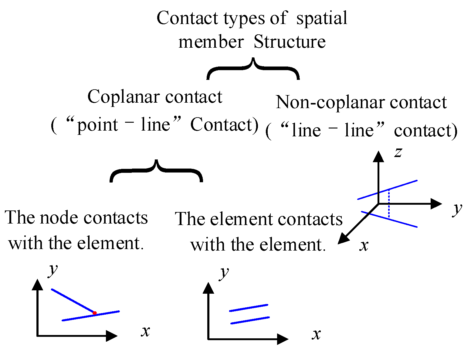
For spatial member structures, the potential contact types between members can be classified into two primary categories: coplanar contact and non-coplanar contact. Within coplanar contact, further subdivisions include intersecting and parallel configurations (the latter not being considered in this study), as illustrated in Figure 2. Accordingly, this study establishes corresponding “point–line” and “line–line” contact models, employing spatial analytical geometry vector analysis methods [26] to determine the relative positions between structural members accurately.

Figure 2. Element contact type of spatial member structure.

3.1. “Point–Line” Contact Model

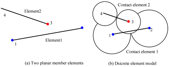
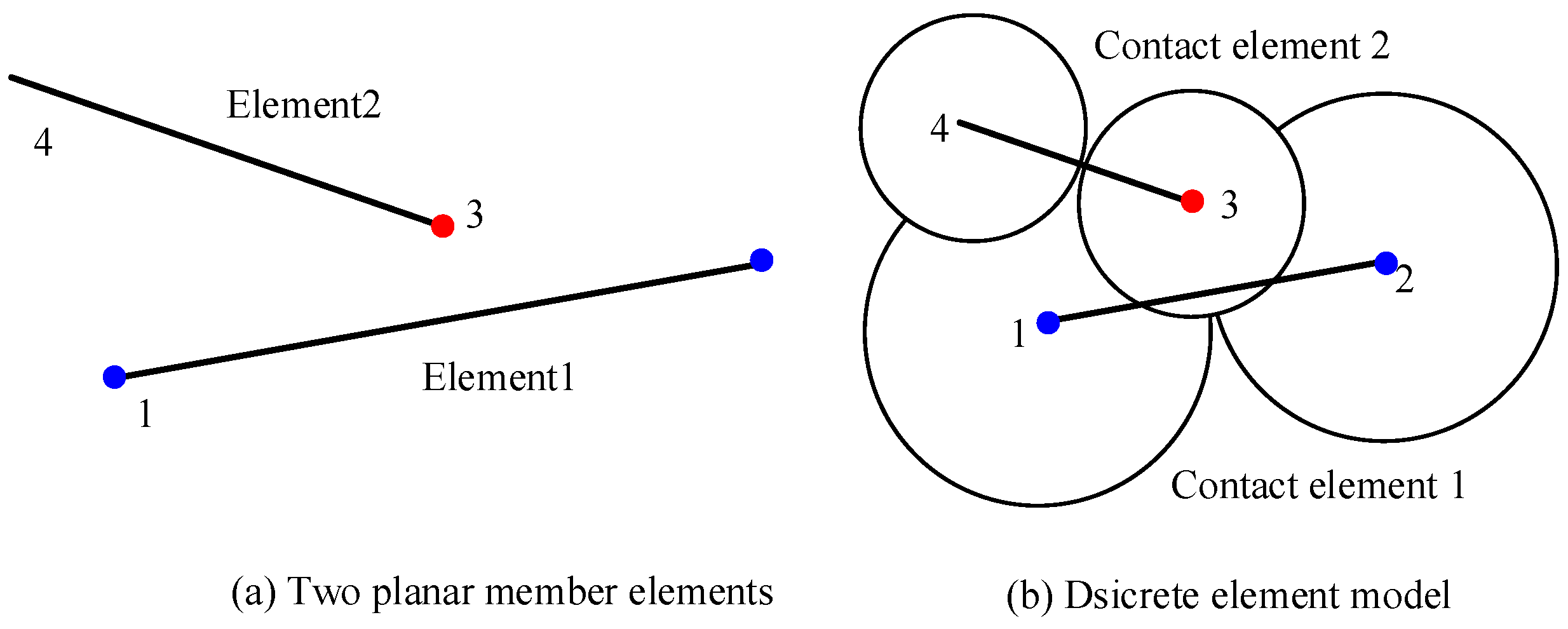
For the two member elements in the plane shown in Figure 3a, their discrete element analysis model corresponds to two contact units, with each node representing a spherical particle, as shown in Figure 3b. These spherical particles are hypothetical constructs for numerical simulation. In the discrete element model of Figure 3b, particle 3 may create a false contact phenomenon with element 1. Therefore, this paper employs the original model, as shown in Figure 3a, to determine whether contact occurs between member elements while using the discrete element model in Figure 3b for analyzing the responses of the elements.

Figure 3. Two planar member elements and MDEM analysis model.

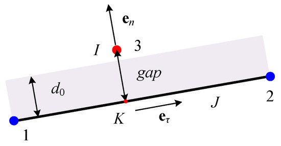
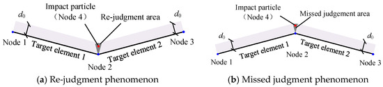
To determine whether the two member elements in Figure 3a are in contact, this section establishes a corresponding “point–line” contact model, as shown in Figure 4. Firstly, the impact particle I (node 3) is orthogonally projected onto the target element J’s axis, followed by a geometric verification of whether the projection point K lies within target element J. Secondly, to ensure that particle I does not penetrate target element J, the perpendicular distance between them, referred to as gap, is used as the contact discrimination parameter [27]. When the gap value is less than a specified threshold value d₀—that is, when particle I falls within the shadow area—contact is considered to have occurred. d₀ is the normal contact control constant introduced to avoid penetration due to computational errors. The parameter d₀ represents the allowable numerical penetration tolerance, introduced to avoid false contact detection caused by numerical round-off errors. A sensitivity analysis indicated that, when d₀ is chosen within the range of 10⁻⁵~10⁻³ times the characteristic structural dimension L, the variation in the computational results is less than 2%. An excessively small d₀ may lead to missed contact detection, whereas an overly large d₀ can introduce significant penetration errors. It is therefore recommended that d₀ be selected within the range of 10⁻⁵ L to 10⁻³ L. For the numerical examples presented in this study, d₀ was taken as 0.001–0.1 mm.

Figure 4. Point–line contact model.

Therefore, for the “point–line” contact model, the impact point must satisfy the following conditions for contact with the target element:

(1)

The projection point of the impact point must lie on the target element;

(2)

The perpendicular distance from the impact point to the target element, defined as the gap between the virtual contact point pair (I-K), must be less than a prescribed critical threshold d₀.

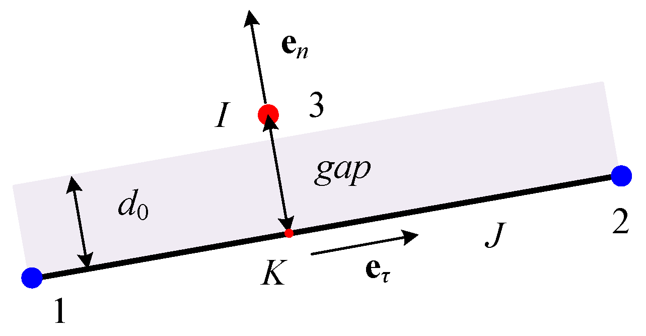
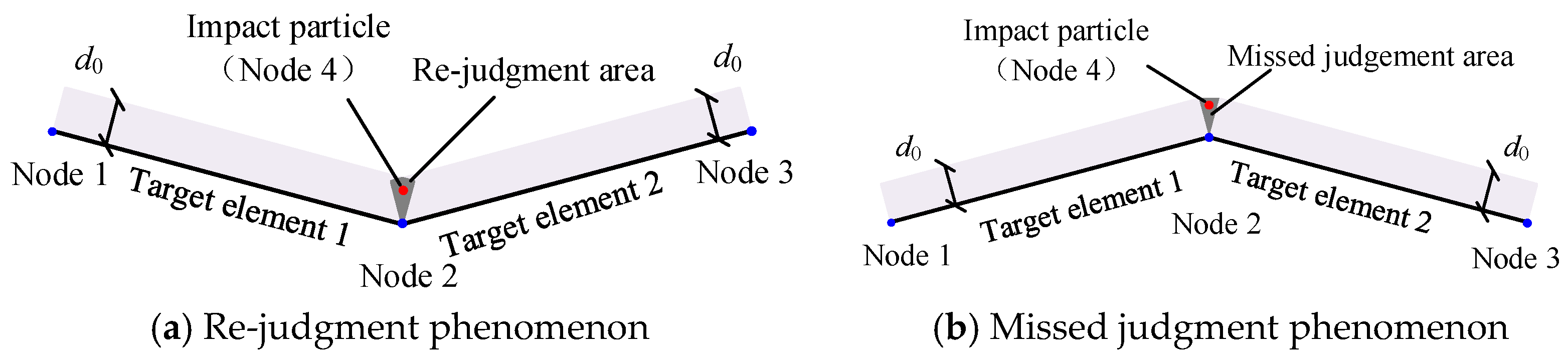
The “point–line” contact model established above is simple and easy to use, but it has extreme cases. As shown in Figure 5a, when target elements 1 and 2 are recessed toward the impact point, the projection of the impact point may fall within both target elements, leading to double counting. Conversely, when target elements 1 and 2 protrude toward the impact point, the projection may not fall within any target element, resulting in missed calculations, as shown in Figure 5b.

Figure 5. Special cases of projection algorithm.

To address this, the approach adopted in this paper was as follows: When the projection point lies within the proximal zones of the target element’s ends (i.e., the natural coordinate ξ of the projection point satisfies ξ ∈ [−Δd, Δd] ∪ [1 − Δd, 1 + Δd], where Δd controls the proximity threshold and is typically set to 0.01 or less), the impact particle (node 4) and node 2 form a virtual contact point pair. Under this condition, the “point–line” contact model degenerates to a “point–point” collision scenario.

To ensure continuity in contact detection and avoid double counting of contact forces, the following strategies were adopted: (1) When a projection point is close to the ends of two members, point–point contact is prioritized, and the original point–line pair is not recomputed. (2) Each contact pair follows a master–slave strategy, and forces are calculated only once. (3) Although the degeneration rules are heuristic, they effectively prevent numerical oscillations in contact states and are widely adopted in engineering practice.

It should be noted that the present projection method is based on a linear assumption and is applicable when the time step is sufficiently small. For strongly nonlinear paths, sub-stepping iterations or curved projection corrections may be introduced in future work.

3.2. “Line–Line” Contact Model

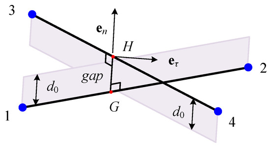
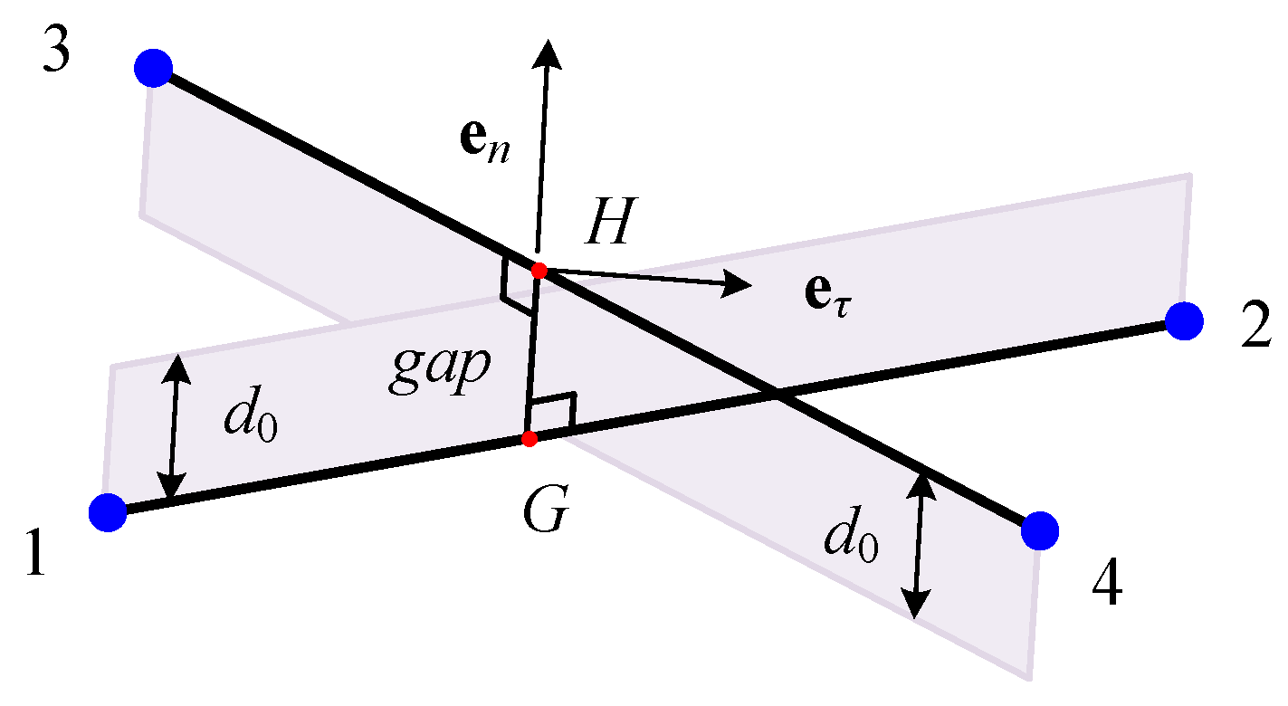
For the non-planar contact of spatial beam elements, this section establishes a “line–line” contact model, as shown in Figure 6. The closest points H and G (foot points) between beam element 1-2 (impact element) and beam element 3-4 (target element) form a virtual contact point pair. To prevent penetration, the shortest distance gap between them is used as the contact discrimination parameter. When the gap is smaller than a given critical threshold d₀, it indicates that contact has occurred.

Figure 6. Line–line contact model.

Consequently, the “line–line” contact model requires simultaneous satisfaction of two geometric criteria:

(1)

Both foot points H and G must lie within their respective element domains;

(2)

The orthogonal distance between the impact and target elements, defined as the gap of the virtual contact point pair (H-G), shall be less than the prescribed critical threshold d₀.

For the “line–line” contact model, extreme cases of re-judgment and missed judgment also exist. To address this, an analogous treatment was adopted: When the foot point H of the impact element lies near the end of the target element (i.e., its natural coordinate ξ satisfies ξ ∈ [0, Δd] ∪ [1 − Δd, 1]), the end particle of the target element replaces H, forming a virtual contact point pair with foot point G. The same logic applies in the reverse scenario (if G is near the end of the impact element). Under such conditions, the “line–line” contact model degenerates into a “point–line” contact formulation.

4. Contact Response Calculation

In this study, the contact response computation builds upon the defensive node algorithm proposed by Zhong and was adapted to the MDEM framework. A key feature of the proposed approach is the formulation of a closed-form non-penetration constraint based on “virtual contact point pairs” (see Equations (9) and (19)), which enables direct evaluation of contact forces without iterative procedures.

Compared with conventional finite element contact methods (e.g., node-to-surface contact and closest-point projection), the proposed approach exhibits the following distinguishing characteristics: (1) the contact force is obtained in a closed-form manner without iterative solution procedures; (2) the formulation is fully compatible with the explicit time integration scheme of the MDEM, without requiring modifications to the global stiffness matrix or the introduction of additional constraint equations; and (3) the concept of “virtual contact point pairs” allows for direct enforcement of the non-penetration condition, thereby avoiding the difficulty of penalty parameter selection and the additional degrees of freedom associated with Lagrange multipliers. These features distinguish the proposed method from standard FEM/DEM contact formulations and highlight its novelty.

For collision response calculations, a non-penetration-based formulation was adopted. Equal and opposite forces, namely the normal contact force and tangential friction force, are applied at the contact point and its corresponding projection point within the same time step. The particle positions are then updated by re-solving the governing motion equations, driving the system to a critical configuration in which the distance between the virtual contact point pair equals d₀. The normal contact force f_cn and the tangential friction force f_cτ are determined based on the critical contact condition and Coulomb’s friction law, respectively.

4.1. “Point–Line” Contact Model Response Calculation

4.1.1. Calculation of Normal Repulsive Force

When there is no contact between the members at the current time t, the displacement vectors of each particle at the next time $t+\Delta t$ can be obtained from Equation (3). If the “point–line” contact model identifies a contact between the impact point I and the target element J, as shown in Figure 4, two equal but opposite normal repulsive forces f_cn (greater than zero) will be applied to the impact point and the target element (i.e., the virtual contact point pair I-K) during that time step $\Delta t$. The normal contact force F_i^cn acting on each particle can be expressed as:

$$\left\{\begin{array}{l}{F}_i^{cn}=-N_i^t\cdot f_{cn}\cdot e_n^t i=1,2\\ F_3^{cn}=f_{cn}\cdot e_n^t\end{array}\right.$$

(5)

where $N_i^t$ represents the natural coordinates (length coordinates) of the projected point K on the target element J at time t, satisfying $0\le N_i^t\le 1$ and ${\displaystyle \sum _{i=1}^2{N}_i^t}=1$; $e_n^t$ is the unit vector along the line connecting the impact point I and the projected point K.

Under the combined action of the normal repulsive force, internal forces, and external forces, the motion equations of the particles are re-solved, yielding the corrected position vectors of each particle at time $t+\Delta t$ as:

$$\begin{array}{l}{u}_i^{t+\Delta t \ast }=u_i^t+{\displaystyle \frac{c_2}{c_1}}\cdot \Delta t\cdot {\dot{u}}_i^{t-\Delta t/2}+{\displaystyle \frac{\Delta t^2}{c_1}}\cdot {\displaystyle \frac{1}{m_i}}\cdot (F_i^{ext}+F_i^{int}+F_i^{cn})\\ \hspace{1em} =u_i^{t+\Delta t}+{\displaystyle \frac{\Delta t^2}{c_1}}\cdot {\displaystyle \frac{1}{m_i}}\cdot F_i^{cn}\hspace{1em}\hspace{1em} i=1,2,3\end{array}$$

(6)

Since the time step $\Delta t$ in the MDEM is typically very small, the natural coordinates of the projected point K can be considered constant over adjacent time steps. Therefore, at time t + Δt, the position vector of the projected point K can be expressed as:

$$u_k^{t+\Delta t \ast }={\displaystyle \sum _{i=1}^2{N}_i^t\cdot u_i^{t+\Delta t \ast }}$$

(7)

When introducing the non-penetration condition at the contact interface, the distance between the impact particle I and its projection point K (i.e., virtual contact point pair) at time $t+\Delta t$ must satisfy the geometric constraint:

$$gap=(u_3^{t+\Delta t \ast }-u_k^{t+\Delta t \ast })\cdot e_n^t=d_0$$

(8)

Based on Equations (5) to (8), $f_{cn}$ can be determined as follows:

$$f_{cn}={\displaystyle \frac{d_0-(u_3^{t+\Delta t}-{\displaystyle \sum _{i=1}^2{N}_i^t\cdot u_i^{t+\Delta t}})\cdot e_n^t}{\frac{\Delta t^2}{c_1}\cdot \frac{1}{m_3}+{\displaystyle \sum _{i=1}^2{(N_i^t)}^2\cdot \frac{\Delta t^2}{c_1}\cdot \frac{1}{m_i}}}}$$

(9)

It should be noted that the non-penetration treatment adopted here is essentially equivalent to a penalty method with a specific penalty parameter, and its convergence depends on the choice of the time step Δt and the contact tolerance d₀. When Δt is sufficiently small and d₀ → 0, the computed results approach the exact solution. Compared with the classical Lagrange multiplier method, this approach does not require additional degrees of freedom or iterative procedures, and it is naturally compatible with explicit time integration schemes, making it particularly suitable for large-scale collapse simulations.

4.1.2. Calculation of Tangential Frictional Force

When the contact surface is non-smooth, the influence of friction must be considered. Let f_cτ be the tangential frictional force generated during the collision. Similar to the process of solving the normal repulsive force, the tangential friction force F_i^cτ acting on each particle can be expressed as:

$$\left\{\begin{array}{l}{F}_i^{c\tau }=-N_i^t\cdot f_{c\tau }\cdot e_{\tau }^t i=1,2\\ F_3^{c\tau }=f_{c\tau }\cdot e_{\tau }^t\end{array}\right.$$

(10)

where $e_{\tau }^t$ is the unit vector along the line connecting the two endpoints of the target element J and is perpendicular to the vector $e_n^t$.

Under the combined action of the tangential frictional forces, internal forces, and external forces, the motion equations of the particles are re-solved, yielding the corrected position vectors of each particle at time $t+\Delta t$ as:

$$u_i^{t+\Delta t \ast }=u_i^{t+\Delta t}+{\displaystyle \frac{\Delta t^2}{c_1}}\cdot {\displaystyle \frac{1}{m_i}}\cdot F_i^{c\tau } i=1,2,3$$

(11)

Assuming that the virtual contact point pair (I and K) is relatively stationary at that time $t+\Delta t$, meaning that no sliding occurs along the unit tangential vector, the critical contact condition can be expressed as:

$$gap=(u_3^{t+\Delta t \ast }-u_k^{t+\Delta t \ast })\cdot e_{\tau }^t=0$$

(12)

By solving Equation (12), the tangential frictional force f_cτ can be obtained and denoted as $f_{c\tau }^0$, expressed as:

$$f_{c\tau }^0={\displaystyle \frac{(u_3^{t+\Delta t}-{\displaystyle \sum _{i=1}^2{N}_i^t\cdot u_i^{t+\Delta t}})\cdot e_{\tau }^t}{\frac{\Delta t^2}{c_1}\cdot \frac{1}{m_3}+{\displaystyle \sum _{i=1}^2{(N_i^t)}^2\cdot \frac{\Delta t^2}{c_1}\cdot \frac{1}{m_i}}}}$$

(13)

The force obtained from Equation (13) is the static frictional force. If the static friction coefficient is μ, the maximum static frictional force can be obtained from Equation (9) as μ·f_cn. When the static frictional force $f_{c\tau }^0$ exceeds the maximum static frictional force μ·f_cn, the impact point I will slide on the target element J. In this case, the tangential frictional force f_cτ equals the sliding frictional force. For simplicity, the difference between the static and sliding frictional force coefficients is neglected, meaning that the tangential frictional force equals the maximum static frictional force. Thus, the tangential frictional force f_cτ is given by:

$$f_{c\tau }=\left\{\begin{array}{l}{f}_{c\tau }^0 f_{c\tau }^0\le \mu \cdot f_{cn}\\ \mu \cdot f_{cn} f_{c\tau }^0>\mu \cdot f_{cn}\end{array}\right.$$

(14)

A classical Coulomb friction model was adopted in this study, assuming identical static and kinetic friction coefficients, which is a common engineering simplification. Velocity-dependent friction effects (e.g., Stribeck effect) were not considered. Future work will focus on incorporating regularized friction models to improve the numerical stability and physical realism.

4.2. “Line–Line” Contact Model Response Calculation

4.2.1. Calculation of Normal Repulsive Force

If the “line–line” contact model identifies contact between points H and G, as shown in Figure 6, then equal and opposite external contact forces are applied to points H and G within the time step Δt. Let the normal contact force be f_cn (greater than zero); then, the normal contact force F_i^cτ acting on each particle can be expressed as:

$$\left\{\begin{array}{l}{F}_i^{cn}=-N_i^{G,t}\cdot f_{cn}\cdot e_n^t i=1,2\\ F_i^{cn}= N_i^{H,t}\cdot f_{cn}\cdot e_n^t i=3,4\end{array}\right.$$

(15)

where $N_i^{H,t}$ and $N_i^{G,t}$ represent the natural coordinates of contact points H and G at time t; $e_n^t$ is the unit vector along the line connecting points H and G.

Similar to Section 4.1.1, under the combined action of the normal repulsive force, internal forces, and external forces, the motion equations of the particles are re-solved, yielding the corrected position vectors of each particle at time $t+\Delta t$ as:

$$\begin{array}{ll}{u}_i^{t+\Delta t \ast }& =u_i^t+{\displaystyle \frac{c_2}{c_1}}\cdot \Delta t\cdot {\dot{u}}_i^{t-\Delta t/2}+{\displaystyle \frac{\Delta t^2}{c_1}}\cdot {\displaystyle \frac{1}{m_i}}\cdot ({\mathit{F}}_i^{ext}+{\mathit{F}}_i^{int}+{\mathit{F}}_i^{cn})\\ & =u_i^{t+\Delta t}+{\displaystyle \frac{\Delta t^2}{c_1}}\cdot {\displaystyle \frac{1}{m_i}}\cdot {\mathit{F}}_i^{cn}\hspace{1em}\hspace{1em} i=1,2,3,4\end{array}$$

(16)

The position vectors of points H and G at time t + Δt can be expressed as:

$$\left\{\begin{array}{l}{u}_G^{t+\Delta t \ast }={\displaystyle \sum _{i=1}^2{N}_i^{G,t}\cdot u_i^{t+\Delta t \ast }}\\ u_H^{t+\Delta t \ast }={\displaystyle \sum _{i=3}^4{N}_i^{H,t}\cdot u_i^{t+\Delta t \ast }}\end{array}\right.$$

(17)

By introducing the non-penetration condition at the contact point, the distance between point H and point G (i.e., virtual contact point pair) at time $t+\Delta t$ must satisfy the geometric constraint:

$$gap=(u_H^{t+\Delta t \ast }-u_G^{t+\Delta t \ast })\cdot e_n^t=d_0$$

(18)

Based on Equations (15) to (18), $f_{cn}$ can be determined as follows:

$$f_{cn}={\displaystyle \frac{d_0-\left({\displaystyle \sum _{i=3}^4{N}_i^{H,t}\cdot u_i^{t+\Delta t}}-{\displaystyle \sum _{i=1}^2{N}_i^{G,t}\cdot u_i^{t+\Delta t}}\right)\cdot e_n^t}{{\displaystyle \sum _{i=3}^4{(N_i^{H,t})}^2\cdot \frac{\Delta t^2}{c_1}\cdot \frac{1}{m_i}}+{\displaystyle \sum _{i=1}^2{(N_i^{G,t})}^2\cdot \frac{\Delta t^2}{c_1}\cdot \frac{1}{m_i}}}}$$

(19)

4.2.2. Calculation of Tangential Frictional Force

Similar to Section 4.1.2, when the contact surface is non-smooth, the influence of friction must be considered. Let f_cτ be the tangential frictional force generated during collision. Similar to the process of solving the normal repulsive force, the tangential friction force F_i^cτ acting on each particle can be expressed as:

$$\left\{\begin{array}{l}{\mathit{F}}_i^{c\tau }=-N_i^{G,t}\cdot f_{c\tau }\cdot e_{\tau }^t i=1,2\\ {\mathit{F}}_i^{c\tau }= N_i^{H,t}\cdot f_{c\tau }\cdot e_{\tau }^t i=3,4\end{array}\right.$$

(20)

where $e_{\tau }^t$ is perpendicular to the vector $e_n^t$ and can be determined by the relative tangential velocities at the feet of the perpendiculars H and G.

Similar to Section 4.1.2, under the combined action of the tangential frictional forces, internal forces, and external forces, the motion equations of the particles are re-solved, yielding the corrected position vectors of each particle at time $t+\Delta t$ as:

$$u_i^{t+\Delta t \ast }=u_i^{t+\Delta t}+{\displaystyle \frac{\Delta t^2}{c_1}}\cdot {\displaystyle \frac{1}{m_i}}\cdot {\mathit{F}}_i^{c\tau } i=1,2,3,4$$

(21)

Assuming that the virtual contact point pair (H and G) is relatively stationary at that time $t+\Delta t$, meaning that no sliding occurs along the unit tangential vector, the critical contact condition can be expressed as:

$$gap=(u_H^{t+\Delta t \ast }-u_G^{t+\Delta t \ast })\cdot e_{\tau }^t=0$$

(22)

By solving Equation (22), the tangential frictional force f_cτ can be obtained and denoted as $f_{c\tau }^0$, expressed as:

$$f_{c\tau }^0={\displaystyle \frac{\left({\displaystyle \sum _{i=3}^4{N}_i^{H,t}\cdot u_i^{t+\Delta t}}-{\displaystyle \sum _{i=1}^2{N}_i^{G,t}\cdot u_i^{t+\Delta t}}\right)\cdot e_{\tau }^t}{{\displaystyle \sum _{i=3}^4{(N_i^{H,t})}^2\cdot \frac{\Delta t^2}{c_1}\cdot \frac{1}{m_i}}+{\displaystyle \sum _{i=1}^2{(N_i^{G,t})}^2\cdot \frac{\Delta t^2}{c_1}\cdot \frac{1}{m_i}}}}$$

(23)

The force obtained from Equation (23) is the static frictional force. If the static friction coefficient is μ, the maximum static frictional force can be obtained from Equation (19) as μ·f_cn. Ignoring the difference between the coefficients of static and sliding friction, the tangential frictional force f_cτ is:

$$f_{c\tau }=\left\{\begin{array}{l}{f}_{c\tau }^0 f_{c\tau }^0\le \mu \cdot f_{cn}\\ \mu \cdot f_{cn} f_{c\tau }^0>\mu \cdot f_{cn}\end{array}\right.$$

(24)

5. Contact–Collision Analysis Calculation Procedure

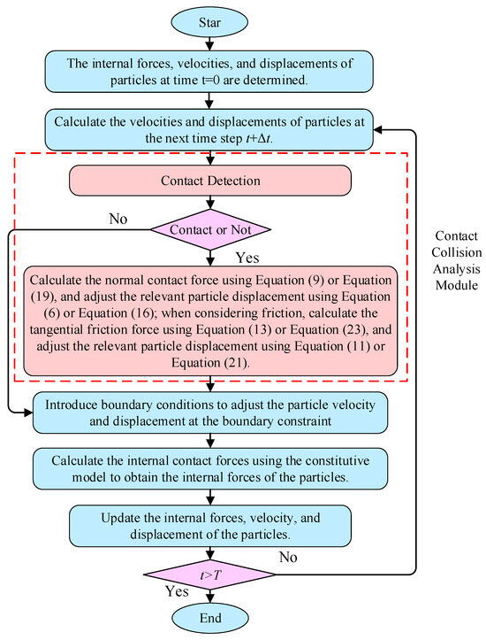
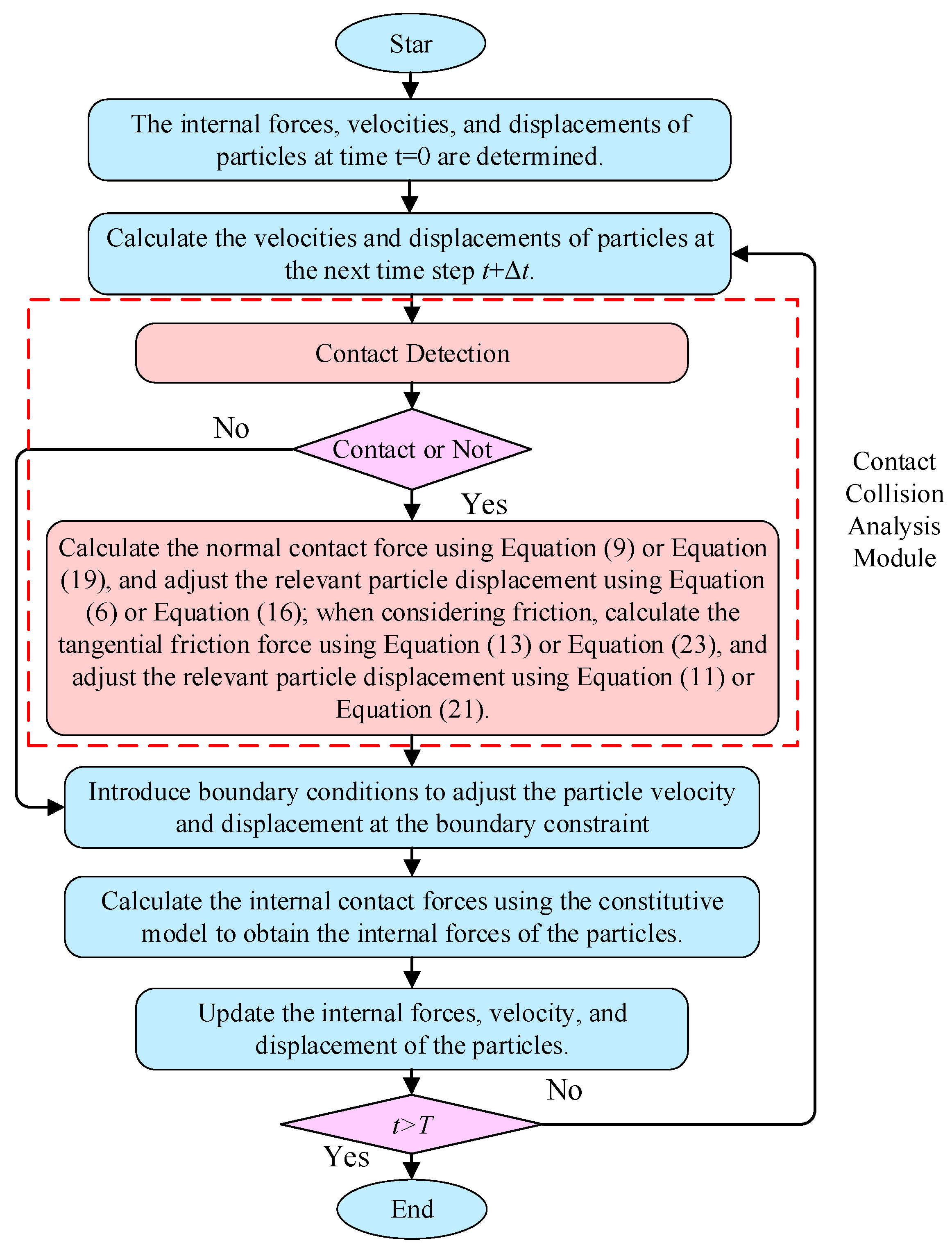
The calculation procedure for solving contact–collision problems using the MDEM is shown in Figure 7. Compared to simulations that neglect contact effects, the differences are as follows: (1) After updating the velocities and displacements of particles at the next time step, an additional contact detection procedure is introduced. This involves identifying potential contact pairs and determining whether actual contact occurs. (2) For the members that experience contact–collisions, the contact forces are calculated, and the motion equations are resolved again to push them back to the critical position. It should be noted that, within each time step, the contact force is computed using a non-iterative direct method (see Equations (9) and (19)), and thus, no convergence criterion is required. The overall time integration is performed with a fixed time step until the prescribed simulation duration is reached. As a result, the contact–collision component can be implemented as an independent computational module within the MDEM framework and activated when needed, without significantly increasing the computational complexity.

Figure 7. Flowchart of structural collision analysis using MDEM.

6. Example Analysis and Verification

6.1. Contact Between a Flexible Circular Ring and a Rigid Boundary

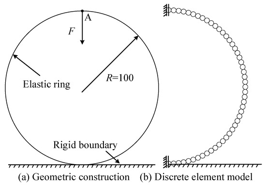
Figure 8a illustrates an example of an elastic ring subjected to a concentrated load at its top, making contact with a rigid boundary. The material parameters of the ring are: R = 100, EA = 10⁹, GA = 10⁹, and EI = 10⁴. Due to symmetry, only half of the structure was analyzed. The discrete element model is shown in Figure 8b, where the semi-ring is discretized into 49 identical spherical particles with a radius of 3.272, forming 48 contact elements. The rigid boundary was simulated using a single element. The analysis time step Δt was set to 10⁻⁴ and the contact critical threshold d₀ was set to 0.1.

Figure 8. Geometric construction and discrete element analysis models of ring.

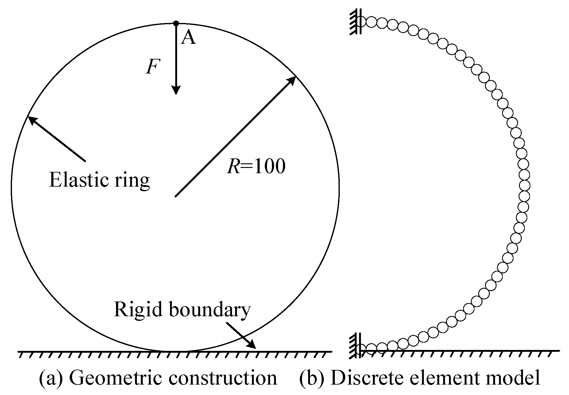
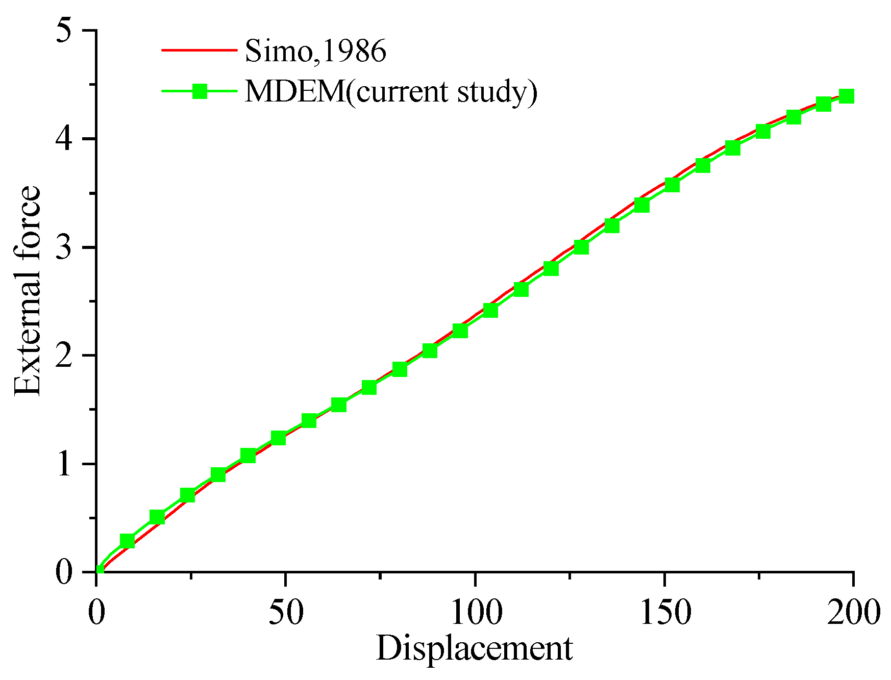
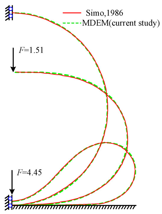
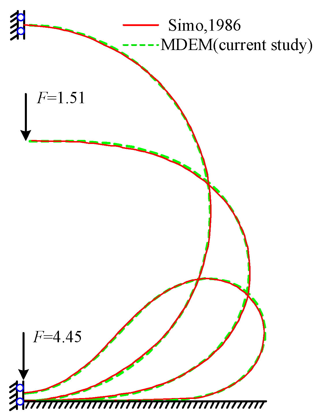
Figure 9 and Figure 10 compare the MDEM results with those from the existing literature [28]. Both the load-displacement curves and the configurations of the circular ring under different external forces were largely consistent, indicating that the contact–collision algorithm proposed in this study effectively simulates the contact behavior between the structure and the rigid boundary. As the external force increases, the contact area between the ring and the plane gradually expands.

Figure 9. Load-displacement curve of loading point A. (Data from Simo, 1986 [28]; and MDEM from the current study).

Figure 10. Deformation of the ring under different external forces. (Data from Simo, 1986 [28]; and MDEM from the current study).

6.2. Double Cantilever Beam Contact

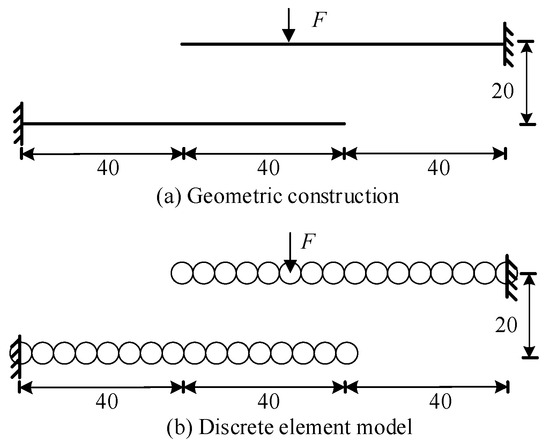
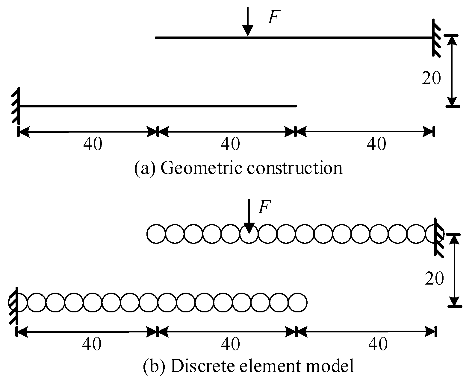
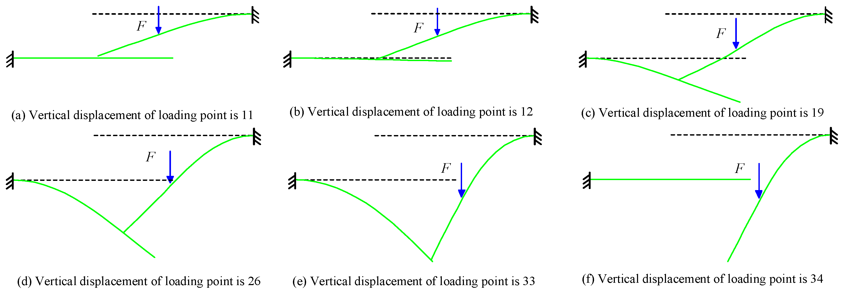
This example analyzes the contact response of a double cantilever beam. The geometric configuration of the structure is shown in Figure 11a, where EA = 10⁶, GA = 10⁶, and EI = 10⁴. Under the application of a concentrated force F, the upper cantilever beam undergoes a large deformation, and its end contacts the lower cantilever beam. Figure 11b presents the discrete element analysis model, where the structure is discretized into 32 identical spherical particles, forming 30 contact elements. A displacement loading strategy was adopted with a loading rate of 0.01. The analysis time step was set to 10⁻⁴ and a contact critical threshold d₀ was set to 0.1.

Figure 11. Double cantilever beam structure and discrete element analysis model.

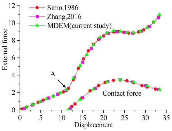
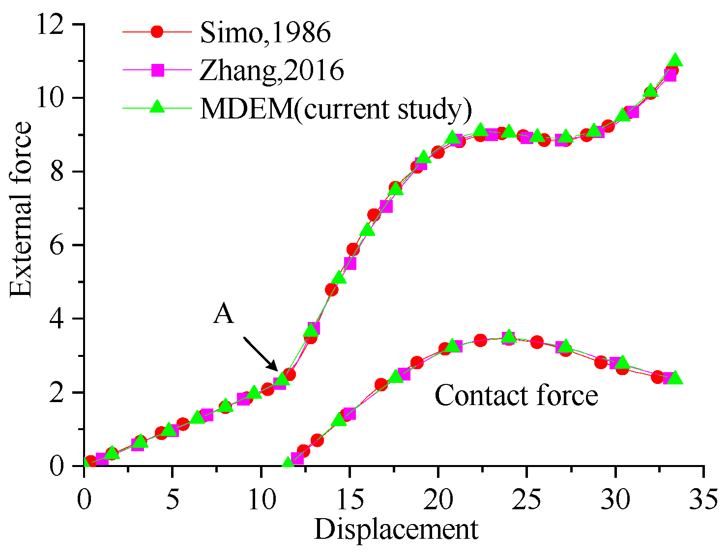
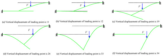
Figure 12 is the load-displacement curve at the loading point and the variation in the contact forces without considering friction effects. Combined with the deformation of the double cantilever beam in Figure 13, it can be seen that, as the external load increases, the free end of the upper cantilever beam gradually descends and makes contact with the lower cantilever beam at point A. The lower cantilever beam provides support to the upper cantilever beam, thereby enhancing the structural stiffness of the system, as evidenced by the increased slope of the load-displacement curve. After contact occurs, the end of the upper cantilever beam slides along the lower cantilever beam, with the contact point moving away from the fixed end of the lower cantilever beam. Consequently, the supporting effect of the lower cantilever beam weakens, leading to a snap-through phenomenon at the loading point, and eventually, the upper cantilever beam completely detaches from the lower cantilever beam. The obtained curve aligns well with the results from references [27,28], validating the feasibility and accuracy of the proposed method for beam–beam contact problems.

Figure 12. Load-displacement curve and total contact force of loading point. (Data from Simo, 1986 [28]; Zhang, 2016 [27]; and MDEM from the current study).

Figure 13. Contact deformation process of double cantilever beam.

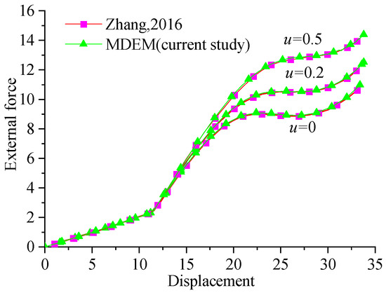
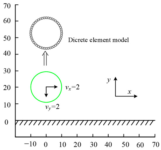
Figure 14 presents the load-displacement curves at the loading point for different friction coefficients. It can be observed that the presence of friction increases the overall stiffness of the cantilever beam system, which also rises with an increasing friction coefficient. The results obtained using the MDEM were consistent with those from the finite particle method in reference [27], thereby validating the effectiveness of the proposed contact–collision algorithm in addressing non-smooth contact problems.

Figure 14. Load-displacement curve of loading point under different friction coefficients. (Data from Zhang, 2016 [27]; and MDEM from the current study).

6.3. Collision of a Flexible Ring with a Rigid Boundary

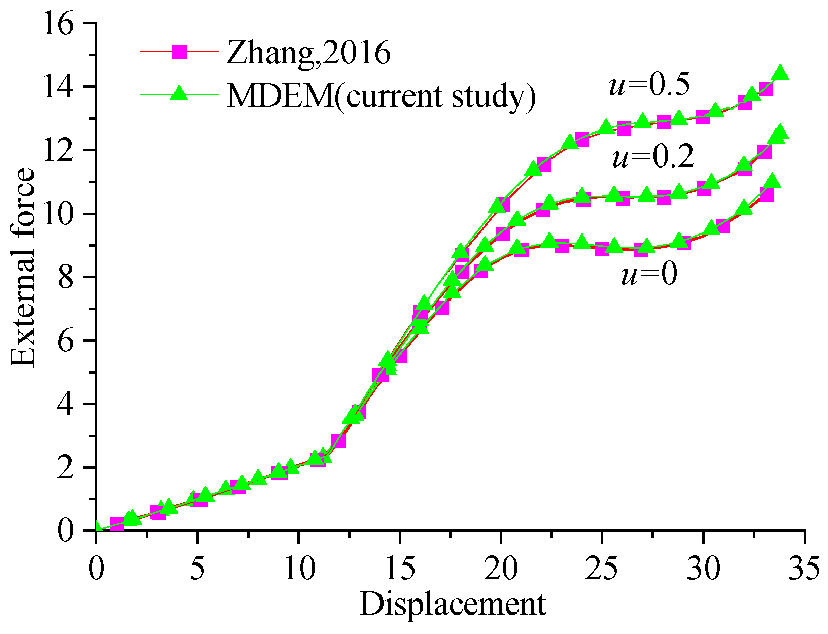
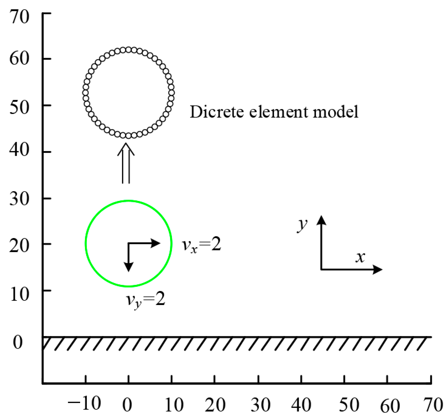
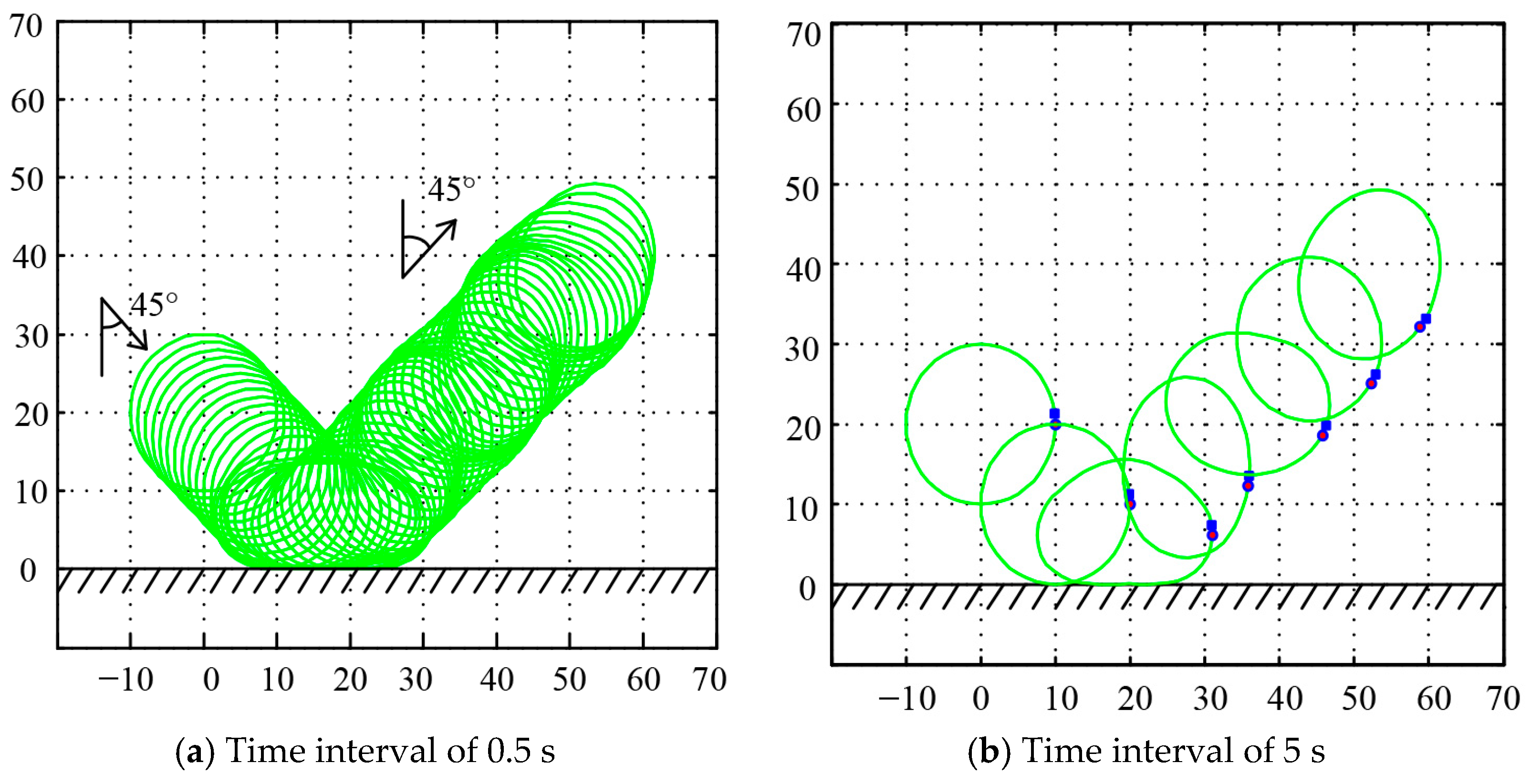
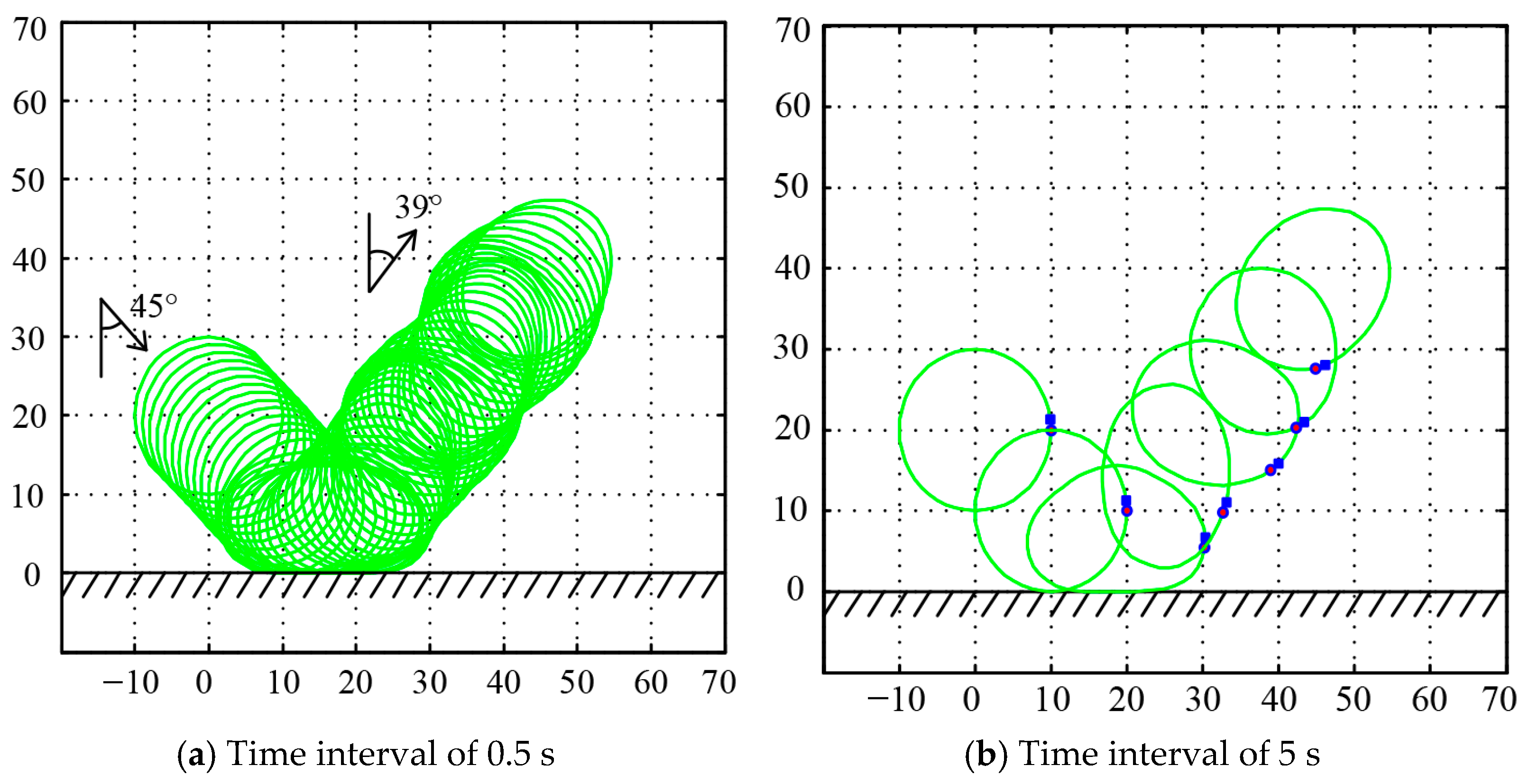
Figure 15 illustrates the contact–collision simulation of a flexible ring impacting a rigid boundary at a 45° angle. The material parameters of the ring were as follows: elastic modulus E = 100, radius R = 10, and square cross-section with a side length of 1. The density was 0.01, and damping and gravity effects were neglected. The ring was initially projected toward the rigid boundary with a speed of 2 in the positive x-direction and negative y-direction. The ring was discretized into 48 equal-sized spherical particles, forming 48 contact elements, while the rigid boundary was modeled as a single element. The analysis time step Δt was set to 1 × 10⁻⁵, and the contact critical threshold d₀ was 0.01.

Figure 15. The 45° sloping impact of a 2D ring on a rigid foundation.

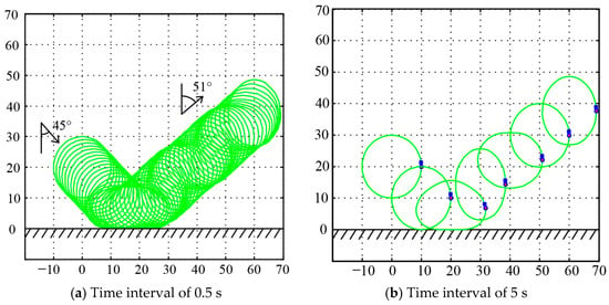
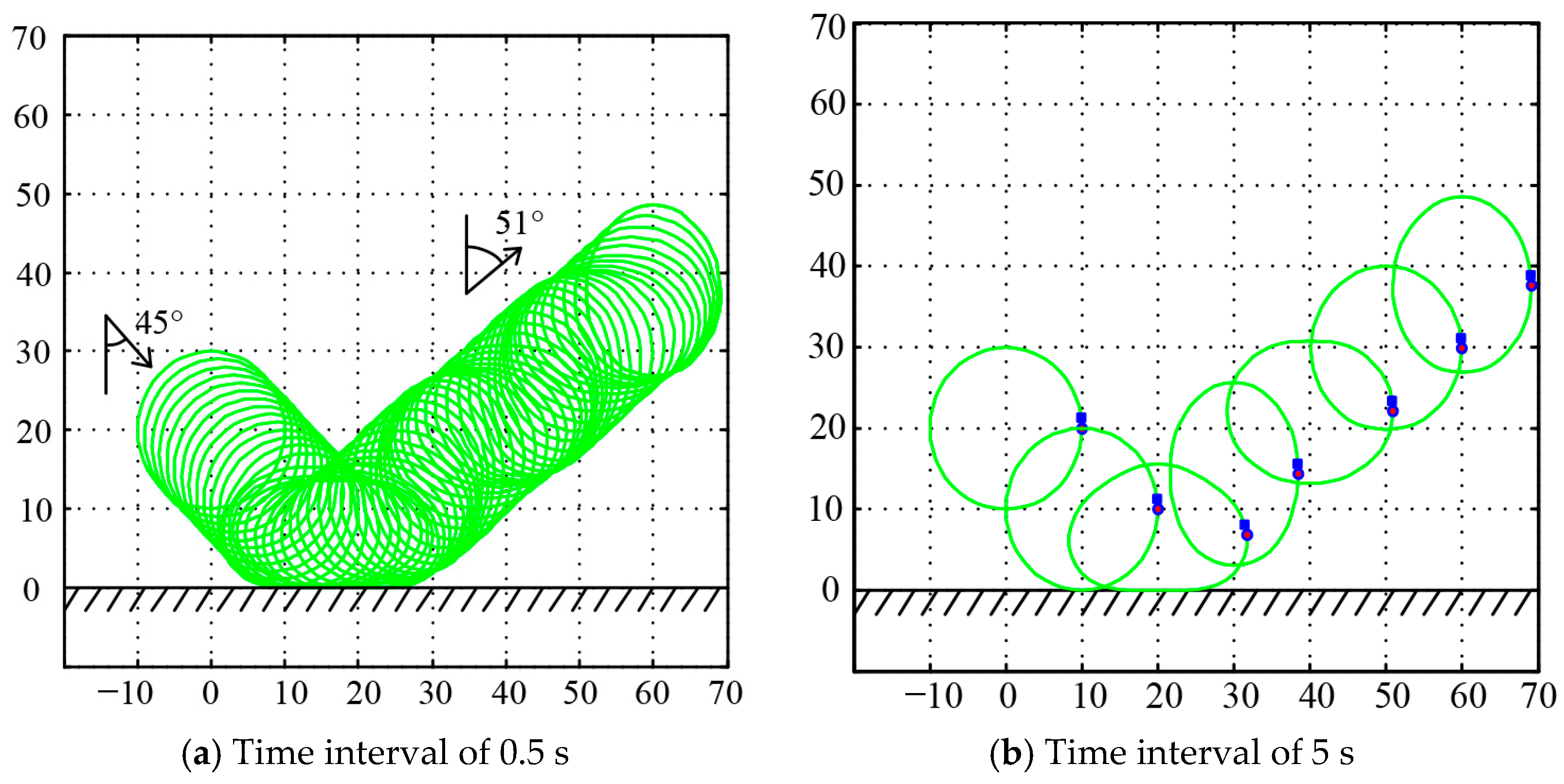
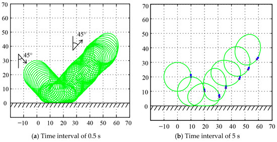
Figure 16 and Figure 17 and Figure 18 show the motion trajectories of the ring without and with the consideration of friction effects, respectively. In the absence of friction, the ring only underwent translational motion without rotation. However, when friction was considered, the induced horizontal frictional force caused the ring to rotate clockwise after the collision, with the rotational magnitude increasing proportionally to the coefficient of friction. Table 1 presents a comparison of the reflection angle and reflection velocity of the ring from MDEM simulations with those from the literature. The calculations show that, without considering friction effects, the angle between the motion direction of the rebounding ring and the y-axis was approximately 51°, which is very close to the 50° calculated by Wriggers [29] and the 50.4° calculated by Yu [30]. When the friction effect was taken into account, the friction reduced the velocity in the x-direction, resulting in a smaller angle between the rebound direction and the y-axis. Furthermore, the greater the coefficient of friction, the more the horizontal velocity is reduced after rebound, leading to a smaller angle.

Figure 16. Ring configuration change without considering friction.

Figure 17. Ring configuration change at μ = 0.1.

Figure 18. Ring configuration change at μ = 0.2.

Table 1. Reflection angle and velocity after the ring collides with the ground.

Case	Reflection Velocity	Reflection Angle/(°)
Without friction (Wriggers [29])	vx = 2; vy = 1.70	50
Without friction (Yu [30])	vx = 2; vy = 1.66	50.4
Without friction (DEM)	vx = 2; vy = 1.58	51
With friction (MDEM), μ = 0.1	vx = 1.59; vy = 1.58	45
With friction (MDEM), μ = 0.2	vx = 1.12; vy = 1.58	39

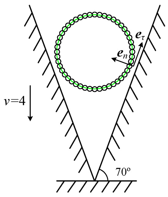
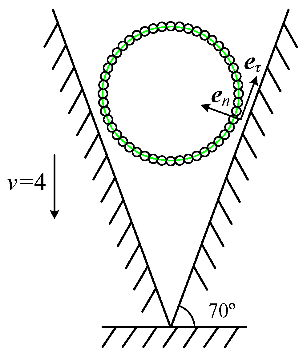
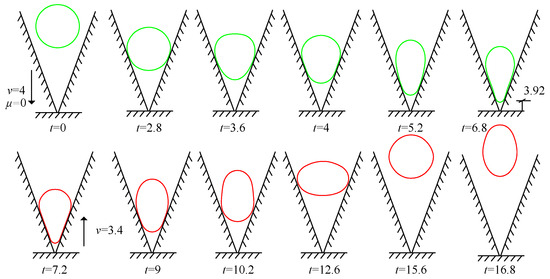
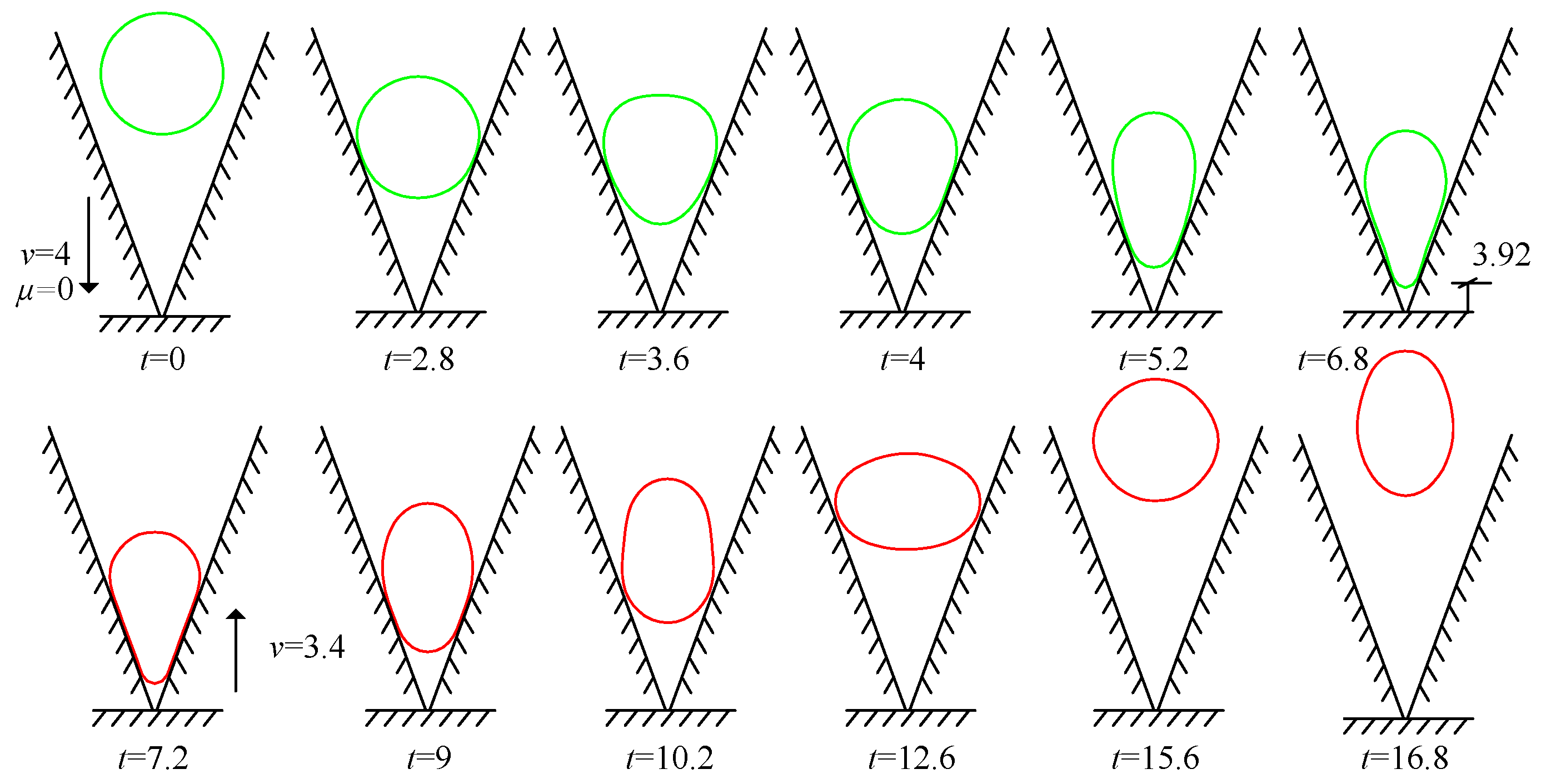
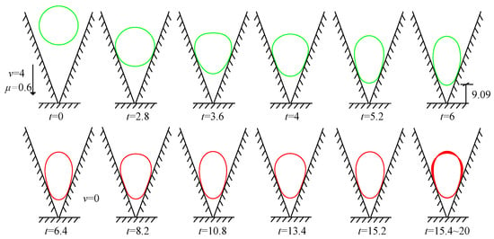
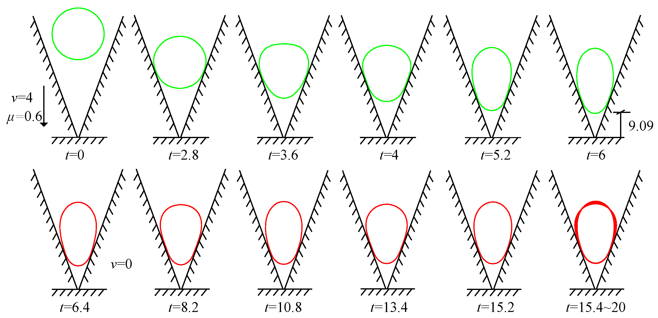
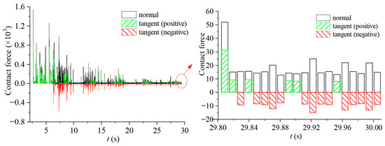
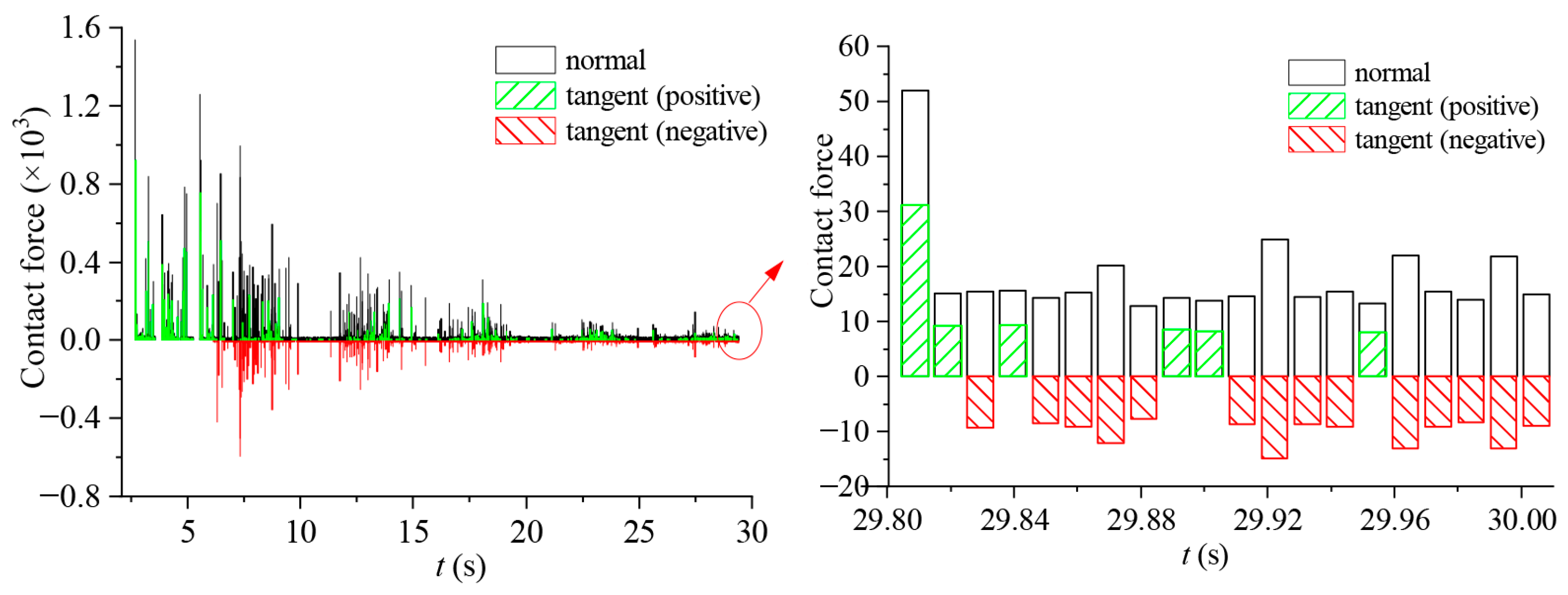
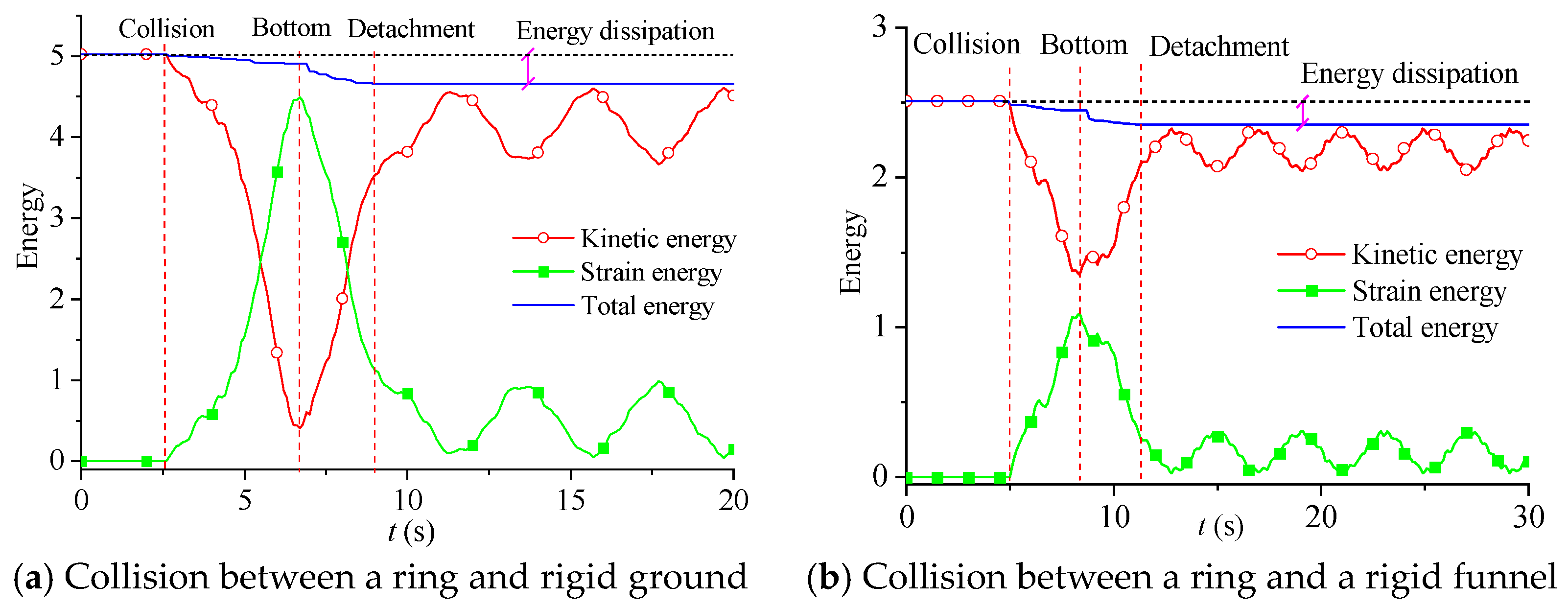
Let the aforementioned ring fall into a rigid funnel with an initial velocity of v = 4, as shown in Figure 19, while keeping the relevant analysis parameters unchanged. Each side of the funnel was modeled using a rigid element. Figure 20 shows the configuration changes of the ring without considering friction. The ring reached the bottom of the funnel at 6.8 s and subsequently detached from the funnel with a velocity of 3.4, which is relatively close to the rebound velocity of 3.1 reported in the literature [29]. When friction was considered, the ring reached the bottom of the funnel at 6 s and eventually adhered closely to the wall of the funnel, as shown in Figure 21. This phenomenon is consistent with the findings in the literature [29], primarily due to the effect of tangential friction. Figure 22 shows the time history curve of the contact force between the ring and the right-side wall of the funnel. The friction force values were mostly negative, indicating that the direction was downward along the right wall, which suppresses the rebound of the ring.

Figure 19. A model of a ring falling into a funnel.

Figure 20. Deformation of the ring falling into the rigid funnel without considering friction.

Figure 21. Deformation of the ring falling into the rigid funnel considering friction.

Figure 22. Time history of the friction force between the ring and the right wall of the funnel.

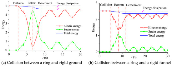
It is noteworthy that, for the free motion of the ring, the motion trend obtained using the contact simulation method proposed in this study was in good agreement with the relevant literature, although there were slight numerical differences. This was primarily due to energy dissipation during the contact and collision process; different contact simulation methods exhibit varying energy dissipation capacities due to their differing mechanisms. Figure 23 shows the energy variation for the ring without considering friction effects. It was observed that the total energy of the ring continuously decreased throughout the entire contact process with the ground or the funnel wall.

Figure 23. The energy change for the ring without considering friction.

The stability condition for the explicit time integration employed in this study is given by Δt ≤ Δt_crit = 2/ω_max, where ω_max is determined by the stiffness of the zero-length springs and the particle mass. In all the numerical examples, time steps in the range of Δt = 10⁻⁴−10⁻⁶ s were adopted, which satisfied the stability requirement.

Regarding energy behavior, the proposed method is not strictly energy-conserving. As shown in Figure 23, even in the absence of physical damping and friction, a certain degree of energy decay was observed during contact, indicating the presence of numerical damping introduced by the contact algorithm. This numerical dissipation arises from the enforcement of the non-penetration constraint through position correction, which drives the particles back to the critical configuration and does not strictly preserve the system energy. For engineering applications such as large-span structural collapse simulations, this level of numerical dissipation is generally acceptable.

6.4. Collision of Spatial Beams

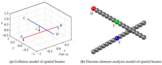
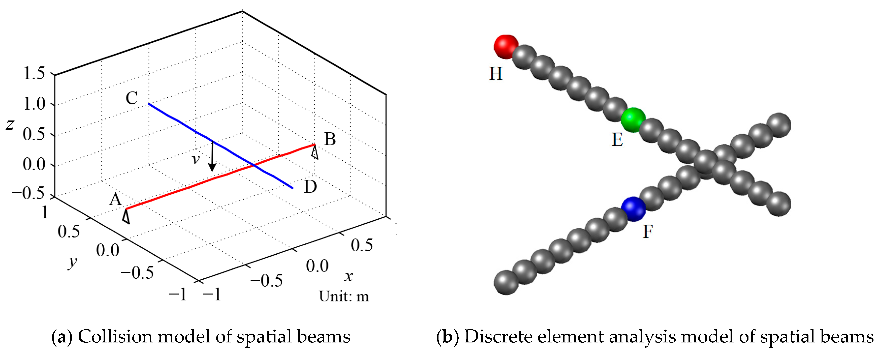
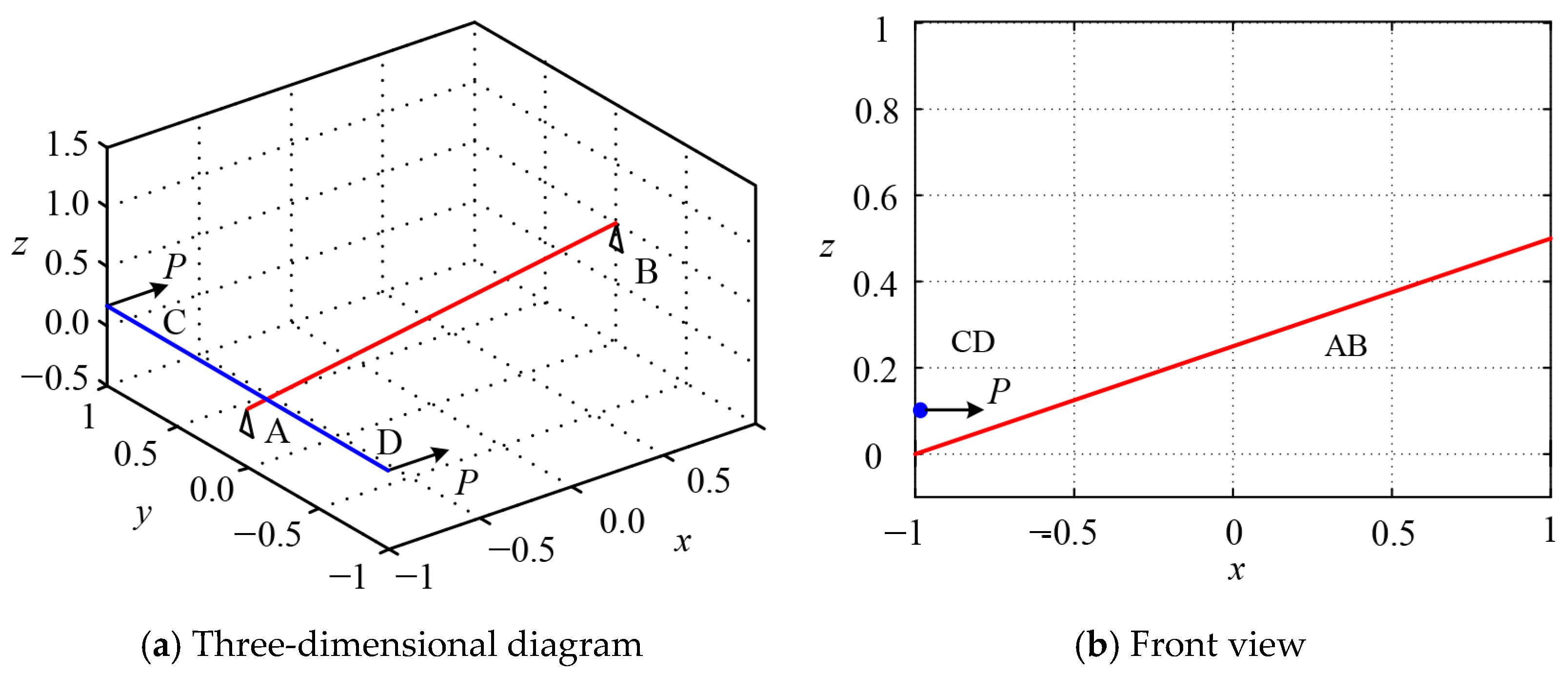
The purpose of this example was to verify the correctness of the “line–line” contact model. Figure 24 shows the spatial beams AB and CD, with the coordinates of the four nodes being (−1, 0, 0), (1, 0, 0), (0, 1, 0.5), and (0, −1, 0.5). Both ends of beam AB were hinge-constrained, while beam CD was a free spatial component moving with an initial velocity of 50 m/s along the negative z-axis. Both beams had a circular thin-walled tubular cross-section and were made of the same material: cross-sectional area A = 0.006 m², elastic modulus E = 1000 MPa, and moment of inertia I = 2.5 × 10⁻⁴ m⁴. Each beam was discretized into 16 particles, forming 30 contact elements. The analysis time step Δt was set to 1 × 10⁻⁶ s, with no consideration for damping, gravity, or friction effects, and the contact critical threshold was d₀ = 1 × 10⁻³ m.

Figure 24. Spatial beam and discrete element model.

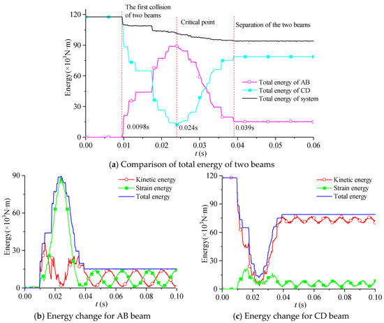
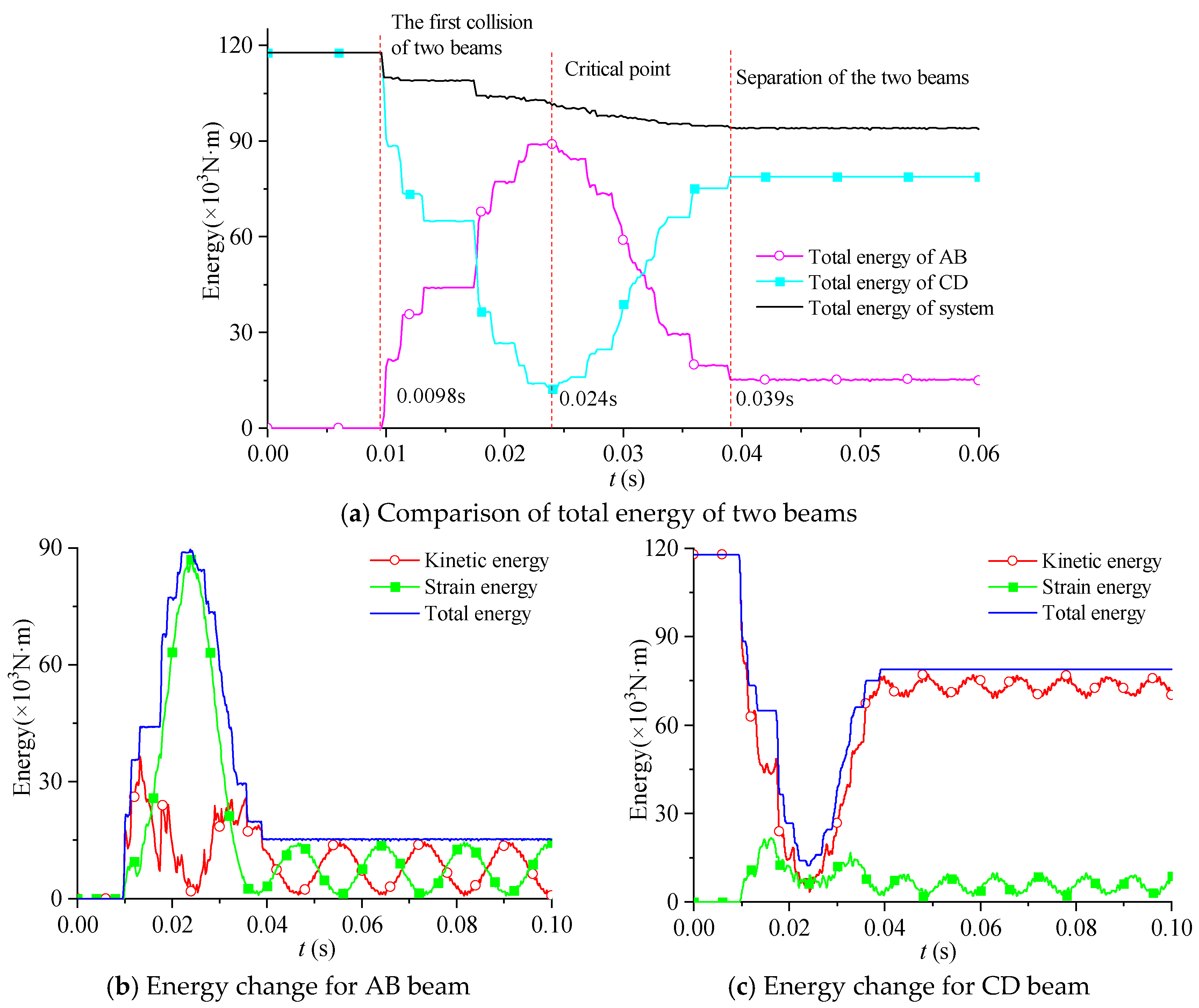
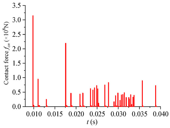
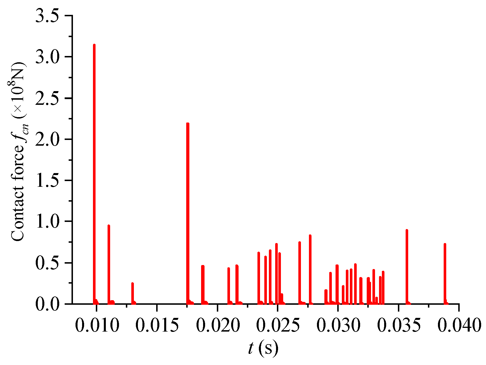
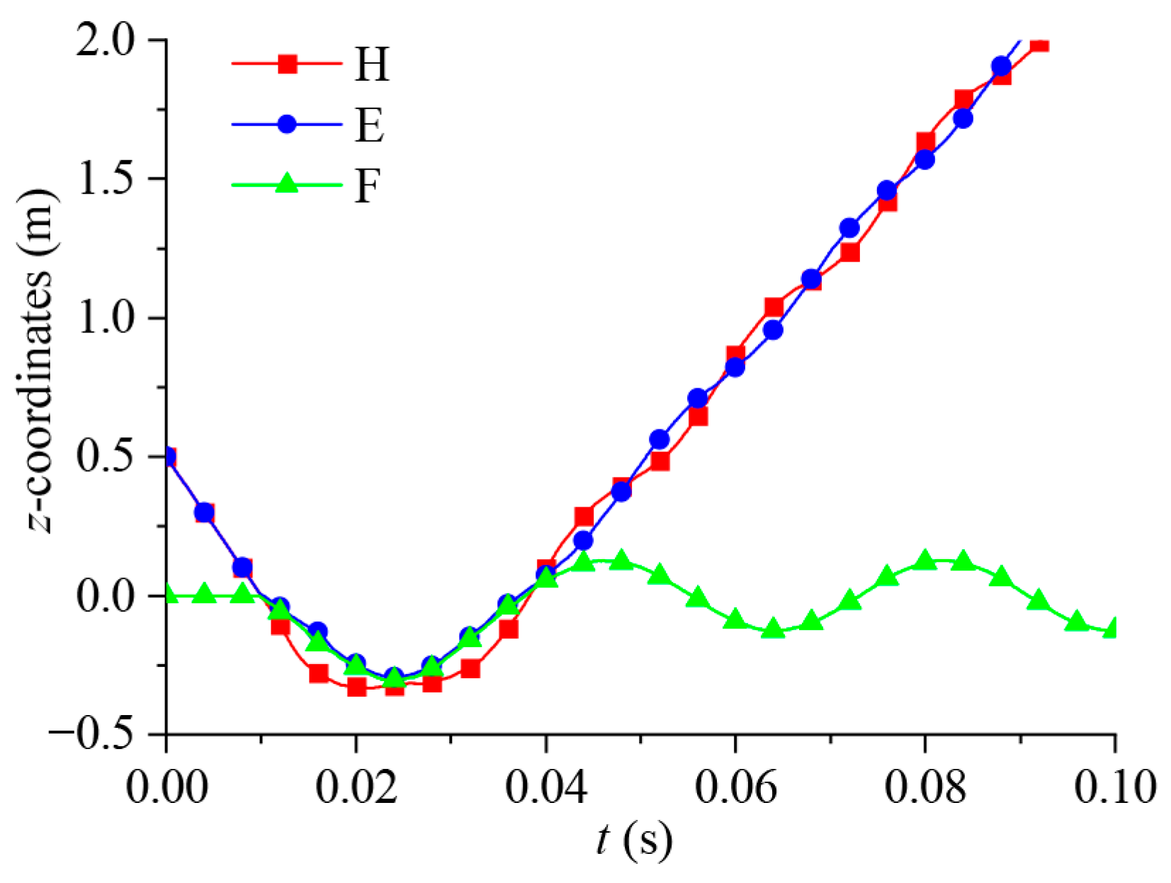
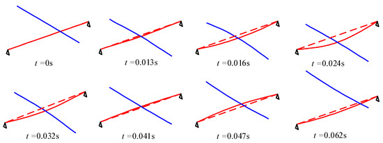
Figure 25 illustrates the energy changes for the two beams. Combining this with the time history curves of the contact force in Figure 26 and the displacement time-history curves of the recorded points in Figure 27, it can be observed that, before the collision, AB remained stationary while CD moved downward with an initial velocity. At 0.0098 s, the two components collided for the first time. Due to the impact from CD, AB was forced to move downward along with CD. At this moment, the total energy of CD (kinetic energy plus strain energy) decreased, while the total energy of AB increased. This indicates that the contact force does negative work on CD and positive work on AB. At 0.024 s, the total energy of the AB beam reached its maximum, and the total energy of CD reached its minimum, with both beams having minimal kinetic energy (see Figure 25b,c), indicating that both beams reached their lowest point (see Figure 27). Subsequently, the motion direction of AB and CD reversed, and they began to move upward. The total energy of AB continuously decreased while the total energy of CD continuously increased, indicating that the contact force does negative work on AB and positive work on CD, causing AB to rebound CD. At 0.039 s, the two beams detached, after which their respective total energies no longer changed. Since gravitational effects were neglected, CD moved upward at a velocity of 38.5 m/s, while AB underwent free vertical vibration around its original stationary position due to the hinge constraint. Figure 28 shows the configuration changes of the two rods during the collision process.

Figure 25. Energy change and comparison of two beams.

Figure 26. Contact force time history.

Figure 27. Recording point vertical displacement time history.

Figure 28. Configuration change for spatial members in the collision process.

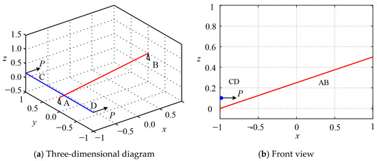
The positions of the spatial beams AB and CD were altered, as shown in Figure 29, with the coordinates of the four nodes being (−1, 0, 0), (1, 0, 0.5), (−1, 1, 0.1), and (−1, −1, 0.1). The ends of the CD beam were subjected to a horizontal concentrated force P acting in the positive x-direction. All the analysis parameters remained unchanged except for the friction. A displacement loading strategy was employed in the MDEM analysis, with a loading rate of 0.001 m/s.

Figure 29. Schematic diagram of the position of the space beam (unit: m).

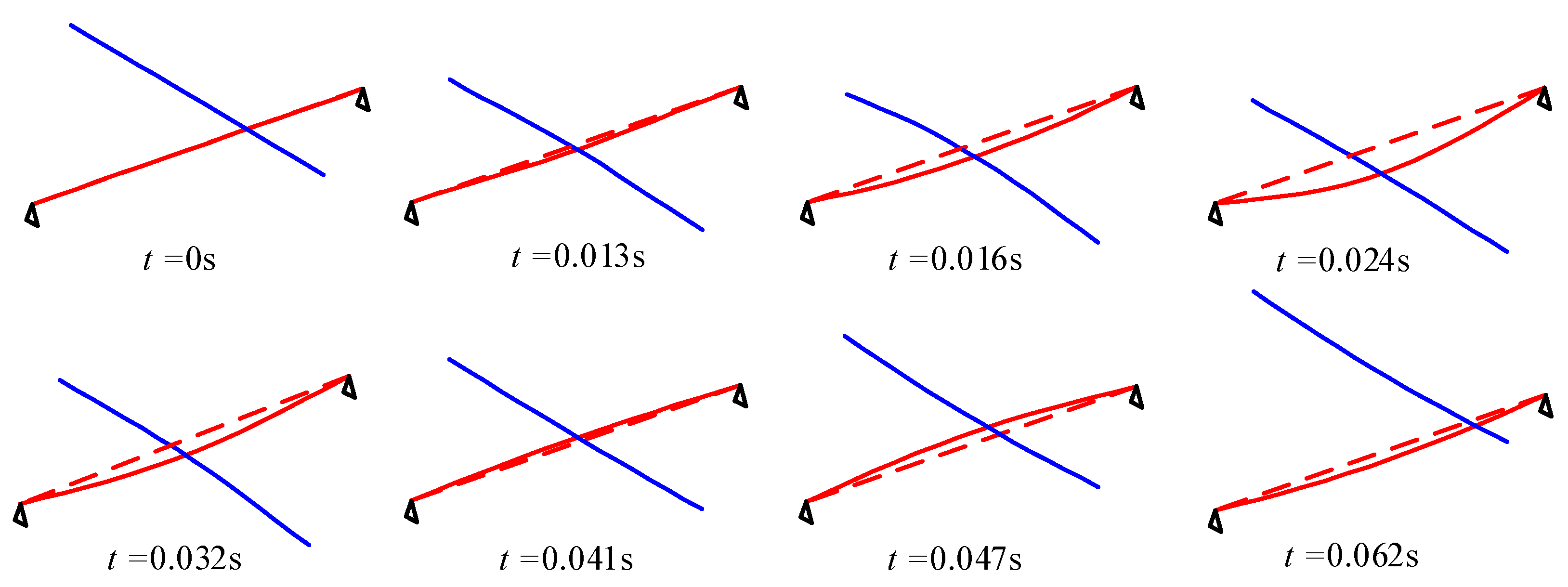
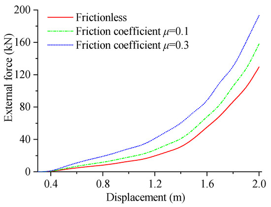
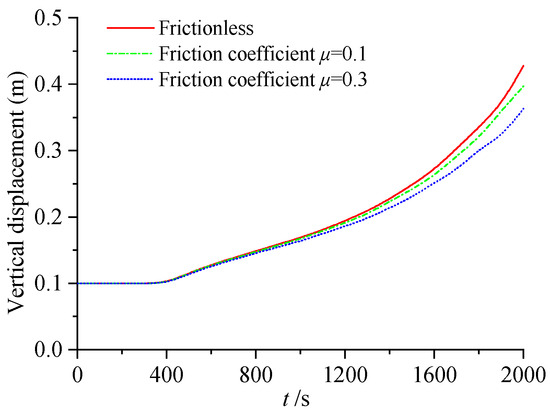
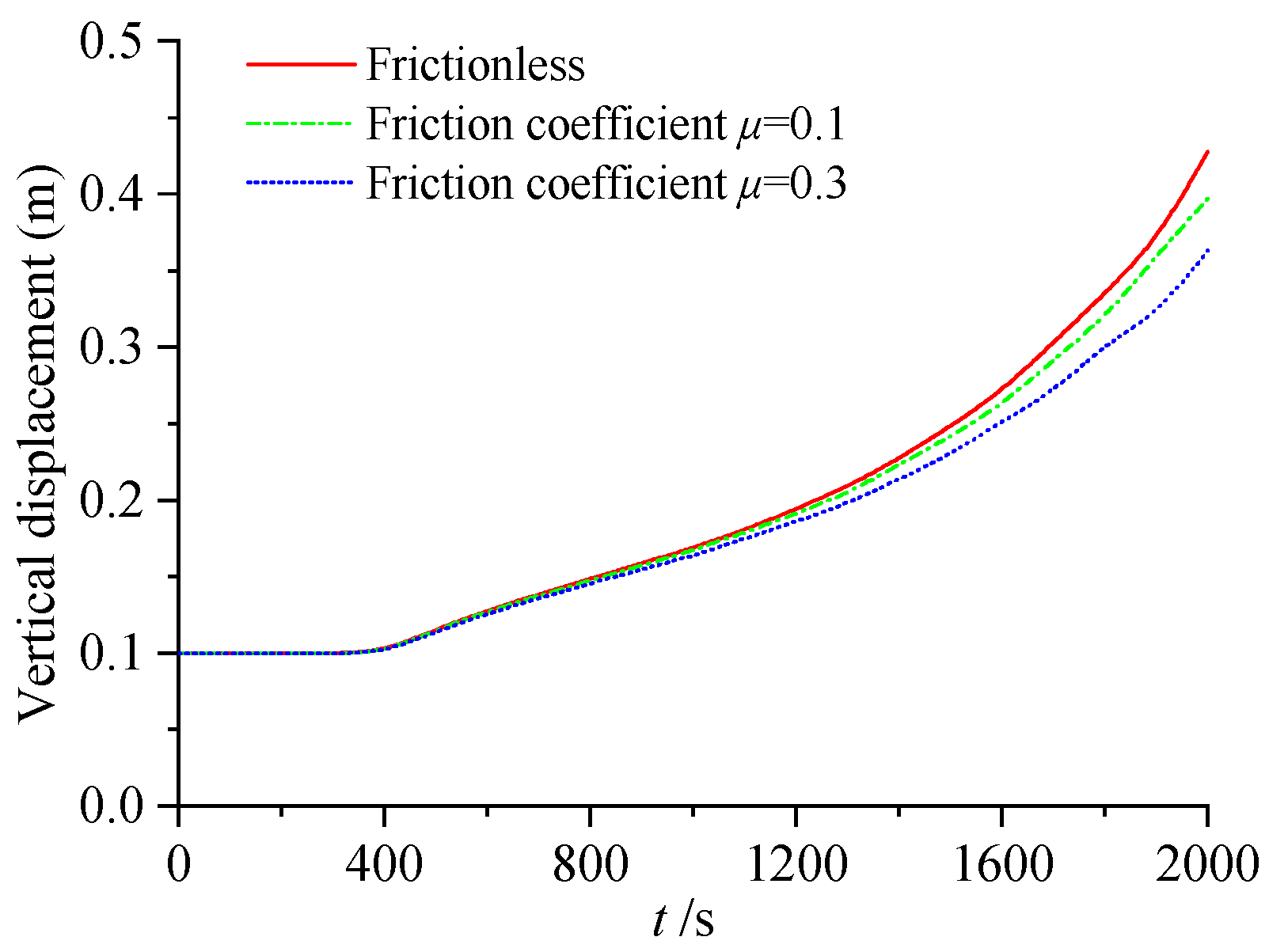
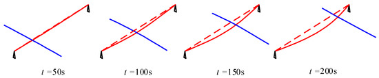
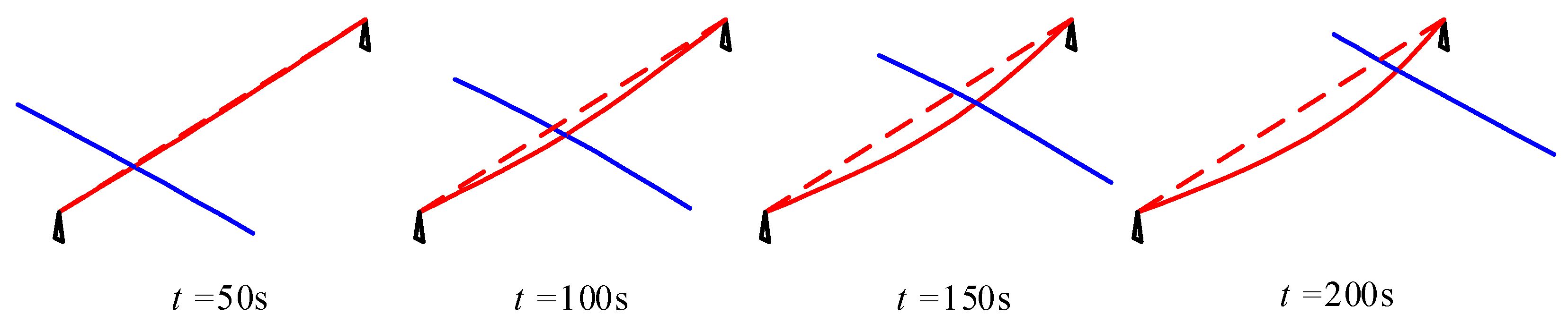
Figure 30 shows the load-displacement curve at loading point C. It was observed that, when beam CD moved 0.4 m in the positive x-direction, it made contact with beam AB and was supported by it. The curvature of the curve increased, and this value grew with the increasing friction coefficient. Figure 31 presents the time history curve of the vertical displacement of particle E (as shown in Figure 24b). It can be seen that, after beam CD contacted beam AB, particle E slid upward along beam AB. When considering the effect of friction, the generated frictional force impeded the upward movement of particle E, and the greater the friction coefficient, the larger the resistance. Consequently, the vertical displacement that occurred at the same moment was smaller. Figure 32 illustrates the contact deformation process of the two beams without considering friction.

Figure 30. Load-displacement curve of loading point C.

Figure 31. Vertical displacement time history of recording point E.

Figure 32. Contact deformation process of space beams without considering friction.

The numerical results obtained using the proposed method showed good agreement with the FEM and finite particle method results reported in the literature, thereby validating its accuracy and effectiveness.

7. Discussion

7.1. Novelty and Contributions

The main contributions of this study are reflected in the following aspects:

(1)

Point–line and line–line contact models were established within the MDEM framework, providing a unified approach for member-level collision analyses.

(2)

The concept of virtual contact point pairs was introduced, and closed-form solutions of the non-penetration constraints were derived (see Equations (9) and (19)), eliminating the need for iterative calculation of contact forces.

(3)

A modular contact–collision subroutine was developed, which can be invoked independently without affecting the fundamental analysis procedure of the MDEM.

7.2. Advantages of the Proposed Method

The proposed method offers several advantages. First, it avoids the reconstruction of global stiffness matrices, making it well suited for explicit dynamic analyses. Second, contact forces are obtained directly through closed-form solutions based on non-penetration constraints, eliminating iterative procedures. Third, the unified treatment of “point–line” and “line–line” contact modes simplifies the modeling process. These features make the method efficient and suitable for collapse simulations involving complex contact interactions.

7.3. Limitations

The proposed method has the following limitations:

(1)

Zero-length spring assumption: Although validated in previous studies, this simplification may introduce artificial stiffness in bending-dominated problems when the discretization is insufficient. It is recommended to use at least eight particles per member to maintain an acceptable accuracy.

(2)

Friction modeling: The current model assumes identical static and kinetic friction coefficients and does not account for velocity-dependent effects (e.g., the Stribeck effect). For the impact-dominated problems considered here, this simplification had a minor influence on the overall structural response.

(3)

Contact detection: A global search was used without acceleration structures (e.g., spatial hashing or KD-trees). This approach was computationally feasible for the problem scale considered (~50 particles), but may become inefficient for large-scale engineering applications.

(4)

Validation: Numerical examples were primarily compared with results from the literature (e.g., the FEM and finite particle methods). Direct experimental validation and real large-span engineering case studies are currently lacking.

7.4. Scope of Applicability

The proposed method is applicable to contact–collision analyses of member-based structures, particularly for large-span structures (e.g., reticulated shells and trusses) undergoing collapse, where geometric nonlinearity is significant and contact interactions are frequent. For problems with small deformations and limited contact, conventional finite element methods may offer a higher computational efficiency.

7.5. Future Work

Future research directions include the following aspects:

(1)

Introducing acceleration structures such as spatial hashing or KD-trees to improve the efficiency of contact detection.

(2)

Extending the proposed method to collapse simulations of real large-span engineering structures (e.g., stadiums and airport terminals).

(3)

Incorporating velocity-dependent friction models and friction regularization techniques.

(4)

Developing a GPU-parallelized implementation to enhance the computational efficiency.

(5)

Conducting experimental validation to further verify the reliability of the proposed method.

8. Conclusions

This study presents a unified contact modeling approach within the MDEM framework for simulating collision behavior in member systems.

The proposed method establishes a consistent framework for handling both “point–line” and “line–line” contact modes and introduces a virtual contact point pair concept to derive closed-form contact force solutions. Numerical examples demonstrated that the method achieves a good accuracy while avoiding global stiffness matrix reconstruction.

The results indicate that the proposed approach provides an efficient and practical tool for simulating contact–collision behavior in large-span structural collapse, with potential applications in engineering analyses and structural design.

In terms of future development, the proposed method can be extended to large-scale engineering applications involving complex contact–collision interactions. With the incorporation of efficient contact search algorithms and advanced constitutive models, it can be integrated into numerical tools for collapse analyses, safety assessments, and risk evaluations of large-span structural systems.

References

- Hughes, T.J.; Taylor, R.L.; Sackman, J.L.; Curnier, A.; Kanoknukulchai, W. A finite element method for a class of contact-impact problems. Comput. Methods Appl. Mech. Eng. 1976, 8, 249–276. [Google Scholar] [CrossRef] [Scilit]
- Chaudhary, A.B.; Bathe, K.J. A solution method for static and dynamic analysis of three-dimensional contact problems with friction. Comput. Struct. 1986, 6, 855–873. [Google Scholar] [CrossRef] [Scilit]
- Oden, J.T.; Kikuchi, N. Finite element methods for constrained problems in elasticity. Int. J. Numer. Methods Eng. 1982, 18, 701–725. [Google Scholar] [CrossRef] [Scilit]
- Papadopoulos, P.; Taylor, R.L. A mixed formulation for the finite element solution of contact problems. Comput. Methods Appl. Mech. Eng. 1992, 94, 373–389. [Google Scholar] [CrossRef] [Scilit]
- Zhong, Z.H.; Nilsson, L. Lagrange multiplier approach for evaluation of friction in explicit finite-element analysis. Commun. Numer. Methods Eng. 1994, 10, 249–255. [Google Scholar] [CrossRef] [Scilit]
- Qi, N.; Ye, J.H. Geometric nonlinear analysis with large deformation of member structures by discrete element method. J. Southeast Univ. Nat. Sci. Ed. 2013, 43, 917–922. (In Chinese) [Google Scholar]
- Qi, N.; Ye, J.H. Application of elastic discrete element method in member structures. Eng. Mech. 2017, 34, 11–20. (In Chinese) [Google Scholar]
- Xu, Q.; Ye, J. An adaptively coupled DEM–FEM algorithm for geometrical large deformation analysis of member structures. Comput. Part. Mech. 2020, 7, 947–959. [Google Scholar] [CrossRef] [Scilit]
- Qi, N.; Ye, J.H. Application of discrete element method in member structures: Elestoplastic analysis. J. Vib. Eng. 2017, 30, 929–937. (In Chinese) [Google Scholar]
- Ye, J.H.; Zhang, M. Discrete element method for elastoplastic buckling analysis of single-layer reticulated shells. Eng. Mech. 2019, 36, 30–37. (In Chinese) [Google Scholar]
- Ye, J.; Xu, L. Member Discrete Element Method for Static and Dynamic Responses Analysis of Steel Frames with Semi-Rigid Joints. Appl. Sci. 2017, 7, 714. [Google Scholar] [CrossRef] [Scilit]
- Ye, J.H.; Xu, Q. Study on numerical calculation method of semi-rigid connections based on member discrete element theory. J. Build. Struct. 2022, 43, 311–321. [Google Scholar]
- Xu, L.L.; Ye, J.H. Application and error improvement of large mass method used in DEM-based multi-support excitation analysis. China Civ. Eng. J. 2016, 49, 32–36. (In Chinese) [Google Scholar]
- Qi, N.; Ye, J.H. Nonlinear Dynamic Analysis of Space Frame Structures by Discrete Element Method. Appl. Mech. Mater. 2014, 638–640, 1716–1719. [Google Scholar]
- Xu, L.L.; Ye, J.H. Study on the calculation theory of member discrete element for static and dynamic elastoplastic analysis. Eng. Mech. 2021, 38, 1–11. (In Chinese) [Google Scholar]
- Ye, J.H.; Zhang, M. Buckling behavior of single-layer reticulated shells based on member discrete element method. J. Build. Struct. 2019, 40, 54–61. (In Chinese) [Google Scholar]
- Ye, J.; Qi, N. Collapse process simulation of reticulated shells based on coupled DEM/FEM model. J. Build. Struct. 2017, 38, 52–61. (In Chinese) [Google Scholar]
- Jihong, Y.; Nian, Q. Combination of DEM_FEM for Progressive Collapse Simulation of Domes Under Earthquake Action. Int. J. Steel Struct. 2018, 18, 305–316. [Google Scholar] [CrossRef] [Scilit]
- Xu, L.; Ye, J. DEM Algorithm for Progressive Collapse Simulation of Single Layer Reticulated Domes under Multi Support Excitation. J. Earthq. Eng. 2019, 23, 18–45. [Google Scholar] [CrossRef] [Scilit]
- Jihong, Y.; Nian, Q. Progressive collapse simulation based on DEM for single-layer reticulated domes. J. Constr. Steel Res. 2017, 128, 721–731. [Google Scholar] [CrossRef] [Scilit]
- Cai, W.; Gao, K.; Ai, S.G.; Qiao, Y. A 2D Unified Distance Potential Field-Based Contact Interaction Algorithm for Combined Finite-Discrete Element Method (FDEM). Rock Mech. Rock Eng. 2025, 58, 6869–6892. [Google Scholar] [CrossRef] [Scilit]
- Zhang, P.; Ren, S.; Fu, C.; Cheng, C.; Galindo-Torres, S.A.; Lan, R. Improved Metaball Discrete Element Method with Robust Contact Algorithm for General-Shaped Particles with Rounded Features. Appl. Sci. 2025, 15, 12561. [Google Scholar] [CrossRef] [Scilit]
- Liu, M. A contact detection algorithm for polyhedrons based on improved common-plane concept. Sci. Rep. 2025, 15, 39922. [Google Scholar] [CrossRef] [Scilit]
- Neto, A.G.; Wriggers, P. Discrete element model for general polyhedra. Comput. Part. Mech. 2022, 9, 353–380. [Google Scholar] [CrossRef] [Scilit]
- Liu, G.Y.; Xu, W.J.; Zhou, Q.; Zhang, X.L. The polyhedron overlap algorithm based on the blocky discrete element method. Chin. J. Comput. Mech. 2022, 39, 265–272. [Google Scholar]
- Dong, Y.J.; Pan, X.Y.; Yang, X.X. A calculation method for finding the foot of common perpendicular of lines on different places. J. Harbin Univ. Sci. Tech. 1990, 14, 84–88. [Google Scholar]
- Zhang, P.F. Research on Numerical Methods for Structural Failure Simulation. Ph.D. Thesis, Zhejiang University, Hangzhou, China, 2016. [Google Scholar]
- Simo, J.C.; Wriggers, P.; Schweizerhof, K.H.; Taylor, R.L. Finite deformation post-buckling analysis involving inelasticity and contact constraints. Int. J. Numer. Methods Eng. 1986, 23, 779–800. [Google Scholar] [CrossRef] [Scilit]
- Wriggers, P.; Van, T.V.; Stein, E. Finite element formulation of large deformation impact-contact problems with friction. Comput. Struct. 1990, 37, 319–331. [Google Scholar] [CrossRef] [Scilit]
- Yu, Y.; Luo, Y.Z. Impact analysis of structures based on finite particle method. Eng. Mech. 2013, 30, 66–77. [Google Scholar]
Disclaimer/Publisher’s Note: The statements, opinions and data contained in all publications are solely those of the individual author(s) and contributor(s) and not of MDPI and/or the editor(s). MDPI and/or the editor(s) disclaim responsibility for any injury to people or property resulting from any ideas, methods, instructions or products referred to in the content. |
© 2026 by the authors. Licensee MDPI, Basel, Switzerland. This article is an open access article distributed under the terms and conditions of the Creative Commons Attribution (CC BY) license.