Nonlinear Behavior and Dynamic Properties of Cohesive Soil Under Seismic Cyclic Loading Considering Strain History Effects

Abstract

In earthquake engineering and hydraulic engineering, the dynamic mechanical behavior of cohesive soils is crucial to ensure structural stability. However, most existing dynamic constitutive models fail to adequately account for the influence of strain history, which is essential for accurately predicting soil behavior under seismic loading. This study conducted a series of cyclic single-shear tests on both in situ and disturbed Changsha cohesive soils. Hysteresis curves were obtained under varying shear strain amplitudes to investigate the degradation patterns of the dynamic shear modulus and the evolution of the damping ratio. Furthermore, multi-cycle loading tests under constant strain amplitude were carried out to clarify the correlation between damping ratio, dynamic shear modulus, and the number of loading cycles. A simplified practical dynamic model, applicable to general cohesive soils, is proposed. This model incorporates the effect of strain history and provides a valuable reference for analyzing the dynamic response of soils subjected to earthquake actions.

1. Introduction

In earthquake engineering, hydraulic engineering, and slope engineering, the stability of buildings depends heavily on the mechanical characteristics of the soil. A large number of engineering practices show that the soil’s mechanical characteristics change under complex stress [1,2,3], which causes destabilization of underground tunnels, slopes, or above-ground structures [4,5,6]. For this reason, it is crucial to complete a study on the behavior of soil under dynamic loading to clarify the disaster-causing mechanism of geotechnical structures [7,8].

In general, the dynamic properties of soils are usually characterized by soil stiffness and damping. Therefore, dynamic tests on soil samples are usually carried out at the laboratory scale to obtain the soil hysteresis curve, which in turn, can be used to obtain the law of fluctuation of the damping ratio to the dynamic shearing modulus with shear strain [9,10,11]. Owing to the inherent anisotropy of soil, the dynamic stress–strain relationship exhibits three characteristic features: nonlinearity, hysteresis, and cumulative deformation. Zhang [12] et al. used centrifugal test data to investigate the ability of the boundary plane plasticity model to match the multiaxial dynamic hysteresis response of soil sediments under broadband (e.g., seismic) excitation, and the results showed that the model proposed by Borja and Amies [13] was able to forecast the soil dynamic hysteresis response under seismic inputs. Taborda [14] et al. described a new relationship of soil unloading/reloading behavior under cyclic loading by applying the hill-climbing technique and evaluated the performance of the proposed model. Thomas [15] et al. solved the extended critical state elastic–plasticity constitutive model based on the net stress and suction by using the finite element technique. Feng et al. [16] developed the intrinsic relationship of soil using data from a consolidated drainage test by using the soft soil test in Jiading District, Shanghai, China, and verified the constitutive model of the soft soil. Lu et al. [17] utilized data from a geotechnical tri-axial test on desert soil to introduce quantitative structural parameters of the soil into the analysis of the properties of soil deformation and strength, and established a constitutive relationship for sandy soil using the Duncan–Zhang model. Chen et al. [18] defined new structural parameters for in situ loess in stress–strain curves at different water contents, which were normalized to structural stress–strain curves. Jun et al. [19] proposed representative equations for the constitutive relationship of soft soils dredged and reclaimed in Korea by means of marine soft soil laboratory tests. Zhou et al. [20] carried out a number of tri-axial tests on residual soils in Guangdong Province and obtained coefficients of stress–strain functions. All of the above studies were fitted for specific soil materials using existing soil constitutive models. The research on dynamic constitutive models has primarily focused on soft soils in coastal areas or loess in the northwest, while relatively little attention has been paid to the cohesive soils widely distributed in the central and southern regions (such as those in Hunan). Although these soils possess unique geological origins and structural characteristics, their dynamic response patterns under seismic loading remain unclear, and studies on their dynamic properties that account for the effects of strain history are particularly scarce.

Soil may be subjected to cyclic cumulative loads in practical engineering, and the internal rearrangement of the soil may occur under cyclic loads, which may accordingly change the mechanical behavior of the soil. Cui et al. [21] explored the stacking behavior of coarse-grained soils under different initial static stresses through a sequence of triaxial cyclic tests, and showed that, under the same cyclic load, the higher the initial stress ratio or the lower the circumferential pressure of the specimen, and the more cumulative axial strain that can be detected, the more accumulated axial strain. Xu [22], based on the three-limit equilibrium theory, proposed a calculation method for the strength parameters of soil–rock materials under three-dimensional conditions, and by using this method, the residual strength parameters, as well as the soil–rock strength parameters, in the study area were obtained. Zhang et al. [23], using the critical state soil mechanics framework (CSSM) theory, established the correlation between the interfacial state parameter and the friction angle in different interfacial states. Rui et al. [24] analyzed the mechanical behavior of three kinds of soil samples under cyclic traffic loading, including unstable, sub-stable, and stable cases, using a hollow cylinder device, and proposed a new approach to elucidate the stability of soils under cyclic stress ratios at different frequencies. Zapata [25] investigated the effect of the stress history of the natural soil deposit during reconsolidation on the subsequent behavior of severely over-consolidated clays under monotonous and cyclic loading. Pedroso [26] et al. proposed an unsaturated dynamic constitutive relationship for unsaturated clayey soils, related to the previously expanded BBM elastic-plastic model. Yang et al. [27,28] constructed a dynamic elastic–plastic constitutive model for unsaturated structural loess under cyclic loading using an elastic–plastic model, cementum damage law, and unsaturated soil mechanics.

In summary, models for the dynamic constitutive analysis of soil considering strain history under cyclic loading are less studied. In particular, Changsha cohesive soil, widely distributed in residual hills and gullies in southern China, is commonly used as a foundation-bearing layer. Despite its engineering relevance, its dynamic behavior under seismic loading remains underexplored. While previous studies have focused on monotonic or small-strain behavior, few have addressed the cumulative effects of strain history under cyclic loading. This study bridges that gap by combining multi-amplitude cyclic tests with a model that incorporates volumetric strain accumulation.

In this paper, firstly, cyclic single-shear tests were conducted on cohesive in situ and disturbed soils at the laboratory scale to obtain hysteresis curves of soils under different strain amplitudes, and to clarify the law of dynamic shear modulus variation, as well as the damping ratio, with shear strain. Then, the parameter sensitivity of nonlinear dynamic models of soils containing multiple parameters was analyzed, and expressions for the dynamic shear modulus and damping ratio of the Changsha soils were obtained at different shear strains. Furthermore, the correlation between the damping ratio and dynamic shear modulus of Changsha clayey soil with respect to the number of cyclic loadings was obtained by using multiple cyclic loading under a single strain amplitude, and a simple and practical dynamic characterization model for ordinary cohesive soils that can consider the effect of strain history was proposed, which can provide guidance for the analysis of the dynamic response of soils in water conservancy projects and slope projects under the effect of earthquakes.

2. Methodology

2.1. Research Framework

This study investigates the nonlinear mechanical behavior of Changsha cohesive soils under seismic cyclic loading through a systematic experimental and analytical approach. The research methodology comprises three primary components: (1) physical characterization of in situ and disturbed cohesive soil samples from Changsha, China; (2) cyclic single-shear tests to obtain hysteresis curves across multiple strain amplitudes; and (3) development and validation of a three-parameter Davidenkov constitutive model incorporating strain history effects. The model enables the quantification of cumulative volumetric strain effects on the dynamic shear modulus and damping ratio.

2.2. Soil Sampling and Preparation

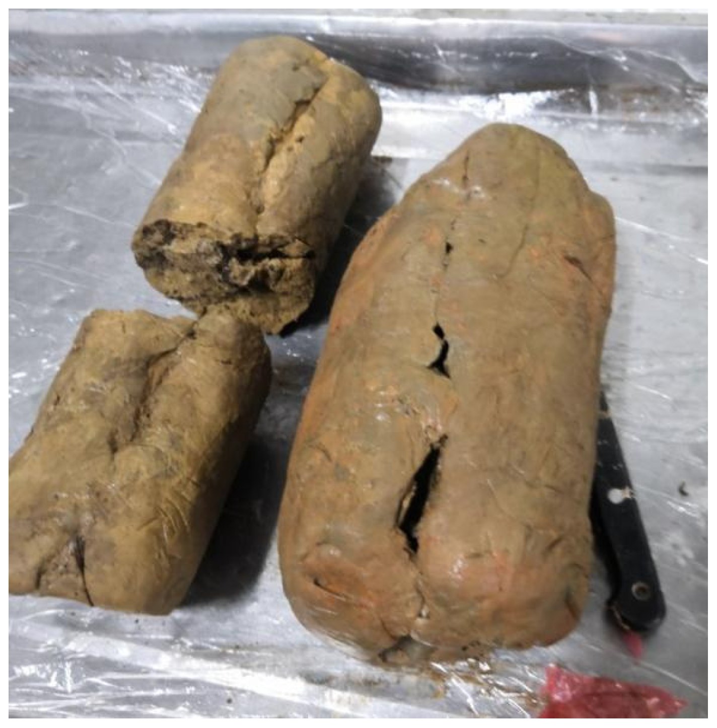
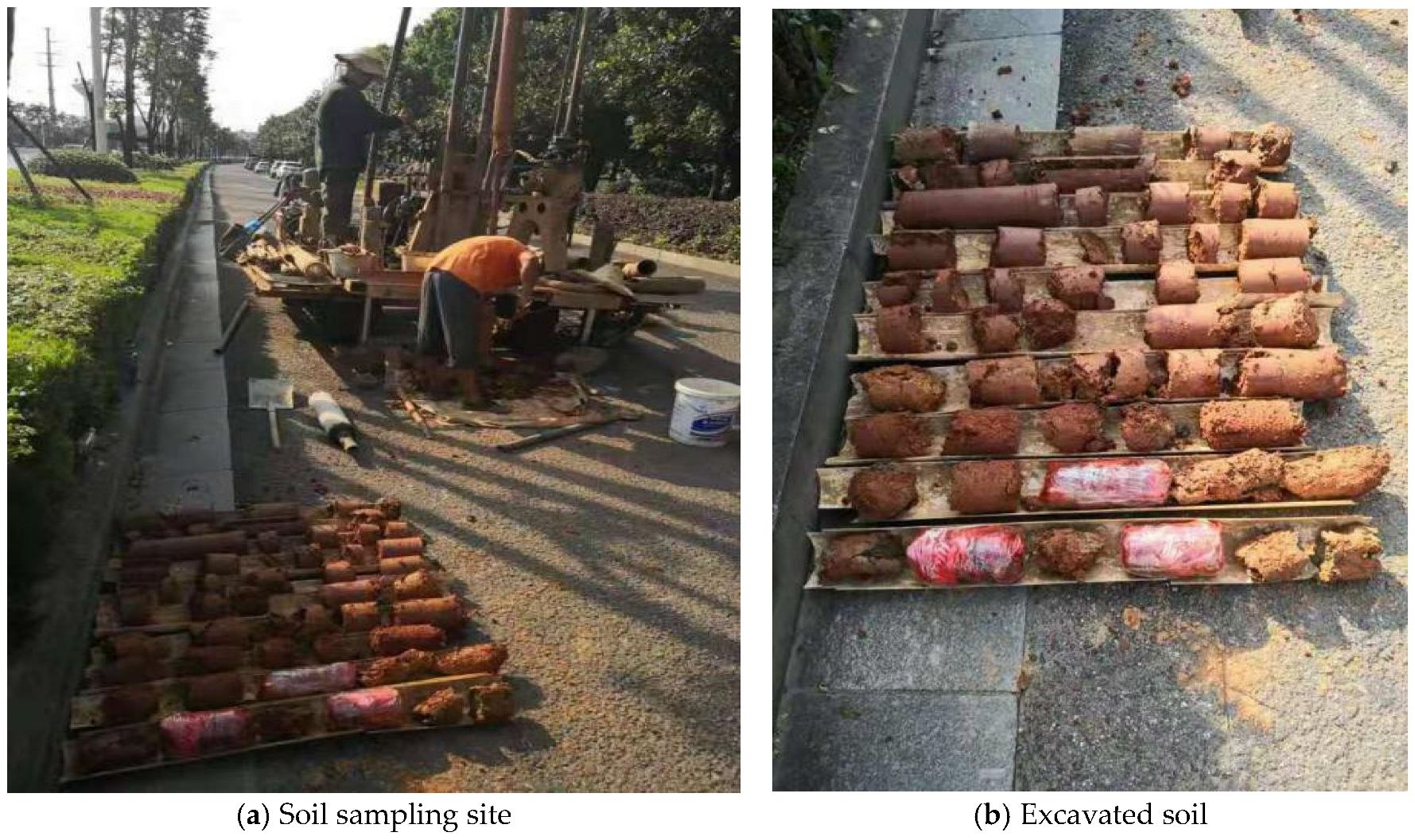
Soil samples were collected from Changsha City, China, representing typical residual hill and gully landforms with widely distributed powdery clay. The site exhibits medium-strength soil, commonly used as foundation-bearing layers in southern China. Two batches of in situ clayey soils were extracted, and disturbed samples were obtained from the same geological layer for comparative analysis. The soil samples are shown in Figure 1 and Figure 2. Two batches of in situ clayey soils were tested for various physical property indexes, mainly including particle composition, natural water content, plasticity index, and other common indexes, and the results are shown in

Table 1. Physical properties of the in situ soil samples under working condition I.

Working Condition	Particle Composition (%)			Natural Water Content w (%)	Natural Density ρ (g/cm3)	Proportion ds	Pore Ratio e	Plasticity Index Ip	Fluidity Index IL
	2~0.05 (mm)	0.05~0.005 (mm)	<0.005 (mm)
I-1	19	61	20	30.9	1.85	2.72	0.932	13.8	0.43
I-2	17	60	23	30.9	1.86	2.74	0.881	14.2	0.43
I-3	17	62	21	31.3	1.83	2.72	0.922	12.9	0.41
I-4	19	61	20	31.2	1.86	2.73	0.869	13.4	0.38
I-5	20	62	18	30.6	1.84	2.72	0.853	14.5	0.43
I-6	21	60	19	31.2	1.83	2.73	0.944	15.4	0.41
I-7	19	61	20	31.0	1.86	2.74	0.957	16.5	0.42
I-8	17	61	22	30.6	1.86	2.72	0.960	14.1	0.36
I-9	17	61	22	30.8	1.85	2.72	0.878	15.4	0.35

and

Table 2. Physical properties of the in situ soil samples under working condition II.

Working Condition	Particle Composition (%)			Natural Water Content w (%)	Natural Density ρ (g/cm3)	Proportion ds	Porosity (Math.) Ratio e	Plasticity Index Ip	Fluidity Index IL
	2~0.05 (mm)	0.05~0.005 (mm)	<0.005 (mm)
II-1	30	54	16	24.7	1.91	2.73	0.782	15.3	0.22
II-2	30	54	16	24.5	1.93	2.73	0.853	13.6	0.31
II-3	30	54	16	24.7	1.92	2.73	0.814	14.2	0.37

. The disturbed soil’s various physical indicators are shown in

Table 3. Physical properties of the disturbed soil samples under working condition I.

Working Condition	Particle Composition (%)			Natural Moisture Content w (%)	Natural Density ρ (g/cm3)	Specific Gravity ds	Porosity e	Plasticity Index Ip	Liquid Limit IL
	2~0.05 (mm)	0.05~0.005 (mm)	<0.005 (mm)
I-1	21	59	20	30.5	1.82	2.72	0.885	11.72	0.66
I-2	20	60	20	30.4	18.3	2.73	0.846	13.29	0.45
I-3	21	59	20	30.6	18.3	2.73	0.863	12.83	0.63
I-4	20	61	19	30.8	18.3	2.72	0.849	12.91	0.57
I-5	20	59	21	30.5	18.2	2.72	0.842	13.17	0.42
I-6	19	61	20	30.9	18.2	2.72	0.825	11.82	0.68
I-7	21	59	20	30.8	18.3	2.74	0.877	12.84	0.57
I-8	21	58	21	30.5	18.3	2.74	0.849	11.79	0.43
I-9	21	59	20	30.8	18.2	2.72	0.857	12.37	0.58

and

Table 4. Physical properties of the disturbed soil samples under working condition II.

Working Condition	Particle Composition (%)			Natural Moisture Content w (%)	Natural Density ρ (g/cm3)	Specific Gravity ds	Porosity e	Plasticity Index Ip	Fluidity Index IL
	2~0.05 (mm)	0.05~0.005 (mm)	<0.005 (mm)
II-1	32	54	18	24.5	1.87	2.72	0.756	16.7	0.31
II-2	32	54	18	25.0	1.87	2.72	0.834	15.4	0.34
II-3	32	54	18	25.1	1.86	2.71	0.732	15.9	0.45

.

Physical property characterization included particle composition analysis (2–0.05 mm, 0.05–0.005 mm, and <0.005 mm fractions), natural water content determination, density measurements, and specific gravity, porosity, plasticity, and fluidity indexes. As summarized in Table 1, Table 2, Table 3 and Table 4, the in situ soils (working condition I) showed natural water contents ranging from 30.6–31.3%, natural densities of 1.83–1.86 g/cm³, and plasticity indexes of 12.9–16.5. The disturbed soils exhibited similar particle size distributions but modified physical properties due to structure disturbance.

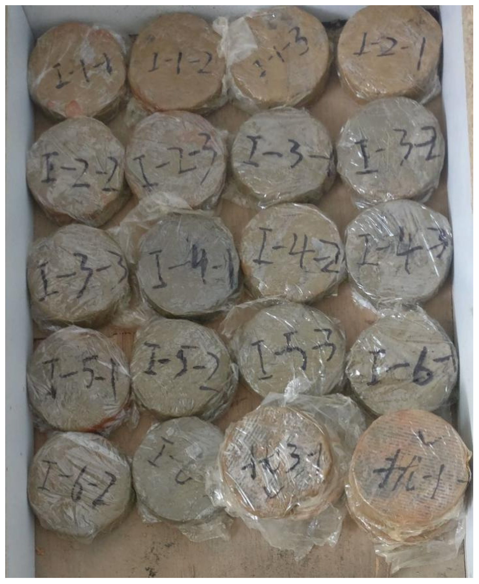
The in situ and disturbed soil specimens used in this test were both in an unsaturated state. The natural moisture content of in situ soil ranges from 24.7% to 31.3%, corresponding to a saturation level of approximately 85% to 92%. The disturbed soil was prepared after re-compaction by controlling the natural moisture content and density to match those of in situ soil; it did not undergo artificial saturation treatment and was also maintained in an unsaturated state. After sample preparation, the samples were sealed with plastic wrap and tested within 24 h to preserve their initial moisture content as much as possible. Specimen preparation followed Ref. [29] guidelines, accounting for the moisture content and density characteristics of powdery clay. All specimens were cylindrical with a 70 mm diameter and 20 mm height, prepared through two-layer compacted molding to ensure uniform density and consistency. Figure 3 illustrates representative prepared specimens.

2.3. Cyclic Single-Shear Test Setup

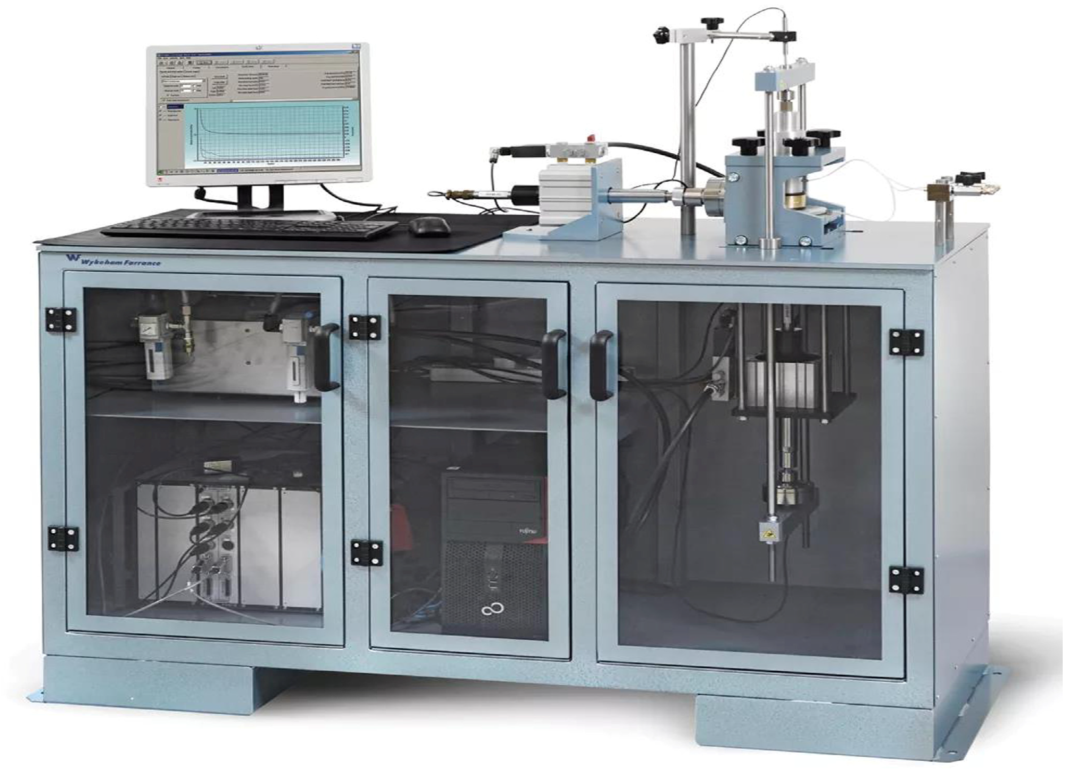
Cyclic single-shear tests were conducted using the British WFI WF25735 cyclic single-shear test system (Wykeham Farrance, Tring, UK) (Figure 4). This comprehensive apparatus comprises a double-action servo control brake, sophisticated control and digital data acquisition system, compressor, and specimen preparation equipment. The system is equipped with multiple sensors: vertical sensors (±5.0 kN), pressure sensors (1000 kPa), horizontal sensors (±5.0 kN), and displacement sensors (±25 mm), ensuring precise measurement throughout testing.

The cyclic single-shear system enables bi-directional pneumatic loading, with capabilities for various wave forms, including sinusoidal waves, random seismic inputs, and user-defined wave patterns. Test frequencies can reach up to 70 Hz. Laminated thin copper rings were employed to replicate in situ soil boundary conditions, facilitating constant volume and constant vertical pressure shear under both strain–controlled and stress–controlled conditions. The displacement transducer achieves 1 μm accuracy, while force transducers provide 0.001 kN precision. For each test cycle, 50 measurement points were collected to ensure comprehensive hysteresis curve characterization.

2.4. Loading Protocols and Data Acquisition

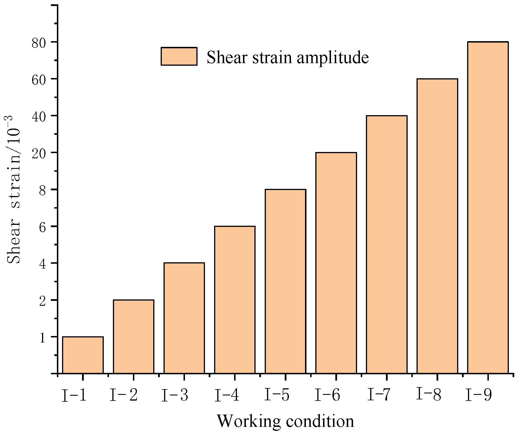
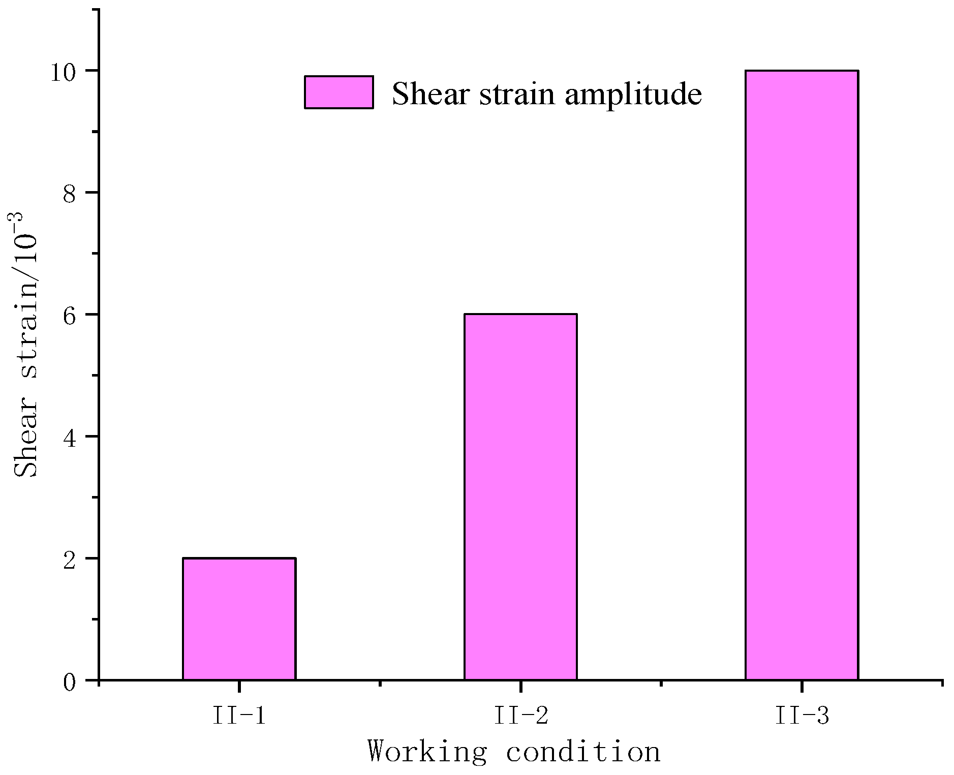
Two distinct loading protocols were implemented to investigate soil dynamic behavior. 1. Single-stage graded loading (Figure 5): This conventional approach employed multiple specimens, each subjected to a single shear strain amplitude to obtain stress–strain curves at specific strain levels. Ten loading cycles were applied per specimen, generating hysteresis curves across the complete strain range. This method minimizes cumulative deformation effects between different strain amplitudes. 2. Multi-stage cyclic loading (Figure 6): To simulate cumulative volume effects under earthquake loading, multiple cyclic loadings were applied to single specimens. Three shear strain amplitudes were selected, representing small (2 × 10⁻³), medium (6 × 10⁻³), and large (1 × 10⁻²) strains. Each specimen underwent 600 loading cycles at constant amplitude, enabling investigation of strain history effects on dynamic properties.

This loading method was adopted because cohesive soils exhibit high viscosity and irrecoverable deformation under cyclic loading, which can significantly influence the test results. Therefore, to study the variation in dynamic characteristic parameters of soil, a single graded loading mechanism was employed. This approach uses a single loading mechanism for multiple cyclic loadings to approximately simulate the cumulative volume effect on soil under earthquake loading. The soil experiences multiple shear deformations, and this method aims to understand the impact of these cumulative influences on the soil’s dynamic shear modulus ratio, as well as the damping ratio. Refs. [30,31,32,33] show that, in many cases of cyclic loading conditions, the magnitude of the shear strain on the cumulative volume effect will have a greater impact. Therefore, the shear strain amplitude is set as small strain, medium strain, and large strain, respectively.

All tests maintained consistent conditions: 50 kPa consolidation pressure, equal-amplitude sinusoidal loading at a 1 Hz frequency, undrained conditions, and strain-controlled loading, with 50 data points recorded per cycle. For each working condition, three replicate specimens were tested to ensure result reliability.

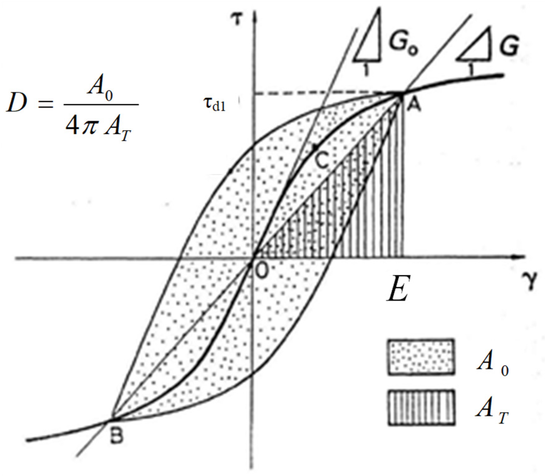
For the cyclic single shear test, hysteresis loops depicting the dynamic relationship between shear τ_d and shear strain stress γ_d at each instant are generated based on their determinations. These loops are illustrated in Figure 7. The definitions of the dynamic shear modulus G_d and damping ratio D can be expressed as Equations (1) and (2), respectively.

G_d = (|τ_d1| + |τ_d2|)/(|γ_d1| + |γ_d2|)

(1)

D = A₀/(4πA_T)

(2)

where τ_d1 and τ_d2 are the positive and negative highest dynamic shear stress, and γ_d1 and γ_d2 are the positive and negative maximum dynamic shear strain. The triangle AOE’s area is represented by A_T, where A_T can be calculated by $A_T={\displaystyle \frac{1}{2}}\cdot {\gamma }_{d1}\cdot {\tau }_{d1}$, and the hysteresis loop’s area, A₀, represents the energy used in one cycle of cyclic loading, where A₀ can be calculated by $A_0=\oint \tau d\gamma$.

3. The Cyclic Single-Shear Test Results

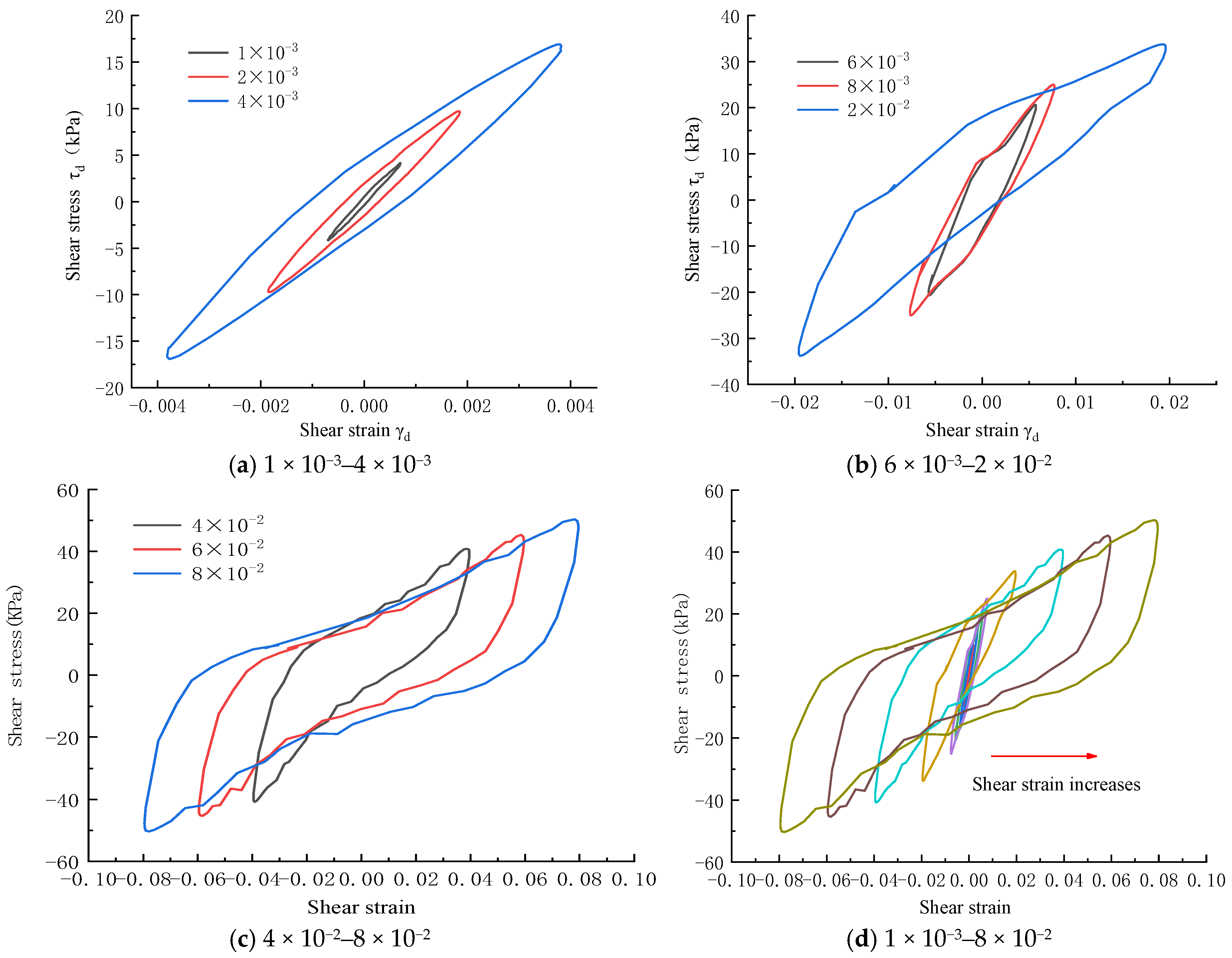
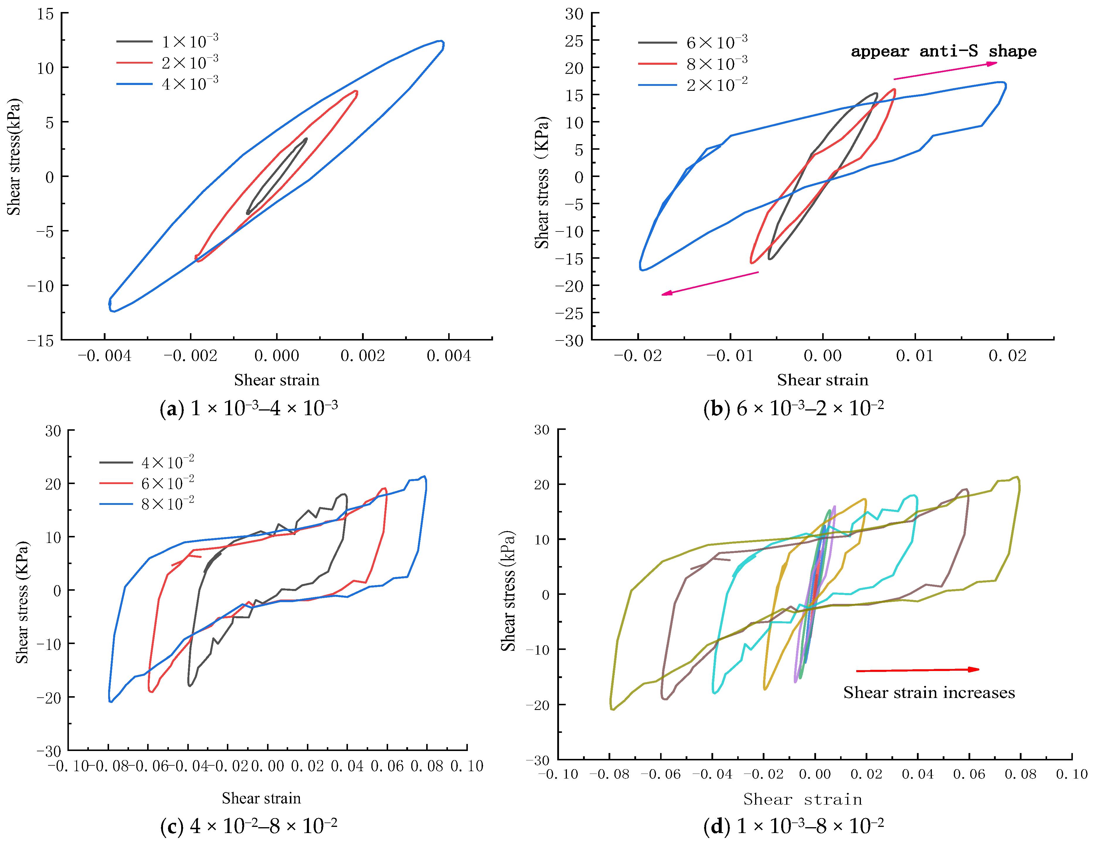
The hysteresis curves presented for each strain amplitude are based on the measured results of a single representative specimen selected from the set of three parallel specimens. Hysteresis curves for the in situ soils in the shear strains γ = 1 × 10⁻³–4 × 10⁻³, 6 × 10⁻³–2 × 10⁻², and 4 × 10⁻²–8 × 10⁻², and full shear strain ranges, are given in Figure 8. Prior to a shear strain of 8 × 10⁻³, the in situ soil hysteresis loop exhibits an elliptical shape, with the area of the ellipse gradually increasing as the shear strain amplitude rises. However, when the shear strain exceeds 2 × 10⁻², the hysteresis curve adopts an S-shape (i.e., the slope of the tangent line of the stress–strain hysteresis decreases suddenly, and increases slowly when approaching the stress change sign, and then increases dramatically before the strain turns to the other side). The “S-shaped” feature of the hysteresis curve is most significant at shear strain amplitudes up to 8 × 10⁻². From the above, the following conclusion can be obtained: with the increase in strain amplitude, the hysteresis circle gradually changes from an ellipse with a small inclination angle to a curve with a larger inclination angle, with an obvious “S-shape” (Figure 8d), and the encircled area increases, which indicates the soil’s enhanced capacity to dissipate energy. The stress–strain relationship exhibits a strong nonlinearity and hysteretic nature.

The hysteresis curves of the disturbed soil at the shear strain γ = 1 × 10⁻³–4 × 10⁻³, 6 × 10⁻³–2 × 10⁻², and 4 × 10⁻²–8 × 10⁻², and the hysteretic curve within the entire shear strain range are given in Figure 9. Compared with the in situ soil, the hysteresis curve of the disturbed soil starts to show an “S-shaped” shape at a shear strain of 8 × 10⁻³, which is smaller than the shear strain critical value of the in situ soil, and under all circumstances, the peak shear stress of the disturbed soil is lower than that of the in situ soil, which is manifested in the flattening its the hysteresis curve compared with that of the in situ soil (Figure 9d).

After determining the damping ratio and dynamic shear modulus, the parameter values for the in situ soil, as well as the disturbed soil at different amplitudes of shear strain, can be obtained, as shown in

Table 5. Single-shear test data for condition I in situ soil.

Specimen	Positive Maximum Shear Strain γd1	Negative Maximum Shear Strain γd2	Positive Maximum Shear Stress τd1 (kPa)	Negative Maximum Shear Stress τd2 (kPa)	Hysteresis Loop Area A0	Area of Triangle Abc AT	Dynamic Shear Modulus Gd (kPa)	Damping Ratio D
I-1	7.02 × 10−4	−7.02 × 10−4	4.152	−4.152	0.001	0.006	5912.177	5.580 × 10−2
I-2	1.86 × 10−3	−1.86 × 10−3	9.735	−9.735	0.009	0.036	5246.469	8.247 × 10−2
I-3	3.81 × 10−3	−3.81 × 10−3	16.924	−16.924	0.042	0.129	4437.752	1.044 × 10−1
I-4	5.73 × 10−3	−5.73 × 10−3	20.656	−20.656	0.100	0.237	3604.649	1.344 × 10−1
I-5	7.70 × 10−3	−7.70 × 10−3	24.989	−24.989	0.181	0.385	3243.633	1.499 × 10−1
I-6	1.96 × 10−2	−1.96 × 10−2	33.779	−33.779	0.670	1.323	1724.572	1.611 × 10−1
I-7	3.96 × 10−2	−3.96 × 10−2	40.742	−40.742	2.003	3.226	1029.176	1.976 × 10−1
I-8	5.96 × 10−2	−5.96 × 10−2	45.333	−45.333	3.701	5.401	761.081	2.182 × 10−1
I-9	7.95 × 10−2	−7.95 × 10−2	50.318	−50.318	5.701	8.003	632.728	2.267 × 10−1

and

Table 6. Cyclic single-shear test data under condition I in disturbed soil [34].

Specimen	Positive Maximum Shear Strain γd1	Negative Maximum Shear Strain γd2	Positive Maximum Shear Stress τd1 (kPa)	The Negative Maximum Shear Stress τd2 (kPa)	Hysteresis Loop Area A0	Area of Triangle abc AT	Dynamic Shear Modulus Gd (kPa)	Damping Ratio D
I-1	7.002 × 10−4	−7.002 × 10−4	3.484	−3.484	0.001	0.005	4974.918	7.833 × 10−2
I-2	1.880 × 10−3	−1.880 × 10−3	7.898	−7.898	0.009	0.030	4201.670	9.394 × 10−2
I-3	3.896 × 10−3	−3.896 × 10−3	12.260	−12.260	0.036	0.096	3146.945	1.205 × 10−1
I-4	5.829 × 10−3	−5.829 × 10−3	14.617	−14.617	0.073	0.170	2507.773	1.358 × 10−1
I-5	7.793 × 10−3	−7.793 × 10−3	15.563	−15.563	0.096	0.243	1997.049	1.261 × 10−1
I-6	1.979 × 10−2	−1.979 × 10−2	15.970	−15.970	0.413	0.632	807.155	2.078 × 10−1
I-7	3.971 × 10−2	−3.971 × 10−2	16.247	−16.247	1.111	1.290	409.137	2.741 × 10−1
I-8	5.958 × 10−2	−5.958 × 10−2	17.630	−17.630	2.325	2.101	295.889	3.523 × 10−1
I-9	7.955 × 10−2	−7.955 × 10−2	20.094	−20.094	3.903	3.197	252.592	3.886 × 10−1

.

4. Dynamic Constitutive Model of Cohesive Soils

The analysis in Section 2 has elucidated that cohesive soils, under cyclic loading, manifest nonlinear, hysteretic stress–strain relationships, along with deformation accumulation. The soil dynamic constitutive model, representing the stress–strain relationship under dynamic loading, serves as a fundamental framework for characterizing soil dynamics. It constitutes a central aspect of soil dynamics research and provides a crucial foundation for analyzing various issues related to soil dynamic instability.

Assuming that the amplitude of shear strain is identified, the soil’s shear modulus and damping ratio may generally be computed. The soil dynamic shear modulus usually indicates the soil stiffness, which is usually related to the amplification coefficient in dynamic analyses, such as earthquakes, and the damping ratio typically expresses the energy dissipation capacity of soil, which is strongly associated with the stress and strain response of the superstructure.

In contrast to static difficulties, soils under dynamic stresses, such as earthquakes, typically exhibit dynamic characteristics (dynamic shear modulus and damping ratio) that are not constant, but are related to the loading process and loading history. In this section of the study, the experimental data in Section 2 will be used as a basis to clarify the guidelines for variation in the dynamic parameters of soils under dynamic loading.

4.1. Soil Dynamic Model

B.O.Harding [35] was the first to introduce G_max to describe the connection between the average modulus of dynamic shear G, the damping proportion λ, and the magnitude of the dynamic shear strain γ_s:

$$G={\displaystyle \frac{G_{max}}{1+\frac{{\gamma }_s}{{\gamma }_r}}}$$

(3)

$$\lambda ={\displaystyle \frac{4}{\pi }}{\displaystyle \frac{1}{1-\frac{G}{G_{max}}}}\left[1-{\displaystyle \frac{\frac{G}{G_{max}}}{1-\frac{G}{G_{max}}}}ln{\displaystyle \frac{G_{max}}{G}}\right]-{\displaystyle \frac{2}{\pi }}$$

(4)

In the above equation, γ_r denotes the reference strain. It is usually obtained by fitting the test data. In the small strain range, the model and the test value can still be a good match, but when the strain exceeds a certain value, the damping ratio is significantly larger than the actual value and grows rapidly. At the same time, the hyperbolic model description is simpler, and there is only one coefficient, namely, the reference shear strain that can be varied, but the acquisition of this coefficient also requires the existence of strong theoretical knowledge, which is not easy to accurately obtain, so the fitting effect is not ideal.

Another model is the Ramberg–Osgood model [36], whose expression is shown below:

$${\displaystyle \frac{G}{G_{\max }}}={\displaystyle \frac{1}{1+\alpha {\left|\frac{\tau }{C_1{\tau }_{\max }}\right|}^{R-1}}}$$

(5)

In the above, τ_max is the maximum shear stress. C₁, R, and α are fitting parameters. The damping ratio in this model is determined by the following equation:

$$\lambda ={\displaystyle \frac{2}{\pi }}{\displaystyle \frac{R-1}{R+1}}\left(1-{\displaystyle \frac{G}{G_{\max }}}\right)$$

(6)

A more commonly used expression for the soil–body principal relationship is the Daredelli model:

$${\displaystyle \frac{G_d}{G_{d\max }}}={\displaystyle \frac{1}{1+{\left({\gamma }_{\alpha }/{\gamma }_{ref}\right)}^{\alpha }}}$$

(7)

α represents the attenuation parameter defining the modulus curve’s behavior; γ_a stands for the shear strain amplitude; γ_ref denotes the reference shear strain amplitude; G_dmax signifies the maximum shear strain experienced; G_d represents the dynamic shear modulus, corresponding to γ_a; and the expression for the damping ratio is

$$D={\displaystyle \frac{D_{\max }\cdot {\left({\gamma }_a/{\gamma }_{ref}\right)}^{\beta }}{1+{\left({\gamma }_a/{\gamma }_{ref}\right)}^{\beta }}}$$

(8)

The Ramberg-Osgood model expresses G_max in terms of shear stress ratio, and it is more convenient to study the problem using the shear strain ratio with lower error. The Darredenli model can be used to analyze the dynamic properties of cohesive soils, but there are only two morphology parameters in the formula, which are more binding for the shear stress–strain relationship curve. Therefore, it is natural to think about whether there is an expression of the relationship containing multiple parameters, each parameter only affects one aspect of the morphology of the principal relationship curve, which can accurately describe the stress–strain relationship in the full strain range under the coupling effect of multiple parameters.

This paper, focusing on analyzing actual data and contrasting different theoretical models, proposes to use the Davidenkov model, containing three parameters, to describe the relationship from dynamic strain to dynamic shear modulus, as well as the correlation between dynamic shear strain and the damping ratio:

$${\displaystyle \frac{G}{G_{\max }}}=1-{\left[{\displaystyle \frac{{\left(\frac{{\gamma }_s}{{\gamma }_0}\right)}^{2B}}{1+{\left(\frac{{\gamma }_s}{{\gamma }_0}\right)}^{2B}}}\right]}^A$$

(9)

$$\lambda ={\lambda }_{\max }{\left(1-{\displaystyle \frac{G}{G_{\max }}}\right)}^{\beta }$$

(10)

in which A, B, and γ₀ are connected to the soil mechanical features through fitting parameters.

The damping ratio serves as a quantitative measure of the energy dissipation properties exhibited by geotechnical materials subjected to cyclic loading. When the stress–strain relationship skeleton curve follows the Davidenkov model, and the hysteresis curve is constructed based on Masing’s law, the formula for the damping ratio of the soil can be derived as:

$$D={\displaystyle \frac{2}{\pi }}\cdot \left\{{\displaystyle \frac{{\gamma }_c^2-2\cdot {\int }_0^{{\gamma }_c}\gamma \cdot H\left(\gamma \right)d\gamma }{{\gamma }_c^2\cdot \left[1-H\left({\gamma }_c\right)\right]}}-1\right\}$$

(11)

In the above, γ_c is the shear strain value corresponding to the change in shear modulus.

From Equations (9) and (10), the formula for the damping ratio is not independent, and it is related to the expression of the maximum dynamic shear modulus. Additionally, the damping ratio and maximal dynamic shear modulus may be represented as:

$${\displaystyle \frac{G}{G_{\max }}}=1-{\left[{\displaystyle \frac{{\left(\frac{{\gamma }_s}{{\gamma }_0}\right)}^{2B}}{1+{\left(\frac{{\gamma }_s}{{\gamma }_0}\right)}^{2B}}}\right]}^A$$

(12)

$$\lambda ={\lambda }_{\max }{\left[{\displaystyle \frac{{\left(\frac{{\gamma }_s}{{\gamma }_0}\right)}^{2B}}{1+{\left(\frac{{\gamma }_s}{{\gamma }_0}\right)}^{2B}}}\right]}^{A\beta }$$

(13)

4.2. Parameter Sensitivity Analysis

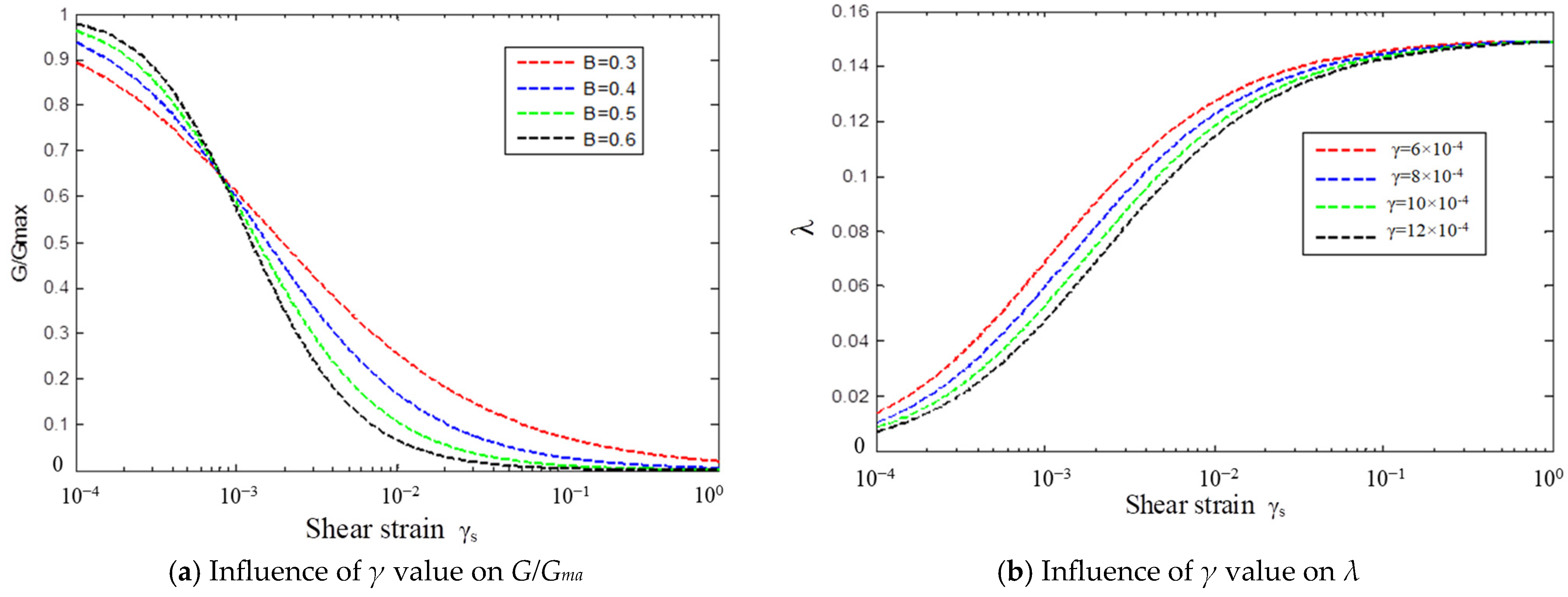
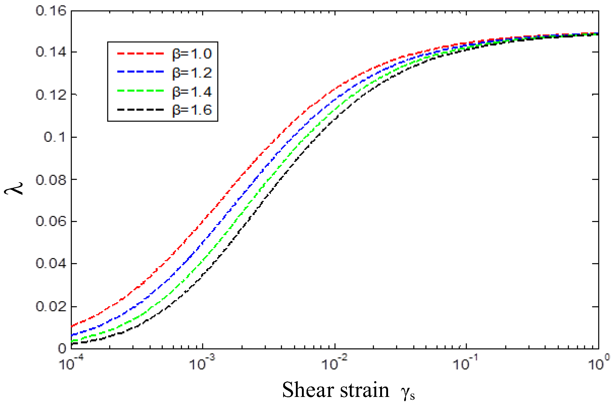
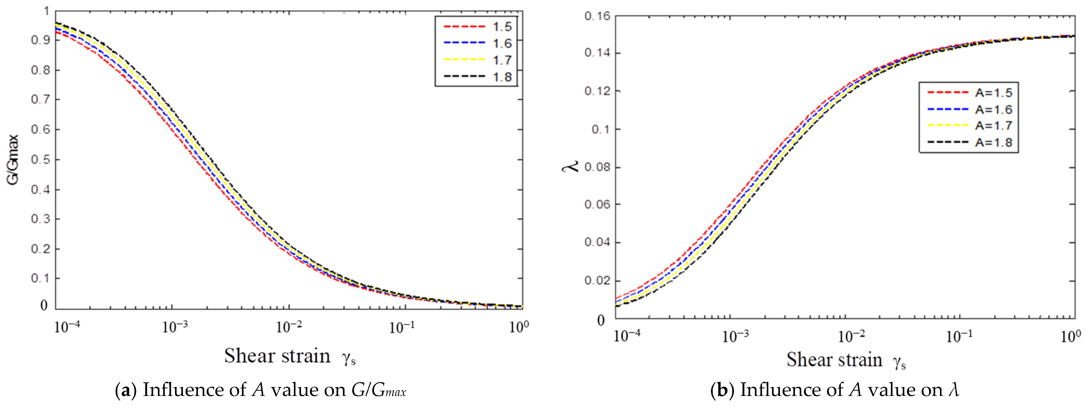
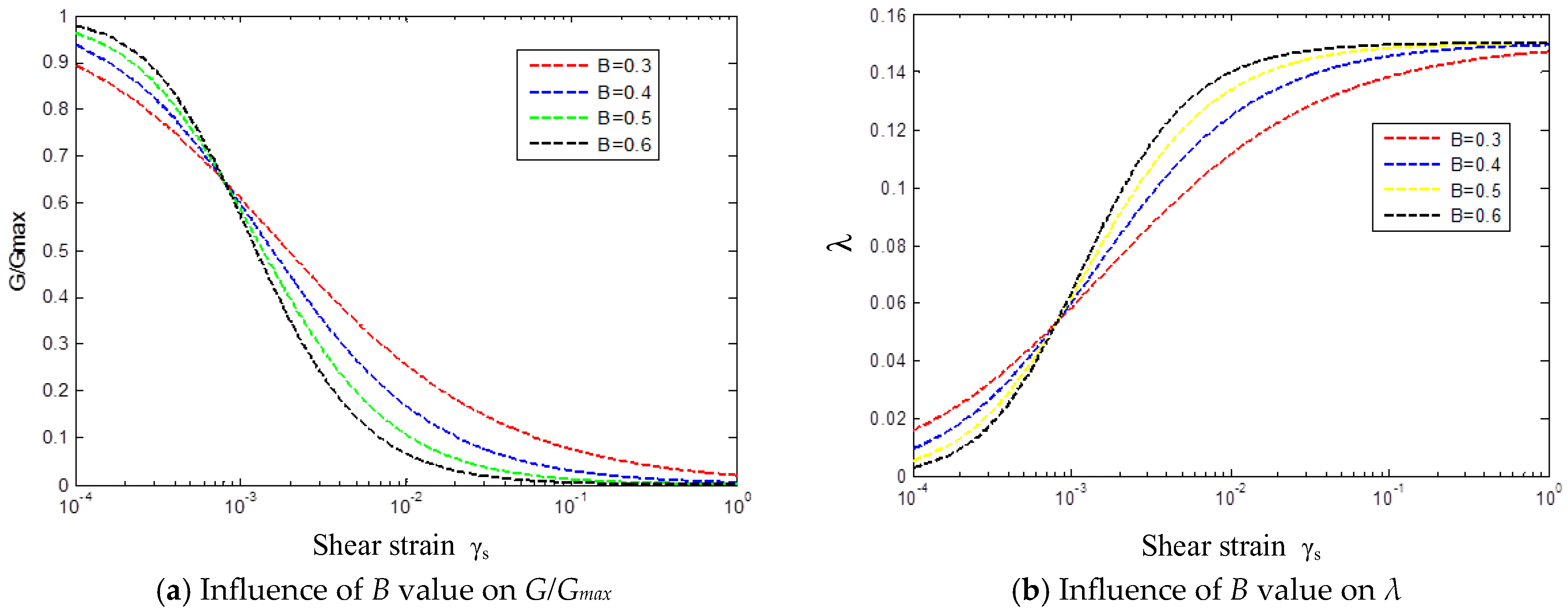
Through Equations (12) and (13), it can be seen that the Davidenkov model contains three fitting parameters, A, B, and γ₀. Before quantitatively analyzing the experimental data, to be able to illustrate the outcomes of the various parameter values on the curve of the law, a sensitivity analysis of the parameters is performed first: from the three parameters, make one parameter take a different value, and make the other two parameters a certain value, consider the influence of the parameter changes on the law of change curve, and then clarify the influence of each parameter on the structure of the curve law. The impact of parameter A on the damping ratio λ and G/G_max, which means the maximum dynamic shear modulus ratio, is depicted in Figure 10. Parameter B’s effect on the damping ratio λ and G/G_max is seen in Figure 11. Figure 12 shows the influence of parameter γ on the G/G_max and λ, and Figure 13 demonstrates the impact of β value on λ.

The following conclusions can be drawn from Figure 10, Figure 11, Figure 12 and Figure 13:

(1)

As can be seen in Figure 10, with a decrease in the A value, the G/G_max curve shows an overall downward trend. For the same shear strain, taking different values of A, the value of G/G_max is not much different; with a decrease in the A value, the damping ratio change curve shows an upward shift trend. At the same time, for the same shear strain amplitude, if the A value is different, the magnitude of the change in the damping ratio is not large. The change in the A value has less influence on the curve fitting effect, and mainly affects the up and down “telescoping” change in the curve.

(2)

As can be seen from Figure 11, with the change in the B value, the G/G_max curve shape shows the characteristics of the “S-shape”. At small strain amplitudes, with the increase in the B value, the curve gradually shows a “convex” form. If the shear strain amplitude exceeds a specific value, the G/G_max value decreases gradually as the B value increases, reacting to the curve slope, the curve slope gradually increases, and the curve becomes “downward convex”. After the shear strain amplitude exceeds a specific value, with the increase in the B value, the reduction speed of the G/G_max value increases gradually, which is reflected in the slope of the curve: the slope of the curve increases gradually, and the curve shows “lower convexity”. It can be seen from the above analysis that the B value mainly affects the degree of “concavity” of the G/G_max and λ curves.

(3)

The influence of the law for the γ₀ value on the curve is similar to that of the A value, and from the curve change graph, it is evident that the influence of the γ₀ value on the curve is greater than that of the A value.

(4)

The influence of the β value on the damping ratio curve is mainly manifested in the up and down shift of the influence curve, and the curve trend is consistent: as the shear strain is small, rapid increases in the damping ratio are seen. Therefore, the damping ratio increases at a slower pace when the shear strain is high.

The aforementioned curves offer a visual representation of the multi-parameter soil shear modulus and damping ratio, illustrating their susceptibility to changes in various parameters. The soil dynamic shear modulus, as well as the damping ratio, are influenced not only by the shear strain amplitude and loading rate, but also by the soils’ mechanical properties, such as water content, gradation, and grain size, among others. Therefore, for a specific soil specimen, the soil shear modulus and damping ratio curves are distinct, which is reflected in the mechanical model; the values of γ₀ and the β parameters will be different. There are differences in the shape of the curves, tensile, and convexity. However, these differences do not affect the general trend of the mechanical parameters.

4.3. Comparison of Soil Dynamic Constitutive Modeling and Test Results

Soil dynamic testing serves as a fundamental method for investigating soil dynamic characteristics. It enables the discernment of distinct mechanical properties among various soil types and states, but its efficacy is contingent upon conducting tests on specific soil samples under defined conditions. Ref. [37] indicates that soil shear strain under seismic activity typically falls within the range of 2 × 10⁻⁴–2.0 × 10⁻³; the soil–structure contact can extend to even greater extents. The strain amplitudes attained indoors during dynamic soil property testing typically surpass those experienced outdoors. Cyclic single shear tests serve as an effective means to replicate soil units subjected to ideal dynamic loads, such as seismic stresses, within laboratory settings.

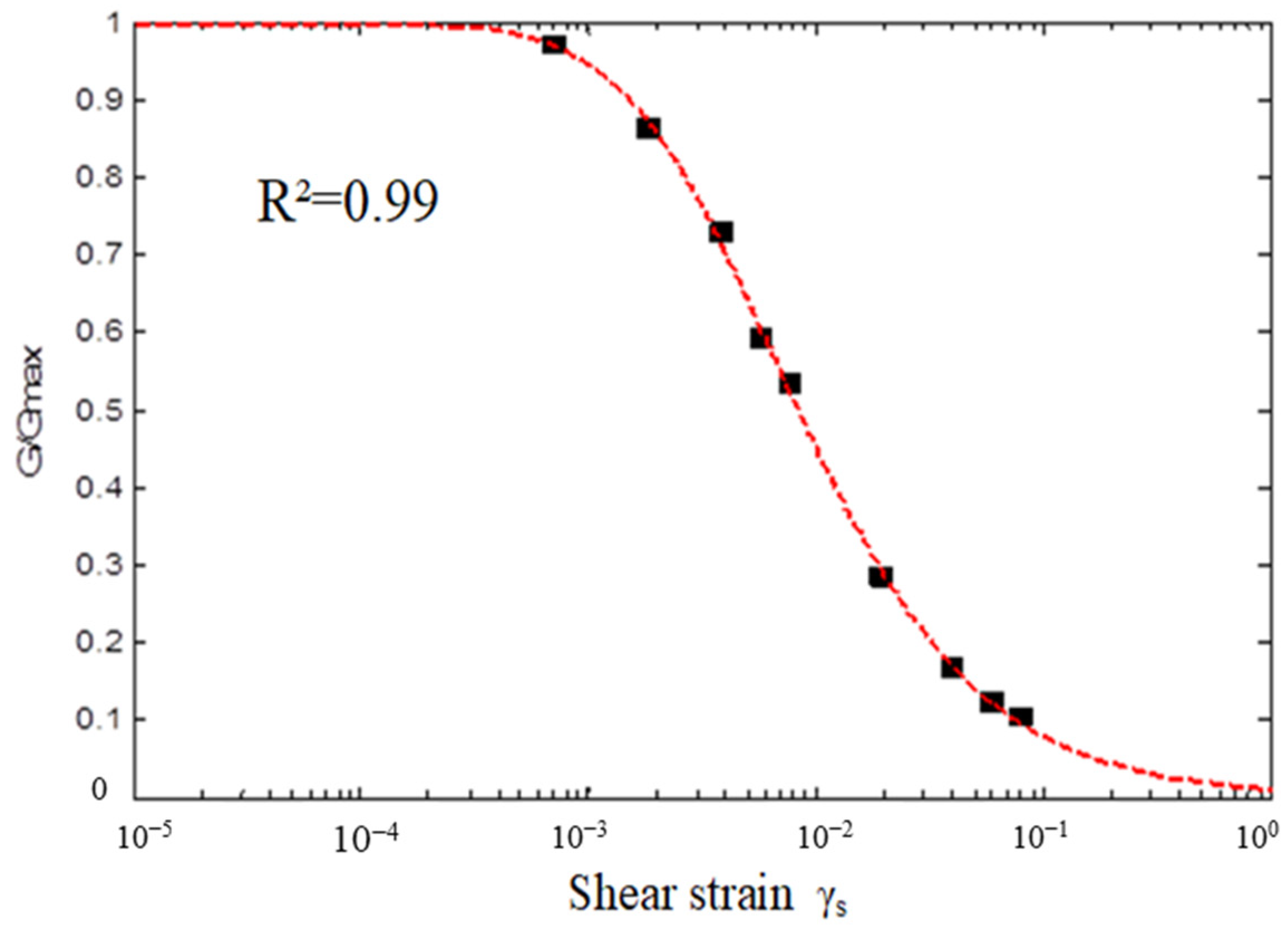
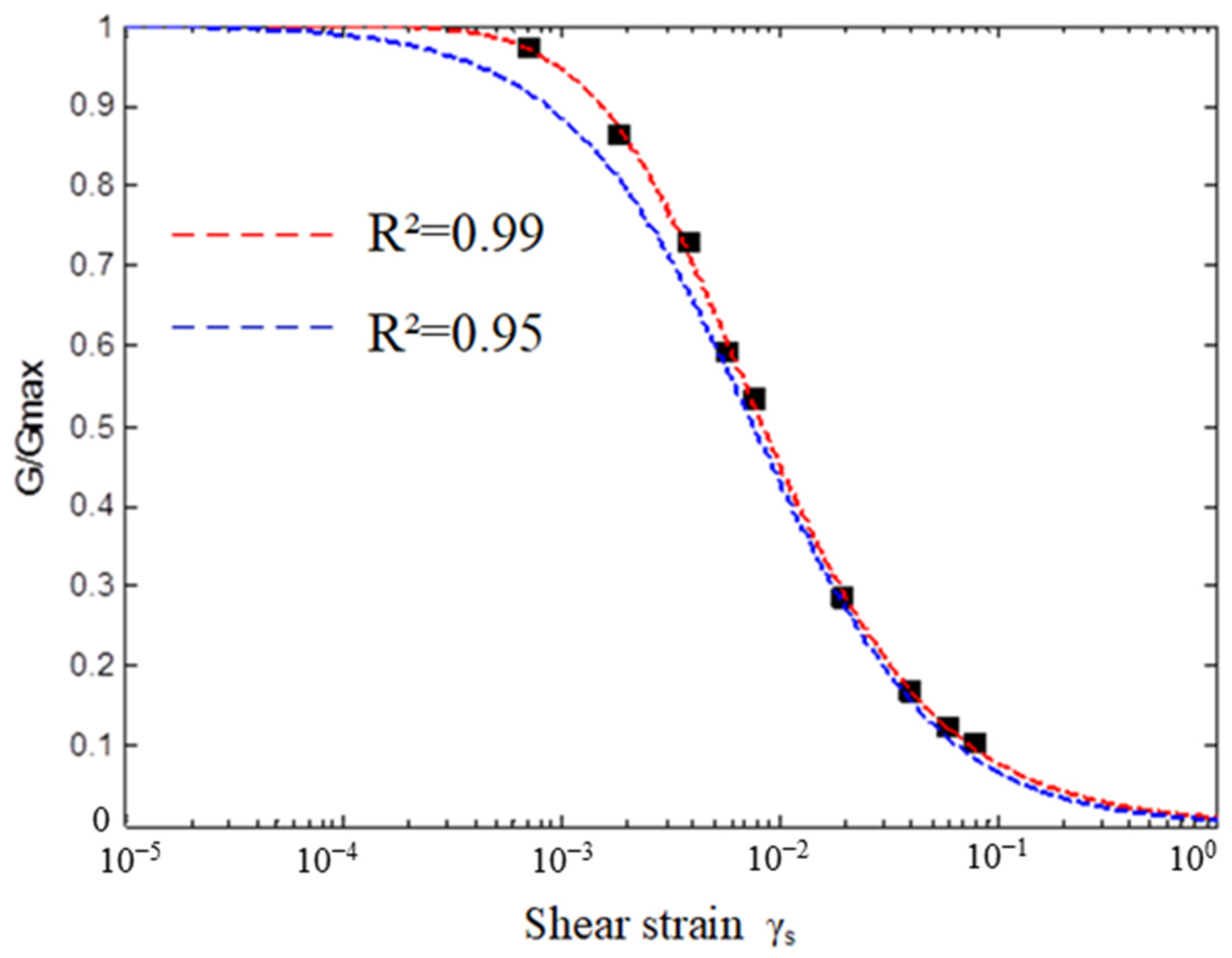
Figure 14 shows the contrast between the curves obtained from the dynamic shear modulus test data based on the three-parameter model, fitted with the test data. The least squares method was used for nonlinear regression fitting of the parameters, where the fitted parameters are B = 0.45, A = 2.62, and γ₀ = 22.4 × 10⁻⁴. The expression of the Davidenkov model function is:

$${\displaystyle \frac{G}{G_{\max }}}=1-{\left[{\displaystyle \frac{{\left(\frac{{\gamma }_s}{22.4\times {10}^{-4}}\right)}^{0.9}}{1+{\left(\frac{{\gamma }_s}{22.4\times {10}^{-4}}\right)}^{0.9}}}\right]}^{2.62}$$

(14)

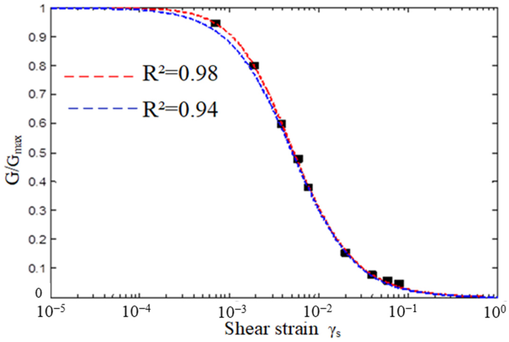
As can be seen from the figure, the three-parameter Davidenkov model can well represent the change rule for G/G_max with shear strain. The values of (γ_s − G/G_max), obtained from the test in the full domain of shear strain, fall completely on the curve, and the fitted curve has a high degree of match with the test data. Figure 15 shows the Davidenkov and Daredalli model with the test data comparison curve. It can be seen that when the shear strain amplitude is small, the G/G_max value obtained by fitting is smaller than the test measured. Considering the aforementioned analysis, apparently, the three-parameter Davidenkov model can better represent the γs − G/G_max variation pattern.

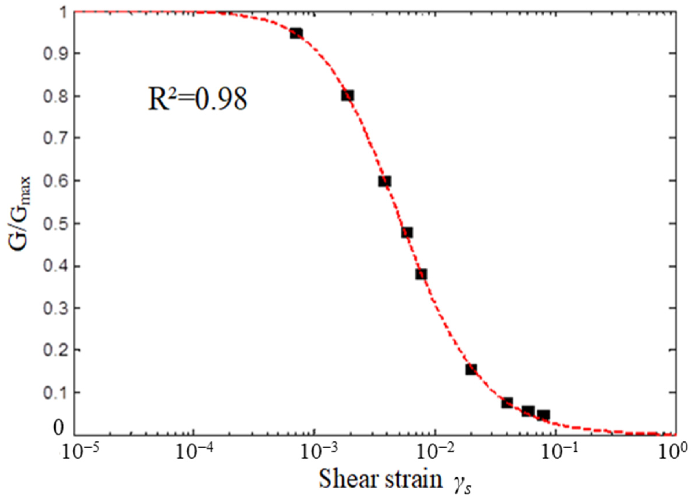
Figure 16 contrasts the experimental data with the theoretical data on the disturbed soil. The disturbed soil curve morphology parameters are B = 0.58, A = 1.43, and γ₀ = 35.4 × 10⁻⁴. For the disturbed soil, the Davidenkov model function expression is:

$$G=1-{\left[{\displaystyle \frac{{\left(\frac{{\gamma }_s}{35.4\times {10}^{-4}}\right)}^{1.16}}{1+{\left(\frac{{\gamma }_s}{35.4\times {10}^{-4}}\right)}^{1.16}}}\right]}^{1.43}$$

(15)

As can be seen from Figure 16, the three-parameter Davidenkov model can well represent the change rule for G/G_max with shear strain. The scatter points of (γ_s − G/G_max), obtained from the test, fall completely on the curve, and it is evident that the fitted curves have a high match with the experimental data. For the single-parameter Daredalli model fitting curve, as the shear strain is tiny, the fitted G/G_max value corresponding to the shear strain amplitude is less than the test observed value (Figure 17). Considering the aforementioned analysis, it can be seen that the three-parameter Davidenkov model is able to more accurately depict the γ_s − G/G_max variation pattern.

In comparison to the in situ soil, there is not much of a difference between the one-parameter and three-parameter models for the disturbed soil. This is mainly due to the fact that the disturbed soil is the soil whose natural structure has been damaged or water content has been changed, and its sensitivity to the three parameters is low.

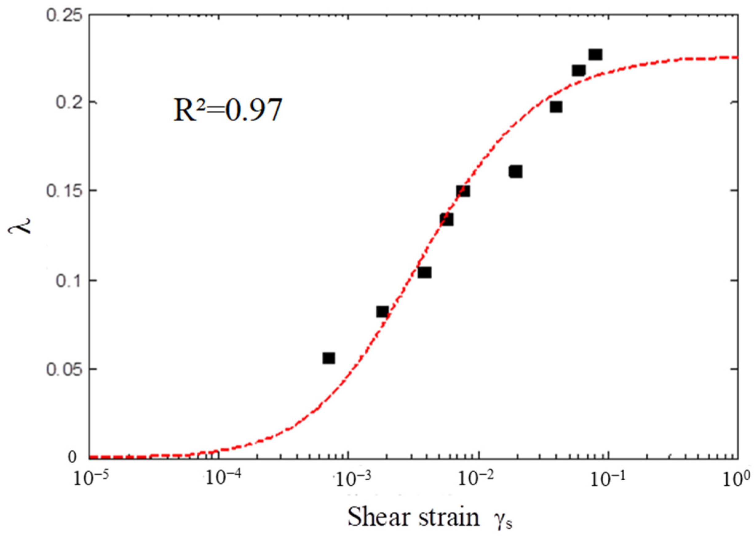
The Davidenkov damping ratio fitted curve is shown in Figure 18, in comparison with the experimental data. The three parameters are B = 0.45, A = 2.62, and γ₀ = 22.4 × 10⁻⁴, the maximum value of the sample damping ratio is 0.227, and the independent variable of the fitted curve form is β = 0.54. The functional relationship between λ and the amplitude of the shear strain, γ_s, after the fit is shown below:

$$\lambda =0.227{\left[{\displaystyle \frac{{\left(\frac{{\gamma }_s}{22.4\times {10}^{-4}}\right)}^{0.9}}{1+{\left(\frac{{\gamma }_s}{22.4\times {10}^{-4}}\right)}^{0.9}}}\right]}^{1.41}$$

(16)

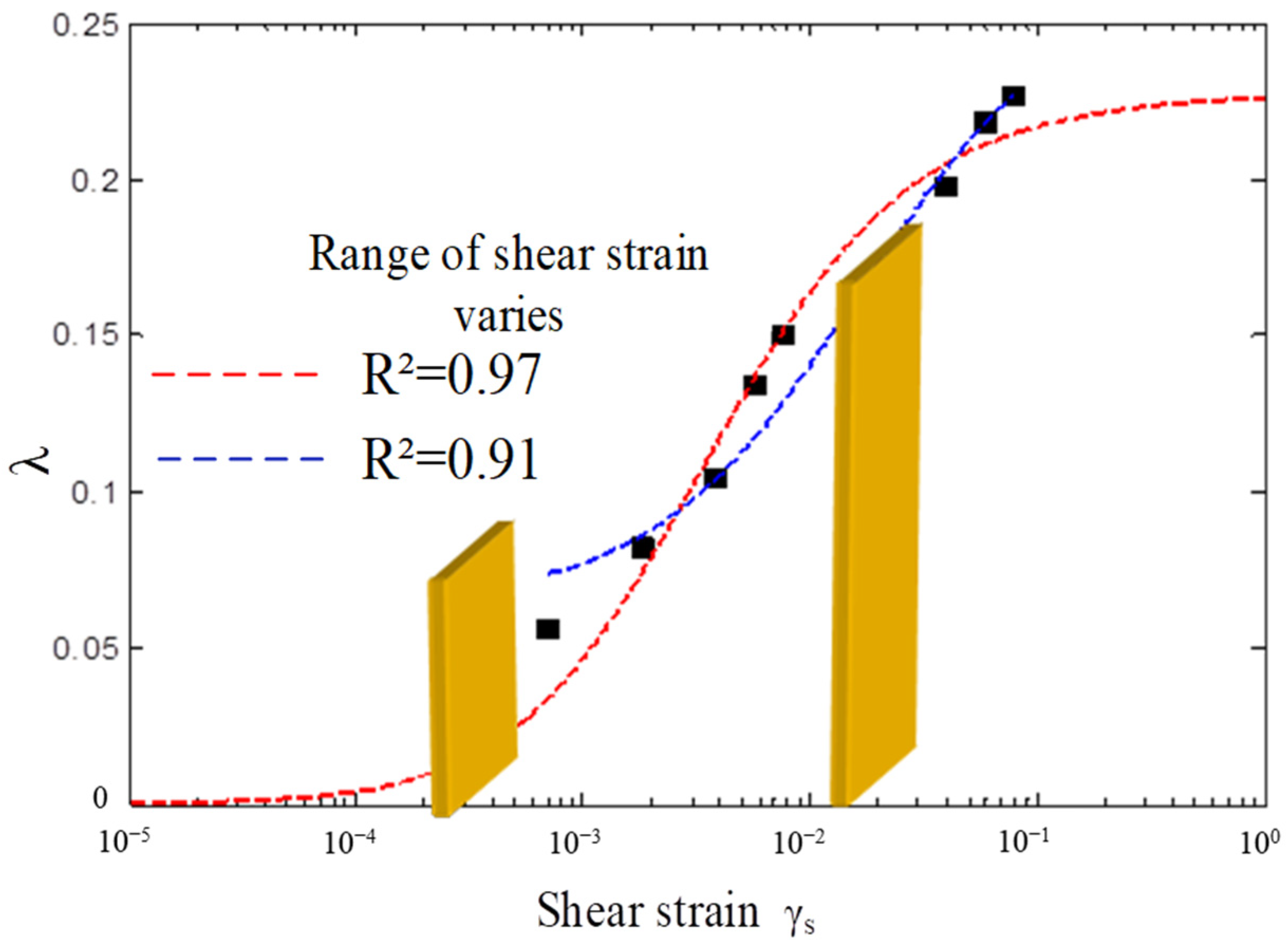
Comparison of different models of the in situ soil damping ratio under seismic action is shown in Figure 19. Typically, the shear deformation of the soil under seismic action ranges from 2 × 10⁻⁴ to 2 × 10⁻², and within this range of shear strain amplitude (between the yellow areas), the three-parameter Davidenkov model is used for a more precise description of shear strain–damping ratio.

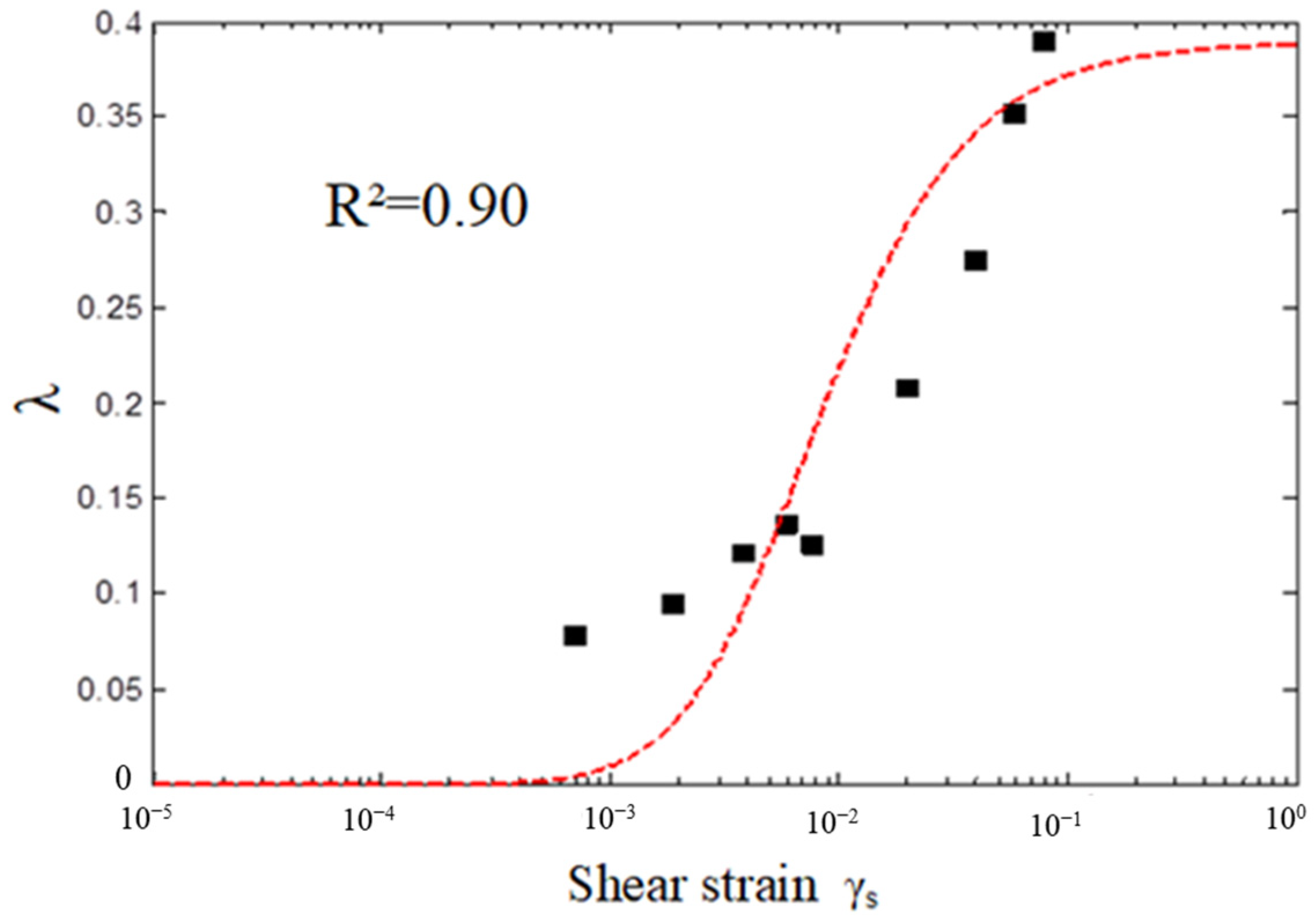
Figure 20 shows the comparison of the theoretical curve of the disturbed soil with the test data, and the parameter values are B = 0.58, A = 1.43, γ₀ = 35.4 × 10⁻⁴, the maximum value of the sample damping ratio is 0.389, and the independent variable of the fitted curve form is β = 1.86. The functional relationship between λ and the shear strain amplitude γ_s, after fitting, is shown as follows:

$$\lambda =0.389{\left[{\displaystyle \frac{{\left(\frac{{\gamma }_s}{35.4\times {10}^{-4}}\right)}^{1.16}}{1+{\left(\frac{{\gamma }_s}{35.4\times {10}^{-4}}\right)}^{1.16}}}\right]}^{2.3}$$

(17)

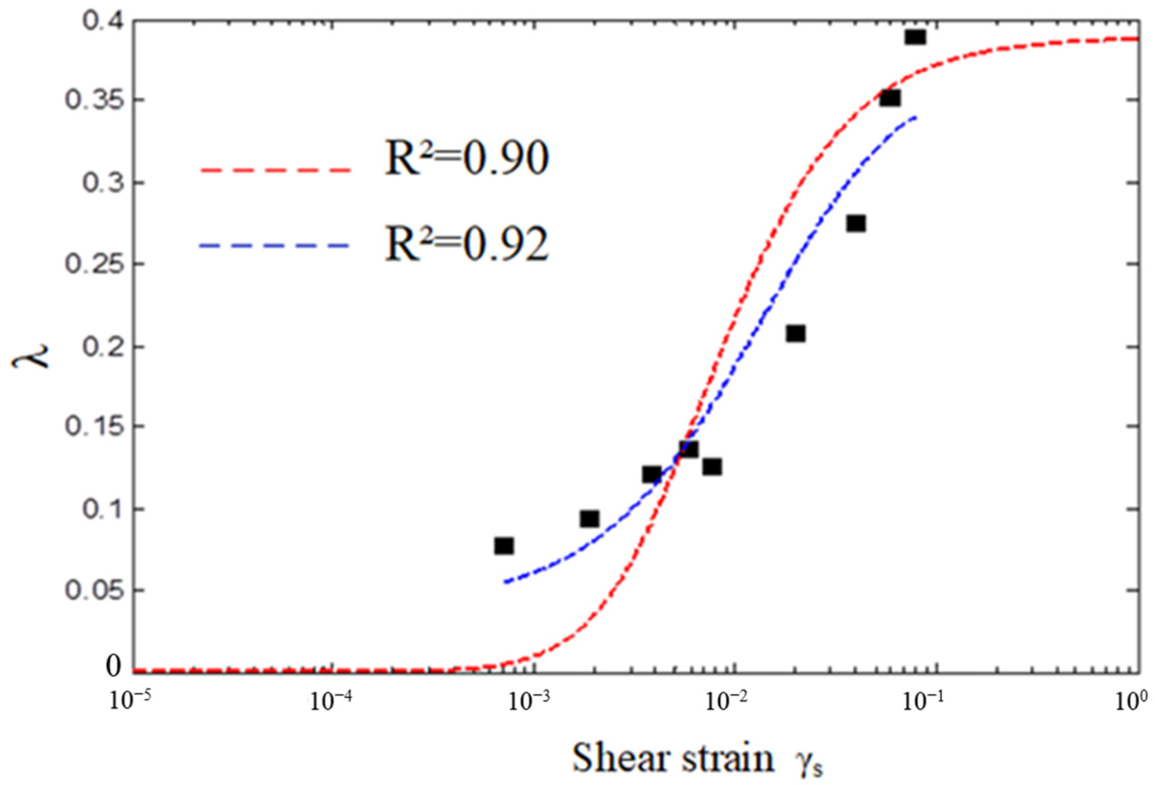
Under unloading conditions, such as excavation, the original stress state of the soil is disturbed to a certain extent, which is mainly due to a different degree of change in the soil structure. In situ soil has a maximum damping ratio of 0.227, whereas disturbed soil has a maximum damping ratio of 0.389. The change in the soil structure causes the value of the damping ratio to increase to different degrees compared with that of the in situ soil, which is reflected in the curve shape, where the damping ratios for the different shear strain amplitudes are uniformly distributed on the two sides of the curve (Figure 21). The dispersion of the curve fitting increases to some extent compared to the fitting results for the as-built soil. However, the three-parameter Davidenkov model can still reflect the law that the damping ratio of the disturbed soil changes corresponding to shear strain amplitude changes.

5. Influence of Strain History on Soil Dynamic Parameters

5.1. Analysis of Cyclic Loading Test Results

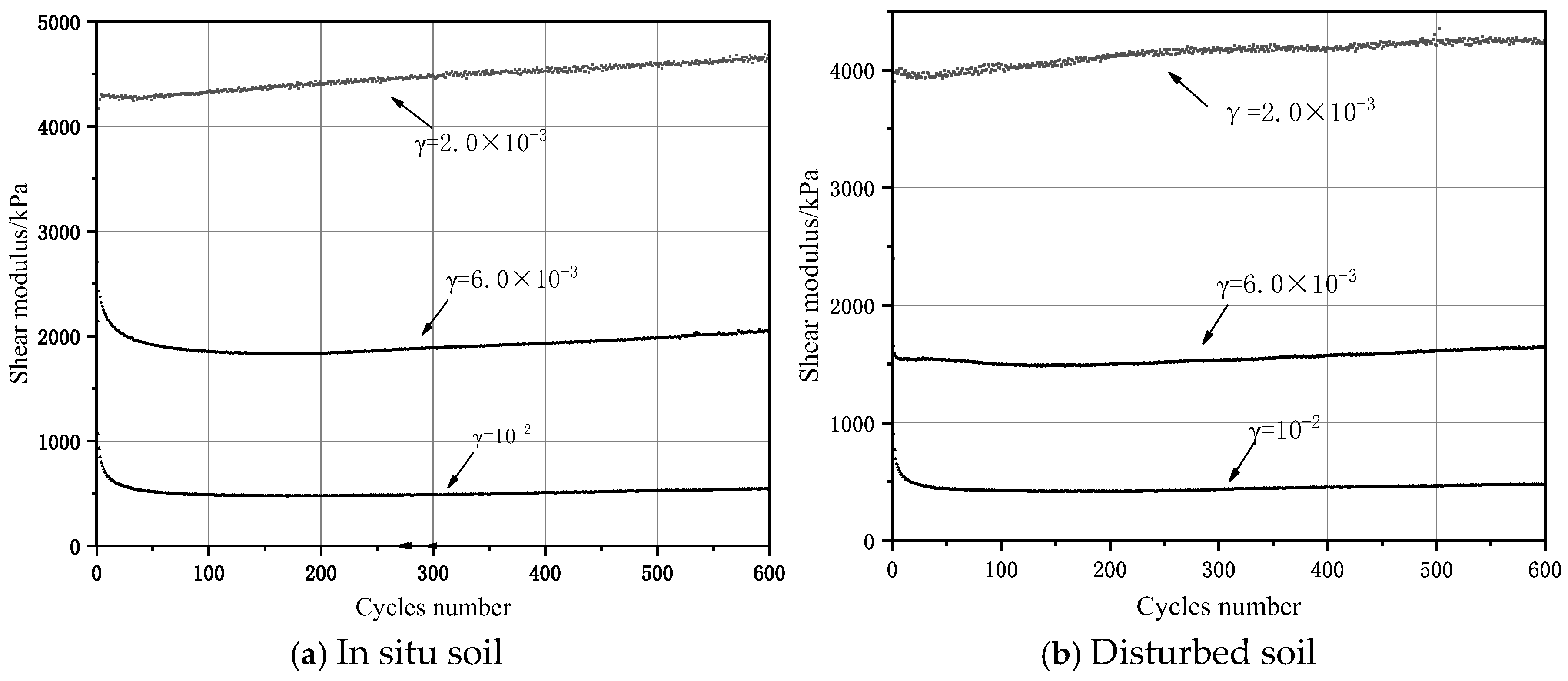
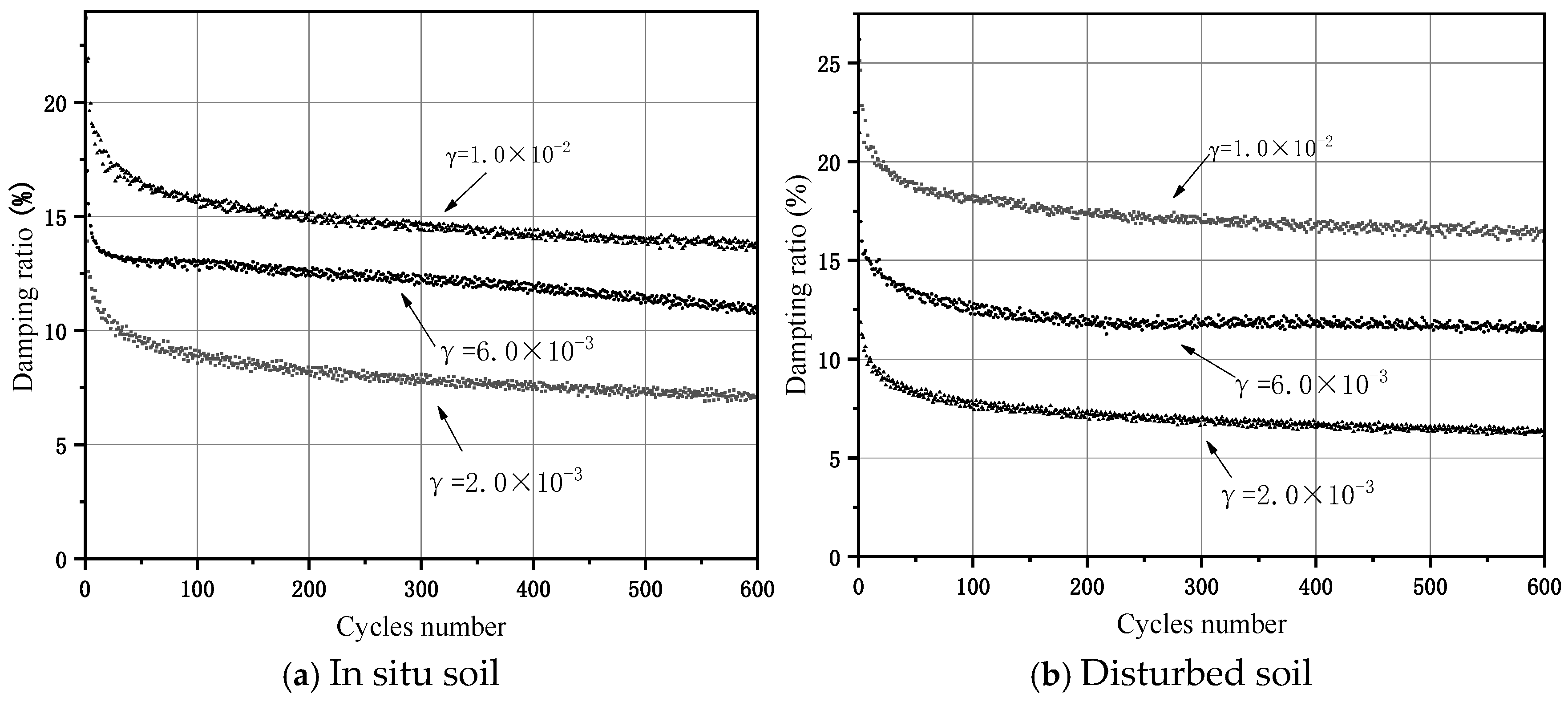
The cyclic loading method under a single amplitude, as introduced in Section 2 (Figure 6), was adopted. Figure 22 and Figure 23 show the dynamic shear modulus, as well as the damping ratio, with the cyclic loading number for the in situ and disturbed soils. The dynamic shear modulus versus the damping ratio was obtained statistically for each number of cyclic loadings.

As shown in Figure 22, when the shear strain is 1 × 10⁻², it is apparent that the shear modulus decreases more obviously in the first 50 weeks of the cycle, then changes slowly, and stabilizes after 100 cycles. When the shear strain is 6 × 10⁻³, the trend is the same as that of the shear strain 1 × 10⁻² for the first 50 cycles, then the shear modulus increases slowly after 100 cycles. When the shear variable is 2 × 10⁻³, the shear modulus increases with the cycle, and the trend is more obvious. Figure 23 shows that the damping ratio varies hyperbolically with the cycle period, and the damping ratio increases with increasing shear strain at a given cycle number. Similarly, the same rule applies to the disturbed soils.

With multiple cyclic loadings of equal amplitude, the shear modulus G diminishes, while the damping ratio D enhances with an increasing control strain γ in the same cyclic loading cycle. The dynamic shear modulus decreases with the increase in the cycle numbers for large strains. The damping ratio falls as the number of cycles grows under modest stresses, but the dynamic shear modulus rises with additional cycles. In the presence of significant stresses, the damping ratio falls as the number of cycles rises, and the dynamic shear modulus reduces initially, before gradually increasing.

5.2. The Effect of Strain History on the Soil Dynamic Shear Modulus and the Damping Ratio

It is evident from the aforementioned study that the loading history of the dynamic cycle affects the soil’s dynamic characteristics (dynamic shear modulus and damping ratio). For cohesive soils, this effect can be analyzed qualitatively and quantitatively by the physical parameter “cumulative body strain”, which varies with the loading history of the soil. Assuming that, for a certain soil, the initial dynamic characteristic curves are defined as the dynamic shear modulus curve and the damping ratio curve obtained when the cumulative body strain is 0, and are denoted as G_d⁰ and λ_d⁰, respectively. To create the dynamic shear modulus curve and damping ratio curve in the test to identify the cohesive soil’s dynamic characteristic curve, the values of G_d and λ_d, corresponding to the first effective hysteresis loop under each strain amplitude, are taken, which can be regarded as the initial dynamic characteristic curves. For the soil unit, one should take into account how the dynamic qualities of the current state are impacted by the prior cyclic strain history, and the initial dynamic characteristic curves should be corrected. Based on this purpose, two coefficients are introduced, denoted as C_G and C_λ, where C_G = G_d/G_d⁰ is the dynamic shear modulus strain accumulation coefficient, and C_λ = λ_d/λ_d⁰ is the damping ratio decay coefficient for strain accumulation. Here, G_d and λ_d are the dynamic shear modulus and the damping ratio in the current state after evaluating the impact of cumulative body strain, i.e., strain history, respectively. Obviously, G_d and λ_d are functions of the existing accumulated volume strain and the current dynamic shear strain amplitude.

Based on the above expressions, the following relational equations are established:

$$C_G=G_d/G_d^0$$

(18)

$$C_{\lambda }={\lambda }_d/{\lambda }_d^0$$

(19)

$$C_G=G_N/G_1$$

(20)

$${\lambda }_d={\lambda }_N/{\lambda }_1$$

(21)

In the above, G_N represents the dynamic shear modulus as the soil is subjected to cyclic tests, with the number of laps in the hysteresis curve being N. Similarly, λ_N is the damping ratio when the number of laps in the hysteresis curve is N.

Theoretically, the damping ratio, as well as the initial dynamic shear modulus, may be written as follows, according to the three-parameter Davidenkov model:

$$G_d^0({\gamma }_s)=G_{\max }\left\{1-{\left[{\displaystyle \frac{{\left(\frac{{\gamma }_s}{{\gamma }_0}\right)}^{2B}}{1+{\left(\frac{{\gamma }_s}{{\gamma }_0}\right)}^{2B}}}\right]}^A\right\}$$

(22)

$${\lambda }_d^0({\gamma }_s)={\lambda }_{\max }{\left[{\displaystyle \frac{{\left(\frac{{\gamma }_s}{{\gamma }_0}\right)}^{2B}}{1+{\left(\frac{{\gamma }_s}{{\gamma }_0}\right)}^{2B}}}\right]}^{A\beta }$$

(23)

Then, the mechanical coefficients of the dynamic properties (G_d and λ_d), considering the stress loading history (cumulative volumetric strain), can be expressed as:

$$G_d={C_G{G}_d}^0=C_G{G}_{\max }\left\{1-{\left[{\displaystyle \frac{{\left(\frac{{\gamma }_s}{{\gamma }_0}\right)}^{2B}}{1+{\left(\frac{{\gamma }_s}{{\gamma }_0}\right)}^{2B}}}\right]}^A\right\}=G_{d\max }^{\epsilon v}\left\{1-{\left[{\displaystyle \frac{{\left(\frac{{\gamma }_s}{{\gamma }_0}\right)}^{2B}}{1+{\left(\frac{{\gamma }_s}{{\gamma }_0}\right)}^{2B}}}\right]}^A\right\}$$

(24)

$${\lambda }_d={C_{\lambda }{\lambda }_d}^0=C_{\lambda }{\lambda }_{\max }{\left[{\displaystyle \frac{{\left(\frac{{\gamma }_s}{{\gamma }_0}\right)}^{2B}}{1+{\left(\frac{{\gamma }_s}{{\gamma }_0}\right)}^{2B}}}\right]}^{A\beta }={\lambda }_{d\max }^{\epsilon v}{\left[{\displaystyle \frac{{\left(\frac{{\gamma }_s}{{\gamma }_0}\right)}^{2B}}{1+{\left(\frac{{\gamma }_s}{{\gamma }_0}\right)}^{2B}}}\right]}^{A\beta }$$

(25)

The physical meanings of A, B, and β in the above equation are the same as in Section 3. To express the effect of stress loading history on the dynamic shear modulus, as well as the damping ratio, more clearly, the parameters ${\mathrm{G}}_{{\mathrm{d}}_{\mathrm{m}\mathrm{a}\mathrm{x}}}^{\mathsf{\epsilon }\mathrm{v}}$ and ${\mathsf{\lambda }}_{\mathrm{d}\mathrm{m}\mathrm{a}\mathrm{x}}^{\mathsf{\epsilon }\mathrm{v}}$ are introduced, and their expressions are given as:

$$G_{dmax}^{\epsilon v}=C_G{G}_{max}, {\lambda }_{dmax}^{\epsilon v}=C_{\lambda }{\lambda }_{max}$$

(26)

From Equation (26), it can be seen that the key to solving $G_{dmax}^{\epsilon v}$ and ${\lambda }_{dmax}^{\epsilon v}$ is to obtain C_G and C_λ. The values of C_G and C_λ can be obtained by comparing the theoretical calculations with the test results in the following section.

From Equation (26), it can be seen that the influence of cyclic loading history on mechanical parameters is mainly reflected in the change in cumulative volumetric strain, and in the test, for various shear strain amplitudes, the link between the cyclic loading number and the dynamic shear modulus, as well as the damping ratio, can be intuitively determined. Then, to study the theoretical connection between dynamic shear modulus, as well as the damping ratio, and the accumulated volumetric strain, the calculation method for the accumulated volumetric strain needs to be clarified, which requires the establishment of the cyclic load number N and the cumulative volumetric strain have a functional connection. The relationship between the accumulated volumetric strain and N can be established in the test. In the cyclic shear test, the copper ring is used to limit the deformation of the soil specimen, so that the specimen’s volumetric strain can be ignored in the deformation of the soil in the direction of the cross-section. It is considered that only axial strain is caused by the volumetric strain of the soil specimen.

In the soil cyclic single-shear test, after the completion of the first cyclic loading at a certain strain amplitude, the axial (volumetric) strain can be expressed as:

$${\displaystyle \frac{\Delta h_1}{20}}={\epsilon }_a$$

(27)

where $\Delta {\mathrm{h}}_1$ is the amount of change in how the specimen is oriented axially after the completion of the first cyclic loading; the height of the specimen in the cyclic single-shear test is 20 mm. In the following part, the amount of change in the axial direction of the soil body after the completion of the nth loading is expressed by $\Delta h_n$.

After the second cycle of loading is completed, the expression for the axial (volumetric) strain is:

$${\displaystyle \frac{\Delta h_2}{20-\Delta h_1}}={\epsilon }_a$$

(28)

After the completion of the third cycle of loading, the expression for the axial (volumetric) strain is:

$${\displaystyle \frac{\Delta h_3}{20-\Delta h_1-\Delta h_2}}={\epsilon }_a$$

(29)

The expression for the axial (volumetric) strain after the completion of the nth cycle of loading is:

$${\displaystyle \frac{\Delta h_n}{20-\Delta h_1-\Delta h_2-\dots -\Delta h_{n-1}}}={\epsilon }_a$$

(30)

In the above:

$${\epsilon }_a={\displaystyle \frac{{\gamma }_s}{1+\mu }}$$

(31)

γ_s is the shear strain amplitude. In this test, three multi-week cyclic shear tests under shear strain amplitude were carried out; γ_s takes the values of 2 × 10⁻³, 6 × 10⁻³, and 1 × 10⁻²; and μ is the Poisson’s ratio, which is taken as 0.45, according to Ref. [38].

After the completion of the nth cyclic loading, the cumulative body strain $\mathsf{\epsilon }\mathrm{v}$ (axial deformation/initial height of the specimen), is expressed as:

$${\epsilon }_V={\displaystyle \frac{\Delta h_1+\Delta h_2+\dots +\Delta h_{n-1}+\Delta h_n}{20}}$$

(32)

The relationship between the cumulative volumetric strain and the number of cyclic loading n can be obtained by bringing the expressions $\Delta h_1$, $\Delta h_2$ …… $\Delta h_n$, etc., into the expression of ${\epsilon }_V$, in turn:

$$\mathrm{Let} {\displaystyle \sum _{i=1}^n\Delta h_i}=\Delta h_1+\Delta h_2+\dots +\Delta h_{n-1}+\Delta h_n; 600\ge n\ge 2$$

(33)

Further, iterative calculations can be obtained as:

$$\begin{array}{l}{\displaystyle \sum _{i=1}^n\Delta h_i}=\Delta h_1+\Delta h_2+\dots +\Delta h_{n-1}+(20-\Delta h_1-\Delta h_2-\dots -\Delta h_{n-1}){\epsilon }_a\\ =(1-{\epsilon }_a)(\Delta h_1+\Delta h_2+\dots +\Delta h_{n-1})+20{\epsilon }_a\\ =(1-{\epsilon }_a)\left[\Delta h_1+\Delta h_2+\dots +\Delta h_{n-2}+(20-\Delta h_1-\Delta h_2-\dots -\Delta h_{n-2}){\epsilon }_a\right]+20{\epsilon }_a\\ = (1-{\epsilon }_a)\left[(1-{\epsilon }_a)(\Delta h_1+\Delta h_2+\dots +\Delta h_{n-2})+20{\epsilon }_a\right]+20{\epsilon }_a\\ ={(1-{\epsilon }_a)}^2(\Delta h_1+\Delta h_2+\dots +\Delta h_{n-2})+20{\epsilon }_a(1-{\epsilon }_a)+20{\epsilon }_a\\ ={(1-{\epsilon }_a)}^3(\Delta h_1+\Delta h_2+\dots +\Delta h_{n-3})+20{\epsilon }_a{(1-{\epsilon }_a)}^2+20{\epsilon }_a(1-{\epsilon }_a)+20{\epsilon }_a\\ =\dots \dots \\ ={(1-{\epsilon }_a)}^{n-1}\Delta h_1+20{\epsilon }_a{(1-{\epsilon }_a)}^{n-2}+20{\epsilon }_a{(1-{\epsilon }_a)}^{n-3}+\dots +20{\epsilon }_a\\ ={\displaystyle \frac{20{\epsilon }_a\left[1-{(1-{\epsilon }_a)}^n\right]}{1-{\epsilon }_a}}\end{array}$$

(34)

And then there is

$${\epsilon }_V={\displaystyle \frac{{\epsilon }_a\left[1-{(1-{\epsilon }_a)}^n\right]}{1-{\epsilon }_a}}(2\le n\le 600)$$

(35)

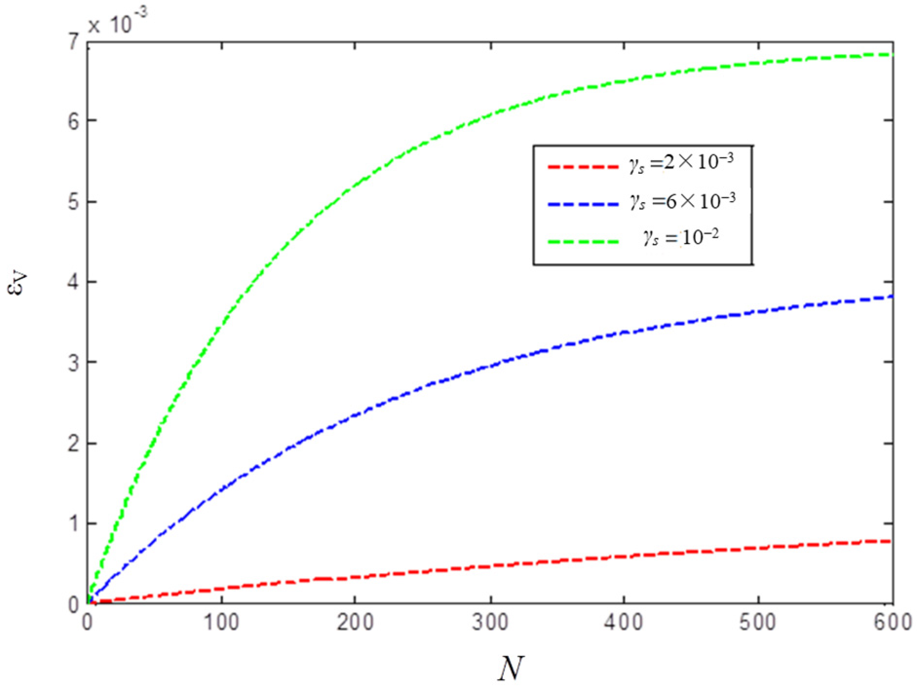
From the above equation, it can be seen that after n times of cyclic loading, the cumulative volumetric strain ${\mathsf{\epsilon }}_{\mathrm{V}}$ is a result of εa and the number of times of loading n. Figure 24 illustrates the connection between the total volumetric strain and the number of cyclic loading N.

From Figure 24, it is evident that at each shear strain amplitude (small, medium, and large shear strains), the amplitude of the increase in volumetric strain ε_v reduces with the increase in the number of cycles N. This phenomenon can be primarily attributed to the nature of the soil as a three-phase body. As N increases, the soil particle distribution gradually densifies, making further densification under the same shear strain amplitude increasingly challenging. Additionally, it is observed that with the increase in dynamic shear strain amplitude, the volumetric strain exhibits more pronounced growth with the increasing number of loadings.

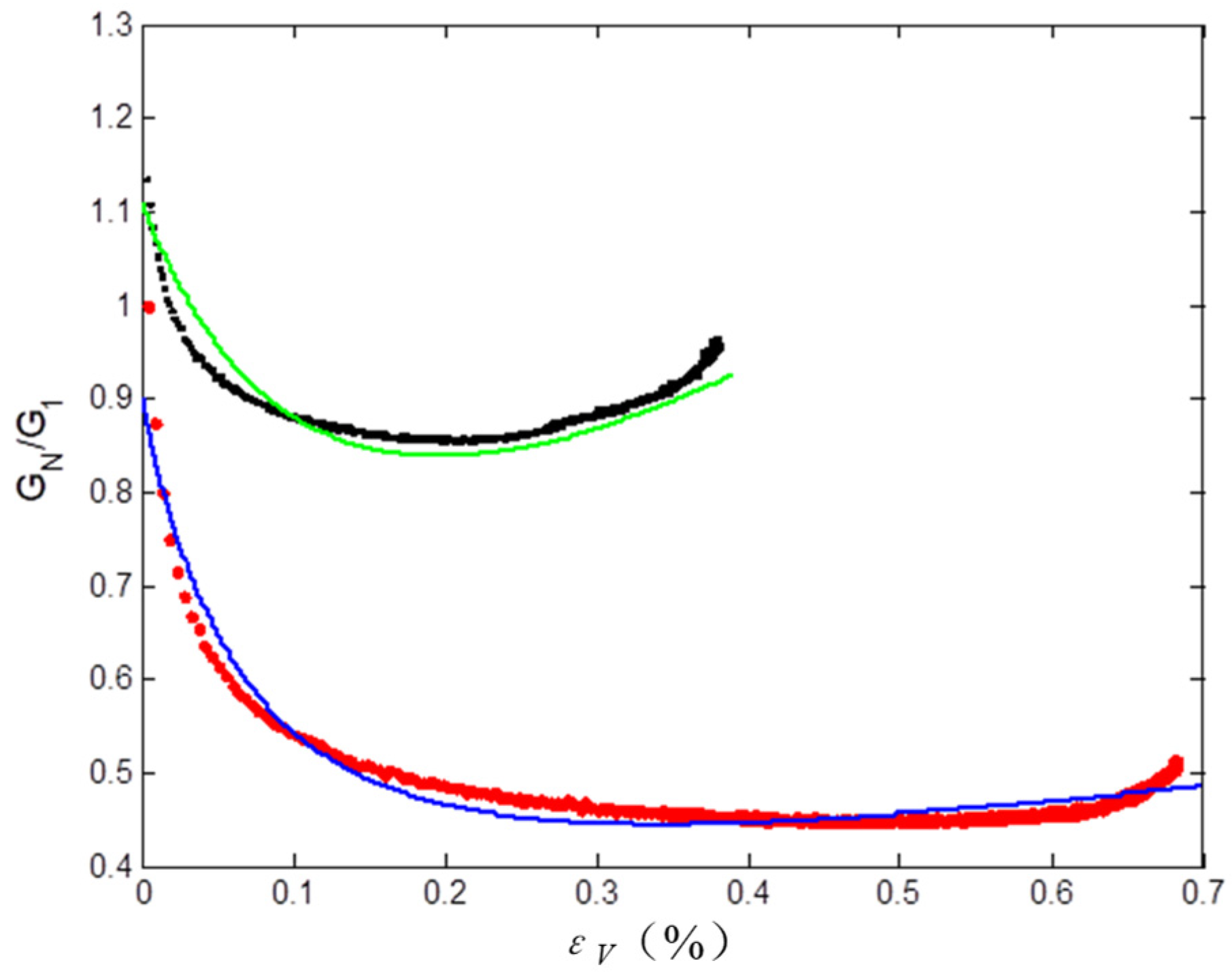
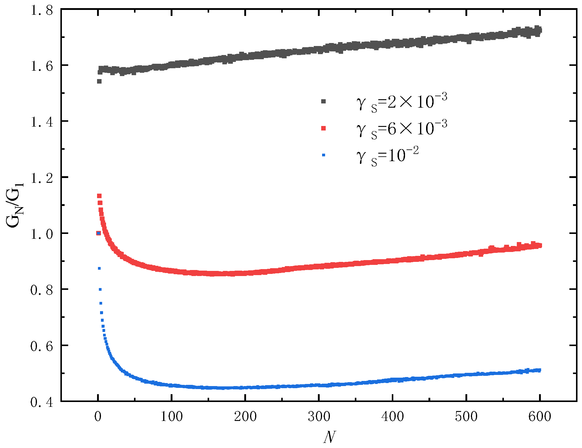
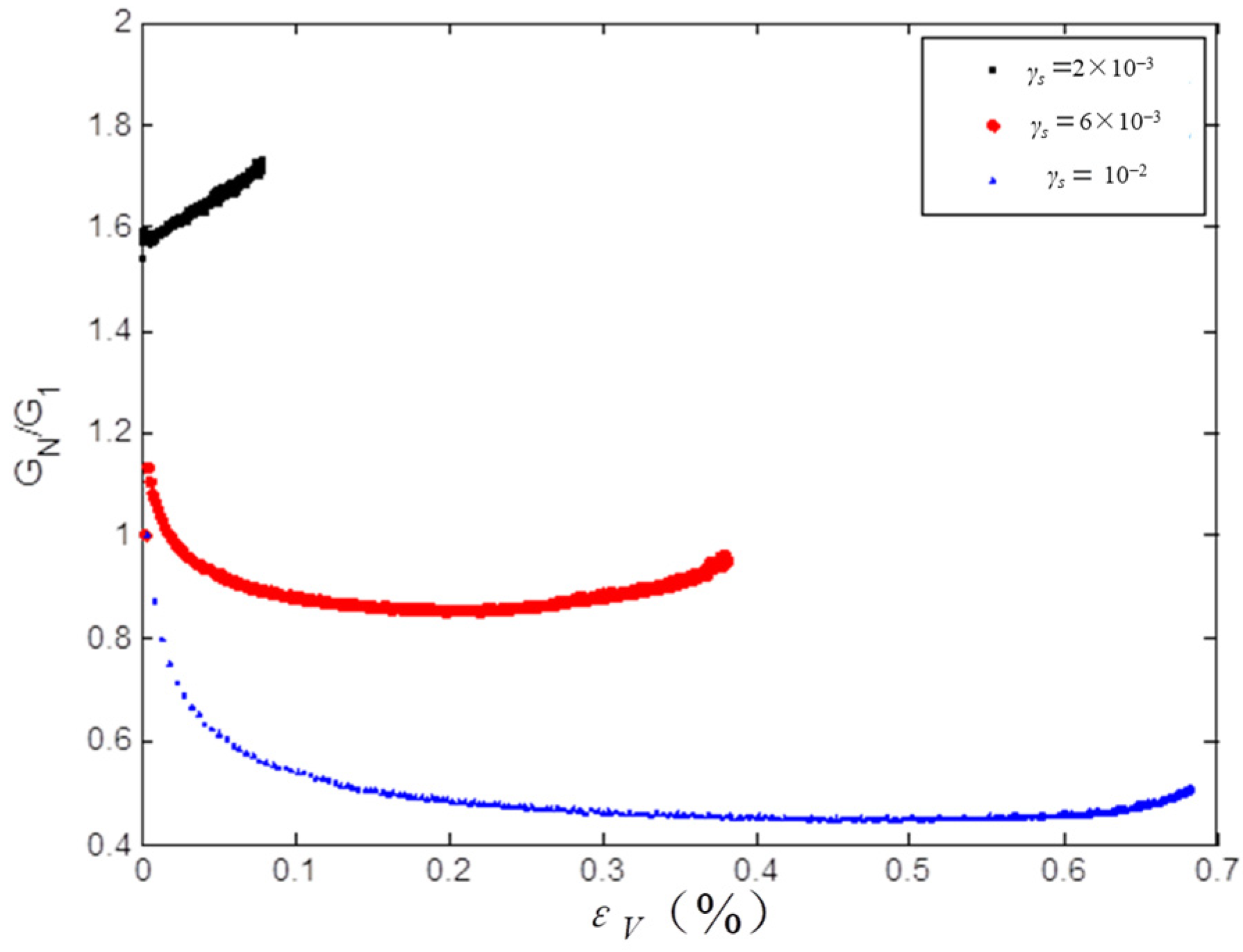
The relationship between the normalized dynamic shear modulus (G_N/G₁) and the number of cycles N is shown in Figure 25. When the shear strain amplitude is small (2 × 10⁻³), the normalized dynamic shear modulus increases rapidly and then changes smoothly in the first few cycles. As the shear strain amplitude increases, the dynamic shear modulus exhibits a downward trend that is followed by a smooth change, and the extent of the dynamic shear modulus reduction increases with the shear strain amplitude.

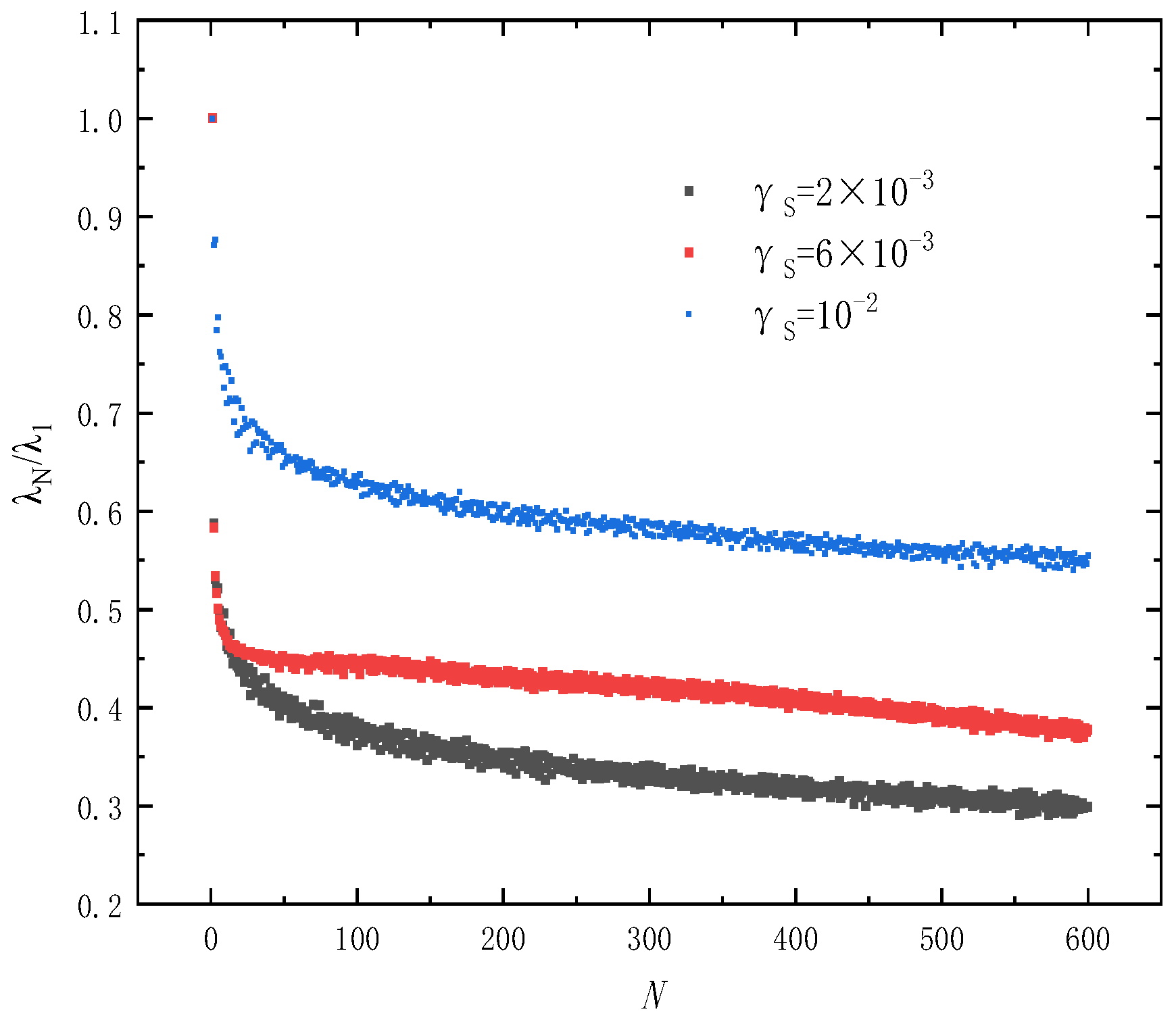
Figure 26 shows the relationship between the normalized damping ratio (λ_N/λ₁) and the number of cycles N. As the cycle number increases, the decay of the damping ratio follows a pattern of initial rapid change, followed by a gradual slowdown. When N is greater than 300, the change in the normalized damping ratio tends to stabilize. With the same number of loops loaded, the larger the shear strain amplitude, the larger the normalized damping ratio value.

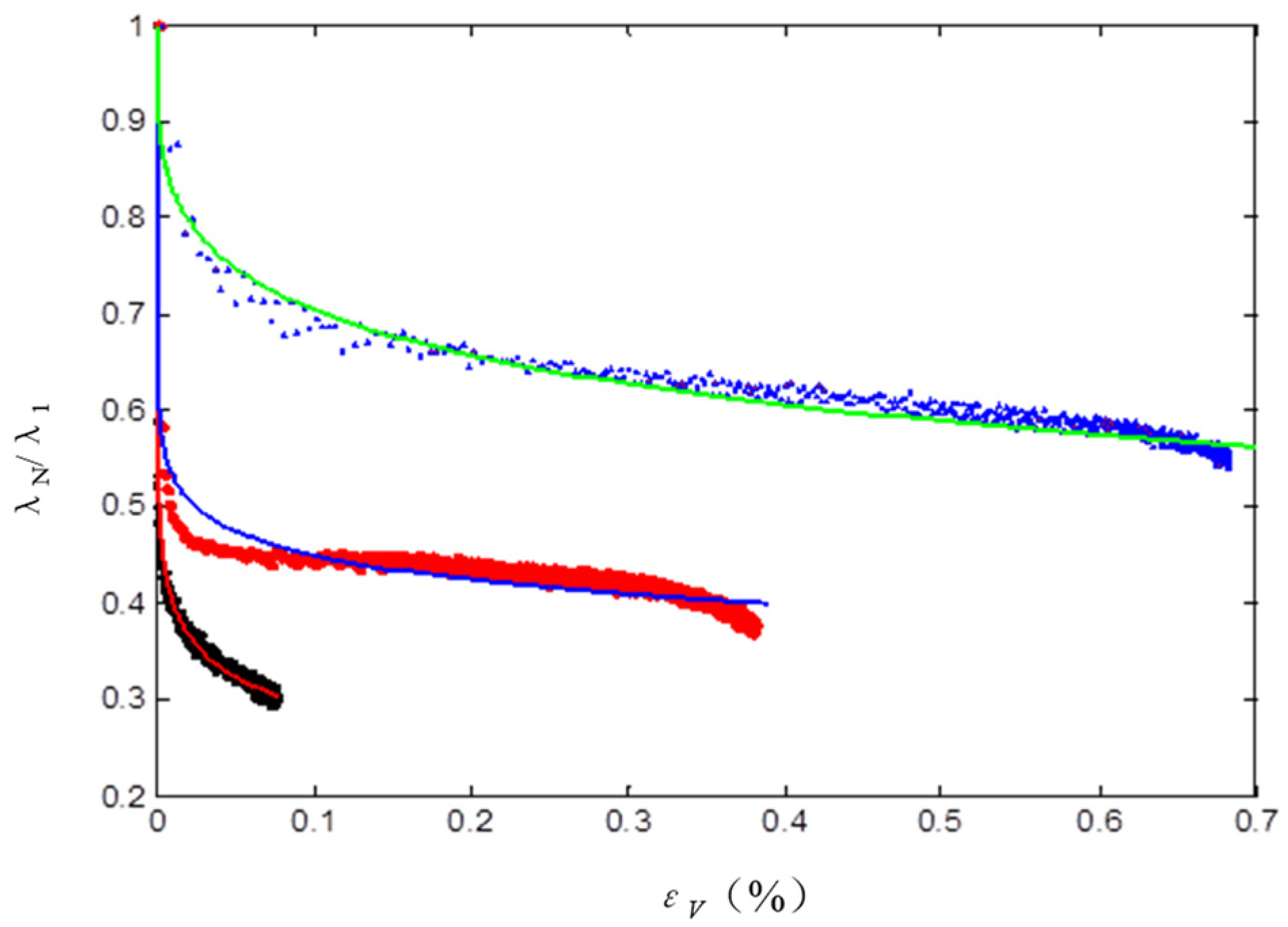
Equation (35) establishes the relationship ε_V between the number of cycles N and the volumetric strain, from which the accumulated volumetric strain can be calculated. The connection, in Figure 26, between N and the standardized dynamical modulus of shear can then be transformed into the relationship between the normalized dynamic shear modulus and the accumulated volumetric strain, as shown in Figure 27.

Based on the trend in the test results, this paper proposes the following dimensionless shear modulus as a function of volumetric strain for different shear strain amplitudes (γ_s = 2 × 10⁻³ for small strains, and γ_s = 6 × 10⁻³, 1 × 10⁻² for medium and high strains):

$$\left\{\begin{array}{lll}{\displaystyle \frac{G_N}{G_1}}={\displaystyle \frac{b\left[1-{\left(1-{\epsilon }_y\right)}^a\right]}{1-{\epsilon }_y}} & {\gamma }_s=2\times {10}^{-3}& \\ {\displaystyle \frac{G_N}{G_1}}=c{\left({\epsilon }_y-f\right)}^e+d\left({\epsilon }_y-f\right)& {\gamma }_s=6\times {10}^{-3},{10}^{-2}& \end{array}\right.$$

(36)

where G₁ is the dynamic shear modulus at the first hysteretic loop at a certain shear strain amplitude, i.e., the dynamic shear modulus when the cumulative strain is 0. G_N is the dynamic shear modulus at the Nth loop. a, b, c, d, e, and f are the test parameters, which can be obtained by fitting, according to the test data.

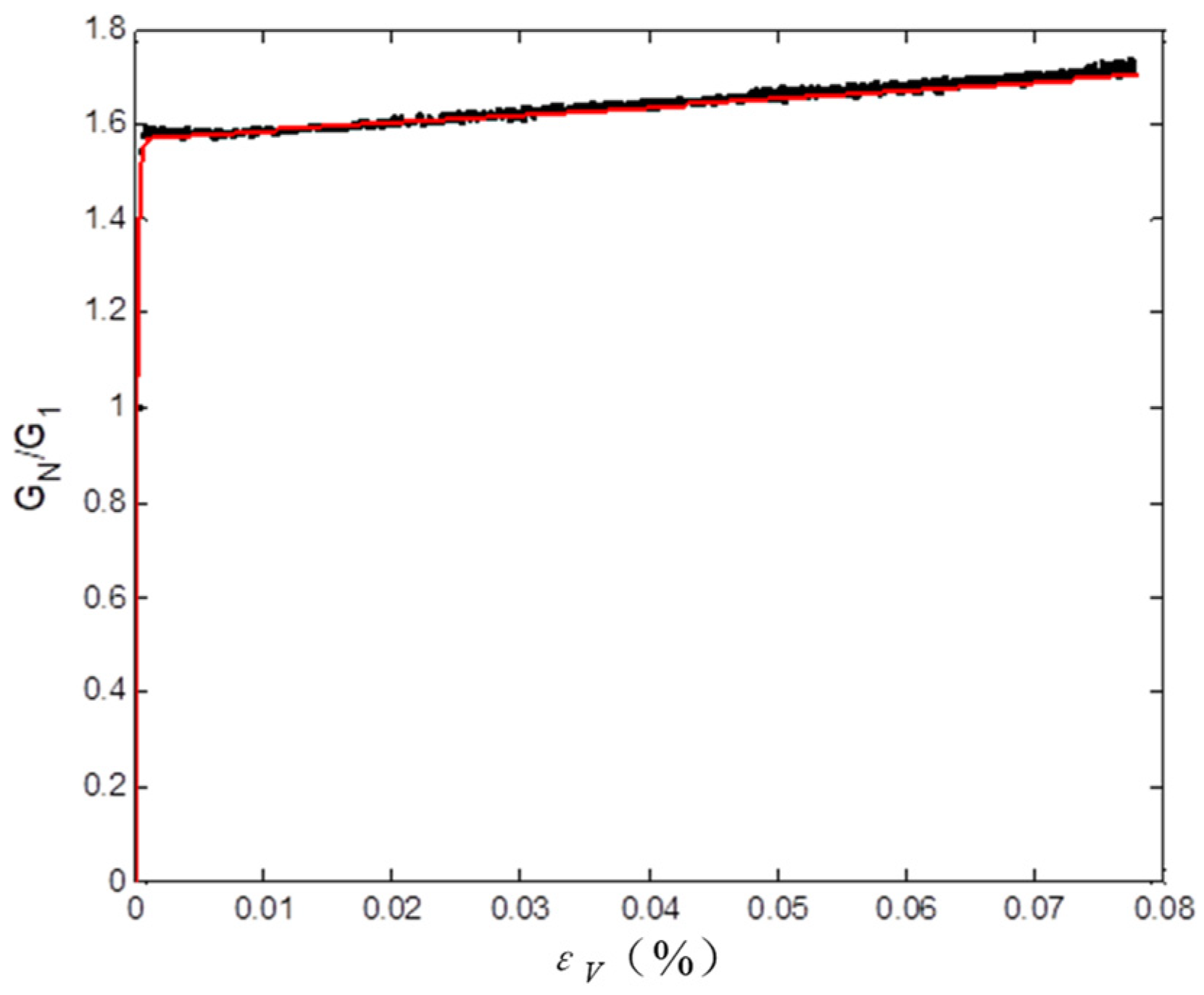
The test curve and the fitted curve according to the theoretical formula are represented in the same figure, as shown in Figure 28 and Figure 29. It can be seen that the theoretical curve and the test data fit well, and the theoretical curve can better respond to the change rule for the test data. The theoretical curve expression after determining the test parameters is:

$$\begin{array}{ll}& {\displaystyle \frac{G_N}{G_1}}={\displaystyle \frac{1.57\left[1-{\left(1-{\epsilon }_y\right)}^{{6.1\times 10}^3}\right]}{1-{\epsilon }_y}} {\gamma }_s=2\times {10}^{-3}\\ & {\displaystyle \frac{G_N}{G_1}}=1.21{\left({\epsilon }_y+0.1796\right)}^{1.167}+0.17/\left({\epsilon }_y+0.1796\right) {\gamma }_s=6\times {10}^{-3}\\ & {\displaystyle \frac{G_N}{G_1}}=0.456{\left({\epsilon }_y+0.086\right)}^{0.54}+0.067/\left({\epsilon }_y+0.086\right) {\gamma }_s=1\times {10}^{-2}\end{array}$$

(37)

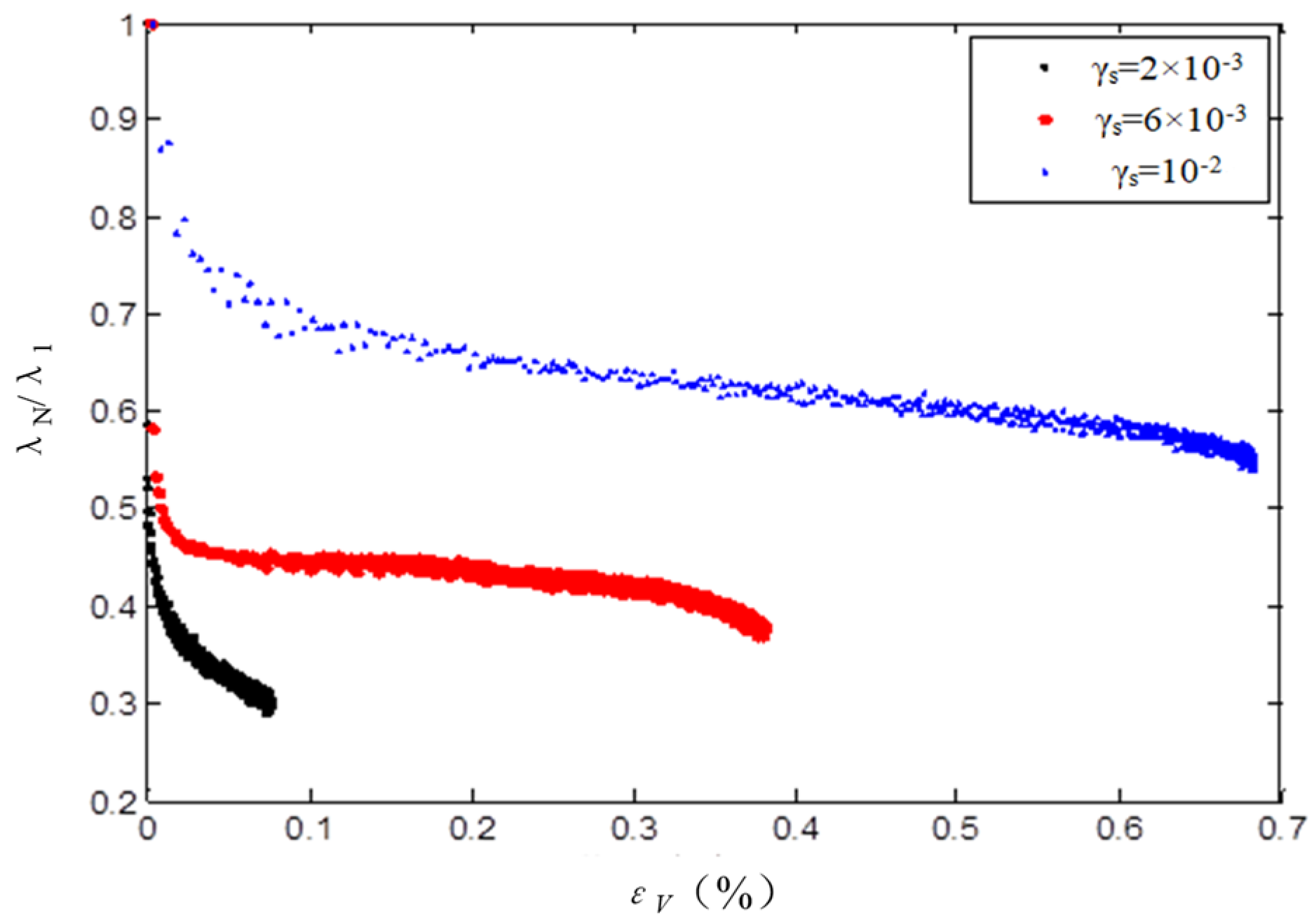
A schematic diagram of the normalized damping ratio versus strain accumulation is shown in Figure 30. The theoretical curve of the damping ratio decay change versus the volumetric strain takes the following form:

$${\displaystyle \frac{{\lambda }_N}{{\lambda }_1}}={\displaystyle \frac{1}{1+{\left(\alpha {\xi }_V\right)}^{A+B{\gamma }_0}}}$$

(38)

In the above equation, λ_N is the damping ratio at the Nth lap; λ1 is the damping ratio at the 1st lap; and α, A, and B are the fitting parameters. Figure 31 shows the contrast between the theoretical curve and the test curve. As can be seen from Figure 31, the theoretical curve fits well with the test results. The relationship between the normalized damping ratio and the cumulative volumetric strain, which is consistent with the data in this test, is given by

$$\begin{array}{l}{\displaystyle \frac{{\lambda }_N}{{\lambda }_1}}=1/\left(1+{\left(562.1\times x\right)}^{\left(-0.0066 + 115.26 \times 2 \times {10}^{-3}\right)}\right) {\gamma }_s=2\times {10}^{-3}\\ {\displaystyle \frac{{\lambda }_N}{{\lambda }_1}}=1/\left({1+(38.93\times x)}^{\left(0.373 - 37.38 \times 6 \times {10}^{-3}\right)}\right) {\gamma }_s=6\times {10}^{-3}\\ {\displaystyle \frac{{\lambda }_N}{{\lambda }_1}}=1/\left({1+(0.65\times x)}^{\left(0.29 - 2.87 \times {10}^{-2}\right)}\right) {\gamma }_s={10}^{-2}\end{array}$$

(39)

The expressions C_G and C_λ are determined from Equations (37) and (39), and in the above we mentioned that:

$$G_{d\max }^{\epsilon v}=C_G{G}_{\max }\hspace{1em}{\lambda }_{d\max }^{\epsilon v}=C_{\lambda }{\lambda }_{\max }$$

(40)

From the above analysis, the dynamic shear modulus and the damping ratio, considering the cumulative volumetric strain, can be calculated by substituting C_G = G_N/G₁ and C_λ = λ_N/λ₁ for different shear strain amplitudes into the above equation. According to this method, the expression of the law that influences the action of dynamic loads, such as seismic loads, on the dynamic soil characteristics, considering the actions of the installation history (volumetric strain), has been realized.

6. Discussion

The soil investigated in this study is a cohesive silty clay from Changsha, southern China, characterized by 16–23% clay-sized particles, plasticity indexes of 11.7–16.5, and liquidity indexes of 0.22–0.68, classifying it as low- to medium-plasticity clay in a plastic to semi-solid state. The critical distinction between in situ and disturbed samples lies in the preservation of natural fabric—including particle orientation, aggregation, and interparticle cementation—which fundamentally controls mechanical response. In situ soils carry load through inter-particle surface forces (van der Waals attractions, electrical double-layer interactions, and cementation bonds) operating within a structured fabric, resulting in significantly higher dynamic shear moduli (up to 5912 kPa at small strains) compared to disturbed soils (4975 kPa). This structural contribution persists until shear strains exceed critical thresholds that cause bond breakage and fabric destruction.

Deformation in cohesive soils evolves through distinct mechanisms with increasing strain amplitude. At very small strains (γ < 10⁻³), deformation is primarily elastic and recoverable, producing elliptical hysteresis loops with minimal energy dissipation. As strain increases into the intermediate range (10⁻³ to 10⁻²), plastic deformation develops at particle contacts, and hysteresis loops deviate from an elliptical shape. At large strains (γ > 2 × 10⁻² for the in situ soil, and γ > 8 × 10⁻³ for the disturbed soil), hysteresis curves develop a characteristic “S-shape”, reflecting progressive structure breakdown and particle realignment. Water profoundly influences all aspects of behavior: adsorbed water layers transmit inter-particle forces and provide cohesive strength; pore pressure development under undrained cycling reduces effective stress, causing modulus degradation; and the water content relative to the plastic limit (liquidity index) fundamentally controls stiffness, with higher liquidity indexes consistently yielding lower dynamic shear moduli across all strain amplitudes.

Under cyclic loading, cohesive soils exhibit nonlinear stress–strain relationships, with hysteresis and degradation well-described by the three-parameter Davidenkov model. The damping ratio increases from 5 to 8% at small strains, to 22 to 38% at γ = 8 × 10⁻², reflecting enhanced energy dissipation through plastic and viscous mechanisms. Critically, behavior exhibits strong dependence on strain history: at small strains (γ = 2 × 10⁻³), continued cycling increases the modulus and decreases damping through densification; at large strains (γ = 1 × 10⁻²), the modulus decreases initially due to pore pressure buildup and structure degradation before stabilizing. This study introduced volumetric strain ε_v as a state variable capturing integrated strain history, enabling quantification of history effects through coefficients C_G and C_λ. The relationship between the normalized modulus and accumulated volumetric strain demonstrates that property evolution correlates strongly with cumulative deformation, providing a rational framework for incorporating strain history effects into seismic site response analysis.

Since the specimens were unsaturated, the accumulation of pore water pressure was limited during undrained cyclic shearing, resulting in a smaller increase in pore pressure. In turn, this mitigated the effect of effective stress reduction on modulus degradation. This partially explains why no significant modulus degradation was observed under high strains in this experiment, as well as why disturbed soil exhibited stable modulus behavior despite structural failure. Undisturbed soil, due to the presence of its natural structure, has a higher initial modulus; however, structural failure is pronounced under high strains, resulting in the appearance of an “S-shaped” hysteresis curve earlier than in disturbed soil. Disturbed soil, due to partial structural failure, has a lower initial modulus; however, its modulus variation pattern, influenced by loading history, is more gradual. The differences between the two are not only attributable to structural state but also related to variations in moisture distribution and the matrix’s ability to maintain cohesion under unsaturated conditions.

The parameter sensitivity analysis in Section 4.2 (Figure 10, Figure 11, Figure 12 and Figure 13) shows that parameters A, B, and γ₀ in the Davidenkov model independently control distinct features of the modulus degradation and damping ratio curves. Beyond their mathematical roles, these parameters exhibit systematic correlations with key soil physical properties. As shown in Table 1, Table 2, Table 3 and Table 4, in the situ soils (I_p = 12.9–16.5, I_L = 0.35–0.43) yield fitted parameters of A = 2.62, B = 0.45, and γ₀ = 22.4 × 10⁻⁴, whereas the disturbed soils (I_p = 11.7–13.3, I_L = 0.42–0.68) give A = 1.43, B = 0.58, and γ₀ = 35.4 × 10⁻⁴. The reduction in A and increase in γ₀ for the disturbed soils reflect the breakdown of natural cementation and fabric rearrangement. Parameter B correlates positively with I_p, indicating that higher plasticity results in a more gradual nonlinear transition due to enhanced viscous interparticle interactions. The reference strain γ₀ correlates positively with I_L and porosity e, as looser or wetter soils delay the onset of stiffness degradation. These correlations demonstrate that A, B, and γ₀ are not purely empirical but are intrinsically linked to soil fabric, stress history, and moisture sensitivity, enabling more rational parameter selection for cohesive soils with varying plasticity and disturbance levels.

It should be noted that Equations (37) and (39) are empirical relationships derived from cyclic single-shear tests on Changsha cohesive soil under specific conditions. The constants in these equations (e.g., α, A, and B) are dependent on soil type, confining pressure, and loading characteristics. For instance, soils with higher plasticity or different mineral compositions may exhibit distinct relationships between the normalized dynamic shear modulus and accumulated volumetric strain. Similarly, variations in confining stress and loading frequency can alter the rate of modulus degradation and damping evolution. Therefore, when applying the proposed model to other engineering scenarios, such as different soil types and stress levels, the empirical constants should be recalibrated based on corresponding cyclic test data. The primary contribution of this study lies in establishing a framework that incorporates strain history effects via accumulated volumetric strain, rather than providing universally fixed parameters. Future work should focus on extending this framework to a broader range of soils and loading conditions to validate and generalize the proposed approach.

7. Conclusions

This study investigated the nonlinear mechanical behavior of Changsha cohesive soil through cyclic shear testing, comparing in situ and disturbed specimens across multiple strain amplitudes to quantify how strain history influences dynamic properties. The experimental results demonstrate that cohesive soil behavior is fundamentally nonlinear and history-dependent: for in situ soil, dynamic shear modulus decreases from approximately 5900 kPa at small strains to 630 kPa at γ = 8 × 10⁻², while the damping ratio increases correspondingly from 5.6% to 22.7%. Hysteresis curves evolve from elliptical shapes at small strains to distinctly “S-shaped” configurations at large strains (γ > 2 × 10⁻² for the in situ soil, and γ > 8 × 10⁻³ for the disturbed soil), indicating progressive breakdown of the natural structure. The disturbed soils exhibit a consistently lower modulus and higher damping across all strain amplitudes, directly demonstrating the contribution of natural fabric to mechanical stiffness.

The three-parameter Davidenkov model effectively captures the relationship between shear strain and normalized dynamic shear modulus, with fitted parameters of A = 2.62, B = 0.45, and γ₀ = 22.4 × 10⁻⁴ for the in situ soil, and A = 1.43, B = 0.58, and γ₀ = 35.4 × 10⁻⁴ for the disturbed soil. Within the seismic shear strain range of 2 × 10⁻⁴ to 2 × 10⁻³, the model shows excellent agreement with the experimental data. Parameter sensitivity analysis reveals that B controls curve curvature, A influences vertical shifting, and γ₀ represents the reference strain around which degradation is most rapid. The damping ratio follows a related functional form, with an additional parameter β, yielding values of 0.54 for the in situ soil and 1.86 for the disturbed soil.

A key contribution is the quantification of strain history effects through cumulative volumetric strain ${\epsilon }_V$, with the relationship ${\epsilon }_V={\displaystyle \frac{{\epsilon }_a\left[1-{(1-{\epsilon }_a)}^n\right]}{1-{\epsilon }_a}}$ established between accumulated strain and loading cycles. To more clearly articulate the impact of stress loading history on the dynamic shear modulus and damping ratio, $G_{d\max }^{\epsilon v}$ and ${\lambda }_{d\max }^{\epsilon v}$, which are considered volumetric strains, are introduced. Additionally, coefficients for calculating the damping ratio and shear modulus are incorporated, leading to the establishment of the following formulas: $G_{d\max }^{\epsilon v}=C_G{G}_{\max }$ and ${\lambda }_{d\max }^{\epsilon v}=C_{\lambda }{\lambda }_{\max }$. Based on the cyclic single-shear test data, the theoretical formulas of C_G and C_λ were obtained for different shear strain amplitudes, and then the theoretical formulas of dynamic shear modulus and damping ratio were obtained considering the stress loading history. This study provides a rational framework for updating soil properties during seismic events, though validation under multi-directional loading and for broader soil types remains necessary for general application in the future.

References

1. Wang, J.; Yao, L.; Jiang, L. Damage mode and mechanism of soil deformation under earthquake. J. Southwest Jiaotong Univ. 2010, 45, 196–202. (In Chinese) [Google Scholar]
2. Fan, C.; Zhang, W.; Lai, Y.; Wang, B. Mechanical behaviors of frozen clay under dynamic cyclic loadings with freeze-thaw cycles. Cold Reg. Sci. Technol. 2021, 181, 103184. [Google Scholar] [CrossRef] [Scilit]
3. Liu, P.H.; Fang, H.G.; Song, L.J. Experimental Investigation for Structural Effect of Soft Clay under Low Frequency Cyclic Loading. Appl. Mech. Mater. 2013, 438–439, 673–676. [Google Scholar] [CrossRef] [Scilit]
4. Si, J.; Liu, S.; Zhang, H.; Zhu, Y.; Zheng, Y. Failure investigation and treatments of tunnel entrance collapse in weak diatomaceous soil induced by heavy rainfall through coupled surface and groundwater flows. Eng. Fail. Anal. 2023, 150, 107337. [Google Scholar] [CrossRef] [Scilit]
5. Lei, J.; Liu, C.; Li, F.; Sun, L. A united hardening rule considering monotonic and cyclic strength degradation of clay. Soil Dyn. Earthq. Eng. 2023, 166, 107754. [Google Scholar] [CrossRef] [Scilit]
6. Zhang, S.; Cheng, X.; Zhou, X.; Sun, Y. Face stability analysis of large-diameter underwater shield tunnel in soft-hard uneven strata under fluid-solid coupling. Geomech. Eng. 2023, 253, 111283. [Google Scholar]
7. Shiran, A.M.P. Effects of the constitutive relationship on seismic response of soils. part I. Const. Model. Cycl. Behav. Soils Soil Dyn. Earthq. Eng. 2000, 19, 305–318. [Google Scholar]
8. Yang, L.; Han, Z.; Guo, C.; Cao, D.; Ni, P.; Wang, F. An innovative solution for the dynamic response of buried pipelines in layered transversely isotropic soil under pavement structures. Comput. Geotech. 2022, 143, 104602. [Google Scholar] [CrossRef] [Scilit]
9. Wang, Y.; Stokoe, K.H.I.I.I. Development of Constitutive Models for Linear and Nonlinear Shear Modulus and Material Damping Ratio of Uncemented Soils. J. Geotech. Geoenviron. Eng. 2022, 148, 04021192. [Google Scholar] [CrossRef] [Scilit]
10. Yan, Z.; Kai, Z.; Yanjv, P.; Guoxing, C. Dynamic shear modulus and damping ratio characteristics of undisturbed marine soils in the Bohai Sea, China. Earthq. Eng. Eng. Vib. 2022, 21, 297–312. [Google Scholar] [CrossRef] [Scilit]
11. Cui, G.; Zhu, C.; Xi, C.; Ma, S.; Liu, Z.; Zhang, D. Experimental study of the dynamic characteristics of Songhua River silt with fine grains under freeze-thaw cycles using asymmetric hysteresis. Cold Reg. Sci. Technol. 2022, 196, 103511. [Google Scholar] [CrossRef] [Scilit]
12. Zhang, W.; Seylabi, E.E.; Taciroglu, E. Validation of a three-dimensional constitutive model for nonlinear site response and soil-structure interaction analyses using centrifuge test data. Int. J. Numer. Anal. Methods Geomech. 2017, 41, 1828–1847. [Google Scholar] [CrossRef] [Scilit]
13. Borja, R.I.; Amies, A.P. Multiaxial Cyclic Plasticity Model for Clays. J. Geotech. Eng. 1994, 120, 1051–1070. [Google Scholar] [CrossRef] [Scilit]
14. Taborda, D.M.G.; Zdravkovic, L. Application of a Hill-Climbing technique to the formulation of a new cyclic nonlinear elastic constitutive model. Comput. Geotech. 2012, 43, 80–91. [Google Scholar] [CrossRef] [Scilit]
15. Thomas, H.R.; He, Y. Modelling the behavior of unsaturated soil using an elastoplastic constitutive model. Géotechnique 1998, 48, 589–603. [Google Scholar] [CrossRef] [Scilit]
16. Feng, S.; Wei, L.; Li, X.; Jiang, F.; Ye, Y.; Zheng, P. Constitutive relationship of soil based on the evolutionary polynomial regression method. Chin. J. Appl. Mech. 2018, 35, 86–92. (In Chinese) [Google Scholar]
17. Lu, W.W.; Gu, L.; Huang, X.T. The method of establishing model for describing the structural constitutive relationship of desert sand under moving vehicle. Appl. Mech. Mater. 2012, 178–181, 2815–2819. [Google Scholar] [CrossRef] [Scilit]
18. Chen, C.L.; He, J.F.; Yang, P. Constitutive relationship of intact loess considering structural effect. Rock Soil Mech. 2007, 28, 2284–2290. [Google Scholar]
19. Jun, S.H.; Kwon, H.J. Constitutive Relationship Proposition of Marine Soft Soil in Korea Using Finite Strain Consolidation Theory. J. Mar. Sci. Eng. 2020, 8, 429. [Google Scholar] [CrossRef] [Scilit]
20. Zhou, B.; Lu, Z.L.; Wang, H.B.; Li, J.W. Stress-strain relationship of soil-rock mixture based on homogenization theory. Geol. Bull. China 2013, 32, 2001–2007. [Google Scholar]
21. Cui, K.; Zhang, D.; Li, P.; Zhang, H.; Qing, Y. Influence of the initial static stress state on the accumulation behavior of a coarse-grained soil under long-term cyclic loading. Soil Dyn. Earthq. Eng. 2023, 172, 108042. [Google Scholar] [CrossRef] [Scilit]
22. Xu, W.; Hu, R. Field Horizontal Push Shear Test for Mechanical Property of Soil-Rock Mixtures Under Cyclic Loading. J. Eng. Geol. 2008, 16, 63–69. [Google Scholar]
23. Zhang, P.; Fei, K.; Dai, D. Modeling of granular soil-structure interface under monotonic and cyclic loading with the nonlinear approach. Comput. Geotech. 2023, 159, 105480. [Google Scholar] [CrossRef] [Scilit]
24. Rui, X.; Shen, Y.; Ma, Y.; Xu, J. Frequency effect on mechanical properties of calcareous sand under cyclic traffic loading. Soil Dyn. Earthq. Eng. 2023, 171, 107955. [Google Scholar] [CrossRef] [Scilit]
25. Zapata-Medina, D.G.; Finno, R.J.; Vega-Posada, C.A. Stress history and sampling disturbance effects on monotonic and cyclic responses of overconsolidated Bootlegger Cove clays. Can. Geotech. J. 2013, 51, 599–609. [Google Scholar] [CrossRef] [Scilit]
26. Pedroso, D.M.; Farias, M.M. Extended Barcelona Basic Model for unsaturated soils under cyclic loadings. Comput. Geotech. 2011, 38, 731–740. [Google Scholar] [CrossRef] [Scilit]
27. Yang, C.; Cui, Y.J.; Pereira, J.M.; Huang, M.S. A constitutive model for unsaturated cemented soils under cyclic loading. Comput. Geotech. 2008, 35, 853–859. [Google Scholar] [CrossRef] [Scilit]
28. Yang, C.; Huang, M.S.; Cui, Y.J. Constitutive model of unsaturated structured soils under cyclic loading. In Unsaturated Soils; Taylor and Francis Group: London, UK, 2011. [Google Scholar]
29. GB/T50123-2019; Geotechnical Test Method Standards. Ministry of Water Resources: Beijing, China, 2019. (In Chinese)
30. Silver, M.L.; Seed, H.B. Volume Changes in Sands during Cyclic Loading. J. Soil Mech. Found. Div. 1971, 97, 1171–1182. [Google Scholar] [CrossRef] [Scilit]
31. Hardin, B.O.; Drnevich, V.P. Shear modulus and damping in soils: Design equations and curves. J. Soil Mech. Found. Div. 1972, 98, 667–692. [Google Scholar] [CrossRef] [Scilit]
32. Seed, H.B.; Idriss, I.M. Soil Moduli and Damping Factors for Dynamic Response Analyses; Report No. EERC 70-10; Earthquake Engineering Research Center, University of California: Berkeley, CA, USA, 1970. [Google Scholar]
33. Vucetic, M.; Dobry, R. Effect of soil plasticity on cyclic response. J. Geotech. Eng. 1991, 117, 89–107. [Google Scholar] [CrossRef] [Scilit]
34. Wang, H.; Cheng, Y.; Lu, Z.; Zhu, Z.; Xue, Y.; Zhang, S. A study on constitutive model of the cohesive soil considering soil-structure interactions. IOP Conf. Ser. Earth Environ. Sci. 2021, 719, 032033. [Google Scholar] [CrossRef] [Scilit]
35. Xiang, W.; Jiang, J.; Joachim, R. An algorithm for quantitatively achieving maximum dynamic shear modulus of soil based on equivalent visco-elastic model. Chin. J. Rock Mech. Eng. 2013, 32, 4082–4090. [Google Scholar]
36. Patwardhan, P.S.; Nalavde, R.A.; Kujawski, D. An Estimation of Ramberg-Osgood Constants for Materials with and without Luder’s Strain Using Yield and Ultimate Strengths. Procedia Struct. Integr. 2019, 17, 750–757. [Google Scholar] [CrossRef] [Scilit]
37. Yang, Z.; Yuan, J.; Liu, J.; Han, B. Shear modulus degradation curves of gravelly and clayey soils based on KiK-net in situ seismic observations. J. Geotech. Geoenviron. Eng. 2017, 143, 06017008. [Google Scholar] [CrossRef] [Scilit]
38. GB 50021-2001; Specification for Geotechnical Investigation. Ministry of Housing and Urban-Rural Development: Beijing, China, 2001. (In Chinese)
Figure 1. The soil samples’ drilled cores from the site.
Buildings 16 01535 g001
Figure 2. Original soil samples.
Buildings 16 01535 g002
Figure 3. Soil samples.
Buildings 16 01535 g003
Figure 4. Cyclic single-shear test apparatus.
Buildings 16 01535 g004
Figure 5. Single-stage loading mechanism.
Buildings 16 01535 g005
Figure 6. Cyclic loading mechanism.
Buildings 16 01535 g006
Figure 7. Calculated curve of damping ratio.
Buildings 16 01535 g007
Figure 8. Hysteresis curves of in situ soil in Case I.
Buildings 16 01535 g008
Figure 9. Hysteresis curves of disturbed soil in Case I.
Buildings 16 01535 g009
Figure 10. Influence of A value on G/Gmax, λ.
Buildings 16 01535 g010
Figure 11. Influence of B value on G/Gmax, λ.
Buildings 16 01535 g011
Figure 12. Influence of γ value on G/Gmax, λ.
Buildings 16 01535 g012
Figure 13. Influence of β value on λ.
Buildings 16 01535 g013
Figure 14. Davidenkov model fit curve (in situ soil).
Buildings 16 01535 g014
Figure 15. Comparison between Davidenkov model and Daredalli model.
Buildings 16 01535 g015
Figure 16. Davidenkov model fit curve (disturbed soil).
Buildings 16 01535 g016
Figure 17. Comparison between Davidenkov model and Daredalli model (disturbed soil).
Buildings 16 01535 g017
Figure 18. Davidenkov model damping ratio fitting curve (in situ soil).
Buildings 16 01535 g018
Figure 19. Comparison of Davidenkov model damping ratio fits (in situ soil).
Buildings 16 01535 g019
Figure 20. Davidenkov model damping ratio fitting curve (disturbed soil).
Buildings 16 01535 g020
Figure 21. Comparison between Davidenkov and Darendelli model damping ratio fit (disturbed soil).
Buildings 16 01535 g021
Figure 22. Variation in shear modulus with number of cycles.
Buildings 16 01535 g022
Figure 23. Variation in the damping ratio with the number of cycles.
Buildings 16 01535 g023
Figure 24. εv-N curves for different shear strain amplitudes.
Buildings 16 01535 g024
Figure 25. Relationship between normalized dynamic shear modulus and number of cycles N.
Buildings 16 01535 g025
Figure 26. Relationship between normalized damping ratio and number of cycles N.
Buildings 16 01535 g026
Figure 27. Relationship between normalized dynamic shear modulus and volume strain.
Buildings 16 01535 g027
Figure 28. Comparison of test and fitted curves (small strain).
Buildings 16 01535 g028
Figure 29. Comparison of test and fitted curves (medium and high strain).
Buildings 16 01535 g029
Figure 30. Normalized damping ratio vs. volumetric strain.
Buildings 16 01535 g030
Figure 31. Comparison of theoretical curve and test.
Buildings 16 01535 g031