1. Introduction
Earthquake-induced cyclic loading can trigger pronounced inelastic behavior and cumulative damage in structural members, making reliable seismic performance evaluation and performance-based seismic design central to earthquake engineering. Columns are especially critical because their cyclic deterioration governs strength, ductility, and energy dissipation, thereby influencing structural resilience and post-earthquake functionality [
1]. Quasi-static cyclic tests and calibrated numerical simulations provide the basis for characterizing hysteretic response and developing constitutive models for nonlinear analysis [
2]. Meanwhile, machine learning has gained traction for seismic performance prediction, yet generalizable modeling of nonlinear hysteretic behavior remains challenging, motivating hybrid approaches that integrate data-driven learning with physics-based constitutive modeling for parameter identification [
3,
4].
Hysteretic constitutive models provide a tractable way to idealize cyclic restoring force behavior for nonlinear seismic analysis. In practice, commonly used formulations can be grouped into piecewise linear models and smooth models. Piecewise linear models are straightforward and efficient, and representative examples include the bilinear model proposed by Newmark [
5], as well as the Clough [
6] and Takeda [
7] models. However, the stiffness discontinuities introduced by segment changes may reduce numerical robustness and make it difficult to reproduce key cyclic features observed in reinforced concrete members, such as pinching and progressive strength and stiffness deterioration [
8]. Smooth hysteresis models were developed to address these limitations through continuously evolving internal variables [
9,
10]. A representative family is the Bouc–Wen model [
11,
12,
13], which was later extended to include cyclic deterioration and, subsequently, pinching effects, leading to the Bouc–Wen–Baber–Noori (BWBN) formulation [
14]. The BWBN model has become attractive for seismic performance evaluation because it can capture a broad range of degrading hysteretic responses within a compact differential framework [
15,
16]. Reliable parameter calibration from cyclic response data is a prerequisite for BWBN-based nonlinear analysis.
In routine nonlinear analysis, BWBN calibration remains challenging because the model response is governed by a high-dimensional and strongly coupled parameter set, while parameter selection is not guided by a widely accepted criterion. As a result, identification is often posed as a nonlinear inverse problem that requires repeated numerical integration and iterative parameter updates. To improve robustness, early studies such as Ma et al. [
17] conducted parameter analysis for Bouc–Wen type differential hysteresis models, providing guidance for feasible ranges and sensitivity that can be used to constrain subsequent identification. Building on this line of work, Ning et al. [
18] calibrated BWBN parameters for a large reinforced concrete column database by adopting differential evolution, while also using parameter bounds motivated by prior parameter analysis to stabilize the search. Parallel efforts have compared alternative identification strategies for degrading hysteretic systems. Charalampakis and Dimou [
19] employed particle swarm optimization (PSO) to identify the parameters of Bouc–Wen hysteretic systems, and proposed an enhanced PSO scheme to improve the accuracy and robustness of the inverse calibration process. Zhao et al. [
20] benchmarked three identification strategies for degrading BWBN systems and reported that an intelligent parameter-varying neural-network approach achieved higher accuracy with improved computational efficiency. More recently, data-driven surrogates have been proposed to bypass repeated optimization. Li et al. [
21] showed that traditional identification often involves prior experience, sensitivity analysis, and parameter screening, then proposed a deep learning regression that takes dimensionless physical descriptors of reinforced concrete columns as inputs and directly predicts BWBN parameters using the PEER column test database, enabling faster parameter estimation across different failure modes. These limitations have prompted growing interest in incorporating governing equations and physical constraints into BWBN parameter identification.
Nevertheless, purely optimization-based or purely data-driven identification may suffer from limited generalizability and weak physical consistency, which motivates physics-informed learning strategies for BWBN parameter identification. Recent years have witnessed rapid growth in machine learning applications in earthquake engineering, spanning seismic performance prediction, risk and resilience assessment, and data-driven response modeling. In parallel, physics-guided and physics-informed strategies have been proposed to improve robustness and generalizability by incorporating mechanics-based constraints into data-driven modeling [
22,
23,
24]. Physics-informed neural networks, first formalized by Raissi et al. [
25], provide a representative framework that couples data fitting with residual minimization of governing differential equations, enabling both forward prediction and inverse parameter identification. Subsequent studies have extended physics-informed learning to seismic response prediction under limited labeled data, to efficient and real-time response prediction, and to code-oriented structural dynamics applications [
26,
27,
28]. Recently, physics-informed concepts have also been linked with hysteretic constitutive modeling through BWBN-integrated formulations for reinforced concrete (RC) components [
29]. These developments underscore the potential of physics-informed paradigms to support more trustworthy parameter identification from cyclic response data and to improve the reliability of hysteresis representation.
Existing BWBN calibration workflows can be sensitive to numerical integration settings and the adopted incremental update scheme, and the identified parameters are not always reproducible or directly transferable to engineering analysis platforms. To address these gaps, we develop a physics-constrained, model-based inverse analysis framework to identify the full set of BWBN parameters directly from cyclic force–displacement histories. The parameters are estimated through a bound-constrained nonlinear least-squares formulation, where the BWBN state evolution is enforced during each objective evaluation by a discrete incremental constitutive solver. To facilitate engineering deployment, we implement a consistent twelve-parameter BWBN uniaxial material in OpenSees 3.3.0 [
30] and validate the identified parameters through forward re-simulation against the experimental hysteresis responses. The resulting workflow links cyclic test data to physically consistent BWBN parameters that can be readily used in nonlinear structural simulations for seismic performance evaluation.
3. BWBN Model in OpenSees
3.1. Limitations of the Existing BWBN Implementation
OpenSees [
30] is an open-source, object-oriented finite element platform widely used for nonlinear structural simulation in earthquake engineering. Its modular material framework allows constitutive models to be implemented as uniaxial materials and then deployed directly in component and system-level analyses. In the current OpenSees framework, the available BWBN-related uniaxial material was developed by Hossain [
33] for a yielding shear panel device. The hysteretic contribution is governed by an internal variable
z, whose evolution is described by the first-order nonlinear differential equation as formulated in [
33]:
where
δ denotes the imposed deformation of the uniaxial device and
is its rate. The internal variable
z represents the hysteretic component that drives the nonlinear restoring response. The symbol sgn(·) is the sign function used to distinguish loading and unloading. The parameters
A,
β,
γ and
n are shape-related coefficients that control the curvature and smoothness of the hysteresis loop, including the sharpness of transition near turning points. The modifier
h(
z,
ε) introduces pinching by reducing the effective evolution of
z during unloading and reloading, expressed as
where
ζs,
p,
q,
ψ,
δψ, and
λ are the pinching parameters.
Compared with the full BWBN formulation in Equations (2) and (3), Equations (10) and (11) indicate that the current OpenSees implementation does not explicitly incorporate the energy-dependent deterioration mechanisms required for the complete twelve-parameter BWBN model. In particular, the full model uses dedicated degradation parameters δν and δη to account for strength and stiffness degradation through state-dependent modifiers driven by the accumulated hysteretic energy. In addition, although the pinching modifier in OpenSees is similar in form, it does not include the degradation-related coupling term that governs the progressive change in pinching with accumulated damage. Consequently, the existing OpenSees material cannot reproduce the full degrading and pinched hysteretic behavior intended for reinforced concrete components in this study.
Therefore, it is necessary to extend the BWBN material in OpenSees by explicitly incorporating the effects of strength degradation and stiffness degradation in the evolution of the hysteretic variable, so that the model can accommodate a wider range of structural response scenarios in nonlinear seismic analysis.
3.2. Full BWBN Implementation in OpenSees
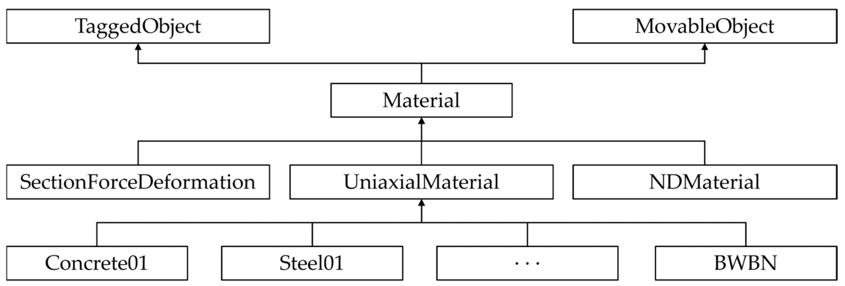
OpenSees organizes constitutive laws through a modular material library. In the material library, uniaxial cyclic behavior is represented through the abstract class UniaxialMaterial, while section-level force–deformation relationships and multiaxial constitutive responses are handled by SectionForceDeformation and NDMaterial, respectively. In this work, we implement the BWBN model as a uniaxial material to target uniaxial cyclic calibration data. Constitutive coupling under multi-directional loading is outside the scope of this paper.
To enable direct use of the complete twelve-parameter BWBN formulation described in
Section 2, we implemented a full BWBN uniaxial material within the OpenSees
UniaxialMaterial module. In OpenSees, the base Material class inherits from both
TaggedObject and
MovableObject, where the former provides a unique integer tag for identifying each material instance and the latter supports object communication and state transfer. The resulting class hierarchy for the BWBN material in OpenSees is illustrated in
Figure 2.
For each trial deformation increment, the material updates the BWBN internal state by integrating the evolution equation of the hysteretic variable and tracking the accumulated hysteretic demand required by the degradation and pinching terms. A local iterative update is used for this state integration, controlled by a user-specified tolerance and a maximum number of iterations. The updated state is then used to assemble the restoring stress and a consistent tangent stiffness, ensuring compatibility with the global equilibrium iterations.
For practical use, the full BWBN material is exposed through a dedicated Tcl command, as shown in Listing 1. In this work, the command accepts the twelve BWBN parameters, the initial stiffness, and the numerical controls for the local iterative update:
| Listing 1. Tcl command for the proposed BWBN material in OpenSees. |
| uniaxialMaterial BWBN $matTag $alpha $beta $gamma $n $deltaEta $deltaNu $zetas $q $p $Psi $deltaPsi $lambda $ko $tolerance $maxNumIter |
Here, $alpha, $beta, $gamma, and $n control the basic hysteresis shape, $deltaEta and $deltaNu govern stiffness and strength degradation, and $zetas, $q, $p, $Psi, $deltaPsi, and $lambda define the pinching behavior. The parameter $ko denotes the initial stiffness, while $tolerance and $maxNumIter control the convergence of the local state update within each global analysis step.
With this implementation, the complete twelve-parameter BWBN representation identified from cyclic test data can be assigned directly to OpenSees structural components and used immediately in nonlinear simulations, overcoming the limitations of the existing incomplete BWBN-related material and supporting a wider range of degrading and pinched response scenarios. Because the 12 BWBN parameters are highly coupled and costly to calibrate with conventional methods, we next present a physics-constrained, model-based inverse analysis for efficient parameter identification.
4. Physics-Constrained Inverse Identification of BWBN Parameters
4.1. Physics-Constrained Inverse Identification Formulation
4.1.1. Problem Statement
This section first describes the inverse identification formulation and the associated numerical workflow, and then reports validation results based on cyclic RC column tests. Using the notation established in
Section 2 and
Section 3, the identification of the BWBN model is formulated as a physics-constrained inverse problem driven by a measured cyclic force–displacement record. The inputs are the experimental dataset, consisting of a prescribed displacement history and the corresponding measured restoring force at discrete sampling points. The output is a single set of BWBN parameters that reproduces the observed hysteretic response when inserted into the same discrete constitutive update scheme used for forward simulation and thus can be directly implemented in numerical platforms such as OpenSees.
In this work, only the 12 BWBN parameters are treated as decision variables:
All other quantities required for computing the forward response follow the definitions and conventions already introduced in
Section 2 and
Section 3, and are kept fixed during the identification unless explicitly stated otherwise. A key feature of the proposed framework is that the “physics” is not imposed via an additional differential-equation residual penalty. Instead, the internal hysteretic state (e.g., the BWBN internal variable and the degradation-driving measure) is computed by incrementally integrating the BWBN evolution law along the prescribed displacement history. For each candidate
θ, the response is obtained by incrementally enforcing the BWBN state evolution via local updates, thereby constraining the inverse search to physically admissible trajectories.
To clarify the methodological positioning, prior BWBN identification studies can be broadly grouped into metaheuristic calibrations (e.g., differential evolution and particle swarm optimization), regression-based parameter predictors, and PINN-style approaches that enforce the evolution through residual penalties. These methods can fit cyclic loops well, but the calibration procedure does not always follow the same incrementally consistent state update used in nonlinear analysis platforms. Here, the BWBN evolution is enforced through an implicit incremental constitutive update at every recorded step, so the search is restricted to incrementally admissible trajectories and the identified parameters can be used directly in the full twelve-parameter OpenSees material. The advance is therefore incremental physical consistency and engineering deployment, rather than a new optimizer. The parameter identification is then posed as a bound-constrained nonlinear least-squares problem:
where
fiexp and
fimod(
θ) denote the experimental and model-predicted restoring forces,
fsc is a scaling constant for numerical conditioning, and
ρ(·) is the loss function. The feasible set Ω enforces physically admissible parameter bounds, taken from the reference ranges summarized in
Table 1.
4.1.2. Discrete Forward Model: Incremental BWBN State Evolution
For any candidate parameter set
θ, the model-predicted force history is obtained by incrementally integrating the BWBN evolution law along the prescribed displacement record. At each sampling point, the internal hysteretic variable
μz is updated through a local state-update procedure, while the degradation-driving measure
εn is accumulated to control deterioration and pinching. The restoring force is then evaluated using the force–state relation defined in
Section 2 and
Section 3.
The BWBN internal variable is advanced by an implicit incremental update. For
i ≥ 1,
where Δ
μi =
μi −
μi−1,
= Δ
μi/Δ
t, Δ
t denotes the sampling time step. Because
μz,i appears on both sides of Equation (14), the state update is solved locally at each increment using a fixed-point iteration, starting from
μz,i(0) =
μz,i−1 and iterating until the change in
μz is below a prescribed tolerance (or a maximum number of iterations is reached). This local update enforces the constitutive evolution directly during the forward computation.
Pinching is introduced through the smooth modifier
h(
μz,
εn) defined in Equation (8). In the discrete forward solver,
h(·) is evaluated at each increment using
μz and
εn in a lagged manner consistent with Equation (14), so that pinching evolves with cyclic loading. The accumulated measure
εn is updated incrementally using a trapezoidal quadrature of the hysteretic work:
Here ∆
μi =
μi −
μi−1 is the signed displacement increment over the full cyclic history (loading, unloading, and reloading). In the implementation, Equation (15) is evaluated incrementally using trapezoidal quadrature, where the trapezoidal average reduces one-sided numerical bias in the work accumulation and improves reproducibility. With
μz,i and
εn,i obtained from Equations (14) and (15), the restoring force sequence is computed using the force–state relation in
Section 2 and
Section 3, thereby completing the discrete forward operator required by the inverse identification in Equation (13).
4.1.3. Loss Definition and Constraint Enforcement
With the discrete forward operator defined above, the inverse identification reduces to minimizing the mismatch between the experimental and model-predicted restoring forces over the full cyclic record. The residual vector is constructed pointwise from the difference fimod(θ) − fiexp, and is scaled by a constant fsc for numerical conditioning (e.g., the peak absolute experimental force). This scaling improves the robustness of the optimization with respect to changes in force magnitude across different specimens and loading protocols.
The loss function ρ(·) in Equation (13) can be selected as the standard quadratic loss to recover a classical least-squares calibration. To mitigate the influence of sporadic measurement noise or a small number of outliers in the cyclic record, a robust loss (such as a smooth L1-type penalty) may alternatively be employed. Importantly, the use of robust losses does not alter the physics constraint, because the BWBN evolution is enforced through the discrete solver at each increment; it only changes how the data misfit is aggregated during the parameter update.
Physically admissible bounds are enforced as hard constraints throughout the optimization, using the reference ranges summarized in
Table 1. These bounds incorporate prior knowledge and prevent unstable parameter combinations during the implicit state update in Equation (14). Consequently, the identified parameters are both data-consistent and directly transferable to subsequent simulations.
4.2. Numerical Implementation and Optimization Workflow
The physics-constrained identification is implemented as a bound-constrained nonlinear least-squares problem driven by the experimental cyclic record. Force residuals are scaled by
fsc for numerical conditioning and the time step Δ
t is taken as the sampling interval. For each trial parameter vector
θ, the objective evaluation requires a single forward pass through the record. Hence, one objective evaluation corresponds to one complete forward sweep over the record, and the implementation-controlled convergence statistics are summarized later. The internal variable
μz,i is obtained at each increment by the implicit update in Equation (14), solved locally via a fixed-point iteration. Pinching is evaluated using
h(·) from Equation (8), and the degradation-driving measure
εn is updated by the trapezoidal rule in Equation (15). The restoring force sequence is then computed using the force–state relation defined in
Section 2 and
Section 3.
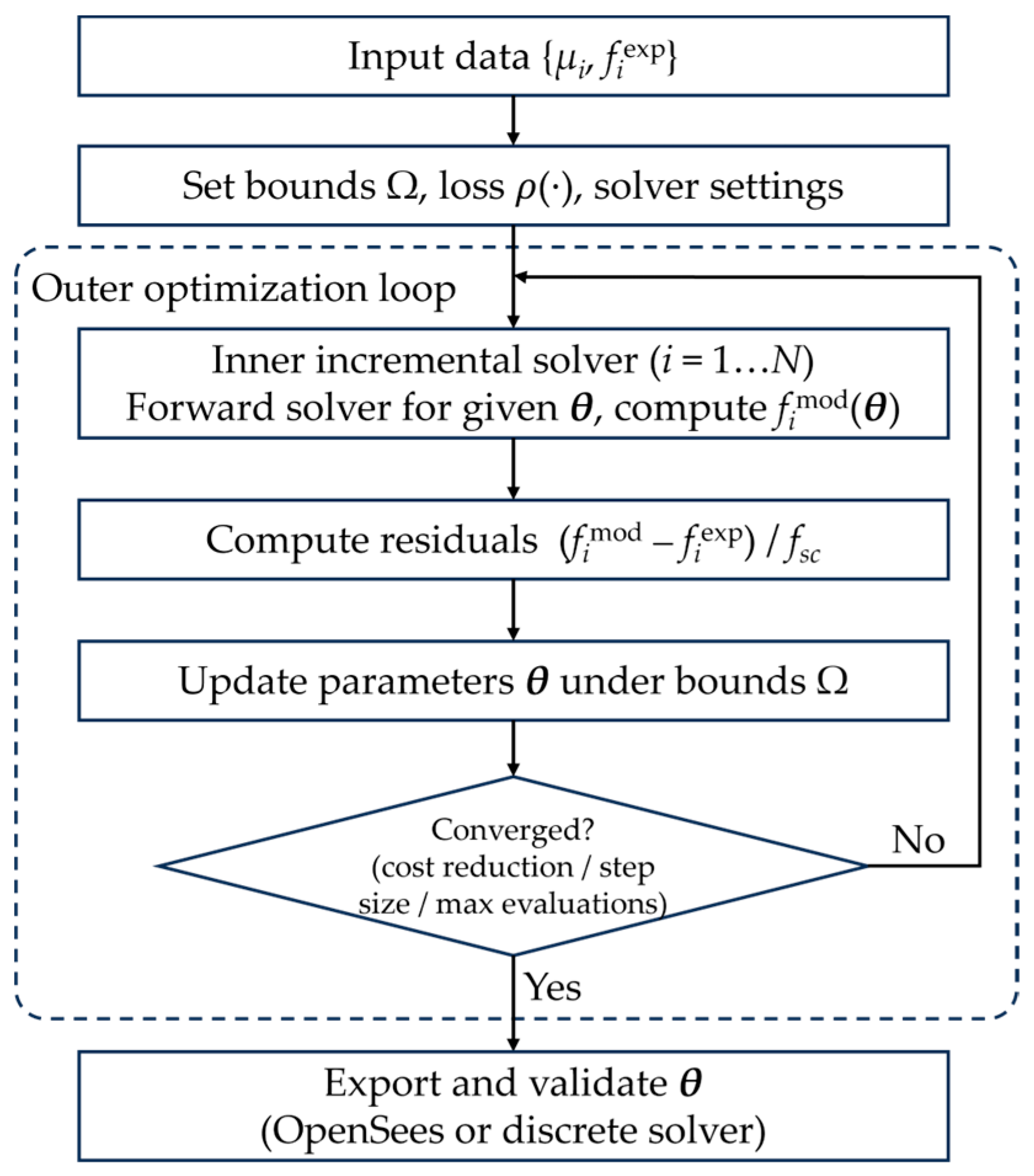
Parameter updates are performed under hard bounds Ω using a trust-region reflective least-squares solver, which terminates when the reduction in the objective function or the parameter step becomes sufficiently small, or when the maximum number of function evaluations is reached. The complete numerical workflow, highlighting the outer optimization loop and the inner incremental solver, is summarized in
Figure 3. The identified parameter sets are then exported for forward re-simulation and evaluated against the experimental hysteresis responses, as reported in
Section 4.3.
In the present implementation, the 12-parameter identification is solved by a bound-constrained trust-region reflective nonlinear least-squares algorithm with a robust loss function. The total number of residual evaluations is explicitly capped (Nfev ≤ 400); each evaluation performs one full displacement-driven BWBN forward sweep over the cyclic record, advancing all internal variables incrementally at every step. Accordingly, the number of forward constitutive integrations per specimen is bounded by Nfev, and the cost of a single forward sweep scales as O(N·I), where N is the number of data points and I is the fixed-point iteration count per increment (tolerance 10−3, maximum 2000 iterations). This design is deterministic and reproducible, provides explicit control of computational effort through bounds and Nfev, and improves robustness via residual scaling and the robust loss. Moreover, since the same incrementally consistent update is used in the OpenSees material implementation, the identified parameters are directly deployable for nonlinear structural simulations.
Representative profiling of the current CPU-based Python 3.11.9 implementation shows that the local fixed-point constitutive update is relatively inexpensive compared with the outer nonlinear least-squares loop. All profiling results reported here were obtained on a personal computer equipped with an Intel(R) Core(TM) Ultra 7 155H processor (1.40 GHz), 32 GB RAM, and a 64-bit Windows operating system. For a record with about 600 points, the identification converged in 65 function evaluations with a wall-clock runtime of about 7 s; the average fixed-point iteration count was about 2.27 per displacement step, with a maximum of 3. For a longer record with about 1500 points, the profiling run reached 71 function evaluations in about 19 s, while the average fixed-point iteration count remained about 2.26 and the maximum was 4. For a substantially longer record with about 11,000 points, the profiling run reached 102 function evaluations with a wall-clock runtime of about 182 s, while the average fixed-point iteration count remained about 2.26 per displacement step and the maximum was 4. These representative results confirm that the dominant computational cost lies in the repeated full-record forward sweeps within the nonlinear least-squares procedure, whereas the local constitutive update itself remains relatively cheap.
4.3. Validation on RC Column Tests with Different Failure Modes
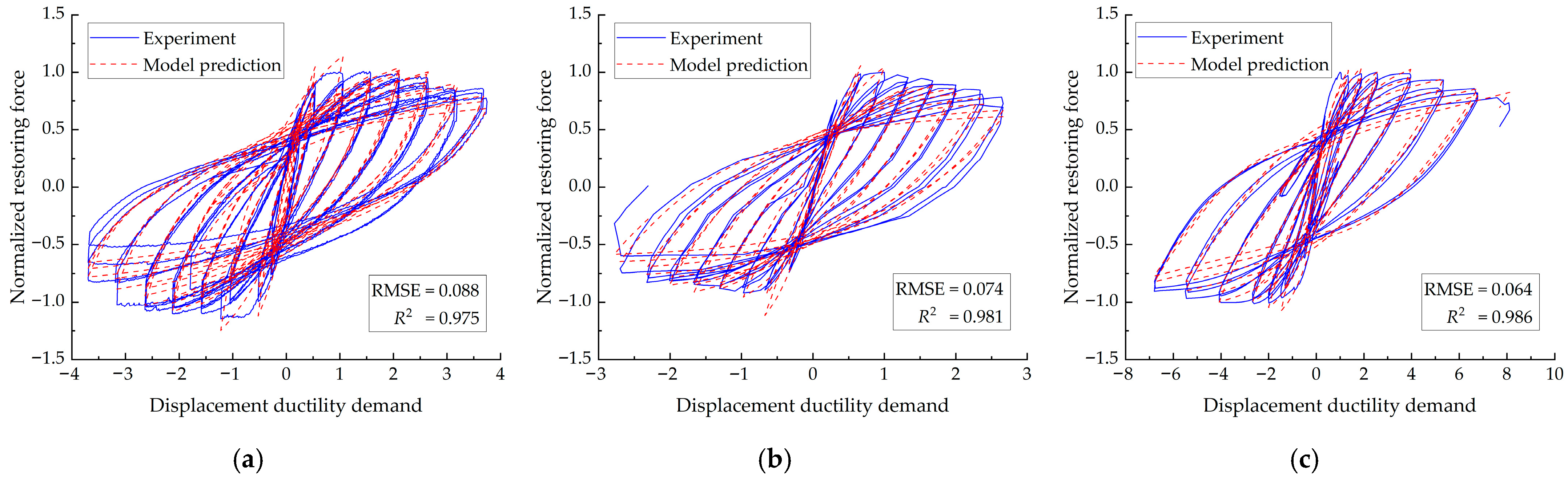
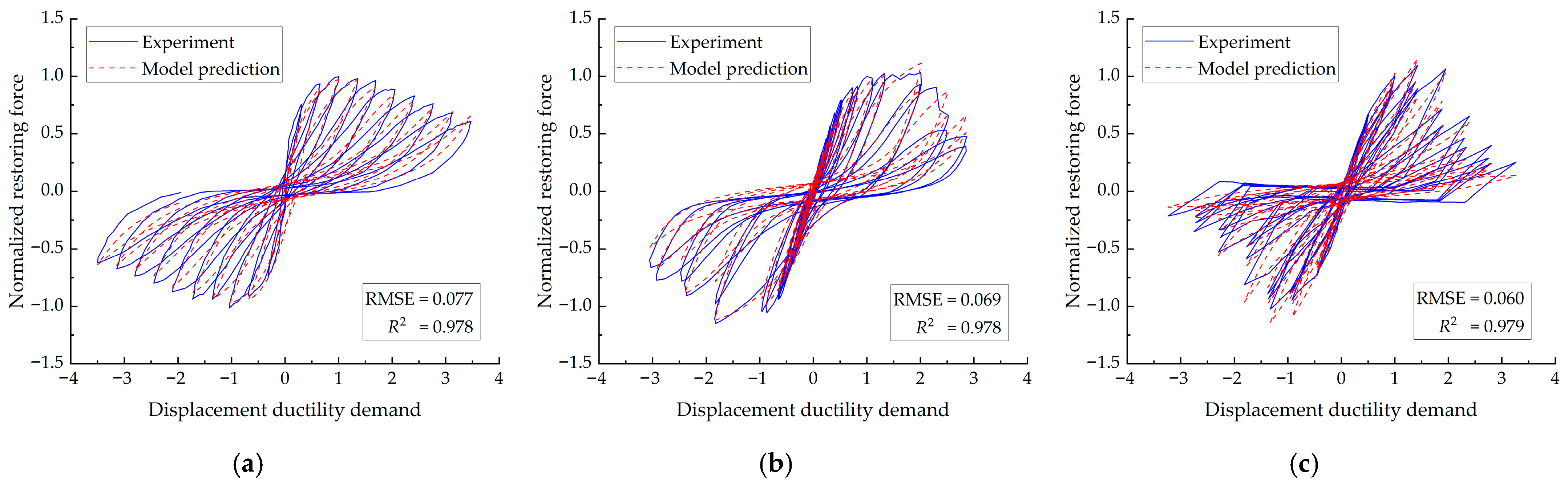
The proposed identification procedure is validated using nine RC column tests covering three representative failure modes: flexural failure (FF), flexural–shear failure (FS), and shear failure (SF). The selected specimens and their key design and demand descriptors are summarized in
Table 2, including the span-to-depth ratio, axial load ratio, and longitudinal and transverse reinforcement ratios. For each specimen, the loading protocol, clamping conditions, axial load application, and key material properties are reported in the corresponding source publication listed in
Table 2. In this study, we use the reported cyclic force–displacement records under the prescribed axial load ratio, while the original reports provide the full test setup details needed to interpret the results.
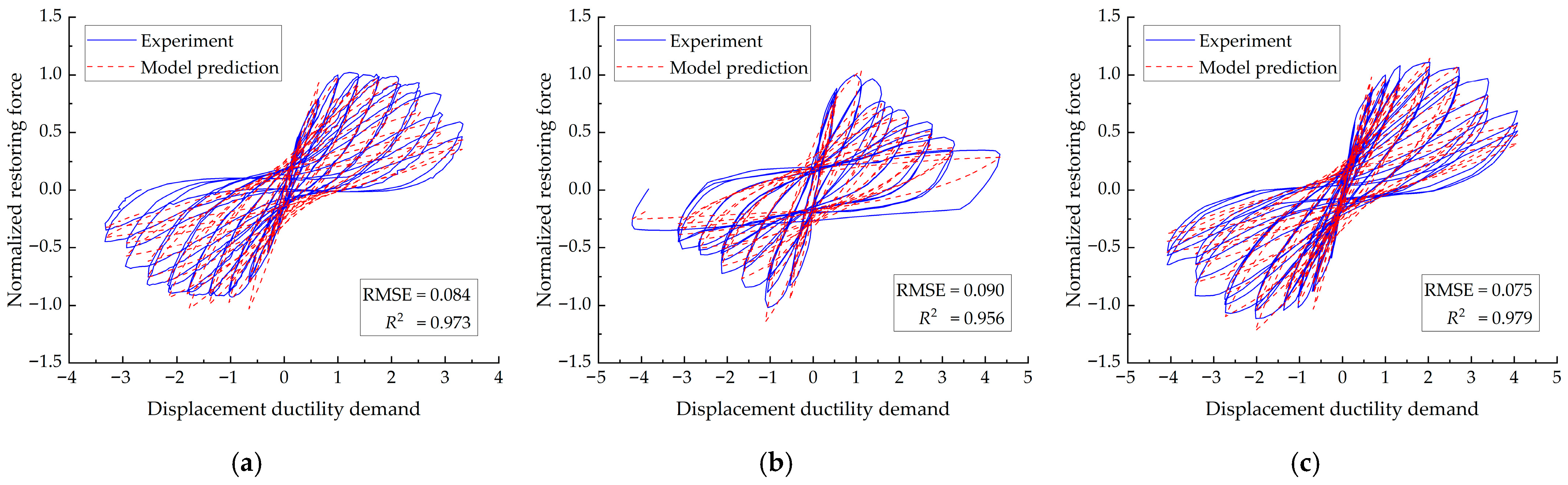
For each specimen, the proposed identification procedure is applied to calibrate the BWBN parameter vector from the measured cyclic force–displacement record. Model performance is assessed by overlaying the simulated and experimental hysteresis loops and by reporting the root mean square error (RMSE) and the coefficient of determination
R2 over the full record. The results are presented by failure mode, with FF, FS, and SF specimens shown in
Figure 4,
Figure 5 and
Figure 6, respectively, to facilitate a direct comparison of accuracy and mode-dependent response characteristics.
Overall, the calibrated BWBN model provides good agreement with the measured hysteresis loops across the three failure modes, as reflected by the loop overlays and the reported RMSE and R2. In addition to RMSE and R2, the maximum absolute deviation normalized by the peak experimental force, MaxAE(%), is reported to quantify the worst-case pointwise mismatch. The MaxAE(%) values are 19.0%, 22.7%, and 18.7% for S1–3; 21.5%, 27.1%, and 21.1% for S4–6; and 25.2%, 20.9%, and 15.8% for S7–9, respectively. MaxAE(%) is a conservative pointwise metric defined by the single largest deviation over the entire cyclic record. It is therefore more sensitive than RMSE and R2 to localized segments with sharp reversals, pinching, or rapid deterioration, and is reported here as a complementary indicator. The following section discusses the mode dependent characteristics, typical sources of mismatch, and the implications and limitations of the identified parameter sets.
5. Discussion
This section interprets the identification results from the perspective of failure mode-dependent degradation and pinching behavior. We discuss where the remaining discrepancies concentrate in the cyclic record and why these segments are more challenging to capture, and we summarize the implications for parameter identifiability.
Figure 4,
Figure 5 and
Figure 6 show that the identified BWBN model reproduces the main hysteretic features of the nine tests across the three failure modes. The model captures the backbone strength, the cycle-dependent reduction in secant stiffness, the unloading stiffness, and the degree of reloading pinching. The RMSE and
R2, annotated in each panel, provide a global quantitative summary over the full cyclic record and corroborate the observed agreement.
For the FF specimens (
Figure 4), the response is dominated by flexural yielding and typically exhibits relatively stable energy dissipation with gradual degradation. In these cases, the identified model matches the overall loop width and the post-yield hardening and softening trend well. The remaining mismatches are most often localized around displacement reversals and early reloading segments. These portions of the record are sensitive to the smoothness of the transition from unloading to reloading and to the relative contribution of elastic versus hysteretic components, such that small differences in the identified transition parameters may lead to visible deviations even when the global metrics remain favorable.
For the FS specimens (
Figure 5), the hysteresis loops reflect the interaction between flexural yielding and shear-related deterioration, leading to more pronounced cycle-by-cycle stiffness loss and strength decay at larger deformation demands. The identified model generally tracks the evolution of the envelope and the degradation trend. However, discrepancies may increase near peak excursions and during stiffness recovery after load reversals. This behavior is consistent with stronger coupling among degradation and pinching-related parameters under FS-type responses, where multiple mechanisms contribute simultaneously to the observed stiffness and strength reduction.
For the SF specimens (
Figure 6), the hysteresis response is generally more pinched with lower energy dissipation and may exhibit abrupt strength drops. The identified model reproduces the overall pinched morphology and the deterioration-induced strength reduction, whereas the largest deviations are typically observed along reloading branches and in cycles with sudden strength loss. Such localized features are challenging to fit with a smooth phenomenological evolution law and are often less well constrained by global force–displacement data, so different parameter combinations may yield similar overall errors while differing in specific reloading segments, implying reduced identifiability of some degradation and pinching parameters for shear-dominated behavior.
To make the above interpretation more quantitative, the calibrated degradation- and pinching-related parameters were further compared directly across the three failure-mode groups. For the FF specimens, δη remained at or near its lower bound in all three cases, while δν ranged from 0.025 to 0.1, consistent with relatively mild deterioration. For the FS specimens, the pinching-related parameters shifted toward larger p and ψ values (p = 2.08–4.99, mean 3.57; ψ = 0.70–2.22, mean 1.68) than in the FF group (p = 0.44–4.22, mean 2.31; ψ = 0.35–0.85, mean 0.58), indicating that the mixed flexural–shear responses required stronger reloading distortion to reproduce the measured loops. In the present dataset, the SF specimens were characterized by much smaller q and ψ values (q = 0.061–0.076, mean 0.070; ψ = 0.093–0.173, mean 0.122). This combination is consistent with the more pinched loops and more abrupt strength loss observed in the shear-dominated tests. Not all parameters vary monotonically with failure mode, which suggests that the distinctions among FF, FS, and SF responses are encoded by combinations of BWBN parameters rather than by any single coefficient.
Across the calibrated results, the parameter magnitudes show consistent shifts with failure mode. For the flexure-dominated specimens, the identified deterioration effects are generally mild, reflected by relatively smaller degradation parameters δν and δη, and the pinching severity is limited, corresponding to smaller values of the key pinching-intensity parameters (e.g., ζs and λ). For the flexural–shear specimens, both degradation and pinching become more pronounced, and the identified solutions typically move toward larger δν–δη and stronger pinching settings, consistent with the increased cycle-by-cycle stiffness loss and strength decay at larger excursions. For the shear-dominated specimens, the more constricted loops and occasional abrupt strength drops are generally associated with the largest degradation effects (larger δν, δη) and the strongest pinching intensity (higher ζs, λ), together with pinching-evolution terms that promote faster development of reloading constriction as energy accumulates. Because these parameters are identified in a coupled manner, the above trends are most meaningful at the level of the degradation and pinching parameter groups, which provides a mechanistic interpretation of how failure mode influences the calibrated BWBN behavior.
To quantify which BWBN parameters are most informed by the cyclic record, we performed a local sensitivity check at the identified solution using the Jacobian returned by the least-squares solver. After normalizing parameters by their bound ranges, sensitivity indices were computed from the column norms of the Jacobian and used to rank parameter influence near the optimum. The results indicate that the calibration is dominated by the hysteretic-shape parameters β and γ, whereas p, λ, and n are among the least sensitive parameters and are therefore less constrained by the global force–displacement record. It should be noted that this Jacobian-based sensitivity ranking is a local indicator evaluated at the identified solution and does not by itself establish the global identifiability or strict uniqueness of the full twelve-parameter BWBN vector. Because degradation and pinching-related parameters are strongly coupled, different parameter combinations within the admissible bounds may still produce similar global hysteretic errors, especially for shear-dominated cases. Therefore, the calibrated results in the present study are interpreted primarily at the level of physically meaningful parameter groups, rather than as evidence that every individual parameter is uniquely determined from a single cyclic record. A more formal assessment of parameter correlation, multi-start stability, and global identifiability will be considered in future work.
In addition to the local sensitivity ranking, the residual Jacobian at the converged least-squares solution was used to obtain a first-order local uncertainty estimate for the identified parameters. For the representative FS specimen analyzed here, the fit remains good, while the uncertainty levels differ markedly across parameter groups. The dominant shape parameters β and γ show normalized sensitivities of 1.000 and 0.9995, with range-normalized standard deviations of 0.1197 and 0.1012, respectively, indicating that the main hysteretic-shape parameters are relatively well constrained by the cyclic record. By contrast, the pinching-related group has the largest mean range-normalized uncertainty (0.3276), compared with 0.1528 for the degradation group and 0.1015 for the shape group, suggesting that pinching-related parameters remain the least constrained in the present specimen. These results are broadly consistent with the expected strong coupling of BWBN pinching parameters, although parameter influence on the fit does not necessarily imply equally strong identifiability for every individual coefficient. The estimate is local in nature and does not by itself establish global uniqueness of the calibrated BWBN parameter set.
To examine whether the identified parameters retain predictive capability beyond the fitted segment of the cyclic record, a simple prefix hold-out validation was conducted. Specifically, the BWBN parameters were identified using only the first two-thirds of the measured force–displacement history (identification segment), and the obtained parameters were then kept fixed, without any re-calibration, to generate the response over the remaining one-third of the record (prediction segment). This within-record check directly evaluates generalization under progressively stronger degradation and pinching. The prefix hold-out results for all nine specimens are summarized in
Table 3 in terms of
R2 and RMSE for both the identification and prediction segments. For the held-out prediction segments, the results indicate that the calibrated parameter sets generally retain useful predictive capability for the unseen portion of the cyclic record. The remaining discrepancies are mainly localized around displacement reversals and early reloading segments, where pinching transitions and deterioration evolution are most sensitive to coupled parameters, and are generally more noticeable in cases with more abrupt deterioration or stronger shear-dominated behavior.
Overall, the fit is strongest for flexure-dominated tests and degrades for shear-dominated cases with stronger pinching and more abrupt deterioration. Because the forward evaluation enforces the discrete BWBN evolution at every increment, the identified parameter sets remain physically consistent and can be used directly in OpenSees for further simulations. The calibrated BWBN parameters therefore support consistent hysteresis reproduction and straightforward deployment in structural analysis platforms for response prediction and comparative studies.
Although the validation cases cover multiple RC column failure modes and demonstrate that the proposed framework can reproduce representative degrading and pinched hysteresis behaviors, the current dataset remains limited in size relative to the twelve-dimensional BWBN parameter space. Therefore, the present results should be interpreted as a representative validation of feasibility and engineering applicability, rather than as a statistically comprehensive basis for establishing broadly generalizable parameter trends. A larger-scale evaluation using broader experimental databases of RC columns and related structural components will be needed in future work to more rigorously assess robustness, generalizability, and cross-dataset consistency of the identified parameter sets.
6. Conclusions
This study addresses the gap between high-dimensional BWBN calibration and reproducible engineering deployment by developing a physics-constrained, model-based inverse identification framework for degrading and pinched hysteresis. The scientific focus is on achieving numerically stable and incrementally consistent parameter identification for a strongly coupled internal-variable model, while producing parameter sets that can be transferred directly to a simulation platform.
A complete twelve-parameter BWBN uniaxial material is implemented in OpenSees to represent energy-dependent degradation and pinching. The identification is posed as a bound-constrained nonlinear least-squares problem, and each objective evaluation is carried out by a discrete incremental constitutive update that advances the BWBN internal state and updates the energy-driven deterioration step by step. This discrete forward operator enforces state-evolution consistency during inversion and supports the direct use of the identified parameters in nonlinear structural simulations.
Validation on nine RC column tests covering flexural, flexural–shear, and shear failures shows that the identified model reproduces the main hysteretic characteristics across failure modes. The agreement is strongest for flexure-dominated responses, while accuracy decreases for shear-dominated cases where pinching and abrupt deterioration are more pronounced, highlighting the practical challenges associated with strongly coupled degradation parameters.
Future work will focus on extending the framework to biaxial loading, expanding validation to additional datasets and loading protocols, and broader uncertainty quantification, particularly for shear-dominated behavior.