A Simplified Model of a Solar Water Heating System with Phase Change Materials in the Storage Tank

Abstract

The intermittent and variable nature of solar energy poses challenges for maintaining stable thermal performance in solar heating systems. One effective approach to mitigate this limitation is to store surplus thermal energy during periods of high solar irradiance and release it when solar input is insufficient. Phase change materials (PCMs) are particularly suitable for this purpose due to their ability to absorb and release large amounts of latent heat during phase transition. The aim of this work is to develop a mathematical model of a flow-through tank containing a phase change material in the form of a spherical packed bed. Including longitudinal dispersion in the model equations allows for a more accurate description of the heat transfer process in a tank containing PCM elements. Simulation calculations based on the model were carried out to demonstrate its potential applicability to practical problems. The influence of the following parameters on the process was investigated: tank volume, water flow rate, phase change temperature, process duration, dispersion coefficient during water flow, radius of the packed-bed elements, and cyclic variations of the inlet water temperature. A significant influence of the axial dispersion coefficient in the tank containing PCM on the outlet water temperature profile was demonstrated. It was found that the internal heat transfer coefficient within the packing elements containing PCM falls within the range of 58–145 W/(m²K).

1. Introduction

Thermal energy storage (TES) plays a central role in improving the efficiency and reliability of energy systems based on renewable energy sources. By decoupling energy production from demand, TES mitigates the intermittency of solar energy and enables more flexible operation of heating and domestic hot water systems. Among available TES technologies, systems combining sensible and latent heat storage offer an attractive compromise between energy density, operating temperature stability, and system complexity.

Phase changes and the associated release and absorption of heat play an important role in natural systems. Melting and freezing of water are key processes regulating atmospheric temperature due to the high latent heat of phase transitions. Freezing (solidification) releases heat to the surroundings, mitigating temperature drops during winter, whereas melting of ice and snow absorbs heat, limiting rapid warming in spring. These processes influence ocean currents, atmospheric circulation, extreme weather phenomena, and sea level.

Energy storage can be achieved by utilizing latent heat generated during the phase change of the storage material (PCM). The most commonly used PCMs include paraffins, fatty acids and esters, and salt hydrates. Recent advances in PCM research involve incorporating nanoparticles—such as aluminum oxide, tin oxide, iron oxide, gold, titanium dioxide, copper oxide, carbon nanotubes, diamond, and silver—to enhance their thermophysical properties, primarily by increasing thermal conductivity, reducing supercooling effects, and improving heat transfer rates during melting and solidification.

When integrated into water-based storage systems, PCMs can increase effective storage capacity without a proportional increase in tank volume, while simultaneously stabilizing the outlet temperature during charging and discharging.

PCM-based TES systems have been investigated in various applications, including solar heating and cooling systems, thermal comfort enhancement in buildings and vehicles, as well as thermal protection of food, electronics, and medical products. PCMs have been widely investigated for photovoltaic applications as a means of limiting operating temperature and improving electrical efficiency [1,2,3].

In the building sector, PCMs have been integrated into envelope components to moderate indoor temperature fluctuations and reduce heating and cooling loads. Numerous studies have focused on PCM-enhanced wall systems, including Trombe walls, demonstrating their potential to improve indoor thermal comfort and reduce energy demand [4,5,6]. Beyond walls, PCM integration has also been explored for floors [7,8] and roofs [9,10,11], highlighting the versatility of PCMs as passive or hybrid thermal storage elements.

In parallel with building-scale applications, increasing attention has been devoted to the integration of PCMs into water storage tanks, particularly for solar water heating and domestic hot water systems. The primary engineering objective in these systems is to increase the usable thermal capacity and extend the duration of stable outlet temperature.

Early experimental work by Cabeza et al. [12] demonstrated that even a small amount of PCM can significantly affect tank performance. In a solar heating system with a 146 L storage tank, the addition of 3 kg of a PCM–graphite compound was sufficient to compensate heat losses of 3–4 °C in the upper tank region over approximately 10 h. Similar conclusions were reported by Mehling et al. [13]. In the study by Bianqui et al. [14], temperature measurements were carried out in cylindrical stainless-steel capsules containing paraffin as the PCM.

A frequently used PCM is sodium acetate trihydrate (SAT), a salt hydrate, often applied as a sodium acetate trihydrate-based composite with a liquid polymer and additional water. SAT exhibits a latent heat of fusion of 264 kJ/kg and a melting temperature of 58 °C. These thermal properties make SAT a suitable material for integration with solar heating systems, space heating, and domestic hot water preparation [15,16].

Several studies have combined experimental investigations with system-level modeling to quantify the practical benefits of PCM-enhanced tanks. In the study by Wang et al. [17], thermal energy storage was investigated in a tank containing 137.8 kg of PCM and 75 L of water. Sodium acetate trihydrate was used as the PCM. The thermal performance and flow characteristics of the heat storage system were analyzed using both experimental measurements and CFD simulations. Koželj et al. [18] showed experimentally that incorporating approximately 15% PCM into a water storage tank increased stored thermal energy by about 70% compared with a conventional tank. Pop and Balan [19] demonstrated numerically that PCM integration in domestic hot water tanks can reduce the required storage volume by 25% and lower fuel consumption and CO₂ emissions by 5–12% in high-demand applications. Najafian et al. [20] used TRNSYS simulations combined with artificial neural networks and genetic algorithms to optimize PCM content and container geometry, showing that properly designed PCM tanks can shift electricity consumption entirely to off-peak periods while maintaining hot water availability. In the work of Bouhal et al. [21], the operating cycle of solar thermal energy storage systems was simulated. Two different models accounting for phase change heat were analyzed. Longitudinal heat transport by conduction was included in the process model. In the mathematical model presented by Kong et al. [22], heat transfer coefficients between water and PCM were determined separately for the charging and discharging periods. The process model accounted for axial heat conduction in the tank as well as heat losses to the surroundings. The studies were conducted in a tank with a diameter of 0.4 m and a height of 1.7 m, containing 112 steel tubes with a diameter of 27.6 mm filled with PCM.

Detailed CFD models have been employed to analyze melting and solidification dynamics and heat transfer enhancement mechanisms, such as the dynamic melting concept proposed by Tay et al. [23].

The aim of this work is to develop a mathematical model of a flow-through tank containing a phase change material in the form of a spherical packed bed. Melting and solidification of the PCM occur inside spherical elements of the bed. The process is transient in nature, while the PCM bed itself is stationary. Assuming that radial variations in the tank can be neglected, three independent variables are considered: the axial coordinate along the tank height z, the radial coordinate within a spherical packing element r, and time t. One of the simplifying assumptions of the model is the elimination of the spatial coordinate inside the sphere. Calculations based on the proposed model do not require complex numerical procedures; the only numerical operation involved is the solution of a system of linear algebraic equations.

In the model, water flow through the tank is assumed to be dispersive. The longitudinal dispersion coefficient accounts for axial mixing phenomena in the flow apparatus. These include mixing caused by convective currents and turbulent eddies, as well as mixing resulting from velocity non-uniformities during fluid flow. Dispersion leads to a reduction in the driving force for heat (or mass) transfer between the phases involved in the process. A reduced driving force (temperature difference) results in a lower intensity of heat transfer. In the model, longitudinal dispersion is treated as a process analogous to diffusion; therefore, dispersion is described using a Fick/Fourier-type equation in which the diffusion coefficient is replaced by the dispersion coefficient. Unlike molecular diffusion coefficients (mass or thermal), the dispersion coefficient is not a molecular property and must be determined experimentally or from empirical correlations appropriate for the given process conditions. Introducing dispersion into the model equations required the application of an appropriate inlet boundary condition [24,25].

A simplified relation describing the rate of heat transfer between the surface of a spherical packing element and its interior was incorporated into the model equations. This relation, known as the Linear Driving Force (LDF) formulation and described in Appendix A.1 [26,27,28], links the heat transfer rate to the driving force of the process, defined as the difference between the sphere surface temperature and the average temperature inside the sphere. The proportionality coefficient in this relation, i.e., the heat transfer coefficient h, can be determined in simple cases. However, due to the complexity of the processes occurring during PCM melting and solidification, as well as the presence of supercooling effects, the heat transfer coefficient in the proposed model should be treated as a parameter to be determined empirically.

Simulation calculations based on the model were carried out to demonstrate its potential applicability to practical problems. The influence of the following parameters on the process was investigated: tank volume, water flow rate, phase change temperature, process duration, dispersion coefficient during water flow, radius of the packed-bed elements, and cyclic variations of the inlet water temperature.

2. Process Model

2.1. Assumptions

The presented model is based on the following assumptions:

• The tank is filled with spherical elements containing PCM.
• Water flows through the tank with packed bed. The flow is dispersive in nature. Axial mixing can be described by an equation analogous to Fick’s law, and the intensity of mixing is characterized by the dispersion coefficient.
• During heat transfer between the water phase and the PCM contained in the capsules, the dominant thermal resistance is located inside the capsule.
• Heat transfer within a spherical element containing PCM can be described using a Linear Driving Force (LDF) formulation.

2.2. Enthalpy of Phase Change Materials

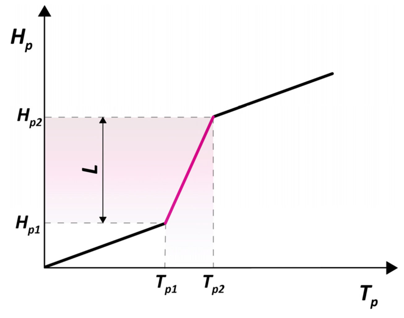
When modeling processes involving phase change materials, it is convenient to use enthalpy-based formulations. Assuming that the phase change occurs over the temperature range from T_p1 to T_p2, the enthalpy of the material at temperature T_p can be calculated using relation (1), where c_s and c_L denote the specific heats of the solid and liquid phases, respectively, and L is the latent heat of phase change [22,29]:

$$H_p=\{\begin{array}{c}{c}_s{T}_p \mathrm{for} { T}_p<T_{p1}\\ H_{p1}+{\displaystyle \frac{T_p-T_{p1}}{T_{p2}-T_{p1}}}·L \mathrm{for} T_{p1}<T_p<T_{p2}\\ H_{p2}+c_L\left(T_p-T_{p2}\right) \mathrm{for} T_p>T_{p2}\end{array}$$

(1)

Relation (1) can be generalized to the following form:

$$H_p=c_{PCM}{T}_p+b$$

(1a)

in which the constants c_PCM and b are defined as follows:

$${ c}_{PCM}=c_s \mathrm{a}\mathrm{n}\mathrm{d} b=0{ \mathrm{f}\mathrm{o}\mathrm{r} H}_p<H_{p1}$$

(1b)

$$c_{PCM}={\displaystyle \frac{L}{T_{p2}-T_{p1}}} \mathrm{a}\mathrm{n}\mathrm{d} b=H_{p1}-{\displaystyle \frac{L{T}_{p1}}{T_{p2}-T_{p1}}} { \mathrm{f}\mathrm{o}\mathrm{r} H}_{p1}<H_p<H_{p2}$$

(1c)

$$c_{PCM}=c_L \mathrm{a}\mathrm{n}\mathrm{d} b=H_{p2}-c_L{T}_{p2}{ \mathrm{f}\mathrm{o}\mathrm{r} H}_p>H_{p2}$$

(1d)

where the enthalpies H_p1 and H_p2 denote, respectively:

$$H_{p1}=c_S{T}_{p1}$$

(2)

$$H_{p2}=c_S{T}_{p1}+L$$

(3)

An interpretation of the above relations is shown in Figure 1.

Differentiating relation (1a) yields:

$${\displaystyle \frac{d{H}_p}{d{T}_p}}=c_{PCM}$$

(4)

2.3. Process Description

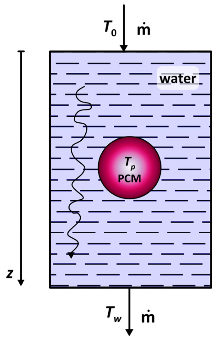
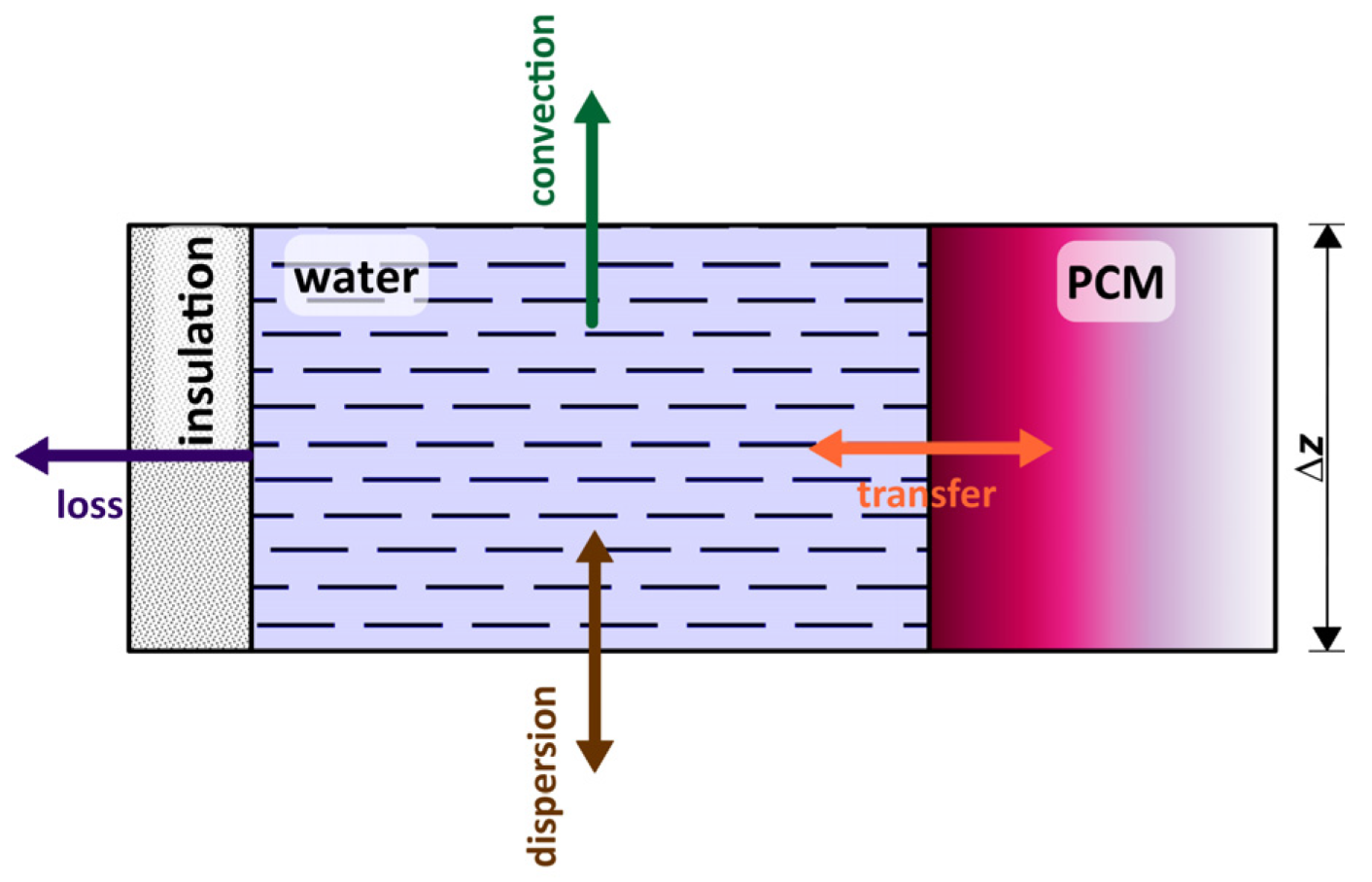
Figure 2 shows a schematic of water flow through a tank filled with a phase change material. The tank contains spherical elements. The PCM is enclosed in a shell impermeable to mass transfer.

Heat transfer occurs in the tank between the water and the PCM; the direction of this heat flux is variable and depends on the instantaneous relationship between the water and PCM temperatures. In Figure 2, the PCM is represented symbolically by a single sphere.

2.4. Heat Transfer Coefficient

The heat flux transferred between the water and the PCM contained in the capsules can be described by the heat transfer equation:

$${\displaystyle \frac{{\stackrel{·}{Q}}_p}{V_t}}=U_p{a}_b(T_w-T_p)$$

(5)

where U_p is the overall heat transfer coefficient and V_t is the bed volume. The reciprocal of U_p represents the total thermal resistance for heat transfer from the water to the interior of the packing elements. If the thermal resistance of the packing walls is negligible, then 1/U_p may be expressed as the sum of the external and internal resistances:

$${\displaystyle \frac{1}{U_p}}={\displaystyle \frac{1}{h_w}}+{\displaystyle \frac{1}{h}}$$

(6)

This results in a uniform wall temperature of the packing elements, T_wall, and leads to the following relationship:

$$U_p\left(T_w-T_p\right)=h\left(T_{wall}-T_p\right)$$

(7)

The quantity $a_b$ is the specific surface area of the bed, defined as the ratio of the contact surface area of the bed elements with the fluid to the bed volume. Heat transfer leads to changes in the PCM enthalpy, as described by the relation:

$${\stackrel{·}{Q}}_p=M_p{\displaystyle \frac{{dH}_p}{dt}}$$

(8)

where M_p is the mass of the PCM. Depending on the sign of the derivative, the direction of this heat flux may change. A positive value of the flux (and the derivative) indicates heat transfer toward the PCM elements, which corresponds to melting, provided that the PCM temperature lies within the melting range. Conversely, for a negative value of the derivative, solidification of the phase change material occurs within the temperature range between T_p1 and T_p2.

Based on relation (4), the time variation of the enthalpy can be expressed as:

$${\displaystyle \frac{d{H}_p}{dt}}=c_{PCM}{\displaystyle \frac{d{T}_p}{dt}}$$

(9)

Taking into account the relationship between the PCM mass and the bed volume:

$$M_p=V_t(1-\epsilon ){\rho }_p$$

(10)

from relations (8)–(10), it follows that:

$${\displaystyle \frac{{\stackrel{·}{Q}}_p}{V_t}}=(1-\epsilon ){\rho }_p{c}_{PCM}{\displaystyle \frac{d{T}_p}{dt}}$$

(11)

To determine the heat transfer coefficient, it was assumed that the spherical elements containing PCM consist of a homogeneous phase characterized by a thermal conductivity k_p. The problem is therefore reduced to transient heat conduction in a sphere with a first-kind (Dirichlet) boundary condition. In addition to the exact solution, simplified solutions exist for this case, the best known being the Linear Driving Force (LDF) formulation. Appendix A.1 derives an approximate expression for the heat transfer rate in a sphere. Expression (A5) was substituted into Equation (11), yielding:

$${\displaystyle \frac{{\stackrel{·}{Q}}_p}{V_t}}=15(1-\epsilon ){\displaystyle \frac{k_p}{R^2}}(T_{wall}-T_p)$$

(12)

The definition of the PCM thermal diffusivity was employed:

$$a_p={\displaystyle \frac{k_p}{{\rho }_p{c}_{PCM}}}$$

(13)

The specific surface area of the packing composed of spherical elements is given by:

$$a_b={\displaystyle \frac{3(1-\epsilon )}{R}}$$

(14)

Relation (14) was substituted into Equation (5), and the right-hand sides of Equations (5) and (12) were compared. Taking Equation (7) into consideration, the following expression for the heat transfer coefficient is obtained:

$$h=5{\displaystyle \frac{k_p}{R}}$$

(15)

2.5. Balance Equations

Figure 3 shows the heat fluxes involved in the process. The balance is formulated for a bed element of height $\mathsf{\partial }z$. The heat balance for the water phase is as follows:

$$D_E{\rho }_w{c}_w{\displaystyle \frac{{\mathsf{\partial }}^2{T}_w}{\mathsf{\partial }{z}^2}}-u{\rho }_w{c}_w{\displaystyle \frac{\mathsf{\partial }{T}_w}{\mathsf{\partial }z}}-U_p{a}_b(T_w-T_p)-{\displaystyle \frac{4U_t}{D}}(T_w-T_a)=\epsilon {\rho }_w{c}_w{\displaystyle \frac{\mathsf{\partial }{T}_w}{dt}}$$

(16)

The individual terms on the left-hand side of the equation represent, respectively, the heat fluxes due to dispersion, convection, interphase heat transfer, and heat loss to the surroundings. The dispersive term characterizes longitudinal mixing of water in the void spaces between the bed elements; in the absence of mixing, the parameter $D_E$ should be identified with the thermal diffusivity of water.

The convective term refers to water flow through the tank. A value of $u=0$ indicates the absence of water flow. Heat transfer between the water phase and the PCM is characterized by the heat flux per unit bed volume (Equation (5)).

Heat losses to the surroundings are described by the following expression:

$${\displaystyle \frac{{\stackrel{·}{Q}}_L}{V_t}}={\displaystyle \frac{4U_t}{D}}(T_w-T_a)$$

(17)

The term 4/D applies only to tanks of cylindrical geometry; it represents the ratio of the lateral surface area of the cylinder to its volume. The right-hand side of Equation (16) represents the accumulation term. A positive value of the derivative indicates heat accumulation in the water phase, corresponding to an increase in its temperature. A negative value of the derivative indicates cooling of the water, while a zero value implies no temperature change.

The heat balance for the PCM phase is given by the following equation:

$$U_p{a}_b(T_w-T_p)=(1-\epsilon ){\rho }_p{c}_{PCM}{\displaystyle \frac{\mathsf{\partial }{T}_p}{\mathsf{\partial }t}}$$

(18)

The PCM phase is stationary; therefore, the dispersive and convective terms do not appear. The left-hand side of Equation (18) describes heat transfer from the water phase toward the PCM, whereas the right-hand side represents heat accumulation in the PCM. The quantity $c_{PCM}$ is the apparent specific heat of this phase, accounting for the phase change.

As the initial condition, it was assumed that the temperatures of both phases are uniform throughout the entire bed volume and equal to:

$$t=0; T_w=T_{w,init}; T_p=T_{p,init}$$

(19)

The boundary conditions for dispersive flow were formulated by Danckwerts [24,25]. They differ for the inlet and the outlet of the bed. These conditions are based on the assumption that dispersion does not occur in the pipes supplying and removing the liquid phase. For fluid entering the bed at temperature $T_0$, the inlet boundary condition takes the form:

$$T_w=T_0+{\displaystyle \frac{D_E}{u}}{\displaystyle \frac{\mathsf{\partial }{T}_w}{\mathsf{\partial }z}} \mathrm{for} z=0$$

(20)

If the dispersive flux is absent, the inlet boundary condition for the tank simplifies to the following form:

$$T_w=T_0 \mathrm{for} z=0$$

(21)

At the bed outlet, the boundary condition has a different form because stream mixing does not occur; it is given by:

$${\displaystyle \frac{\mathsf{\partial }{T}_w}{\mathsf{\partial }z}}=0 \mathrm{for} z=L_t$$

(22)

Condition (22) is also valid for non-dispersive flow.

The procedure for solving the system of differential Equations (16) and (18) with boundary conditions (19)–(22) is presented in Appendix A.2. The block diagram of the calculations is provided in Supplementary Materials.

3. Results and Discussion

3.1. Data Used for Calculations

Simulations were performed using the model described in Section 2. The analysis considered the flow of hot water through a storage tank filled with spherical elements containing a phase change material (PCM), whose physical properties are listed in

Table 1. Values of the parameters used in the calculations.

Quantity	Symbol	Value
Density of PCM	ρp	880 kg/m3 [14]
Heat of fusion	L	240,000 J/kg [14]
Heat capacity of PCM, solid and liquid	cs, cL	2000 J/(kgK) [14]
Bed porosity	ε	0.4
Ambient temperature	Ta	8 °C
Water density	ρw	1000 kg/m3
Water heat capacity	cw	4190 J/(kgK)
External heat transfer resistance	1/hw	0 m2K/W
Water thermal diffusivity	aw	0.15·10−6 m2/s

. The tank is cylindrical, with its height equal to its diameter, and is thermally insulated. Time-dependent outlet water temperature courses were determined for various operating conditions, along with temperature profiles inside the tank and heat losses.

The physical properties of the PCM listed in Table 1 correspond to paraffin RT35HC, for which the phase change temperature T_pm is in the range of 34–36 °C. When analysing the effect of the phase change temperature on the process behaviour, the T_pm values used in the calculations were not associated with a specific PCM. In the enthalpy-based calculations, the conventional temperature interval over which the phase change occurs was assumed to be T_pm ± 1 °C.

3.2. Temporal Courses of the Outlet Water Temperature Under Different Operating Conditions

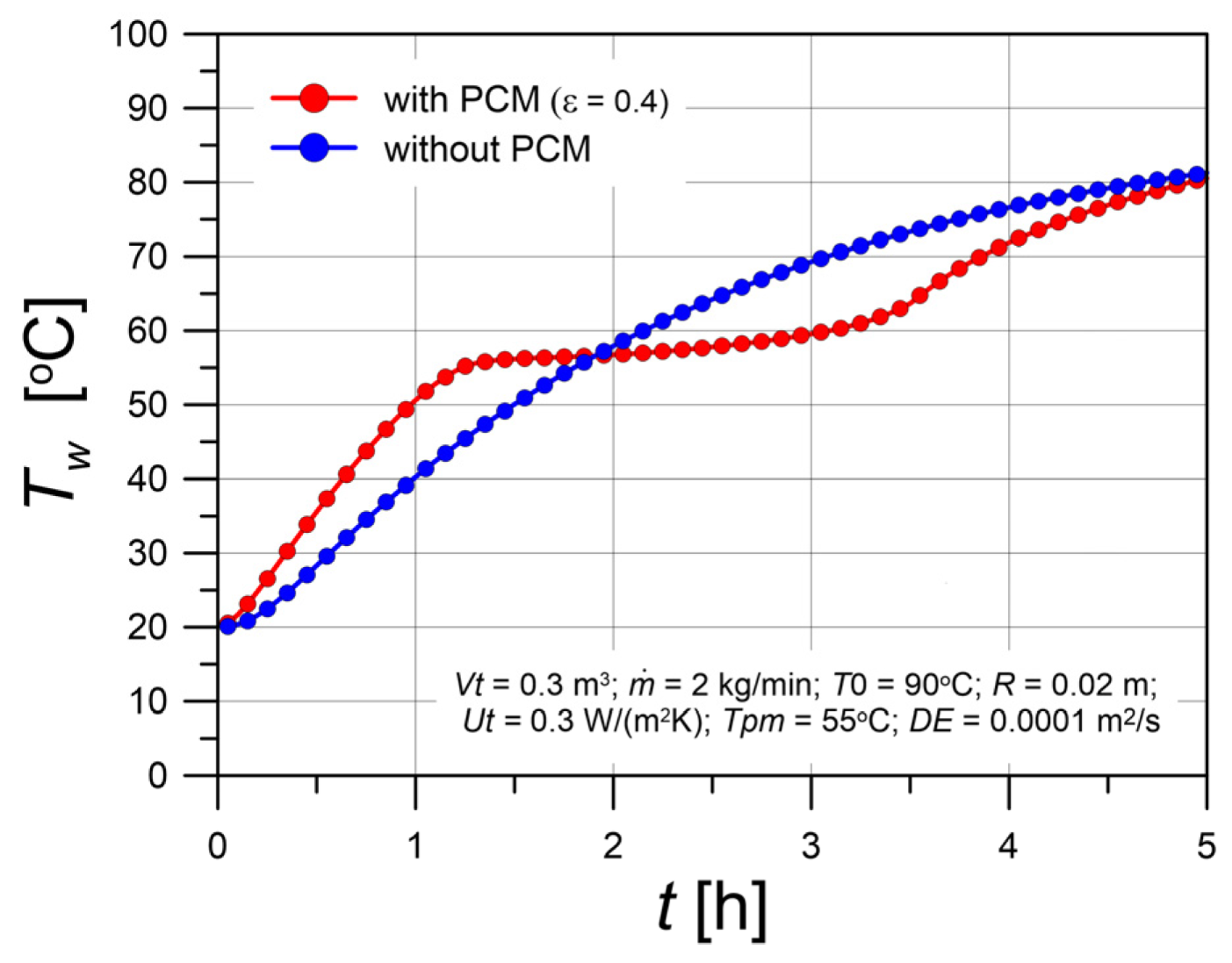
Figure 4 presents a comparison of the temporal outlet water temperature courses for the tank with PCM and the tank without PCM under identical operating conditions. For the tank without PCM, the temperature curve shows a smooth increase. In contrast, in the tank with PCM the temperature evolution consists of three stages. Initially, the water temperature increases, then remains at the PCM phase change temperature, and finally increases again. The constant water temperature occurs during the phase change of the PCM. Once the PCM has completely undergone phase transition (melted), the period of constant outlet water temperature ends.

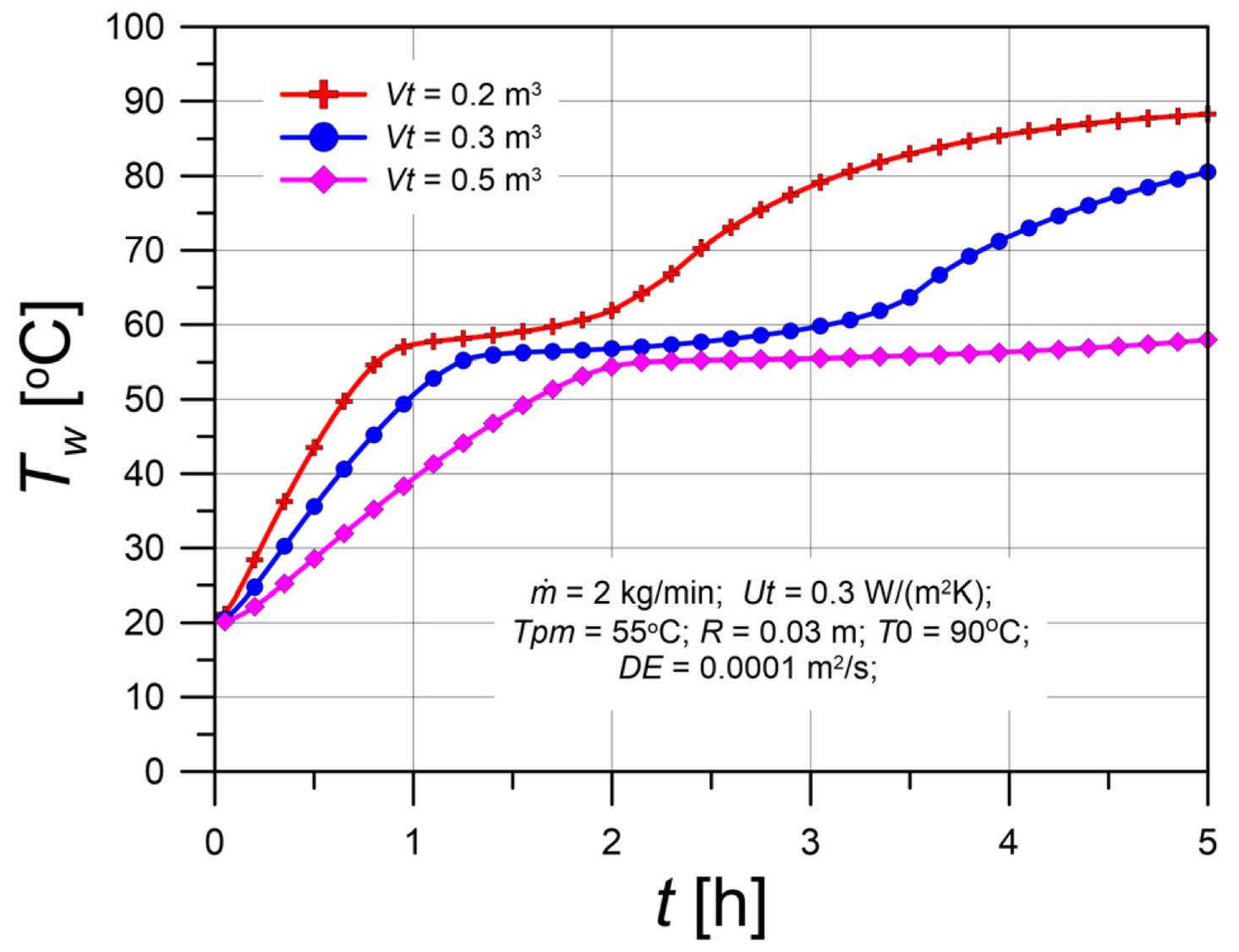
The tank volume $V_t$ has a strong influence on the process behavior. Temperature courses for different values of $V_t$ are shown in Figure 5. As the volume of the PCM-filled tank increases, the rise in outlet water temperature becomes slower. Consequently, for larger tank volumes, the phase change temperature is reached after a longer time. Since a larger tank contains more PCM, the thermal capacity of the PCM is higher, resulting in a longer period of temperature stabilization.

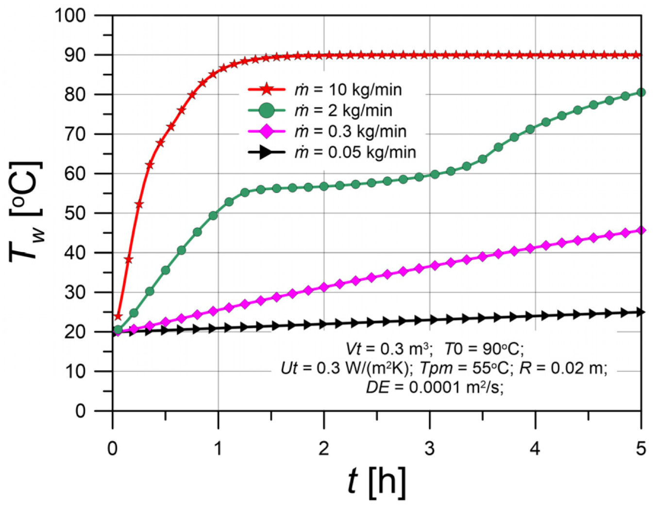
The water flow rate through the tank is another important factor. The obtained relationships are shown in Figure 6. For very high water flow rates, the presence of PCM has practically no effect on the outlet water temperature, which quickly reaches the inlet temperature of 90 °C. As the flow rate decreases, the influence of PCM becomes increasingly pronounced. For very low water flow rates, the effect of PCM appears only after long process durations, which are not shown in the figure.

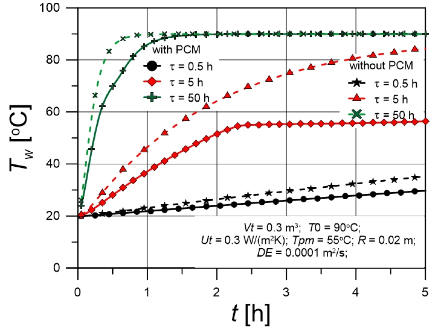
The mean residence time of water in the tank plays a key role in the heat storage process. The time course of the outlet temperature is influenced both by the fluid flow itself and by heat transfer between the water and the PCM. The mean residence time of a fluid in a flow-through tank is defined as the ratio of the tank volume to the volumetric flow rate:

$$\tau ={\displaystyle \frac{V}{{\rho }_w\stackrel{·}{m}}}$$

(23)

Figure 7 shows the temperature time courses for different mean residence times. When the tank is supplied with hot water, a longer residence time leads to a lower outlet temperature, which indicates a greater amount of heat stored in the system.

The residence time should be selected so that the thermal capacity of the PCM is used effectively. If the contact time is too short, the heat storage potential of the PCM is not fully utilized. On the other hand, excessively long residence times are impractical, as they require larger tank dimensions.

In the study by Wang et al. [17], outlet water temperature time courses were presented for a tank containing PCM (SAT) enclosed in steel tubes. During the heat absorption stage of the PCM, the experimental and simulated curves show strong similarity to those shown in Figure 7. The experimental study by Wang [17] was conducted over the temperature range of 30–91 °C, while the simulation calculations were performed using a CFD application.

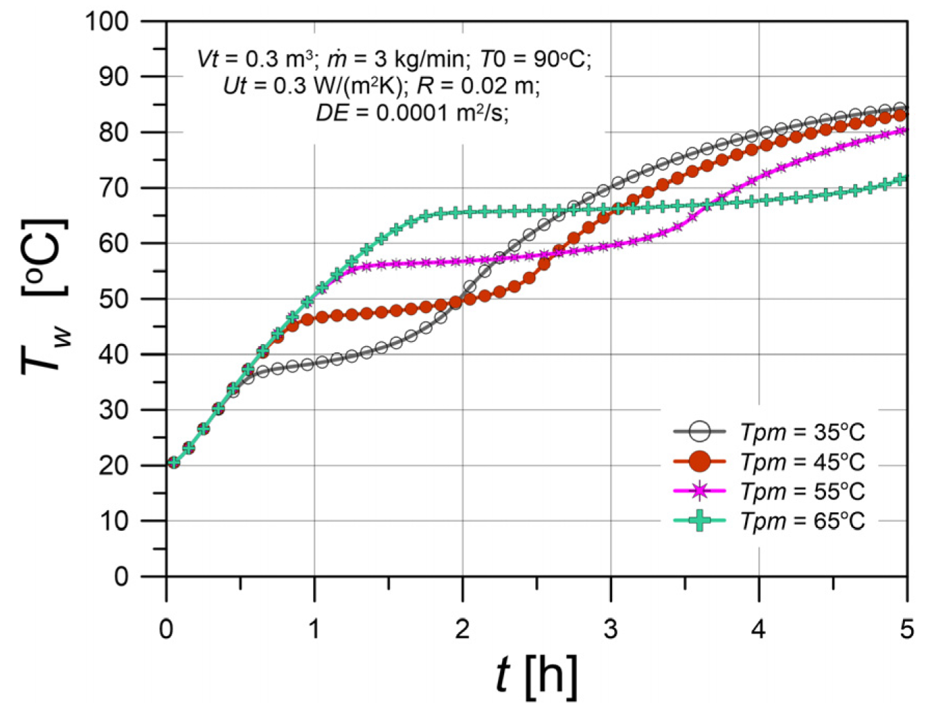
The primary parameter characterizing the PCM is the phase change temperature $T_{pm}$. Figure 8 shows the outlet water temperature courses for different values of $T_{pm}$. When the outlet water temperature is below $T_{pm}$, it increases with time. Once the water temperature reaches $T_{pm}$, it remains constant at this level. The duration of the temperature stabilization period depends on the value of $T_{pm}$. The higher the $T_{pm}$, the longer this period.

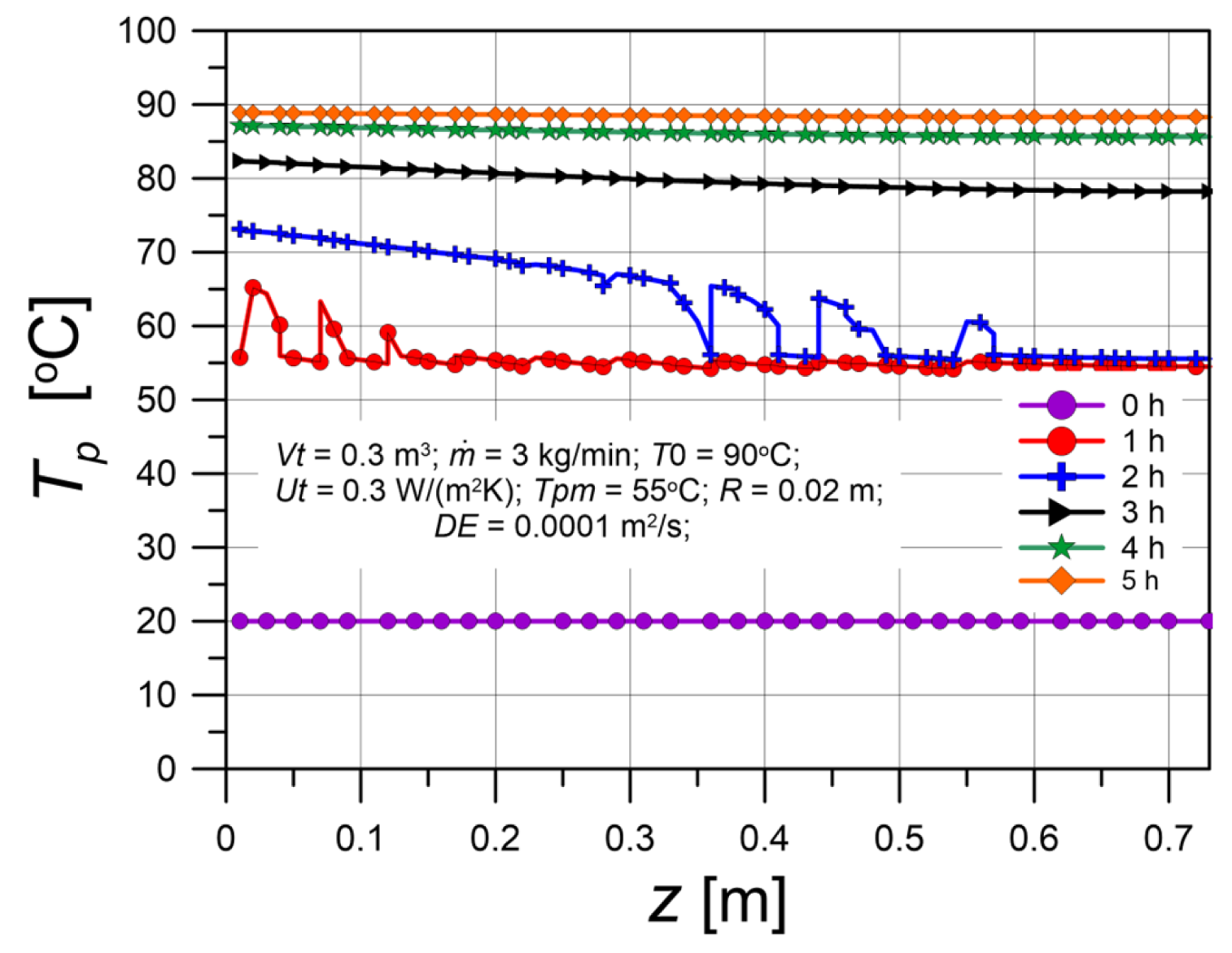
Figure 9 shows the PCM temperature variation along the position coordinate of the tank. At the initial stage, the temperature profile is uniform and corresponds to the initial condition of 20 °C. After 1 h, the PCM temperature is nearly uniform along the entire tank height and close to $T_{pm}$, indicating that the PCM is in a partially melted state. After the next hour, approximately half of the PCM volume near the inlet side of the tank has melted and is heated above $T_{pm}$. The subsequent profiles correspond to the liquid PCM state.

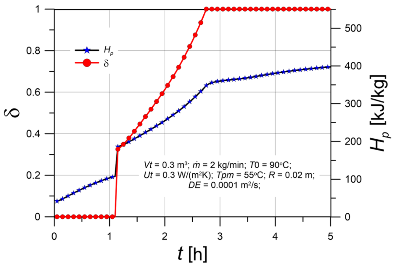
Figure 10 presents the time evolution of the liquid phase fraction in the PCM, $\delta$, and the PCM enthalpy, $H_p$, during the flow of hot water through the PCM-filled tank. The calculations were performed for a tank cross-section located at mid-height. The plot illustrates the heat absorption phase of the PCM. The temporal variation of $\delta$ consists of three stages: heating of solid PCM ($\delta =0$), melting of the PCM ($0<\delta <1$), and heating of liquid PCM ($\delta =1$). These three stages can also be identified in the time evolution of the PCM enthalpy, defined according to Equation (1).

The time course of the liquid phase fraction (SAT) was investigated by Bouhal et al. [21]. The numerically generated curve reported by these authors has a shape similar to that shown in Figure 10.

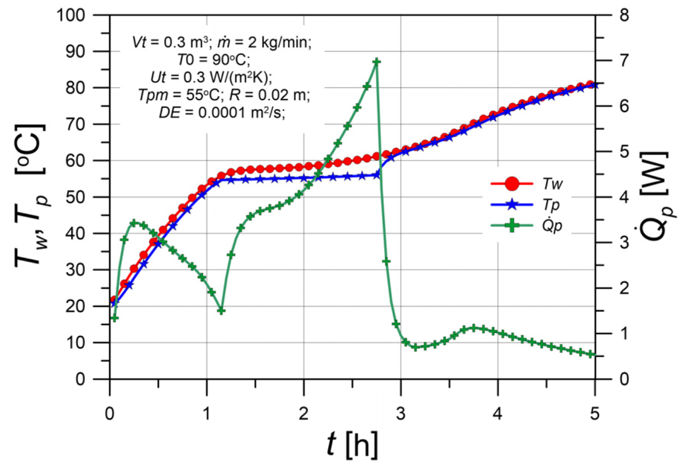
Figure 11 provides a further interpretation of the flow through the tank. As in the previous case, a tank cross-section at mid-height is considered. This stage corresponds to heating of the PCM; therefore, $T_w>T_p$, while in the final period the temperatures of both phases become nearly equal. The small differences between these temperatures indicate that heat transfer resistance does not play a dominant role in the process. This is partly due to the relatively long contact time between the water and the PCM. For known temperature values, the heat flux ${\stackrel{·}{Q}}_p$ can be calculated using Equation (5), and in this case (heating) it takes positive values. During the phase change period, a strong temporal variation of the transferred heat flux ${\stackrel{·}{Q}}_p$ is observed in the central part of the plot.

Temperature time courses for both water and PCM were presented by Kong et al. [22]. The shapes of the curves obtained in that study show strong similarity to the lines corresponding to T_w and T_p in Figure 11.

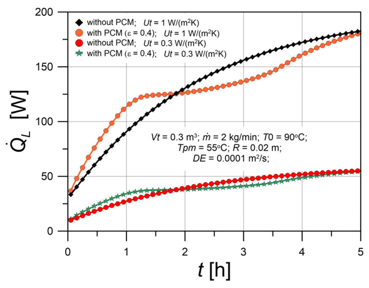
The model presented in this study accounts for heat losses to the surroundings. These losses depend on the overall heat transfer coefficient of the tank walls, $U_t$, which is mainly influenced by the thickness of the wall insulation. Figure 12 shows the heat flux lost to the surroundings as a function of time for different values of $U_t$. Relation (17) was used, and the average water temperature in the tank was calculated by integrating the temperature profile. For comparison, heat losses for a tank without PCM under the same conditions are also shown. The shapes of the curves for the PCM-filled tanks are similar to those of the outlet water temperature profiles (Figure 5). Under the simulated conditions, heat losses from the PCM-filled tank initially exceed those from the tank without packing; however, subsequently the losses from the PCM-filled tank become smaller. Consequently, the total amount of heat lost in both cases is comparable.

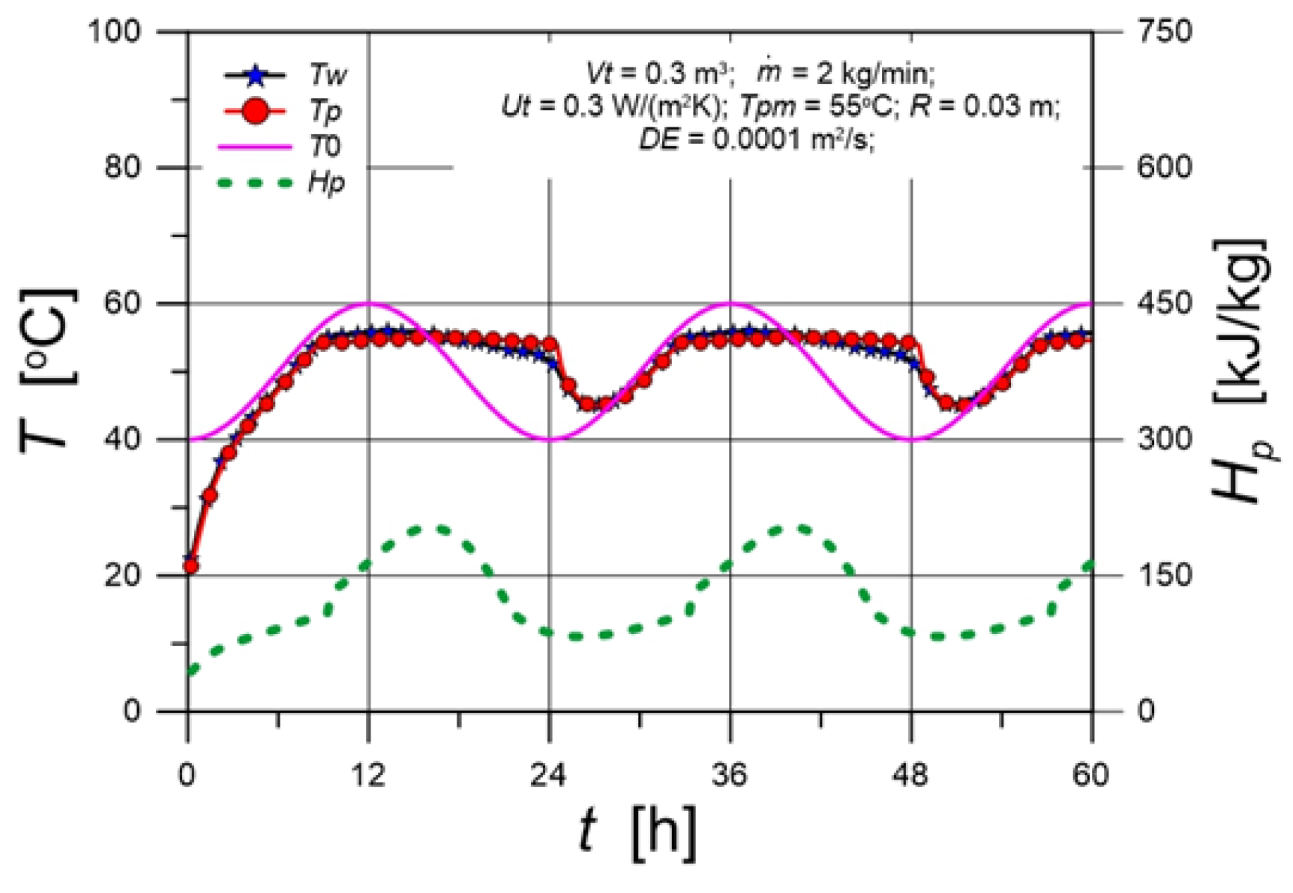
PCM-filled tanks operate in heating/cooling cycles to stabilize the outlet water temperature. This process was simulated by applying a cyclically varying inlet water temperature. The following functional form of the inlet water temperature was used:

$$T_0=50-10·\cos \left(\omega t\right)$$

(24)

where and $t$ denotes time [h]. The varying inlet water temperature induces cyclic changes in the direction of heat transfer between the water and the PCM. As a result, the heat stored in the PCM is subsequently released, and the cycle repeats. Depending on the operating parameters of the process, the presence of PCM may lead to partial or complete smoothing of the outlet temperature profile. Figure 13 illustrates an example of partial smoothing of temperature fluctuations. The use of PCM with a phase change temperature of T_pm = 55 °C limits the upper level of the outlet water temperature to this value, while simultaneously increasing the lower temperature level from 40 °C to approximately 45 °C. A phase shift of about 6 h between the inlet and outlet temperature curves is also observed. The figure additionally shows the PCM temperature at the extreme cross-section of the column on the outlet side, $T_p\left[n\right]$. For each process time, the instantaneous mean temperature of the PCM in the tank was calculated. The corresponding PCM enthalpy, H_p, was then determined using Equation (1). The resulting time course of the PCM enthalpy is shown in Figure 13 as a dashed line. This curve illustrates how the amount of stored heat evolves over time, as well as the associated time shift.

3.3. Longitudinal Dispersion in the Tank

Longitudinal mixing (dispersion) has a significant influence on the intensity of processes occurring in flow-through tanks. One way to account for this phenomenon is to introduce the concept of a longitudinal dispersion coefficient. This quantity is analogous to the thermal diffusivity coefficient. However, thermal diffusivity (as well as mass diffusivity) is a physical property, whereas the dispersion coefficient is a model parameter.

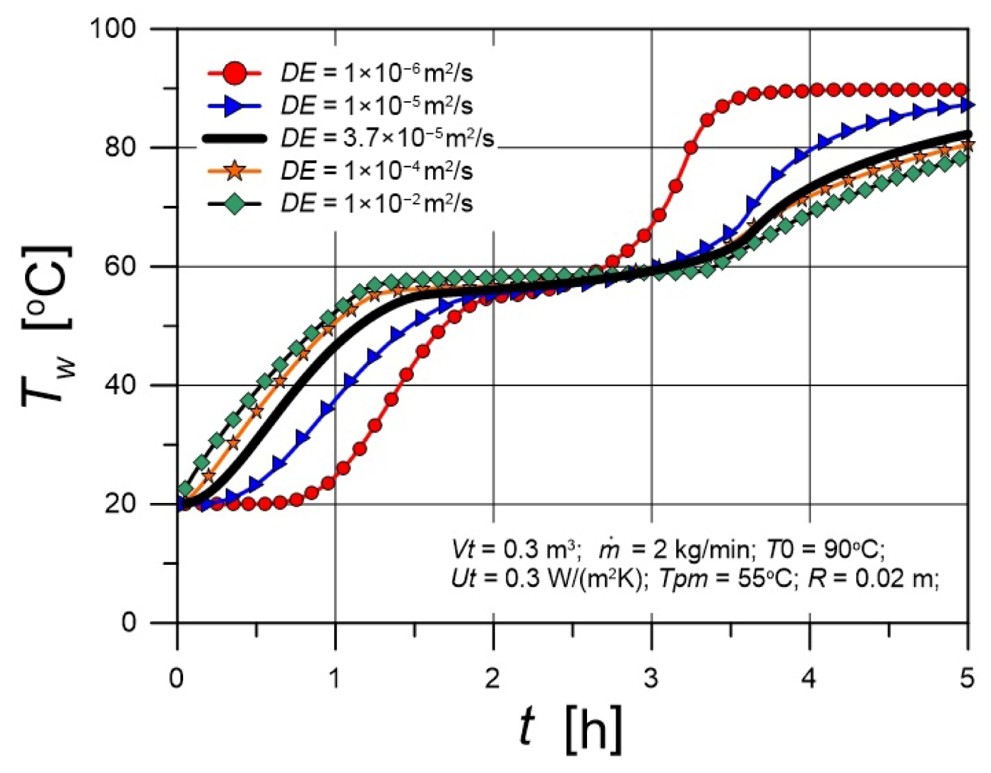
Figure 14 shows the effect of longitudinal dispersion on the outlet water temperature from the tank. The difference between the temperature profiles for the extreme values of $D_E$ is significant, indicating that the performance of the PCM strongly depends on the intensity of fluid mixing during flow through the tank. Mixing is unfavorable for heat transfer processes, as it leads to a reduction in the driving force of the process.

For the determination of the dispersion coefficient under liquid flow conditions through spherical packing, Wakao and Funazkri [30] proposed the following empirical correlation:

$$D_E={\displaystyle \frac{1}{\epsilon }}\left[\left(0.6÷0.8\right)a_w+Ru\right]$$

(25)

where a_w denotes the water thermal diffusivity and u represents its superficial velocity.

The dispersion coefficient was determined for flow through a packed bed composed of spheres with radius R = 0.02 m. For a cylindrical tank whose height equals its diameter, with a volume of 0.3 m³, and with water flowing at a mass flow rate of 2 kg/min, the velocity is 0.0805$·$10⁻³ m/s, corresponding to a Reynolds number of Re = 3.2. The bed porosity was assumed to be ε = 0.4. Using Equation (25), the resulting value is D_E = 3.7·10⁻⁵ m²/s (with the constant in Equation (25) taken as 0.7). In Figure 14, the solid line shows the outlet temperature profile corresponding to the above value of D_E.

Figure 15 illustrates the effect of longitudinal dispersion on the processes occurring in a flow-through tank. The upper curve corresponds to plug flow, while the lower one represents nearly perfectly mixed flow. The inlet water temperature is 90 °C, whereas the water temperature at z = 0 depends on the flow regime. Under plug flow conditions, the water temperature near the inlet is also 90 °C; however, when dispersion is significant, the temperature becomes more uniform along the tank position. In dispersive flow, the temperature step of the water at the inlet (in this case a decrease) reduces the driving force for heat transfer to the PCM compared to plug flow conditions.

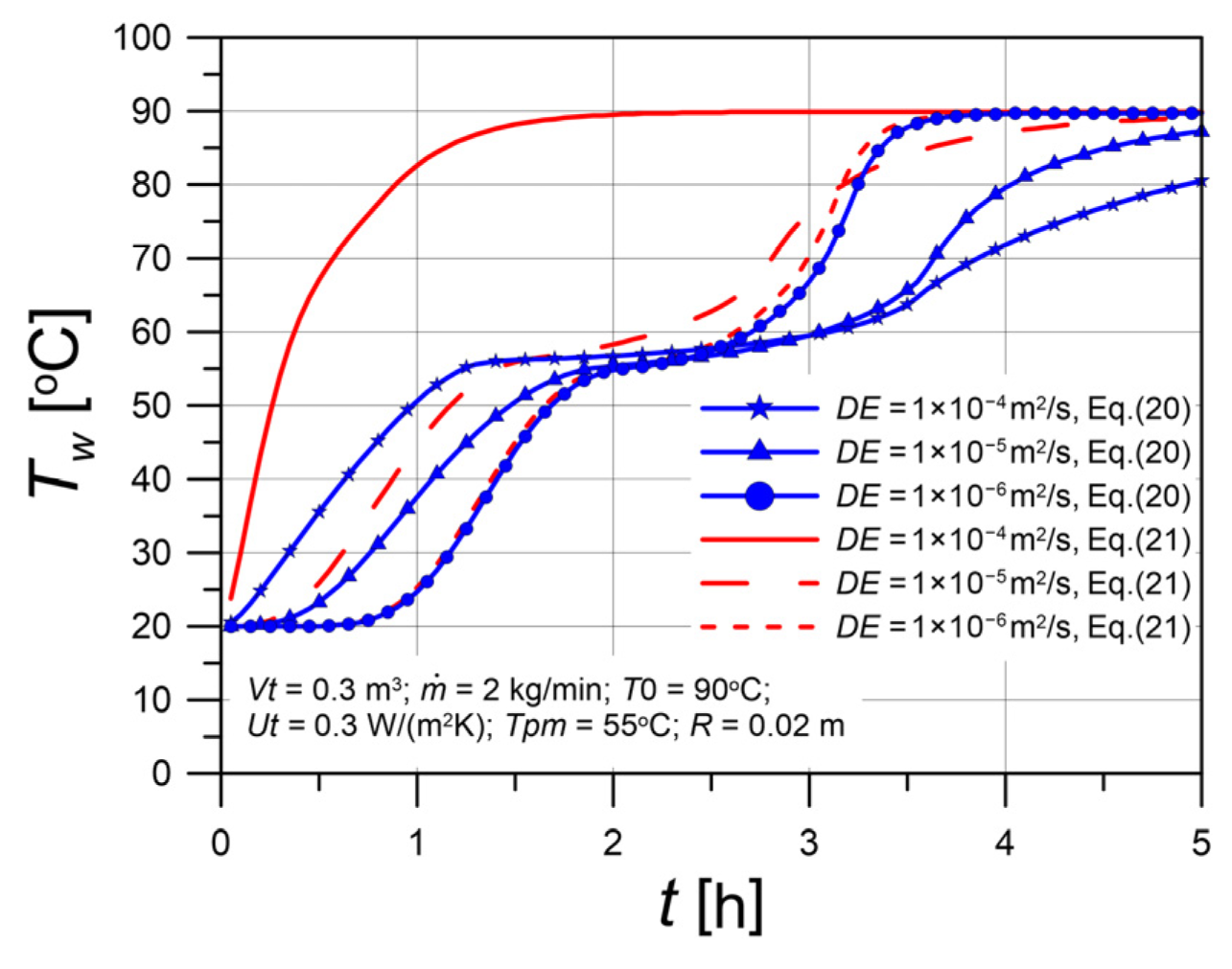
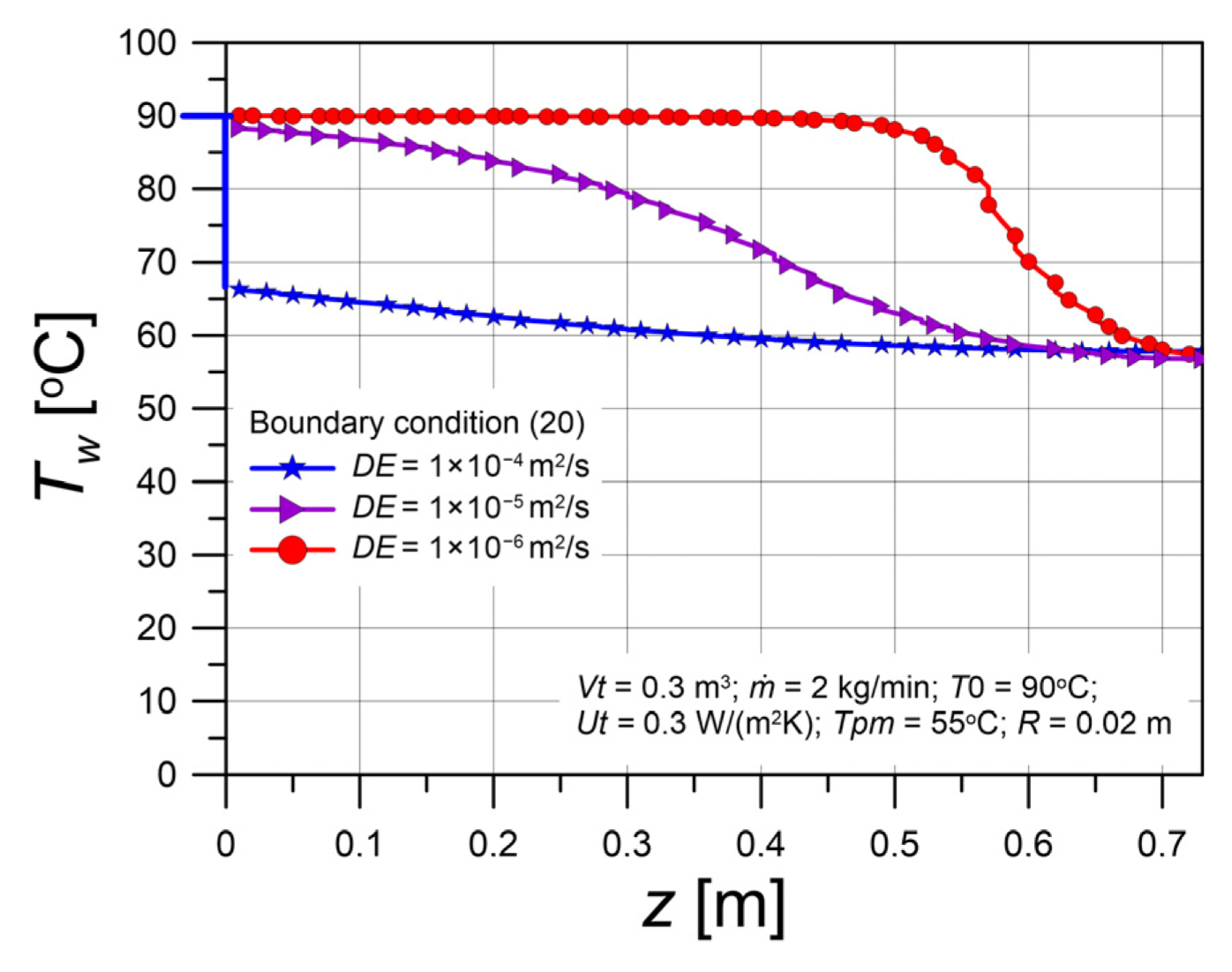
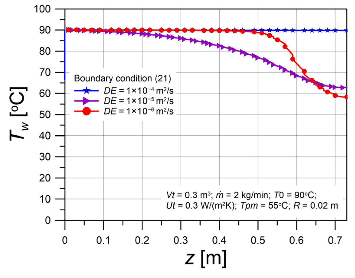
Figure 16 shows the temperature profiles of water in the tank when boundary condition (21) is applied. If the dispersion coefficient is small (e.g., 10⁻⁶ m²/s), the resulting temperature profile is identical to that shown in the previous figure. However, when dispersion is significant (e.g., 10⁻⁴ m²/s), the temperature profiles in the two figures differ substantially. Thus, condition (21) applies only to plug flow, whereas condition (20) has no restrictions regarding the dispersive character of the flow.

The Peclet number for dispersive flow is a dimensionless parameter that characterizes the ratio of the convective flux to the dispersive flux. The Peclet number is defined as follows:

$$Pe={\displaystyle \frac{uL}{D_E}}$$

(26)

where L is the characteristic length. For flow through spherical packing, L = 2R. The modified Peclet number, Pe_L, is based on the tank height L_t as the characteristic length. High values of Pe_L indicate that convective transport dominates over dispersion, whereas low values indicate the opposite. The limiting values of the Peclet number corresponding to ideal mixing and plug flow are 0 and $\infty$, respectively. In practice, however, flow is considered to approach ideal mixing for Pe_L < 2, while plug flow conditions are typically assumed for Pe_L > 50.

For the conditions used in the simulations, the values of the modified Peclet number were evaluated for different values of the dispersion coefficient. For values used in the calculations, the following result was obtained: L_t = 0.726 m, which gives:

• For D_E = 1·10⁻⁶ m²/s, the Peclet number is: Pe_L = 58, corresponding to plug flow.
• For D_E = 1·10⁻⁴ m²/s, the Peclet number is: Pe_L = 0.58, corresponding to ideally mixed flow.

Figure 17 presents calculation results confirming the necessity of applying boundary condition (20) when the flow is dispersive. The calculations were carried out for D_E = 1·10⁻⁴, D_E = 1·10⁻⁵, and D_E = 1·10⁻⁶ m²/s. The curves with symbols correspond to the Danckwerts boundary condition (20), whereas the curves without symbols correspond to the simplified condition (21). For D_E = 1·10⁻⁶ m²/s, the choice of boundary condition is practically insignificant. This value corresponds to Pe_L = 58, indicating plug-flow conditions. However, for D_E = 1·10⁻⁴ m²/s, the difference between the outlet water temperature time courses calculated using the two boundary conditions is very large. This value corresponds to Pe_L = 0.58, indicating flow close to ideal mixing. In this case, the use of condition (21) leads to results that are inconsistent with the actual physical behavior. Similarly, for D_E = 1·10⁻⁵ m²/s, the application of condition (21) also leads to noticeable errors.

3.4. Heat Transfer in a Spherical Packing Element

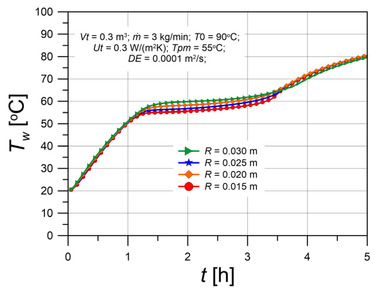
The thermal resistance between the water and the PCM is concentrated within the packed-bed elements. This resistance is mainly influenced by the thermal conductivity of the PCM and the radius of the spherical bed elements. Figure 18 shows the outlet water temperature profiles as a function of the radius $R$ of the spherical bed elements. Differences between the temperature courses for various values of $R$ appear mainly during the phase change period. Larger bed elements correspond, according to relation (13), to a lower heat transfer coefficient. Under these conditions, the hot water stream cools more slowly and maintains a higher temperature compared to the case of smaller spherical elements.

A preliminary comparison was performed between experimental and calculated values of the heat transfer coefficient between the shell and the interior of the packing element containing the encapsulated PCM. Kong et al. [22] report a value indicating that, during the discharging period, h = 40 W/(m²K). This value refers to a cylindrical element with a radius of 0.0138 m. For comparison, a relation derived from the linear driving force (LDF) model was used. An expression analogous to Equation (15) was applied; for a cylinder, the constant in Equation (15) equals 4.

A key difficulty lies in determining an appropriate value of the PCM thermal conductivity.

Table 2. Thermal conductivity of PCM materials, k_p [W/(mK)].

PCM	Value	Source
SAT	0.34–0.55	Wang [17]
SAT	0.5	Kong et al. [22]
Paraffin RT35HC	0.2	Bianqui et al. [14]

shows a wide scatter of reported values, most likely resulting from the use of different additives intended to enhance the thermal conductivity of the PCM. The calculations yield heat transfer coefficients in the range of 58–145 W/(m²K). Thus, the LDF equation leads to overestimated values of h, suggesting that an effective thermal conductivity, determined empirically, should be used instead. It is also worth noting that, for the charging period, the values of h reported by Kong et al. [22] are several times lower than those for the discharging period.

4. Conclusions

• The inclusion of longitudinal dispersion in the model equations enables a more accurate description of heat transfer in a flow-through tank containing PCM elements.
• The application of the Linear Driving Force (LDF) equation substantially simplifies the heat transfer model. Considering the complexity of phase change processes in confined domains, the use of an approximate LDF relation is justified and does not compromise the model accuracy.
• The LDF equation applied in the model for spherical elements can be extended to other packing geometries, such as cylinders or plates.
• Despite the applied simplifications, the proposed model correctly captures the system behavior and allows for a reliable evaluation of the influence of key process parameters. A limitation of the proposed model is that it does not account for the supercooling of the PCM during cooling processes.
• The proposed model enables systematic analysis of the influence of key design and operating parameters, including tank volume, water flow rate, PCM melting temperature, axial dispersion intensity, and PCM capsule size. Owing to its moderate computational cost, the model offers an intermediate-level approach between high-fidelity CFD simulations and simplified system-level models. While further experimental validation and improved estimation of heat transfer and dispersion parameters are required, the model can support preliminary performance assessment and parametric design studies of PCM-enhanced solar water heating systems.
• Simulation calculations based on the model were carried out to demonstrate its potential applicability to practical problems.

References

1. Li, Z.; Ma, T.; Zhao, J.; Song, A.; Cheng, Y. Experimental study and performance analysis on solar photovoltaic panel integrated with phase change material. Energy 2019, 178, 471–486. [Google Scholar] [CrossRef]
2. Yuan, W.; Ji, J.; Modjinou, M.; Zhou, F.; Li, Z.; Song, Z.; Huang, S.; Zhao, X. Numerical simulation and experimental validation of the solar photovoltaic/thermal system with phase change material. Appl. Energy 2018, 232, 715–727. [Google Scholar] [CrossRef]
3. Amalu, E.H.; Fabunmi, O.A. Thermal control of crystalline silicon photovoltaic (c-Si PV) module using docosane phase change material (PCM) for improved performance. Sol. Energy 2022, 234, 203–221. [Google Scholar] [CrossRef]
4. Duan, S.; Wang, L.; Zhao, Z.; Zhang, C. Experimental study on thermal performance of an integrated PCM Trombe wall. Renew. Energy 2021, 163, 1932–1941. [Google Scholar] [CrossRef]
5. Abdullah, A.A.; Atallah, F.S.; Ahmed, O.K.; Daoud, R.W. Performance improvement of photovoltaic/Trombe wall by using phase change material: Experimental assessment. J. Energy Storage 2022, 55, 105596. [Google Scholar] [CrossRef]
6. Kong, X.; Li, J.; Fan, M.; Li, W.; Li, H. Study on the thermal performance of a new double layer PCM Trombe wall with multiple phase change points. Sol. Energy Mater. Sol. Cells 2022, 240, 111685. [Google Scholar] [CrossRef]
7. Larwa, B.; Cesari, S.; Bottarelli, M. Study on thermal performance of a PCM enhanced hydronic radiant floor heating system. Energy 2021, 225, 120245. [Google Scholar] [CrossRef]
8. Cesari, S.; Emmi, G.; Bottarelli, M. A weather forecast-based control for the improvement of PCM enhanced radiant floors. Appl. Therm. Eng. 2022, 206, 118119. [Google Scholar] [CrossRef]
9. Wang, P.; Liu, Z.; Xi, S.; Zhang, Y.; Zhang, L. Experiment and numerical simulation of an adaptive building roof combining variable transparency shape-stabilized PCM. Energy Build. 2022, 263, 112030. [Google Scholar] [CrossRef]
10. Shi, Y.; Zhao, Y.; Zhang, Y.; Jiang, D.; Fan, Z. Experimental study of the thermal insulation performance of phase-change ventilated roofs. Energy Build. 2024, 303, 113819. [Google Scholar] [CrossRef]
11. Li, D.; Zheng, Y.; Liu, C.; Wu, G. Numerical analysis on thermal performance of roof contained PCM of a single residential building. Energy Convers. Manag. 2015, 100, 147–156. [Google Scholar] [CrossRef]
12. Cabeza, L.F.; Nogués, M.; Roca, J.; Illa, J.; Hiebler, S.; Mehling, H. PCM-module to improve hot water heat stores with stratification: First tests in a complete solar system. In Proceedings of the 9th International Conference on Thermal Energy Storage, Warsaw, Poland, 1–4 September 2003. [Google Scholar]
13. Mehling, H.; Cabeza, L.F.; Hippeli, S.; Hiebler, S. PCM-module to improve hot water heat stores with stratification. Renew. Energy 2003, 28, 699–711. [Google Scholar] [CrossRef]
14. Bianqui, C.; Viedma, A.; Egea, A.; García, A. Experimental analysis of the melting and solidification patterns in a PCM encapsulation for domestic hot water production. Appl. Therm. Eng. 2025, 272, 126313. [Google Scholar] [CrossRef]
15. Dannemand, M.; Johansen, J.B.; Kong, W.; Furbo, S. Experimental investigations on cylindrical latent heat storage units with sodium acetate trihydrate composites utilizing supercooling. Appl. Energy 2016, 177, 591–601. [Google Scholar] [CrossRef]
16. Wang, G.; Dannemand, M.; Xu, C.; Englmair, G.; Furbo, S.; Fan, J. Thermal characteristics of a long-term heat storage unit with sodium acetate trihydrate. Appl. Therm. Eng. 2021, 187, 116563. [Google Scholar] [CrossRef]
17. Wang, G.; Xu, C.; Englmair, G.; Kong, W.; Fan, J.; Furbo, S.; Wei, G. Experimental and numerical study of a latent heat storage using sodium acetate trihydrate for short- and long-term applications. J. Energy Storage 2022, 47, 103588. [Google Scholar] [CrossRef]
18. Koželj, R.; Mlakar, U.; Zavrl, E.; Stritih, U.; Stropnik, R. An experimental and numerical analysis of an improved thermal storage tank with encapsulated PCM for use in retrofitted buildings for heating. Energy Build. 2021, 248, 111196. [Google Scholar] [CrossRef]
19. Pop, O.G.; Balan, M.C. A numerical analysis on the performance of DHW storage tanks with immersed PCM cylinders. Appl. Therm. Eng. 2021, 197, 117386. [Google Scholar] [CrossRef]
20. Najafian, A.; Haghighat, F.; Moreau, A. Integration of PCM in domestic hot water tanks: Optimization for shifting peak demand. Energy Build. 2015, 106, 59–64. [Google Scholar] [CrossRef]
21. Bouhal, T.; El Rhafiki, T.; Kousksou, T.; Jamil, A.; Zeraouli, Y. PCM addition inside solar water heaters: Numerical comparative approach. J. Energy Storage 2018, 19, 232–246. [Google Scholar] [CrossRef]
22. Kong, W.; Wang, G.; Englmair, G.; Nielsen, E.N.N.; Dragsted, J.; Furbo, S.; Fan, J. A simplified numerical model of PCM water energy storage. J. Energy Storage 2022, 55, 105425. [Google Scholar] [CrossRef]
23. Tay, N.H.S.; Belusko, M.; Liu, M.; Bruno, F. Investigation of the effect of dynamic melting in a tube-in-tank PCM system using a CFD model. Appl. Energy 2015, 137, 738–747. [Google Scholar] [CrossRef]
24. Danckwerts, P.V. Continuous flow systems: Distribution of residence times. Chem. Eng. Sci. 1953, 2, 3857–3866. [Google Scholar] [CrossRef]
25. Seader, J.D.; Henley, E.J. Separation Process Principles; Wiley: Hoboken, NJ, USA, 2006; pp. 334–337. [Google Scholar]
26. Glueckauf, E. Theory of chromatography. Part 10. Formulae for diffusion into spheres and their application to chromatography. Trans. Faraday Soc. 1955, 51, 1540–1551. [Google Scholar] [CrossRef]
27. Liaw, C.H.; Wang, J.S.P.; Greencorn, R.A.; Chao, K.C. Kinetics of fixed-bed adsorption: A new solution. AIChE J. 1979, 25, 376–381. [Google Scholar] [CrossRef]
28. Georgiou, A.; Kupiec, K. Nonlinear driving force approximation for intraparticle mass transfer in adsorption processes. Nonlinear isotherm systems with macropore diffusion control. Chem. Eng. J. 2003, 92, 185–191. [Google Scholar] [CrossRef]
29. Duffie, J.A.; Beckman, W.A. Solar Engineering of Thermal Processes; Wiley: Hoboken, NJ, USA, 2013. [Google Scholar] [CrossRef]
30. Wakao, N.; Funazkri, T. Effect of fluid dispersion coefficients on particle-to-fluid mass transfer coefficients in packed beds: Correlation of Sherwood numbers. Chem. Eng. Sci. 1978, 33, 1375–1384. [Google Scholar] [CrossRef]
Figure 1. Relationship between enthalpy and temperature for PCM.
Buildings 16 01172 g001
Figure 2. Flow-through tank with a packed bed of PCM elements.
Buildings 16 01172 g002
Figure 3. Heat fluxes in the PCM-filled tank.
Buildings 16 01172 g003
Figure 4. Temporal outlet water temperature courses for the tank with a PCM bed and without PCM.
Buildings 16 01172 g004
Figure 5. Effect of tank volume on the temporal outlet water temperature courses.
Buildings 16 01172 g005
Figure 6. Effect of water flow rate on the temporal outlet water temperature courses.
Buildings 16 01172 g006
Figure 7. Temperature time courses for different mean residence times.
Buildings 16 01172 g007
Figure 8. Effect of the phase change temperature T p m on the temporal outlet water temperature courses.
Buildings 16 01172 g008
Figure 9. PCM temperature profiles in the tank at different flow durations.
Buildings 16 01172 g009
Figure 10. Liquid phase fraction in the two-phase mixture and PCM enthalpy.
Buildings 16 01172 g010
Figure 11. Temporal variations of temperatures T w and T p and the heat flux Q · p between water and PCM.
Buildings 16 01172 g011
Figure 12. Heat losses in the PCM-filled tank.
Buildings 16 01172 g012
Figure 13. PCM heating/cooling cycles.
Buildings 16 01172 g013
Figure 14. Effect of the dispersion coefficient on the temporal outlet temperature courses of the tank.
Buildings 16 01172 g014
Figure 15. Water temperature profiles for boundary condition (20).
Buildings 16 01172 g015
Figure 16. Water temperature profiles for boundary condition (21).
Buildings 16 01172 g016
Figure 17. Effect of the boundary condition on the outlet water temperature time courses.
Buildings 16 01172 g017
Figure 18. Effect of the PCM bed element radius on the temporal outlet water temperature courses.
Buildings 16 01172 g018