Electrical Resistivity-Based Prediction of Corrosion-Affected Areas in Reinforced Concrete

Abstract

This study investigates the development of a predictive model in simulations for assessing steel corrosion in determining corrosion-affected zones in reinforced concrete. A series of reinforced concrete cubes with varying degrees of corrosion were tested using a four-probe Wenner configuration. The experimental data showed a clear inverse relationship between ER and steel mass loss, with a strong negative correlation, highlighting the potential of ER as a corrosion indicator. A third-degree polynomial model was developed to predict the diameter of the corrosion-affected region based on steel mass loss and concrete cover, achieving high predictive accuracy. This model was validated using numerical simulation conducted in COMSOL Multiphysics, which replicated the experimental setup under steady-state conditions. Parametric studies further examined the effects of electrical conductivity ($\sigma$) and electrode spacing on the simulated results. The findings confirm that while $\sigma$ has a moderate impact, electrode spacing significantly influences the measured ER values. The study underscores the importance of incorporating variable parameters into simulation models to improve the accuracy and field applicability of ER-based corrosion assessments. Furthermore, the simulation framework developed in this study demonstrates how numerical modeling can enhance the interpretive value of ER measurements, supporting the advancement of non-destructive testing techniques aimed at improving corrosion monitoring and maintenance strategies.

1. Introduction

Reinforced concrete (RC) is the cornerstone material in modern infrastructure due to its versatility, strength, and cost-effectiveness [1]. However, the long-term performance of RC structures is significantly influenced by their durability under service conditions [1,2]. Durability, defined as the ability of concrete to resist weathering action, chemical attack, and abrasion while maintaining its desired engineering properties, is a critical aspect of sustainable infrastructure [3,4,5]. Over time, aggressive environmental agents, particularly chlorides, sulfates, and carbon dioxide, penetrate concrete and initiate various forms of deterioration [6]. As deterioration progresses, evaluating the in-situ condition of RC becomes essential to plan maintenance, repair, or rehabilitation. Durability evaluation techniques must be capable of detecting early signs of degradation to avoid costly failures and extend the service life of structures [5,7,8].

Among the different degradation mechanisms, chloride-induced corrosion is one of the most prevalent and damaging forms, particularly in marine environments and areas exposed to de-icing salts. Chloride ions permeate the concrete cover and accumulate at the steel–concrete interface, disrupting the passive oxide layer that protects steel reinforcement. Once degraded, steel undergoes active corrosion, producing expansive rust that includes tensile stresses in the surrounding concrete [9,10,11,12]. This results in cracking, spalling, and delamination, and ultimately compromises structural performance. The time between chloride ingress and the onset of visible damage can vary widely, making early detection and monitoring of corrosion activity a vital component of structural durability management [13,14,15].

Corrosion of reinforcement not only reduces the cross-sectional area of steel but also leads to significant deterioration of the surrounding concrete matrix, a critical factor affecting structural performance and durability [16,17,18,19,20,21]. As steel corrodes, the expansive nature of the rust products exerts internal pressure on the adjacent concrete, resulting in radial cracking, delamination, and eventually spalling of the concrete cover [7,9]. This localized damage compromises the protective barrier of the concrete, accelerating further ingress of chlorides, moisture, and oxygen, which perpetuates the corrosion cycle. Experimental observations have shown that even low levels of corrosion can initiate visible cracking and material degradation around the rebar, reducing the structural capacity and service life of RC elements [22,23]. As the concrete deteriorates, the confinement around the steel is weakened, increasing the susceptibility of the member to deformation, cover detachment, and premature failure under load.

To evaluate the in-situ condition of RC structures without compromising their integrity, non-destructive testing (NDT) methods are increasingly employed. NDT techniques offer a practical means to detect defects, assess material properties, and monitor deterioration processes. Widely used methods include ultrasonic pulse velocity (UPV), rebound hammer, half-cell potential mapping, ground-penetrating radar (GPR), and electrical measurements [24,25,26]. These methods help engineers and inspectors obtain diagnostic data rapidly and cost-effectively, supporting decisions related to maintenance and rehabilitation. Among these, electrical techniques, particularly electrical resistivity (ER), have shown promise for evaluating parameters closely related to durability, such as permeability, moisture content, and corrosion activity [13,27,28,29].

Electrical resistivity (ER) refers to the ability of concrete to resist the flow of electrical current and is influenced by factors such as water-to-binder ratio [30,31], mixture composition [32], curing conditions, age of the concrete [33,34], degree of saturation [35,36,37], specimen geometry [38], microstructure properties (such as pore size and volume) [39], chloride content, surface-breaking cracks [40,41], and the presence of steel reinforcements [42,43,44,45]. It provides a non-invasive means to estimate the corrosion risk of embedded steel reinforcement, as lower resistivity values are typically associated with a higher probability of active corrosion [46,47,48]. ER measurements can be conducted on the surface of concrete structures using a four-point Wenner probe, allowing rapid and repeatable assessments. In this setup, four electrodes were arranged in a straight line, each spaced equidistantly by a distance ‘s,’ as illustrated in Figure 1 [15,49,50,51]. Due to its simplicity, cost-effectiveness, and proven correlation with corrosion processes, ER is increasingly used in both field inspections and laboratory studies focused on concrete durability [52,53].

Recent studies have further advanced the understanding of corrosion monitoring and electrical resistivity-based assessment in reinforced concrete. Electrical resistivity measurements combined with numerical simulations can quantify corrosion-induced electrical field distortion [54]. Data-driven approaches using machine learning have been introduced to detect early corrosion damage based on non-destructive testing signals, indicating a shift toward hybrid experimental-computational frameworks [55]. More recently, the impact of internal cracking and reinforcement geometry on electrical resistivity distribution through numerical modeling was investigated [56]. In addition, multi-physics and coupled electrochemical models have been proposed to improve corrosion prediction accuracy in reinforced concrete [57,58]. Despite these advancements, most contemporary studies primarily address corrosion initiation, corrosion probability, or corrosion rate estimation. Quantitative prediction of the spatial extent of corrosion-affected zones in concrete using surface electrical resistivity remains largely unexplored, which motivates the present study.

Previous studies have quantitatively demonstrated the sensitivity of electrical resistivity (ER) measurements obtained using the four-point Wenner probe to corrosion activity in reinforced concrete. Concrete resistivity values below 10 kΩ·cm are typically associated with a high probability of active corrosion, whereas resistivity values exceeding 20 kΩ·cm indicate low corrosion risk [13]. An inverse relationship between ER and corrosion rate was observed, with resistivity decreasing from approximately 15 kΩ·cm to below 5 kΩ·cm as corrosion progressed under chloride exposure [14]. A strong correlation between ER and corrosion current density, with coefficients of determination (R²) exceeding 0.80 for chloride-contaminated reinforced concrete specimens was also identified [52]. It is then demonstrated that ER measurements reflect pore connectivity and ionic transport properties that govern corrosion kinetics [53]. These findings confirm that Wenner probe ER measurements are effective indicators of corrosion activity; however, most previous studies focus on corrosion initiation and rate assessment rather than quantifying the spatial extent of corrosion-affected zones within concrete.

Theoretically, ER is defined as the product of a geometric constant, k, and the ratio of the measured electric potential difference (V) to the applied electric current (I). This relationship can be mathematically represented as:

$$\rho =\left({\displaystyle \frac{V}{I}}\right)\times k$$

(1)

Despite the established use of electrical resistivity (ER) in identifying corrosion activity and assessing general concrete quality, its integration into simulation-based approaches for modeling corrosion progression in reinforced concrete remains limited. Most existing studies associate ER primarily with electrochemical properties such as corrosion initiation, chloride ingress, and moisture content [59,60] but seldom incorporate ER data into numerical models that simulate the physical and structural consequences of corrosion over time. While corrosion-induced deterioration has been widely observed to affect both steel and surrounding concrete, there is a lack of comprehensive simulation frameworks that use ER as an input or validation parameter to predict the extent and severity of corrosion damage [61,62,63,64]. Given that the ER reflects changes in the internal condition of concrete, including pore connectivity and ionic movement, it presents an untapped opportunity to inform and enhance predictive modeling. However, the absence of validated methodologies linking ER measurements with corrosion simulation restricts its use in developing accurate service-life prediction models and structural diagnostics.

This study aims to develop and validate a simulation model that links electrical resistivity (ER) measurements to the extent of corrosion-induced damage in reinforced concrete (RC) structures. Specifically, the objectives are to: (1) evaluate the correlation between electrical resistivity values and actual steel mass loss under accelerated corrosion conditions; (2) simulate the electrical response of corroded RC specimens using COMSOL Multiphysics v6.2; (3) quantify the diameter of corrosion-affected concrete regions; and (4) identify the most suitable mathematical relationship that relates corrosion level, concrete cover depth, and corroded zone size. Ultimately, the study seeks to demonstrate the viability of ER as a reliable non-destructive parameter for assessing reinforcement corrosion and informing structural durability evaluation.

To achieve these objectives, the study will involve several key tasks. Reinforced concrete cube specimens will first be prepared and subjected to accelerated corrosion using impressed current techniques, with steel mass loss classified at stages of 0%, 5%, 10%, 15%, 20%, and 25%. Electrical resistivity measurements will be performed using a four-point Wenner probe method to monitor changes corresponding to increasing corrosion levels. Steel mass loss will be quantified through cleaning, chemical treatment, and the application of Archimedes’ principle, providing a reference for corrosion severity. A three-dimensional numerical simulation model will then be constructed in COMSOL Multiphysics to simulate electrical current flow and potential fields within the concrete, accounting for different degrees of corrosion and concrete cover thickness. Numerical outputs will be validated against experimental ER readings, and multiple regression models will be developed to predict the diameter of corroded zones.

2. Experimental Program

2.1. Preparation of Concrete Specimens

The experimental setup consisted of 36 concrete cube specimens, each measuring 200 mm × 200 mm, and reinforcing steel bars (rebars) with a length of 235 mm and a diameter of 19 mm. Of each rebar, 135 mm was embedded centrally within the concrete specimen, resulting in an effective exposed surface area of 4176 mm² for corrosion testing. The specimens were cast using 20 mm thick wooden molds, through which the rebar was positioned horizontally via a pre-drilled opening on one side of the formwork. To prevent unintended corrosion outside the designated exposure zone, the unembedded portion of the rebar was coated with two layers of epoxy followed by one layer of urethane, after which the urethane-coated section was wrapped with polytetrafluoroethylene (PTFE) tape. Additionally, a 100 mm polyvinyl chloride (PVC) sleeve was installed to provide supplementary protection to the non-contact length of the rebar.

The geometry and configuration of the reinforced concrete specimens used in this study are illustrated in Figure 2. The figure shows the 200 mm × 200 mm concrete cube with a centrally embedded D19 reinforcing bar, the defined corrosion-exposed region, and the protective epoxy- and PVC-coated segments used to localize corrosion damage. This geometric configuration was adopted to ensure controlled corrosion development within a known region and to provide a consistent reference for both experimental measurements and numerical simulations.

Table 1. Concrete mix designs and material composition.

Concrete Mix	Design Strength	w/c Ratio	Water (kg/m3)	Cement (kg/m3)	Gravel (kg/m3)
Mix 1	18 MPa	0.585	168	287	898
Mix 2	24 MPa	0.507	170	335	956
Mix 3	40 MPa	0.346	166	480	993

presents the mix proportions and material properties of three concrete mixtures used in this study, each with varying design strengths and water-to-cement (w/c) ratios. Mix 1 has a design strength of 18 MPa and the highest w/c ratio of 0.585, indicating a lower-strength concrete. Mix 2, with a strength of 24 MPa and a w/c ratio of 0.507, represents a medium-strength mix. Mix 3 is the highest strength concrete at 40 MPa and has the lowest w/c ratio of 0.346, reflecting its denser composition. The unit weights of materials used (in kg/m³) vary accordingly: water ranges from 166 to 170, cement from 287 to 480, gravel from 898 to 993, sand from 720 to 957, and the air-entraining agent from 2.5 to 4.32. These variations reflect adjustments made to achieve different mechanical properties and workability for each mix. All mixes utilized Type I Portland cement and included a high-performance air-entraining agent to enhance durability.

2.2. Accelerated Corrosion and Steel Mass Loss Measurement

The concrete specimens were subjected to an impressed current technique to simulate controlled steel corrosion, as illustrated in Figure 3, following the procedures adopted in previous studies [65,66,67]. Each specimen was immersed in a 3% sodium chloride (NaCl) solution for seven days to achieve full saturation. During immersion, the top surface of each cube remained fully submerged in the solution. A stainless-steel mesh (SUS 316) was wrapped around the specimen’s lateral surfaces to serve as the cathode, while the embedded reinforcing steel bars acted as the anodes [65].

A direct current (DC) power source (ODA Programmable DC Power Supply-OPE-DI Series) supplied a constant voltage, with a maximum applied current of 1.05A. The positive terminal was connected to the rebar, while the negative terminal was linked to the stainless-steel mesh. The electrical current was continuously monitored using a (KEYSIGHT Truevolt Digital Multimeter, KEYSIGHT, Santa Rosa, CA, USA) and real-time corrosion behavior was recorded using LabVIEW 2016 software [68].

Corrosion levels in the 19 mm rebars were classified according to their theoretical mass loss, corresponding to 0%, 5%, 10%, and 20% corrosion stages. Visible crack formation was observed on the concrete surface following exposure to the impressed current, with increasing crack width and corrosion staining corresponding to higher corrosion levels, consistent with observations from related corrosion acceleration experiments [67].

The schematic diagram presents the setup used for the accelerated corrosion test. The system consisted of a DC power supply, an electrical current measuring unit, and a computer-based monitoring system. The concrete specimen was partially submerged in a 3% NaCl solution, with the steel reinforcement connected to the positive terminal (anode) and the stainless-steel mesh surrounding the specimen connected to the negative terminal (cathode). Electrical clamps were used to secure proper contact during testing [65,67].

Quantification of steel mass loss was conducted following the standard procedure outlined in ASTM G1—Standard Practice for Preparing, Cleaning, and Evaluating Corrosion Test Specimens [ASTM G1, 2017]. After extraction from the concrete cubes, the corroded rebars underwent ultrasonic cleaning followed by immersion in a sodium hydroxide (NaOH) solution to dissolve corrosion products. Residual rust was further removed through sandblasting and high-pressure air-jet cleaning, exposing the intact metallic surface [22].

As illustrated in Figure 2, the corroded region was limited to a 70 mm segment, while the remaining embedded portion was protected using epoxy coatings and PVC sleeves to prevent unwanted corrosion. The mass loss was evaluated using Archimedes’ principle of buoyancy [69]. The rebars were submerged in water up to the corroded segment (70 mm), and the volume of displaced water represented the volume of steel loss. Using the known density of steel, the corroded steel mass was calculated. The percentage mass loss (mL), representing the degree of corrosion, was determined by normalizing the measured mass loss to the original uncorroded rebar mass [70].

The steel mass loss percentage was computed using Equation (2) where $m_L$ is percentage steel mass loss (%), $m_{air}$ is mass of the rebar measured in air (g), m_w(L) is mass of the rebar partially immersed in water (g), m₀ is initial mass of the uncorroded rebar segment (g), and ρ_s and ρ_w are densities of steel and water, respectively. This equation quantifies the corrosion level by comparing the corroded rebar’s buoyant mass to its original uncorroded mass, thus providing an accurate measure of the extent of material degradation due to corrosion [69,70].

$$m_L=\left[1-{\displaystyle \frac{{(m}_{air}-m_w\left(\mathrm{L}\right)){\rho }_s}{m_0{\rho }_w}}\right]\times 100\%$$

(2)

2.3. Electrical Resistivity Measurements

Figure 4a,b illustrates the top and 3D views of the electrical resistivity (ER) measurements performed on the surface of the concrete specimens. A commercially available four-point Wenner probe with an electrode spacing of 38 mm was employed for all ER measurements, following established procedures [71,72,73]. During testing, an external current between 50 µA and 200 µA was applied to the concrete surface to overcome contact resistance between the electrodes and the specimen.

To investigate the influence of rebar corrosion on concrete resistivity, measurements were taken directly above the embedded steel reinforcement. Upon contact with the surface, the device displayed the apparent ER value (in kΩ-cm) on a digital screen. For each specimen, five consecutive readings were recorded and averaged to minimize experimental variability arising from surface irregularities.

All measurements were completed within 10 min after the specimens were removed from the NaCl solution. The surfaces were lightly dried using a damp cloth to maintain a 100% pore water saturation level. ER data were collected every 24 h from one specimen in each concrete mix group (MIX1, MIX2, and MIX3) reinforced with D19 rebars, targeting corrosion levels of 0% and 20%. Measurements began immediately upon immersion in the NaCl solution and continued throughout the accelerated corrosion testing period. Simultaneously, specimen mass was monitored to account for changes in moisture content during ER assessment [75,76].

In this study, three forms of electrical resistivity (ER) were evaluated: apparent, true, and relative ER [66,77]. The apparent ER refers to the direct reading obtained from the Wenner probe during surface measurement. Meanwhile, the true ER accounts for geometric and boundary effects and is determined by dividing the apparent ER by a geometric correction factor, which is typically derived from finite-element or numerical simulation models [66,78]. On the other hand, the relative ER quantifies the variation in resistivity resulting from corrosion and is defined as the ratio of the ER measured at a specific corrosion level to that of an uncorroded specimen.

Previous studies have reported that several factors, such as electrode configuration, probe spacing, rebar diameter, and orientation, can significantly influence ER readings [13,77,78,79,80]. In particular, the alignment and spacing of reinforcing bars can alter current flow paths within the concrete matrix, thereby reducing the measured resistivity values [79,81,82].

Accordingly, this study focuses on ER as a diagnostic indicator to evaluate the relationship between rebar corrosion and concrete degradation. The relative ER ${\mathsf{\alpha }}_{\mathsf{\rho }}\left(\mathsf{\theta }\right)$ is expressed as the normalized ratio between the ER at a given corrosion level, $\mathsf{\rho }\left(\mathsf{\theta }\right)$, and the ER of the uncorroded condition, $\mathsf{\rho }\left(0\right)$, as shown in Equation 1 where $\mathsf{\theta }$ denotes the corrosion level of the reinforcing steel [81]. Both ${\mathsf{\alpha }}_{\mathsf{\rho }}\left(\mathsf{\theta }\right)$ and $\mathsf{\rho }\left(0\right)$ were obtained from specimens having the same concrete composition, rebar diameter, and embedment configuration [71,82]. The baseline apparent ER values, measured prior to the application of impressed current, were 3.28 kΩ·cm for MIX 1, 3.69 kΩ·cm for MIX 2, and 6.19 kΩ·cm for MIX 3 [74].

$${\mathsf{\alpha }}_{\mathsf{\rho }}\left(\mathsf{\theta }\right)={\displaystyle \frac{\mathsf{\rho }\left(\mathsf{\theta }\right)}{\mathsf{\rho }\left(0\right)}}$$

(3)

3. Numerical Simulation

3.1. Principle and Physics

The numerical simulation in this study was conducted using the Electric Currents physics interface under the AC/DC Module of COMSOL Multiphysics v6.2, and was based on the fundamental principle of electrical conduction in heterogenous media, specifically modeling how the changing steel mass of embedded reinforcement bars affects electrical resistivity (ER) measurements in concrete. Using the Wenner four-electrode method, the study simulates the electric potential field within a concrete cube by applying a known current and solving Poisson’s equation, as expressed in the equation below:

$$Q_j=\left(\sigma \nabla V-J^e\right)\times -\nabla$$

(4)

where $\sigma$ is the electrical conductivity, the inverse of electrical resistivity (ER), $V$ is the electrical potential, $J^e$ is the externally applied electric current, and $Q_j$ signifies the current source term. The simulation employs a 3D finite element model, where concrete and steel are assigned their respective electrical properties, concrete as a high-resistivity medium and steel as a highly conductive one. This setup reveals how the presence, position, and steel mass of rebars distort the current flow paths, leading to reduced apparent ER values. The modeling accounts for various geometric and physical parameters, such as electrode spacing, concrete cover, and steel mass loss, to quantify and calibrate the diameter of the concrete surrounding the rebar, ultimately enabling more accurate assessment of concrete durability through corrected resistivity readings.

3.2. Geometry, Simulation Setup, and Input Parameters

Figure 5 outlines the workflow used to develop the electrical resistivity (ER) measurement simulation in COMSOL Multiphysics v6.2. In this simulation, a 3D finite element model was constructed to represent corroded reinforced concrete cubes with varying levels of steel mass loss, aiming to estimate the diameter of the corroded region. The model replicates the experimental conditions, specifically a 200 mm × 200 mm concrete cube containing a centrally placed 19 mm steel rebar [74]. Mesh refinement was achieved using a free triangular mesh, with finer elements concentrated at the steel–concrete interface to enhance computational accuracy. The minimum element size was set to 0.025 mm and the maximum element size was set to 7.4 mm (predefined Finer mesh) around the rebar boundary, and a minimum of 0.4 mm and a maximum of 20 mm (predefined Coarse mesh) in the concrete bar, ensuring convergence of potential gradients. The simulation assumes steady-state conditions, and all materials involved were treated as homogenous and isotropic.

To simulate corrosion within the concrete cube, three concentric cylindrical regions were incorporated into the numerical model. The first cylinder represents the steel rebar, with its diameter adjusted according to the level of mass loss due to corrosion. The second cylinder models the corroded region surrounding the rebar, which is the NaCl solution. The third and outermost cylinder simulates the corroded region in the concrete adjacent to the rebar, which serves as the primary variable of interest in this study. (see Figure 6). In this study, the diameter of this outer corroded region is defined as the corrosion-affected region diameter (Dc), which is distinct from the reinforcement bar diameter (Db = 19 mm).

Material properties were assigned based on established literature: the uncorroded region of the concrete was modeled with an electrical conductivity of 0.01 S/m, while the corroded region in the concrete was assigned a higher conductivity of 0.2 S/m to reflect its altered microstructure. For the embedded steel, BS460B grade reinforcing steel was used, with an electrical conductivity of ${1\times 10}^7$ S/m [83]. To simplify the model geometry and reduce computational demands, plain (smooth) rebar was used instead of ribbed rebar. This assumption is considered valid, as previous studies have shown that the impact of surface texture on electrical resistivity measurement is negligible [84].

In the numerical simulation models, four electrodes were positioned on the concrete surface following that standard four-point Wenner probe configuration, with equal spacing denoted by the symbol ‘s’ (see Figure 1). The outer two electrodes served as current injectors, applying an external current of 200 μA, while the inner two electrodes measured the resulting electrical potential difference in volts. Using this setup, the apparent electrical resistivity (ER) was calculated based on the simulated voltage response, applying Equation (1). These simulated ER values were then compared with the experimental measurements for validation purposes.

To examine the influence of embedded steel on electrical resistivity (ER) measurements in both plain and reinforced concrete cubes, a comprehensive series of numerical simulations was conducted. The simulations focused on varying two key parameters: the steel mass loss of the rebar ($m_L$), representing different stages of corrosion, and the concrete clear cover (cc). Meanwhile, the diameter of the rebar ($d_b$) and the electrode spacing (s) were kept constant throughout the analysis. Specifically, a uniform rebar diameter of 19 mm and a consistent electrode spacing of 38 mm were maintained throughout all simulations. The steel mass loss, representing the extent of corrosion, was incrementally varied across six levels: 2.5%, 5%, 10%, 15%, 20%, and 25%. Similarly, four different concrete clear cover depths were investigated, 25 mm, 50 mm, 75 mm, and 100 mm, to assess the influence of cover thickness on electrical resistivity measurements. This matrix of combinations resulted in a total of 24 distinct simulation cases, allowing for a comprehensive analysis of how corrosion severity and cover depth interact under fixed measurement conditions.

Figure 7 illustrates a sample COMSOL Multiphysics output showcasing the electric potential distribution and current field lines within a concrete cube containing a centrally embedded steel rebar. The model incorporates a 50 mm concrete clear cover and assumes a 10% steel mass loss to simulate moderate corrosion conditions. The colored gradient indicates the potential field intensity, with red representing higher potential regions and blue indicating lower potential zones, while the streamlines trace the flow of electrical current through the concrete medium. The distortion and curvature of the field lines around the corroded rebar highlight the influence of corrosion-induced changes in conductivity and geometry on current flow paths. This visualization provides insight into how steel deterioration alters the electric field distribution, thereby affecting surface resistivity measurements. It reinforces the importance of accounting for steel loss and spatial configuration in resistivity-based condition assessments.

3.3. Multivariable Nonlinear Regression Analysis

A nonlinear regression analysis was employed to characterize the relationship between steel mass loss and electrical resistivity (ER) for identifying the extent of corrosion in reinforced concrete. The procedure was conducted using the IBM SPSS Statistical Package for the Social Sciences (SPSS), which offers advanced tools for fitting nonlinear models to empirical data [85]. Several variable combinations were examined to evaluate their effect on the estimation of the corroded region’s area. The regression models were then calibrated and validated through iterative adjustments of input parameters until optimal agreement with experimental observations was achieved. This process facilitated the identification of key predictors and interaction effects critical to accurately representing corrosion behavior in concrete specimens. The nonlinear regression functionality of SPSS proved valuable in generating empirical equations that effectively capture the complexity of corrosion progression under varying environmental and structural conditions [86,87,88]. By defining appropriate initial parameters and selecting the most suitable model form for each dataset, the analysis produced regression equations and corresponding coefficient of determination ($R^2$) for different variable combinations. These outcomes were subsequently compared to evaluate how dataset separation influenced predictive accuracy. Overall, the nonlinear regression analysis provided a reliable benchmark framework for comparing conventional regression techniques with data-driven methods, thereby enhancing understanding of the intrinsic relationship between electrical resistivity and steel degradation in reinforced concrete.

To further validate the predictive performance of each regression model, the Root Mean Square Error (RMSE) was computed for all derived equations. RMSE serves as a quantitative measure of the model’s predictive accuracy by expressing the average deviation between predicted and observed values, thus complementing the $R^2$ metric in evaluating model reliability [89]. This additional validation step is critical for assessing how effectively each regression model captures the nonlinear relationship between the diameter of the corroded region, steel mass loss, and concrete cover thickness. Similar approaches have been adopted in related studies who examined the correlation between ER and corrosion rate in reinforced concrete [90], and numerically simulated electrical potential fields affected by corrosion damage, to ensure model robustness and predictive precision. Through this process, the regression equations will not only quantify the degree of relationship but also establish a validated empirical framework for predicting corrosion-induced dimensional changes in reinforced concrete.

4. Results and Discussion

4.1. Relationship of Electrical Resistivity and Mass Loss

Figure 8a–d demonstrates the relationship between electrical resistivity (ER) and steel mass loss for concrete clear cover depths of 25 mm, 50 mm, 75 mm and 100 mm, respectively. Each plot aggregates data from three concrete mixes (Mix 1, Mix 2, and Mix 3), and linear trendlines are included to illustrate the overall correlation.

Across all clear cover depths, a consistent negative correlation is observed between relative ER and steel mass loss. This indicates that as the level of corrosion increases, the electrical resistivity measured at the concrete surface tends to decrease. The decreasing trend is most pronounced in the 100 mm clear cover (bottom right), with the steepest slope of −0.0237, suggesting that thicker covers may enhance the sensitivity of ER measurements to detect corrosion-related deterioration. Conversely, at lower cover depths (e.g., 25 mm and 75 mm), the slope of the trendline is less steep (−0.0129), indicating a weaker response to steel mass loss.

Among the mixes, Mix 1 (lowest strength) generally shows higher relative ER values at lower mass loss, while Mix 3 (highest strength) tends to exhibit more variation. This may reflect differences in pore structure and conductivity between mix designs, affecting how ER responds to corrosion progression.

Overall, the results support the use of surface electrical resistivity as a non-destructive tool to infer internal steel degradation, particularly when appropriate concrete cover thickness and material properties are considered.

The moderate $R^2$ values reflect the fact that electrical resistivity (ER) is influenced by multiple interacting factors, including concrete mix composition, pore structure, moisture state, and steel–concrete interface conditions, beyond steel mass loss alone. Consequently, the linear fits shown in Figure 8 are not intended as predictive models, but rather as first-order descriptors that highlight the overall inverse trend between ER and corrosion level for each cover depth. The observed scatter is therefore consistent with the multi-parameter nature of ER measurements and does not contradict the general corrosion-dependent behavior identified in the experimental results.

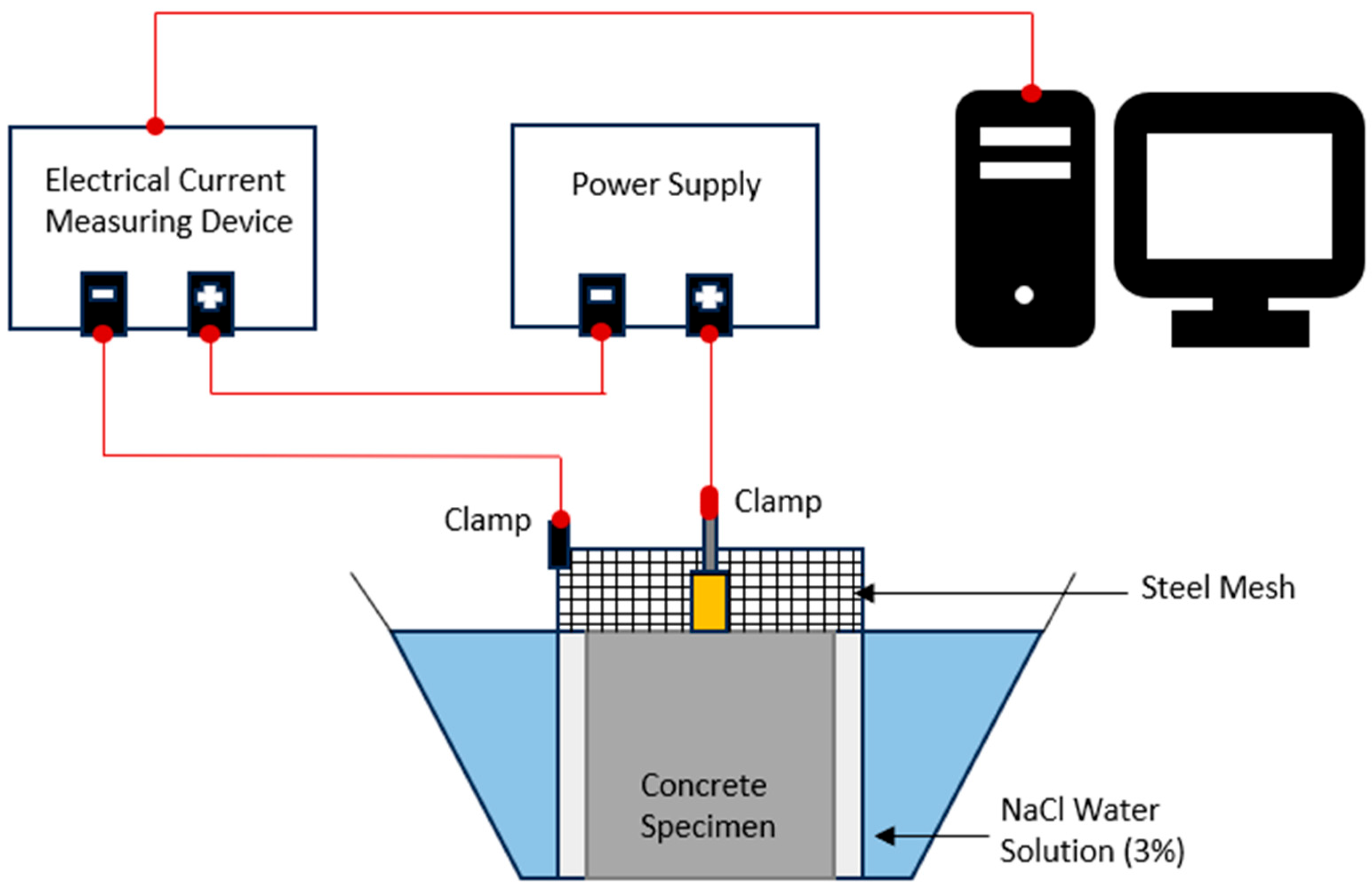
4.2. Development of Numerical Model

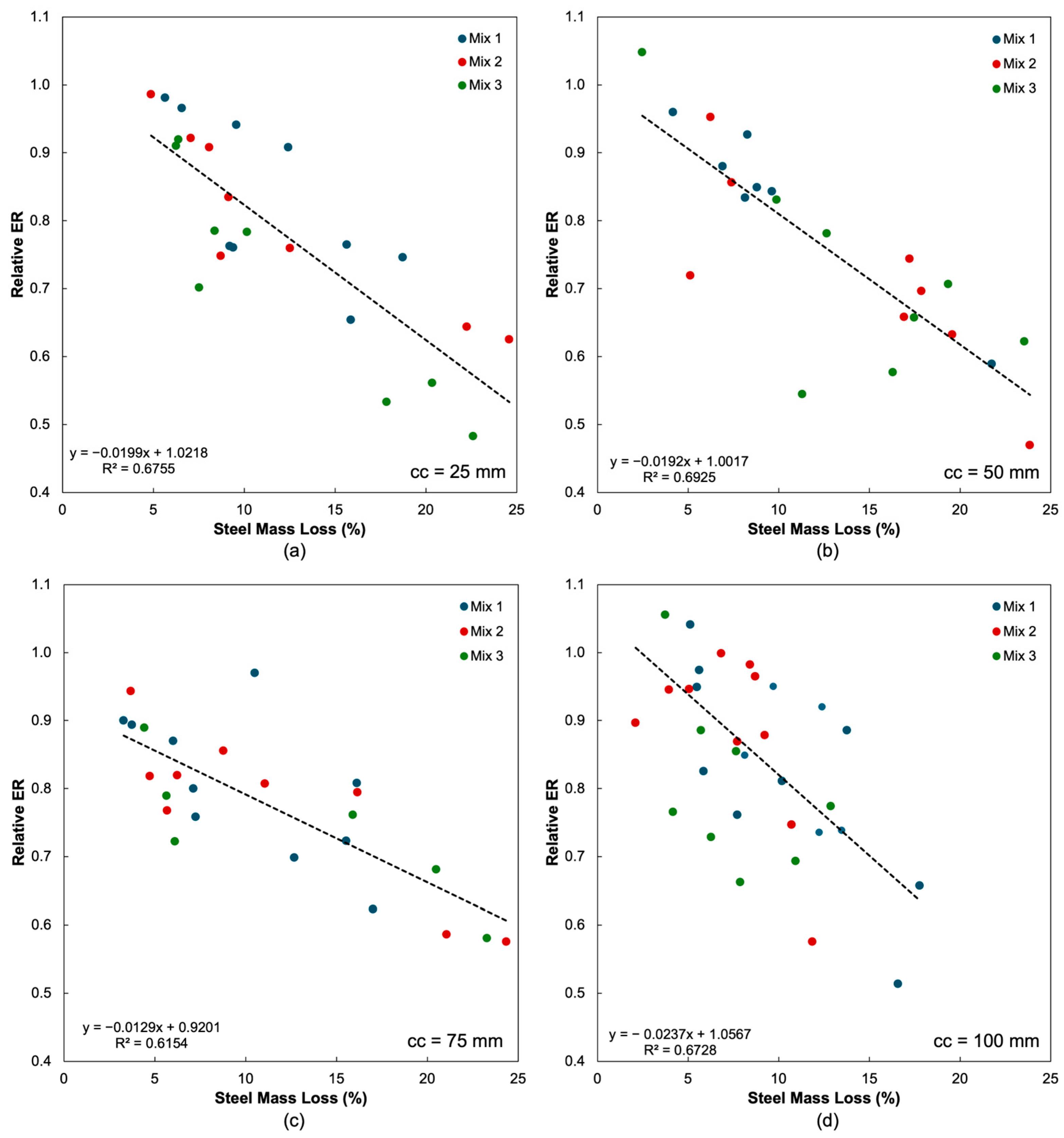
In the development of the numerical model, the electrical resistivity (ER) values used as input parameters were derived from the empirical relationships established in Figure 8. The linear equations derived from Figure 8 are incorporated into the numerical simulation strictly as boundary-condition inputs rather than as deterministic corrosion laws. Their role is to impose experimentally observed reductions in electrical resistivity (ER) associated with increasing steel mass loss under controlled and consistent test conditions. These relationships serve as first-order experimental constraints that calibrate the electrical conductivity field so that the simulated surface ER response matches laboratory measurements, while the predicted corrosion-affected zone is governed primarily by geometric configuration, conductivity contrasts, and subsequent nonlinear regression analysis. Therefore, the moderate goodness of fit of the linear trends does not undermine the reliability of the simulation outcomes. The final predictive framework does not rely on these equations to model corrosion kinetics, but instead uses them as effective representation of measured ER behavior, with associated uncertainties explicitly acknowledged and shown through sensitivity analyses to have limited influence on the overall conclusions.

These equations quantified the correlation between relative ER and steel mass loss at varying concrete cover depths, providing realistic boundary conditions for the simulation. By integrating these experimentally obtained relationships, the model ensured that the simulated electrical behavior of the reinforced concrete accurately reflected the physical effects of corrosion observed during testing. This approach enabled a more reliable calibration of the COMSOL Multiphysics model, bridging the experimental and computational components of the study and reinforcing the predictive capability of the simulation results.

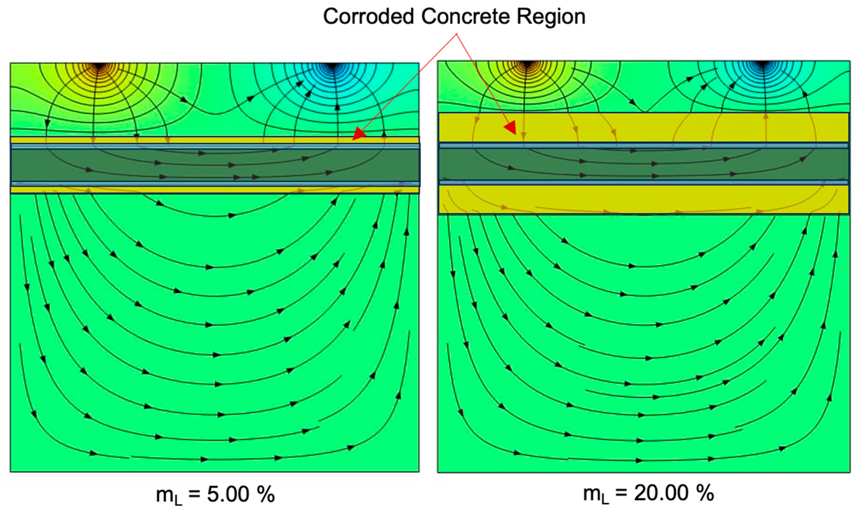
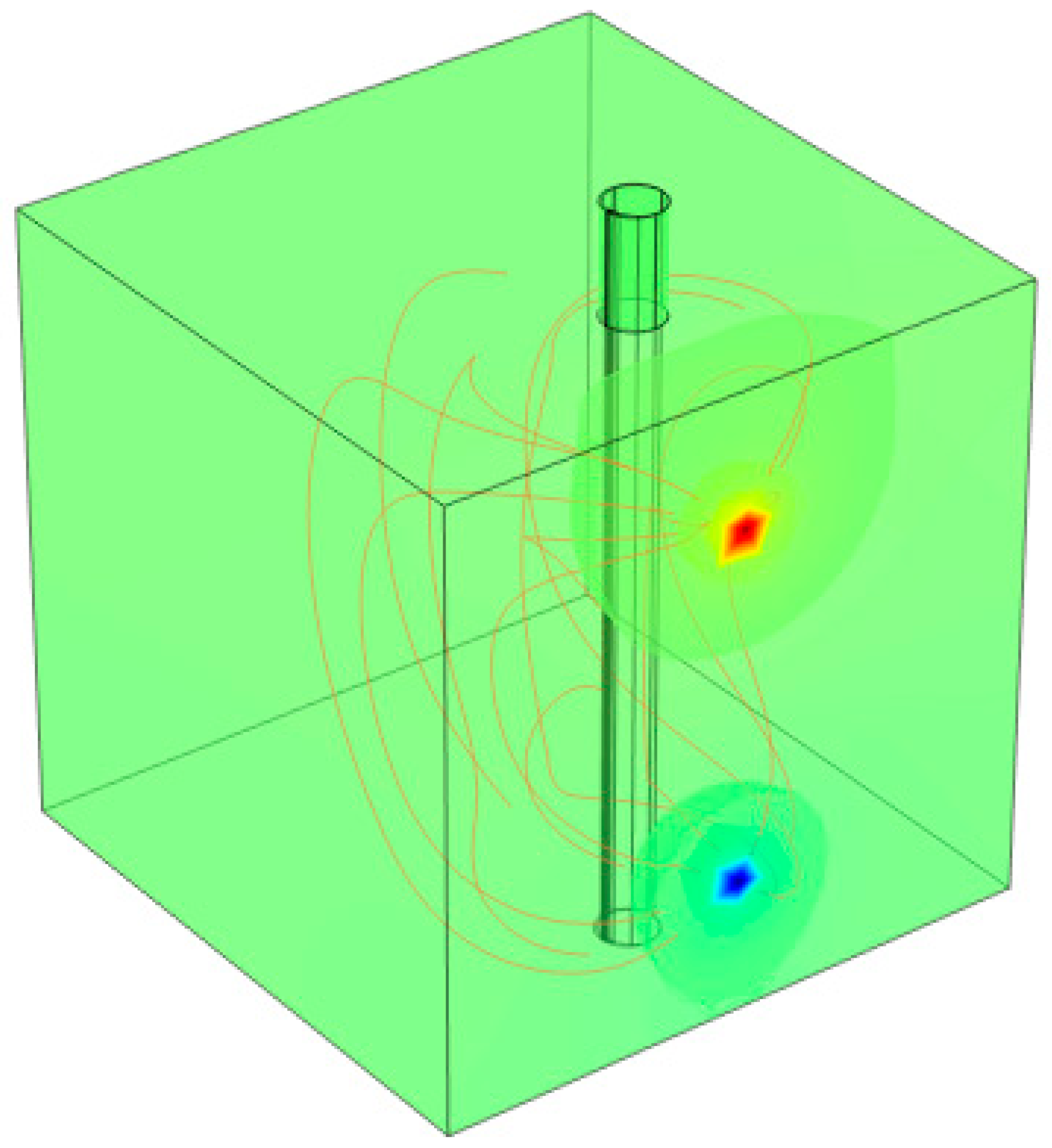
Figure 9 illustrates the electric potential distribution within reinforced concrete as influenced by different levels of steel mass loss and corresponding diameters of the corroded zone. It presents the potential field and current density streamlines around the rebar embedded in concrete, helping visualize how corrosion affects current flow patterns. A consistent trend is observed: as steel mass loss increases, the diameter of the corroded region expands, and the localized changes in electrical conductivity become more pronounced. These shifts in material properties alter the path and intensity of the electrical field, concentrating the equipotential lines and current streamlines around the deteriorated zones.

Notably, the simulations with 5% and 20% mass losses, highlighted in this study, show contrasting behaviors. At 5% loss, the potential gradient remains relatively uniform, and the electric field lines show smoother distributions, indicating minor disruption to the electrical conductivity of the concrete matrix. In contrast, the 20% mass loss case reveals significantly compressed and distorted equipotential lines around the enlarged corroded region, demonstrating intensified field concentration due to more extensive material degradation. This behavior underscores the influence of corrosion severity on signal distortion, which is crucial for interpreting non-destructive test data such as electrical resistivity. These findings validate the need to incorporate variable corrosion geometries in simulation-based assessments of reinforced concrete structures.

Table 2. Relative electrical resistivity (ER)—steel mass loss ($m_L)$ equation used for the simulation in this study.

cc (mm)	Relative ER Equation
25	${\mathsf{\alpha }}_{\mathsf{\rho }}=-0.0199 m_L+1.0218$
50	${\mathsf{\alpha }}_{\mathsf{\rho }}=-0.0192 m_L+1.0017$
75	${\mathsf{\alpha }}_{\mathsf{\rho }}=-0.0129 m_L+0.9201$
100	${\mathsf{\alpha }}_{\mathsf{\rho }}=-0.0237 m_L+1.0567$

presents the empirical equations that describe the relationship between relative electrical resistivity (ER) and steel mass loss at different concrete cover (cc) values. These equations were derived from regression analyses of experimental data, and their forms were guided by relationships established in related studies [91], which demonstrated that electrical resistivity decreases nonlinearly with increasing corrosion level. The fitted models reflect this inverse relationship, where ER diminishes progressively as steel mass loss increases, indicating enhanced ionic conductivity due to corrosion by-products and moisture ingress in the concrete matrix. 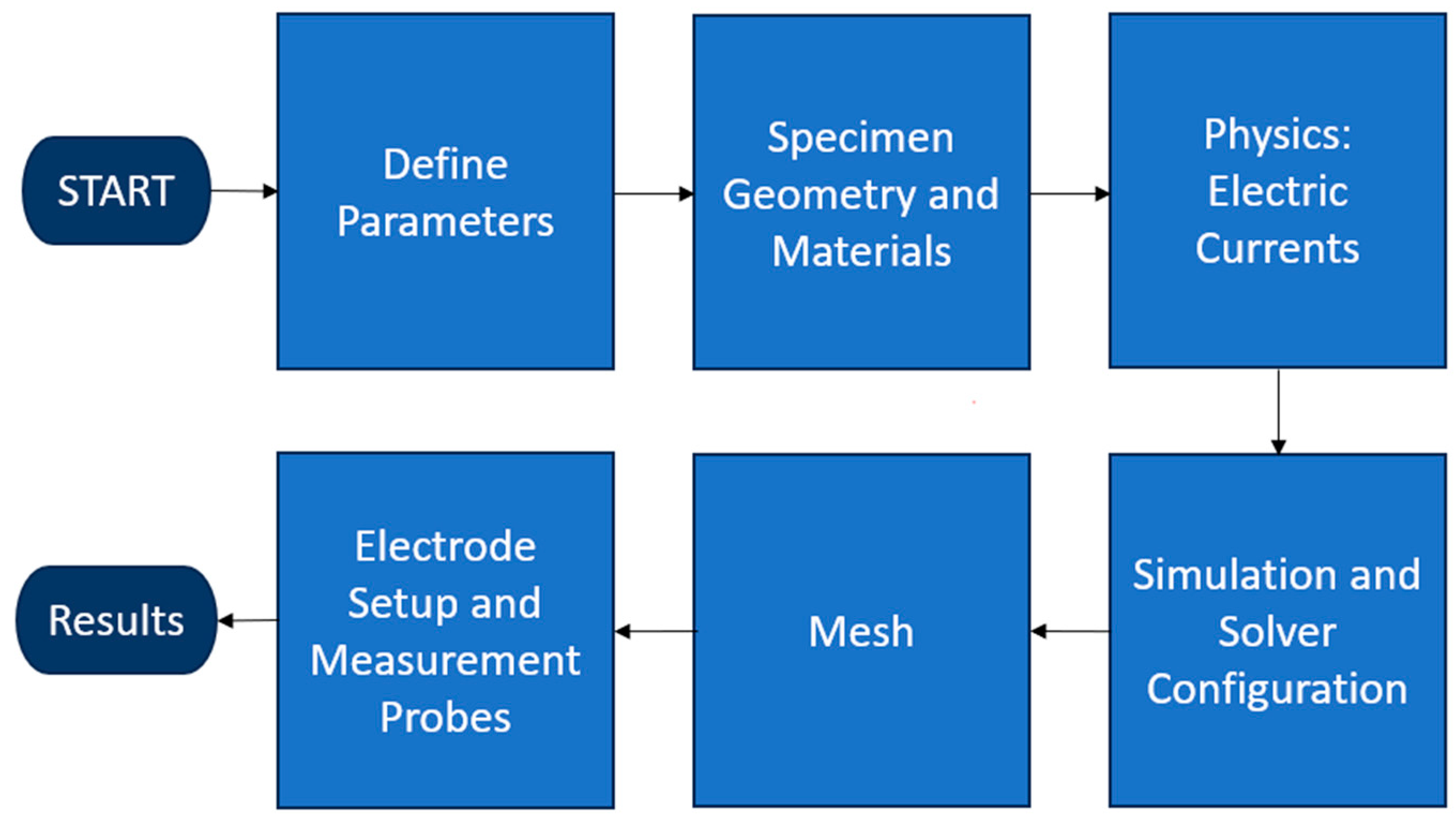The derived equations were subsequently used as input parameters in the numerical simulation (Section 3.2.) to ensure that the modeled resistivity field accurately represents the experimentally observed corrosion behavior. This integration of empirical and literature-based formulations provides a reliable foundation for simulating corrosion-induced electrical potential distribution in reinforced concrete. These simulations, developed using COMSOL Multiphysics v6.2, reflect the modeled expansion of conductive zones around corroded steel bars and were calibrated using physical parameters consistent with prior experimental studies [54].

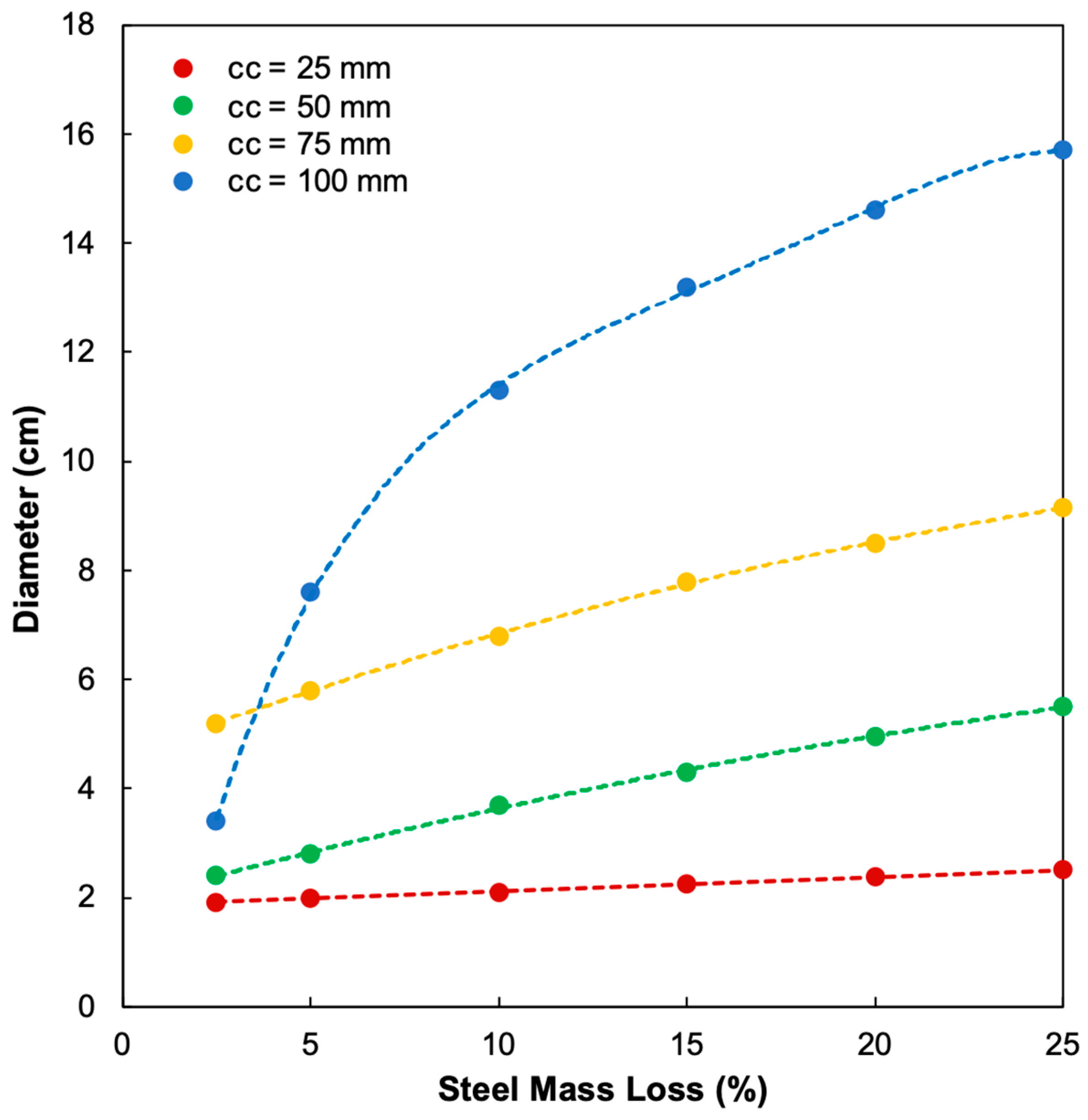
The simulation clearly demonstrates that as steel mass loss increases, the diameter of the corroded region in the concrete expands significantly. At 25 mm clear cover, diameters range from 1.92 cm at 2.5% mass loss to 2.52 cm at 25%. However, for specimens with 100 mm cover, this range expands dramatically from 3.4 cm to 15.7 cm over the same corrosion levels. These results emphasize that greater concrete cover permits more lateral dispersion of corrosion by-products, enhancing ionic mobility and electrical conductivity in the surrounding matrix [9,92].

This radial growth behavior of the corroded zone underlines the direct relationship between mass loss and apparent electrical resistivity (ER), where increased corrosion results in lower ER values due to elevated ionic content and moisture levels near the steel–concrete interface [52,66].

Across all cover depths, the expansion of corrosion diameters shows a non-linear progression. Between 10% and 20% steel mass loss, the rate of growth accelerates, especially for thicker concrete covers. This supports the electrochemical theory that corrosion expansion becomes more aggressive after the breakdown of the passive layer and accumulation of iron oxides [7,13]. The modeling outcomes corroborate the experimental trend where relative ER decreased sharply with increasing corrosion [74], indicating the widening extent of deterioration.

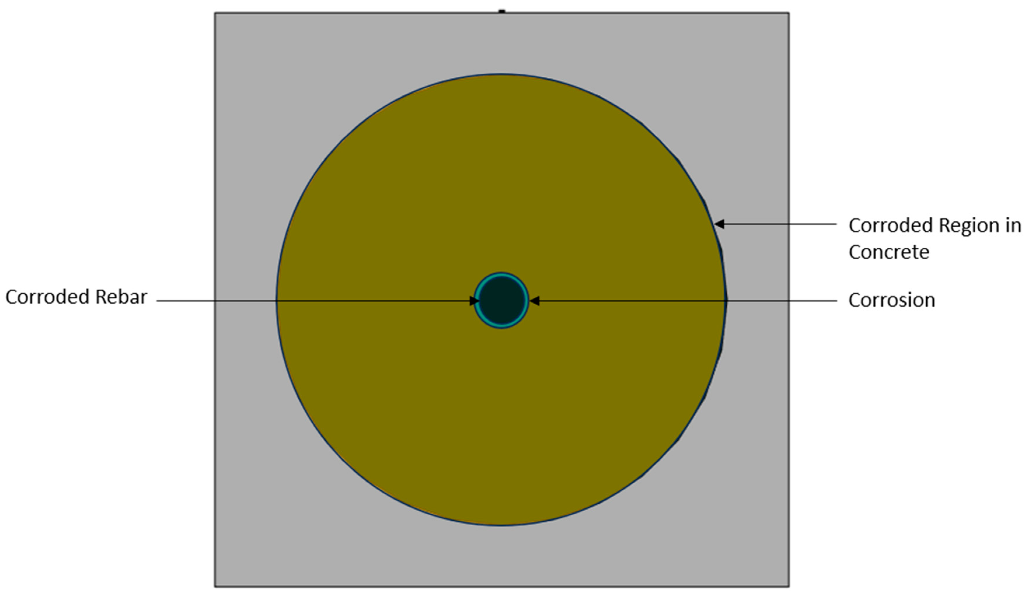
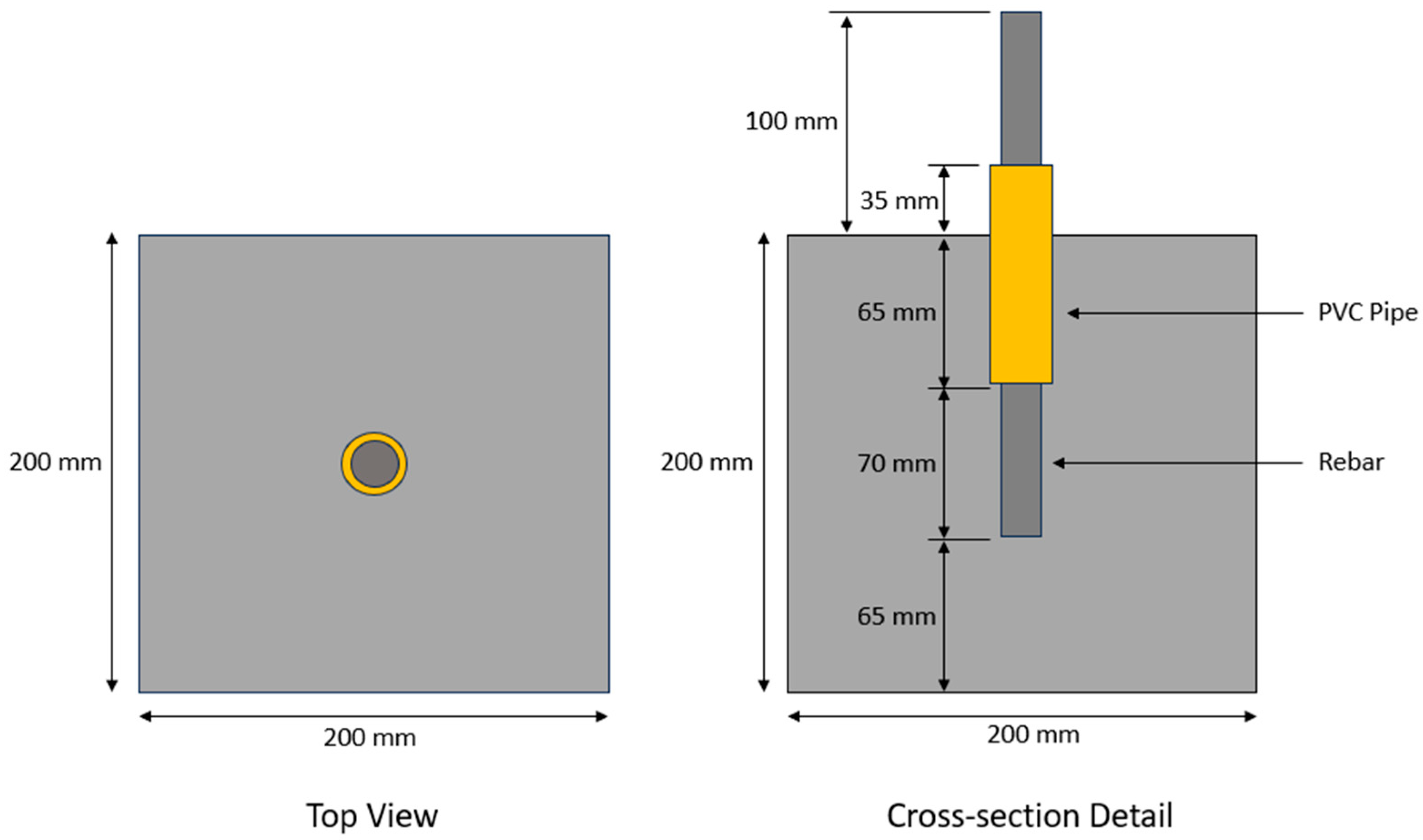
In this study, the term diameter refers to the diameter of the corrosion-affected region in the surrounding concrete matrix (Dc), as determined from numerical simulations and regression modeling, and not the diameter of the reinforcing steel bar (Db = 19 mm). The corrosion-affected diameter represents the spatial extent of concrete influenced by corrosion-induced changes in electrical conductivity and microstructural deterioration.

Figure 10 illustrates the relationship between steel mass loss and the corresponding diameter of the corrosion-affected region in the concrete (Dc) under varying concrete cover (cc) conditions. As shown, the diameter of the corrosion-affected region in the surrounding concrete increases with steel mass loss, reflecting the volumetric expansion of corrosion products surrounding the rebar. However, the extent of this increase is strongly influenced by the thickness of the concrete cover. Specimens with larger cover depths (75 mm and 100 mm) display a more pronounced growth in measured diameter compared with those having thinner covers (25 mm and 50 mm). This behavior indicates that a thicker concrete cover allows more lateral accommodation and propagation of corrosion-induced cracking, resulting in greater apparent surface expansion. The dashed trendline represents the linear regression model, which provides a reasonable but simplified fit to the data. Nevertheless, the increasing curvature of the plotted points, particularly for 75 mm and 100 mm cc, highlights a nonlinear relationship between steel mass loss and corrosion-induced diameter change, supporting the adoption of mathematical models for more accurate characterization of corrosion effects.

4.3. Statistical Analysis and Predictive Modelling

To evaluate the most suitable mathematical relationship between the diameter of the corroded region in the concrete and the independent variables, concrete cover (cc) and steel mass loss ($m_L$), several nonlinear regression models were developed and compared. The models tested include exponential, power, logarithmic, and third-degree polynomial forms. The quality of each model was assessed using the coefficient of determination ($R^2$) and the Root Mean Square Error (RMSE), which together provide insight into the explanatory power and predictive accuracy of each function.

The exponential model, used to predict the diameter of the corroded region based on steel mass loss and concrete cover, demonstrated a generally increasing trend but exhibited noticeable limitations in accuracy. While it captured the overall growth pattern of corrosion diameter with increasing mass loss, its predictions showed greater deviation from the simulation data, particularly at higher corrosion levels. This resulted in a lower coefficient of determination ($R^2$ = 0.923) and a higher RMSE compared to the third-degree polynomial model. The exponential model tended to overestimate the diameter in some cases, especially for specimens with thicker concrete cover, suggesting its limited capacity to reflect the complex, nonlinear nature of corrosion propagation. Although it offers a simplified mathematical representation, its predictive reliability is inferior to polynomial regression, making it less suitable for detailed diagnostic modeling.

As shown in Table 2 and

Table 3. Empirical equations for estimating corroded steel diameter based on concrete cover and steel mass loss.

Model	Equation
Exponential model	$D=e^{-0.1202+0.02054\left(cc\right)+0.03271\left(m_L\right)}$
Power model	$D={0.02713\times cc}^{1.0991}\times {m_L}^{0.3413}$
Logarithmic model	$D=-23.0763+6.0358\ln \left(cc\right)+2.1508\mathrm{l}\mathrm{n}\left(m_L\right)$
Linear model	$D=0.05921\left(cc\right)+0.10581\left(m_L\right)-2.02877$
Third-degree polynomial model	$D=2.3277-0.068088\left(cc\right)+0.016289\left(m_L\right)+0.001699\left({cc}^2\right)$$+0.003624\left(cc\times m_L\right)-0.008223\left({m_L}^2\right)-0.000011\left({cc}^3\right)$$+0.000087\left({cc}^2\times m_L\right)-0.000317\left(cc\times {m_L}^2\right)+0.000492\left({m_L}^3\right)$

, the power model yielded an $R^2$ value of 0.912 with an RMSE of 1.206, slightly lower than the exponential model. This form implies that the diameter changes as a multiplicative power function of both parameters. The exponents greater than zero confirm that both cc and $m_L$ positively influence the resulting diameter values. Despite the relatively high $R^2$, the model tends to underestimate extreme values, suggesting that its scaling behavior may not align with the more complex physical interactions occurring during corrosion.

The logarithmic model provided an $R^2$ value of 0.776 and an RMSE of 1.929, which is substantially lower than those of the exponential and power models. While this relationship captures some degree of correlation, it performs poorly for large values of cc and $m_L$, where nonlinearity is more pronounced. This model therefore lacks sufficient predictive capability and should be considered unsuitable for representing the dataset.

The linear regression model established a direct relationship between rebar diameter, concrete cover (cc), and steel mass loss ($m_L$) using a first-order equation. The model achieved an $R^2$ value of 0.831 and an RMSE of 1.67, indicating that it explains approximately 83.1% of the variation in the observed data. While this reflects a reasonably strong correlation, the relatively high prediction error suggests that the linear model cannot fully capture the curvature and complex interaction effects between the independent variables. In practical terms, this means that the change in diameter due to corrosion does not increase uniformly with cc and $m_L$, but rather follows a nonlinear trend that the linear model oversimplifies. Therefore, although the linear regression provides a basic approximation and can serve as an initial benchmark, it is less suitable for precise predictive analysis compared to higher-order nonlinear models such as the polynomial regression, which demonstrated superior accuracy and a closer representation of the experimental behavior.

The third-degree polynomial model achieved the highest $R^2$ value of 0.984 and an RMSE of 0.513, indicating an excellent fit between experimental and predicted data. The inclusion of squared and cubic interaction terms allows this model to capture the curvature and interaction effects that simpler functional forms cannot represent. This superior performance demonstrates that the relationship between the diameter of corroded region in the concrete, concrete cover, and steel mass loss is highly nonlinear and best described by a multivariate polynomial function.

The comparison clearly shows that the third-degree polynomial model provides the most accurate and flexible representation of the relationship between cc, $m_L$, and the diameter of the corroded region in the concrete. Its high $R^2$ value and low RMSE confirm that the relationship between rebar diameter, concrete cover, and steel mass loss is highly nonlinear. While the exponential and power models provide reasonably good approximations and may have clearer physical interpretations, they fail to capture the interaction effects between the two independent variables. The polynomial model, on the other hand, accurately reflects these interdependencies and should therefore be used as the primary regression equation for predictive analysis and structural assessment in this study.

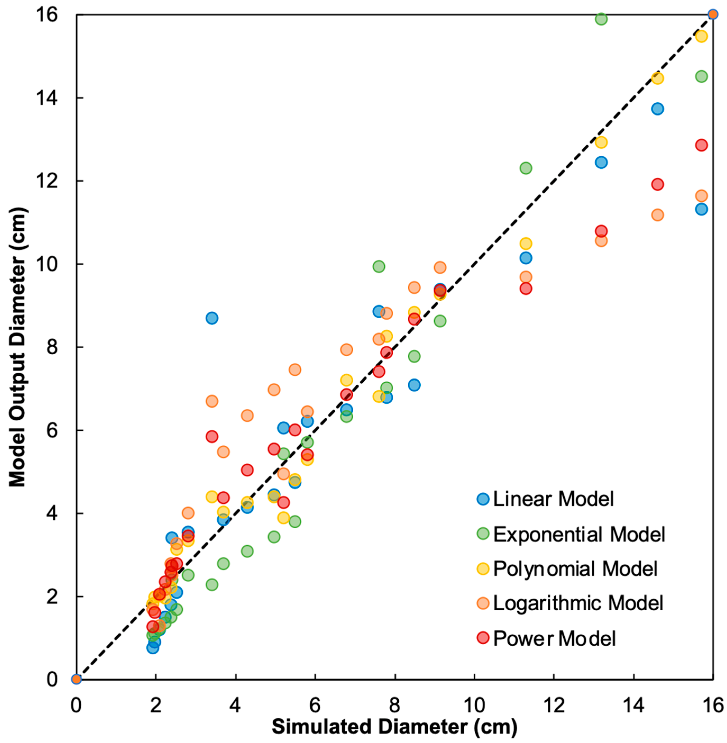
To further validate the accuracy of the nonlinear regression models that were developed and compared, Figure 11 compares the predicted outputs of the models with the simulation results derived from COMSOL Multiphysics.

Based on the five plots comparing the simulation results with different predictive models (third-degree polynomial, exponential, power, logarithmic, and linear), we can assess the accuracy and fitting performance of each model in estimating the diameter of the corroded region. The third-degree polynomial model shows a strong agreement with the simulation values, with points closely following the diagonal line, indicating both accuracy and consistency. This supports the earlier finding in the paper (see

Table 4. Statistical performance of the empirical models in predicting corroded steel diameter.

Model	${\mathit{R}}^2$	RMSE
Exponential model	0.923	1.131
Power model	0.912	1.206
Logarithmic model	0.776	1.929
Linear model	0.831	1.67
Third-degree polynomial model	0.984	0.513

) where this model achieved the highest coefficient of determination ($R^2$ = 0.984) and the lowest RMSE (0.513), confirming its robustness in capturing the nonlinear behavior influenced by steel mass loss and concrete cover. The inclusion of squared and interaction terms allowed the model to accommodate the highly non-linear relationship between cover thickness, steel degradation, and corroded region diameter [74].

In contrast, the exponential, power, logarithmic, and linear models exhibit significantly more deviation from this simulation results. The exponential and power models, while showing a general trend, demonstrate considerable scatter, especially for higher values. This is reflected in their lower $R^2$ values (0.923 and 0.912, respectively) and higher RMSE values compared to the polynomial model. The logarithmic model performed the poorest, displaying large deviations, particularly at both low and high ranges, and producing even negative predictions in some cases, indicating its limited applicability in this context.

These comparisons underscore the importance of selecting an appropriate model that can capture the complex interaction between parameters affecting the diameter of corrosion-induced damage. The third-degree polynomial model is recommended as the most reliable option for future applications due to its superior predictive capability.

However, the experimental dataset used for model calibration was limited in scope, particularly in terms of specimen geometry, corrosion levels, and material variability. As such, while the mathematical approach provides valuable insight into corrosion behavior and resistivity response, it is not sufficient on its own to fully explain the complex phenomena occurring in reinforced concrete. Future research should integrate multi-parameter experimental data, variable material properties, and advanced electrochemical models to improved realism and broaden the applicability of the predictive framework.

The simulation part offers critical insights into the practical interpretation of surface ER measurements. For instance, concrete elements with thinner covers show limited corrosion spread and hence smaller reductions in ER, potentially leading to underestimation of corrosion severity if the influence of cover depth is neglected [79,81]. On the other hand, thicker covers show greater apparent diameters and more significant ER drops due to higher diffusivity and moisture retention.

4.4. Practical Applications and Guidelines

The experimental results demonstrated a strong inverse correlation between electrical resistivity (ER) and steel mass loss in reinforced concrete specimens exposed to a corrosive environment. As corrosion increased, ER values decreased due to higher ionic conductivity at the steel–concrete interface. Specifically, the relative ER dropped from approximately 1 to 0.52 as steel mass loss rose from 0% to 8%, with a Pearson correlation coefficient of r = −0.714. However, variability in results suggests that external factors such as concrete cover thickness and electrode spacing also influence ER measurements and must be accounted for in real-world diagnostics.

The obtained results are consistent with values reported in the literature for electrical resistivity-based corrosion assessment. Concrete resistivity values below 10 kΩ·cm are typically associated with a high probability of active corrosion, while values above 20 kΩ·cm indicate low corrosion risk [13]. A decrease in resistivity from approximately 15 kΩ·cm to below 5 kΩ·cm with increasing corrosion activity under chloride exposure was observed [14]. Also, strong correlations between resistivity and corrosion current density (R² > 0.80) in chloride-contaminated reinforced concrete specimens was identified. Similarly, it was demonstrated that decreasing resistivity corresponds to increasing ionic transport and corrosion kinetics [9,53]. The relative ER reductions and correlation coefficients obtained in the present study fall within the ranges reported in these studies, supporting the validity of the proposed experimental-numerical framework. However, unlike previous studies that primarily focused on corrosion probability or corrosion rate, the present model extends the application of ER to predict the spatial extent of corrosion-affected regions in concrete.

Regarding corrosion-induced damage extent, corrosion penetration and cracking zones ranging from several millimeters to centimeters depending on cover depth and corrosion level were determined, which are comparable to the corrosion-affected diameters predicted in this study (2–15 cm for cover depths of 25–100 mm) [23,61]. This agreement further confirms that the predicted corrosion-affected region sizes are physically realistic and consistent with reported experimental observations.

Table 5. Computed diameters of the corroded region in concrete for varying relative electrical resistivity ranges and concrete cover values.

cc (mm)	Diameter of Corroded Region Based on Relative ER Range
	0.5–0.6	0.6–0.7	0.7–0.8	0.8–0.9	>0.9
25	2.52	2.37	2.24	2.10	1.92
50	5.50	4.96	4.30	3.70	2.40
75	9.14	8.50	6.80	5.80	5.20
100	14.61	13.20	11.30	7.60	3.40

presents the computed diameter of the corroded region in concrete as a function of both relative electrical resistivity (ER) and concrete cover (cc) thickness. The results clearly demonstrate an inverse relationship between ER and extent of corrosion, where lower resistivity values (0.5–0.6) correspond to larger corroded diameters, indicating more severe corrosion activity. Conversely, as the relative ER approaches values greater than 0.9, the corresponding diameters decrease significantly, signifying a less corroded condition. These observations are consistent with previous studies showing that thicker concrete cover leads to increased corrosion propagation when combined with reduced electrical resistivity values [93,94].

Furthermore, the data show that specimens with thicker concrete covers exhibit substantially larger corroded diameters at equivalent ER ranges. For instance, at an ER range of 0.5–0.6, the corroded region diameter increased from 2.52 cm for 25 mm cc to 14.61 cm for 100 mm cc. This observation implies that greater concrete cover allows the corrosion products to expand and propagate laterally within the concrete matrix, producing a more extensive corroded zone. The same pattern is evident across all ER ranges, reinforcing that both cover thickness and ER values are key influencing factors in determining the spatial extent of corrosion-induced damage.

To model the corroded region diameter based on corrosion level and concrete cover depth, several regression models were evaluated. Among these, the third-degree polynomial model provided the best fit, with an $R^2$ of 0.984 and RMSE = 0.513, outperforming exponential and power models. This model effectively captured the nonlinear relationship and interaction between parameters. Validation against COMSOL Multiphysics simulations showed excellent agreement, supporting its reliability as a predictive tool.

COMSOL-based simulations illustrated how corrosion-affected zones expand radially with increasing steel mass loss, especially in specimens with thicker concrete cover. For instance, at 25% mass loss, the corroded diameter expanded from 2.52 cm (25 mm cover) to 15.7 cm (100 mm cover). This underscores the significant influence of concrete cover on corrosion propagation and supports earlier findings that thicker covers enable more extensive lateral corrosion spread and conductivity changes. The simulations validated that polynomial model from Section 4.2 and reinforced the utility of ER as a diagnostic tool when properly calibrated for geometric factors.

While the findings across Section 4.1, Section 4.2, Section 4.3 demonstrate a coherent relationship between corrosion, electrical resistivity, and concrete geometry, validated by both experimental and numerical models, certain modeling assumptions introduce limitations that should be addressed. Based on a fully corroded specimen, all simulations used a constant electrical conductivity value ($\sigma$) of 0.2 S/m for the corroded region in the concrete, which may not fully reflect field variability due to moisture gradients, temperature, or crack development. This simplification could affect prediction accuracy in highly heterogenous environments.

Moreover, the results presented in this study are derived from a limited experimental dataset, which may restrict the generalizability and precision of the computed values. To enhance the accuracy and robustness of future research, it is recommended that additional datasets be incorporated to capture a wider range of parameters and corrosion conditions. The numerical simulations in this study were performed using a cubic reinforced concrete specimen geometry to ensure consistency with the experimental program, and to allow systematic parametric investigation. However, practical reinforced concrete structures typically exhibit more complex geometries, including slabs, beams, columns, and large-scale structural members with non-uniform boundary conditions. Future studies should extend the developed numerical framework to alternative geometrical configurations to investigate geometric scaling effects, three-dimensional current flow behavior, and field applicability of ER-based corrosion assessment models. Such extensions will improve the robustness and generalizability of the proposed predictive framework. Lastly, since the current simulation focuses on a single-diameter analysis, it is advisable that subsequent research consider multi-layer or volumetric simulations to depict partial or non-uniform corrosion development within reinforced concrete structures more accurately.

Building upon the validated modeling framework and the observed relationship between steel mass loss and the corrosion-affected diameter, it is also important to evaluate how sensitive the simulation outputs are to the assumed material properties, particularly the electrical conductivity ($\sigma$) of the corroded region in the concrete. Since $\sigma$ plays a crucial role in defining the distribution of current flow during resistivity measurements, even small changes in this parameter may affect the predicted extent of corrosion. The following analysis presents the results of simulations conducted using a fixed concrete cover of 50 mm while varying $\sigma$ values across a realistic range were applied, as summarized in

Table 6. Effect of Varying Electrical Conductivity ($\sigma$) on Simulated Corrosion-Affected Zone Diameter.

$\mathit{\sigma }$	$\mathbf{D} (2.5\% {\mathit{m}}_{\mathit{L}}$)	$\mathbf{D} (5\% {\mathit{m}}_{\mathit{L}}$)	$\mathbf{D} (10\% {\mathit{m}}_{\mathit{L}}$)	$\mathbf{D} (15\% {\mathit{m}}_{\mathit{L}}$)	$\mathbf{D} (20\% {\mathit{m}}_{\mathit{L}}$)	$\mathbf{D} (25\% {\mathit{m}}_{\mathit{L}}$)
0.1 S/m	2.42 cm	2.9 cm	3.84 cm	4.5 cm	5.16 cm	5.74 cm
0.2 S/m (Assigned)	2.4 cm	2.8 cm	3.7 cm	4.3 cm	4.96 cm	5.5 cm
0.5 S/m	2.38 cm	2.8 cm	3.62 cm	4.22 cm	4.84 cm	5.38 cm
0.75 S/m	2.36 cm	2.78 cm	3.6 cm	4.2 cm	4.82 cm	5.36 cm

.

Table 6 presents the effect of varying electrical conductivity ($\sigma$) values assigned to the corroded region in the concrete on the predicted corrosion-affected zone diameters, using a constant concrete cover of 50 mm across all simulations. The steel mass loss levels ranged from 2.5% to 25%, while $\sigma$ was varied from 0.1 S/m to 0.75 S/m to assess its influence on the apparent corrosion diameter.

The results show a consistent trend: as $\sigma$ increases, the predicted corrosion diameter slightly decreases. For instance, at 20% steel mass loss, the predicted diameter decreases from 5.16 cm ($\sigma$ = 0.1 S/m) to 4.82 cm ($\sigma$ = 0.75 S/m), indicating a modest but measurable sensitivity to electrical conductivity. This effect can be attributed to the fact that higher $\sigma$ values reduce electrical resistivity in the corroded zone, leading to more concentrated current flow and a tighter estimation of the current field boundary during simulation.

Despite this, the overall sensitivity of the model to changes in $\sigma$ remains relatively low. Across all mass loss levels, the change in predicted diameter with increasing $\sigma$ is generally under 10%. This suggests that, while $\sigma$ influences the results, the concrete geometry, particularly the cover depth of 50 mm, plays a more dominant role in defining the dispersion of current and thus the apparent boundary of the corrosion-affected region.

The base conductivity used in the main simulation results, $\sigma$ = 0.2 S/m, lies within the typical range reported for chloride-contaminated or cracked concrete [74,77]. However, this table highlights the importance of careful calibration: real-world concrete may have varying conductivity depending on moisture content, temperature, and the presence of cracks, which are not captured in a constant-$\sigma$ model.

From a practical standpoint, this sensitivity analysis reinforces the need to: (1) validate $\sigma$ values against field or lab measurements; (2) treat $\sigma$ as a variable during calibration in heterogenous environments; and (3) consider dynamic modeling of conductivity when moisture gradients or cracks are known to exist. Although the changes observed in Table 6 are moderate, their cumulative effect in large-scale assessments or service life predictions could be significant. Thus, incorporating $\sigma$ variation into future modeling frameworks is essential to improve the reliability and realism of corrosion simulations under diverse exposure conditions.

While the influence of concrete conductivity on the simulated corrosion response is essential to understand material behavior, another equally important parameter is the electrode spacing used in surface resistivity measurements. Electrode spacing determines the depth and spread of current flow within the concrete, and thus directly affects the sensitivity and accuracy of the corrosion assessment. To further investigate this, an additional simulation was conducted using a wider electrode spacing while keeping the concrete cover constant at 50 mm. The results are presented and discussed in

Table 7. Effect of Electrode Spacing on Predicted Corrosion-Affected Zone Diameter.

Electrode Spacing	$\mathbf{D} (2.5\% {\mathit{m}}_{\mathit{L}}$)	$\mathbf{D} (5\% {\mathit{m}}_{\mathit{L}}$)	$\mathbf{D} (10\% {\mathit{m}}_{\mathit{L}}$)	$\mathbf{D} (15\% {\mathit{m}}_{\mathit{L}}$)	$\mathbf{D} (20\% {\mathit{m}}_{\mathit{L}}$)	$\mathbf{D} (25\% {\mathit{m}}_{\mathit{L}}$)
38 mm (Assigned)	2.4 cm	2.8 cm	3.7 cm	4.3 cm	4.96 cm	5.5 cm
50 mm	2.18 cm	2.46 cm	3 cm	3.5 cm	4.04 cm	4.5 cm

.

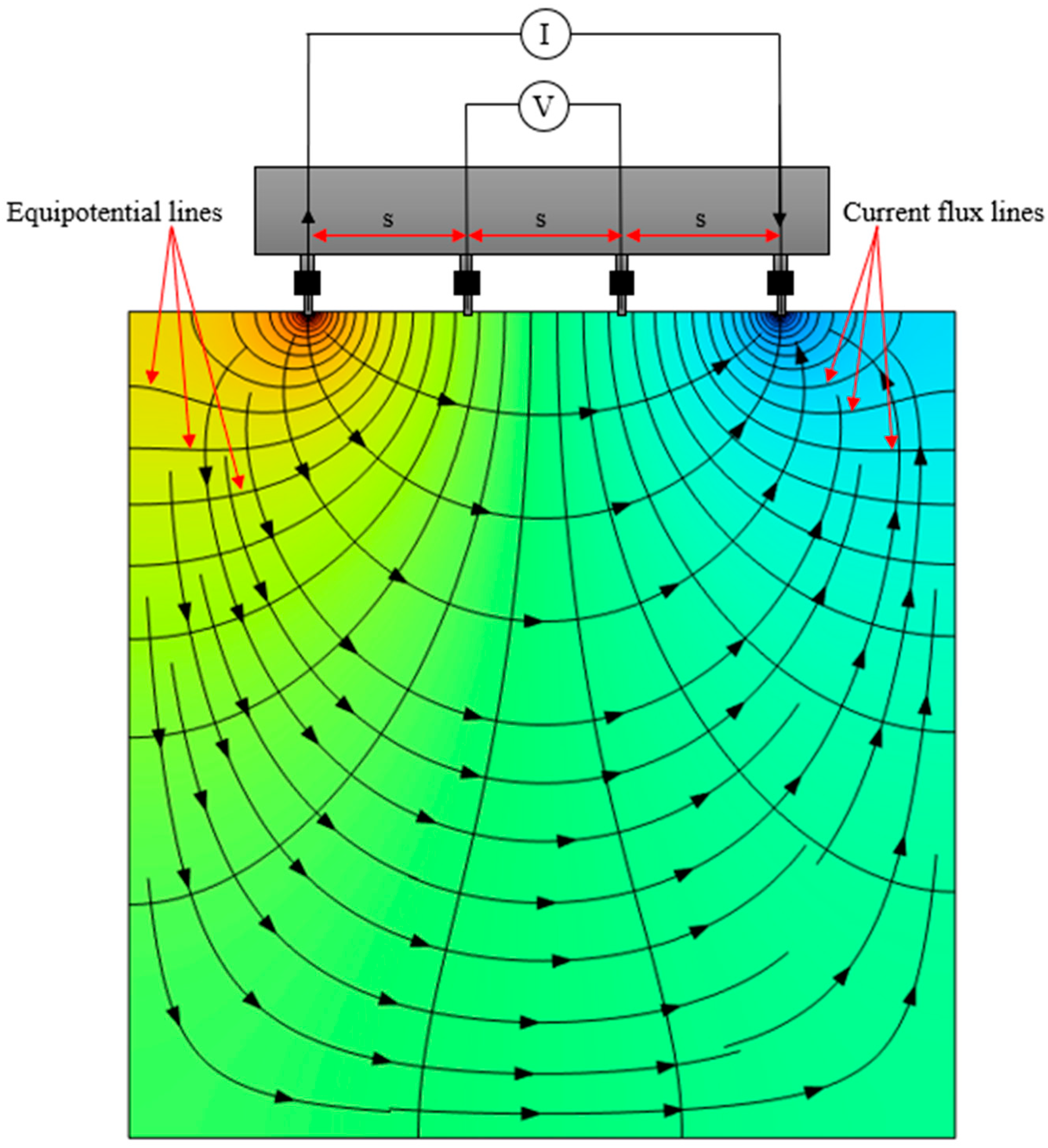
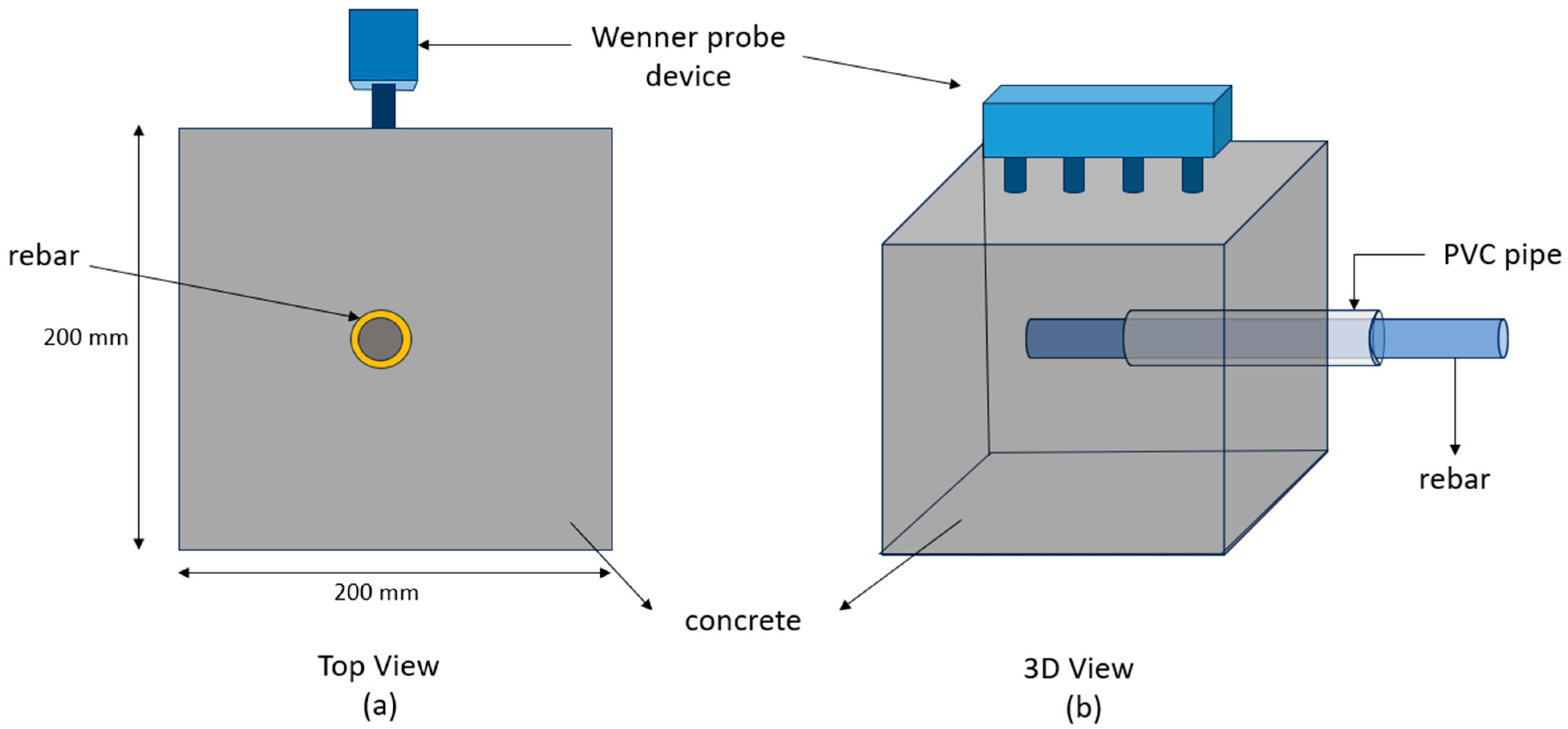
Table 7 examines how changes in electrode spacing influence the simulation results for the corrosion-affected zone diameter under a fixed concrete cover of 50 mm. The analysis was conducted by comparing two common four-probe spacings: the assigned 38 mm used in the base simulation and a wider spacing of 50 mm. These two electrode spacings were evaluated because these dimensions correspond to commercially available Wenner probe configurations, making them practical and widely adopted in both laboratory and field measurements. The simulations were carried out for steel mass loss values ranging from 2.5% to 25%.

The results indicate that when the electrode spacing was increased from 38 mm (assigned) to 50 mm, the simulated diameters slightly decreased across all corrosion levels. This suggests that, for the specimen and geometry used (50 mm cover), the 38 mm spacing was more sensitive to the localized resistivity change around the corroded rebar, while the wider 50 mm spacing sampled a larger concrete volume and therefore produced a more averaged, and slightly smaller, apparent corrosion diameter.

The influence of electrode spacing on the simulation outcome aligns with findings from field studies and existing literature, where greater probe spacing is associated with deeper current paths and lower overall resistivity readings [83]. However, it also introduces greater averaging over the concrete volume, which may slightly obscure the localized effects of corrosion, particularly at early stages.

From a practical standpoint, this result reinforces the need to standardize electrode spacing in both experimental and simulation protocols. Variation in spacing can introduce inconsistencies when comparing ER measurements across different setups or when calibrating models for field use. Additionally, the findings suggest that spacing should be selected based on the expected corrosion depth and the concrete cover, to balance resolution and sensitivity.

Given that the concrete cover remained constant at 50 mm, the observed differences can be attributed solely to changes in electrode spacing, highlighting its direct effect on measurement interpretation. This insight is critical for engineers and inspectors who rely on surface resistivity as a proxy for internal corrosion damage, especially in field applications where probe configurations may vary.

To enhance the accuracy and applicability of resistivity-based corrosion assessment models, it is strongly recommended that future numerical simulations integrate a broader range of variable parameters. Specifically, electrical conductivity ($\sigma$) should be treated as a dynamic property influenced by local moisture content, chloride concentration, and temperature gradients, rather than as a fixed value. Additionally, bar diameter ($d_b$) should be incorporated as a variable, as it directly affects the surface area exposed to corrosion and the resulting current density distribution. The inclusion of realistic crack scenarios, both in terms of geometry and conductivity, would significantly improve the representativeness of the models, as crack alter both ionic transport and current flow paths. Lastly, electrode spacing (s) should be parameterized across multiple values to capture its impact on measurement depth and resolution. Integrating these variables into a comprehensive, multi-parameter simulation framework will yield more robust, field-applicable models that can better inform inspection strategies, service life predictions, and rehabilitation planning for reinforced concrete structures.

While the present study establishes a calibrated relationship between electrical resistivity (ER) and measured steel mass loss under controlled exposure conditions, several limitations must be acknowledged. Electrical resistivity in reinforced concrete is influenced not only by corrosion progression but also by chloride ingress, moisture content, and saturation state. In this investigation, all specimens were measured under identical saturation conditions immediately after removal from the NaCl solution, and the analysis relied on relative ER normalized to uncorroded baseline values to reduce variability associated with mix composition and moisture differences. However, a dedicated control program isolating the effect of chloride ingress without corrosion was not performed. As a result, the correlation developed in this study reflects the combined influence of chloride contamination and corrosion under the tested protocol rather than a fully separated chloride-only effect. Future studies should include controlled chloride-ingress experiments to quantify its independent contribution to ER variation.

Additionally, the numerical simulation represents corrosion using an equivalent geometric reduction in steel cross-section and an effective high-conductivity corrosion zone surrounding the reinforcement. This approach enables tractable parametric analysis and calibration with experimental trends but does not explicitly model micro-scale pitting morphology, evolving anodic surface area, or localized corrosion heterogeneity. The simulation should therefore be interpreted as an effective field-scale approximation consistent with measured ER behavior rather than a detailed electrochemical pitting model. Incorporating nonuniform corrosion geometries and spatially variable conductivity fields in future simulations would improve realism and extend the applicability of the predictive framework.

Lastly, it is important to note that while the present study was conducted under controlled laboratory conditions, field measurements of electrical resistivity may be influenced by additional factors not fully represented in the experimental setup. In real structures, heterogenous moisture distribution, chloride gradients, cracking, temperature variation, and geometric complexity can significantly alter the measured ER response. These may introduce variability beyond that captured in the current model. Therefore, this study should be applied in field assessments with appropriate consideration of site-specific conditions, and future work should focus on validating the model under realistic structural environments.

5. Conclusions

This study investigated the application of electrical resistivity (ER) measurements in assessing steel corrosion in determining corrosion-affected zones in reinforced concrete, combining experimental testing with numerical simulation using COMSOL Multiphysics v6.2. Reinforced concrete cubes with controlled steel mass loss were evaluated using a four-probe Wenner configuration, and the corresponding changes in ER were analyzed in relation to corrosion progression and concrete geometry. The key findings are summarized as follows:

• A strong inverse relationship between electrical resistivity (ER) and steel mass loss in reinforced concrete was confirmed. As corrosion increased, ER values declined due to improved ionic conduction around the corroded rebar, validating ER as a viable non-destructive indicator of corrosion progression.
• A third-degree polynomial model was developed to estimate the diameter of the corrosion-affected zone based on steel mass loss and concrete cover. The model showed excellent accuracy ($R^2$= 0.984) and captured the nonlinear interaction between geometric and material parameters. Validation through simulation confirmed its reliability.
• Numerical simulations using COMSOL supported the experimental trends, showing that corrosion-affected zones expand with increasing steel loss and concrete cover. The results demonstrated how geometric factors influence current flow and support the use of ER-based diagnostics when modeled appropriately.
• Parametric analysis revealed that the model is only moderately sensitive to changes in electrical conductivity ($\sigma$), but more sensitive to electrode spacing. Wider spacing increased the predicted corrosion zone slightly, highlighting the need to standardize probe configurations for consistent assessment.
• The findings emphasize the importance of integrating variable parameters, such as $\sigma$, bar diameter, cracks, and electrode spacing, into future models. Doing so will improve the accuracy, adaptability, and practical relevance of ER-based corrosion assessment tools in structural monitoring.