1. Introduction
When a shield machine advances through small-radius curved sections, the interaction between the machine and the surrounding soil intensifies substantially [
1]. Under these conditions, the machine becomes prone to snakelike motion, a phenomenon that can cause segment dislocation, segment damage, and ground settlement from excessive ground loss [
2]. Conventional attitude control relies primarily on operator experience and judgment, yet the extreme alignment geometry of small-radius curves makes it difficult to achieve timely and optimal correction decisions through manual operation alone. There is consequently an urgent need for intelligent methods capable of accurately predicting shield machine attitude, to ensure both construction safety and quality under such demanding conditions.
Early research approached this problem from a theoretical mechanics perspective, establishing a fairly comprehensive kinematic model of shield tunneling. These foundational studies systematically analyzed how advance parameters influence curved-path motion [
3] and validated the resulting model through field observations in soft soil formations [
4]. As data acquisition capabilities subsequently improved, data-driven methods began to attract considerable attention. Random Forest was among the first techniques applied to real-time analysis and steering control of earth-pressure-balance shield attitudes [
5]. Shortly thereafter, a Bayesian-optimized LightGBM model outperformed conventional regression methods in simultaneously predicting multiple key tunneling parameters [
6]. Despite these advances, such methods remain constrained by their reliance on manual feature engineering and shallow mapping structures. Their capacity to capture the nonlinear dynamic coupling between tunneling parameters and attitude responses (coupling embedded in high-dimensional time-series signals) is therefore limited.
The rise of deep learning has progressively established sequence modeling as the mainstream approach for shield machine attitude prediction. Wavelet-transform-enhanced hybrid CNN-LSTM architectures were among the earliest deep models introduced for dynamic attitude and position prediction, and they convincingly demonstrated the advantage of sequence-based modeling [
7]. GRU-based deep networks subsequently enabled real-time prediction of shield movement trajectories with good generalization across multiple projects [
8], while hybrid models incorporating dual attention mechanisms over both time steps and feature dimensions yielded further accuracy gains [
9]. Novel hybrid deep learning architectures have also been explored for sustainable shield attitude prediction [
10]. Building on this foundation, researchers have extended the field in several productive directions: online multi-objective optimization [
11], physics-data-driven parallel multi-objective attitude control [
12], LSTM-Transformer long-range hybrid architectures [
13], 1DCNN-Informer long-term position and attitude deviation forecasting [
14], structural response prediction through 3D finite-element-CNN surrogate models [
15], variational mode decomposition with multi-head attention [
16], feature-time dual-attention N-GRU with integrated gradient quantification [
17], and Bayesian-optimized LightGBM coupled with SHAP [
18]. The accuracy improvements reported in these studies largely stem from iterative refinements to network architectures. Systematic attention to input feature quality and model interpretability has, by comparison, remained relatively limited.
Research at the feature engineering level tells a complementary story. Multiple studies have demonstrated that scientific selection of input parameters plays a decisive role in prediction accuracy. Optimal input combination screening under a wavelet-Random Forest framework, for instance, significantly reduced prediction errors in small-radius curve scenarios [
19]. The closed-loop feature recognition framework TransFeatNet reduced 31 candidate parameters to 10 key variables and lowered the RMSE of the TCN backbone by 12.50% to 20.94% [
20]. A PCA-TCN hybrid model achieved real-time prediction with sub-second latency on super-large-diameter shield machines [
21]. Robust multi-step prediction methods [
22] and ensemble correction approaches [
23] have further validated the critical importance of input quality. In a particularly instructive case, a seven-dimensional feature synthesis approach incorporating physical knowledge reduced mean squared error by an average of 27.3% [
24]. On the interpretability front, the Shapley-value-based SHAP method [
25] offers a rigorous theoretical framework for feature attribution. Its applications now extend from explaining XGBoost-based attitude control performance [
26] to TPE-LightGBM-SHAP-MOEA/D multi-objective optimization for closed-loop control [
27] and to the analysis of complex nonlinear factor interactions in shield-tunneling-induced ground settlement [
28]. At the forefront of time-series modeling, PatchTST reduces the computational complexity of self-attention while preserving local semantics through a sequence patch segmentation strategy [
29], and DLinear offers a valuable re-examination of whether Transformers are genuinely necessary for time-series forecasting [
30].
In summary, multi-step forecasting, multi-objective attitude control, hybrid deep learning architectures, and SHAP-based interpretability have each been pursued as independent research directions. Few studies have, however, explicitly integrated these components within a unified framework designed for small-radius curved alignments. Most available methods have been developed primarily for straight or mildly curved sections, where inertial continuity between consecutive attitude states is relatively weak and may not necessitate explicit architectural treatment. In small-radius curve scenarios, persistent geometric drift may render inertial carry-forward a more pronounced and potentially exploitable signal. Dedicated investigation of predictive frameworks that explicitly leverage this inertial property within small-radius curve contexts appears to remain limited in the current literature.
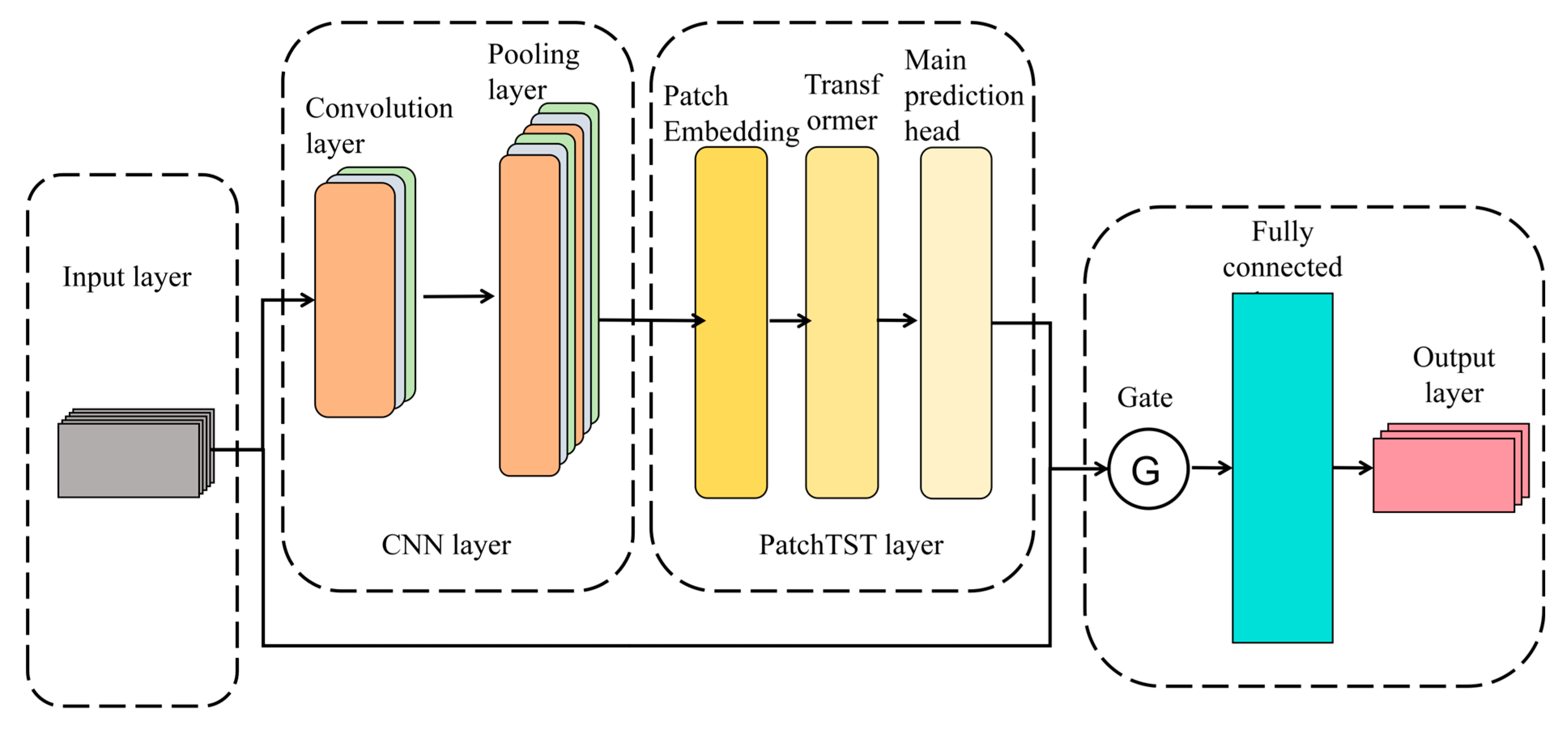
To address these limitations, particularly the challenge of persistent geometric drift inherent to small-radius curved alignments, we propose a 12-target, 5-step attitude prediction framework built on a hybrid CNN-PatchTST architecture with a gated inertial fusion mechanism. The framework unifies four elements within a single architecture: PatchTST’s global self-attention temporal encoding, CNN-based local feature extraction, a direct inertial mapping branch that explicitly models attitude continuity, and a learned gating module that adaptively balances inertial carry-forward against data-driven temporal correction. Unlike multi-objective optimization approaches that treat attitude targets through control-oriented objective functions, the proposed method produces simultaneous advance predictions for all 12 key attitude parameters over the next 5 steps (~4 min of lead time) in a purely predictive, deployment-ready form. SHAP attribution is further applied to construct a joint feature time-step matrix, revealing that the direct mapping branch accounts for approximately 97.7% of output variance, a finding that connects model behavior to known tunneling mechanics and provides operators with step-specific, quantifiable guidance for deviation correction.
3. Prediction Results
3.1. Shield Tunneling Data Collection
3.1.1. Project Overview
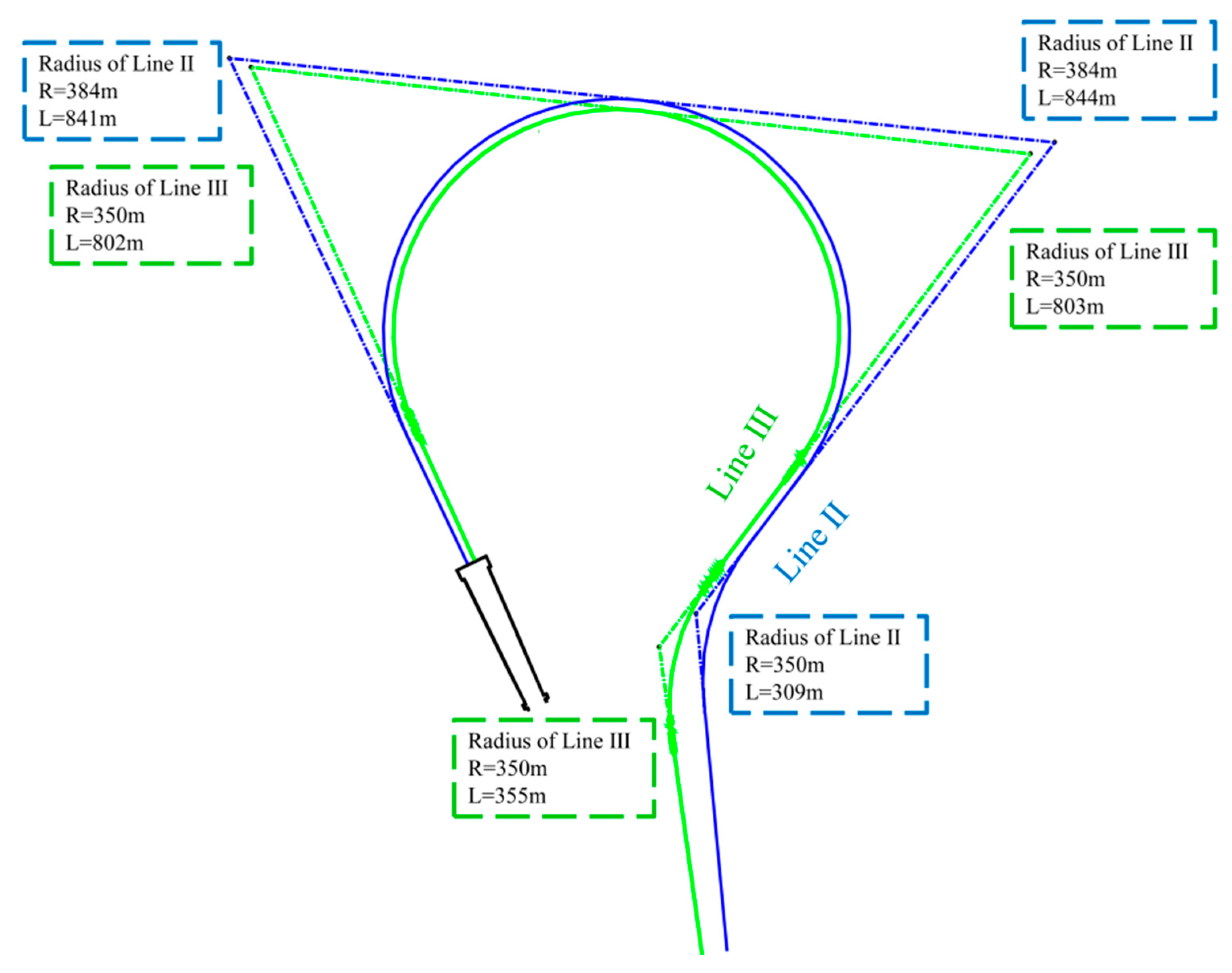
The model presented in this study is trained and validated on actual shield tunneling data from Work Area 7 of the Fangbai Intercity Railway, part of the Guangzhou Metro system. This work area comprises three shield tunnel sections: Lines II, III, and IV. Lines II and III together span approximately 2657.231 m, while Line IV extends roughly 2526.078 m. We select the Line III shield tunnel section as the primary research subject. Construction of Line III employed one slurry pressure balance shield machine with an excavation diameter of 8840 mm. The section has a minimum curve radius of 350 m and passes predominantly through strongly weathered rock, moderately weathered rock, limestone, gravelly sand, and silty clay, with karst cave encounters along the alignment. Line III requires continuous tunneling for more than 1.5 km under the 350 m curve radius. The alignment turns first right and then left at a small radius to form a bulb-shaped configuration, a layout rarely encountered in construction practice. The plan alignment of Line III section is shown in
Figure 3.
3.1.2. Data Collection
The attitude of a slurry pressure balance shield machine is directly influenced by multiple tunneling parameters spanning several functional systems. The thrust system contributes thrust jack pressure and stroke data. The cutterhead system supplies cutterhead torque, rotation speed, and penetration rate. The slurry circulation system provides feed and discharge flow rates, density, slurry chamber pressure, and air cushion pressure. The grouting system records synchronous grouting pressure. For attitude control, operators monitor 12 primary indicators: cutterhead horizontal and vertical deviations, articulation horizontal and vertical deviations, shield tail horizontal and vertical deviations, and the roll, pitch, and azimuth of both the front and rear shields. These parameters allow operators to continuously assess shield attitude and make prompt adjustments to keep the machine on the designed alignment while maintaining segment assembly quality and minimizing breakage and dislocation.
Relevant data from ring 1 to ring 1480 were collected and archived sequentially by ring number to serve as the input dataset.
Table 2 lists all input parameters.
A preliminary analysis of the dataset reveals that the standard deviation of the front and rear shield azimuths is approximately 96.65°, substantially larger than that of other angular parameters (standard deviation ≈ 0.44°). Over the entire alignment, the azimuth starts at roughly 330°, undergoes a transition from 360° to 0° near ring 268, and then increases monotonically from 0° to approximately 220°, accumulating a total change of about 250°. The 360°/0° boundary crossing occurs at a single data point (ring 268), which lies entirely within the training set; the validation and test sets span azimuth ranges of approximately 175–220° and 114.8–175.0°, respectively, neither of which crosses this boundary. Circular encoding (sin/cos representation) is therefore unnecessary.
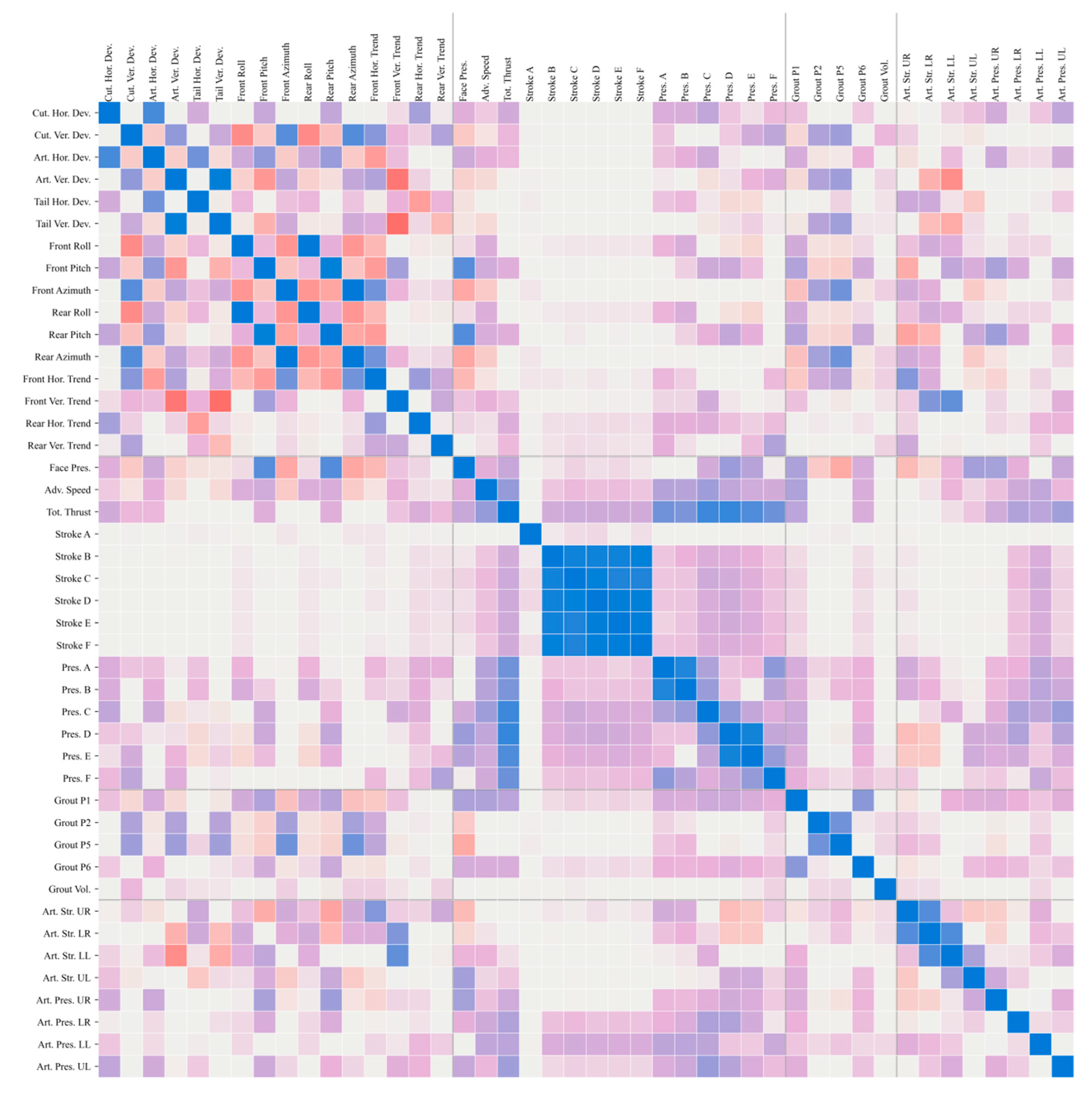
Pearson correlation analysis was used to evaluate linear correlations among the input parameters; the correlation matrix appears in
Figure 4. The Pearson correlation coefficient r ranges from −1 to +1, with larger absolute values indicating stronger linear correlation, as shown in Equation (5).
where r is the Pearson correlation coefficient;
Xi and
Yi are the i-th sample values of variables
X and
Y, respectively;
and
are the mean values of variables
X and
Y, respectively; and
n is the number of samples.
3.2. Data Preprocessing
Our data preprocessing workflow consists of five steps: shutdown filtering, outlier clipping, Savitzky–Golay (SG) smoothing, differential feature construction, and Z-score normalization. All statistics are computed solely on the training set before being applied to the validation and test sets, thereby preventing data leakage.
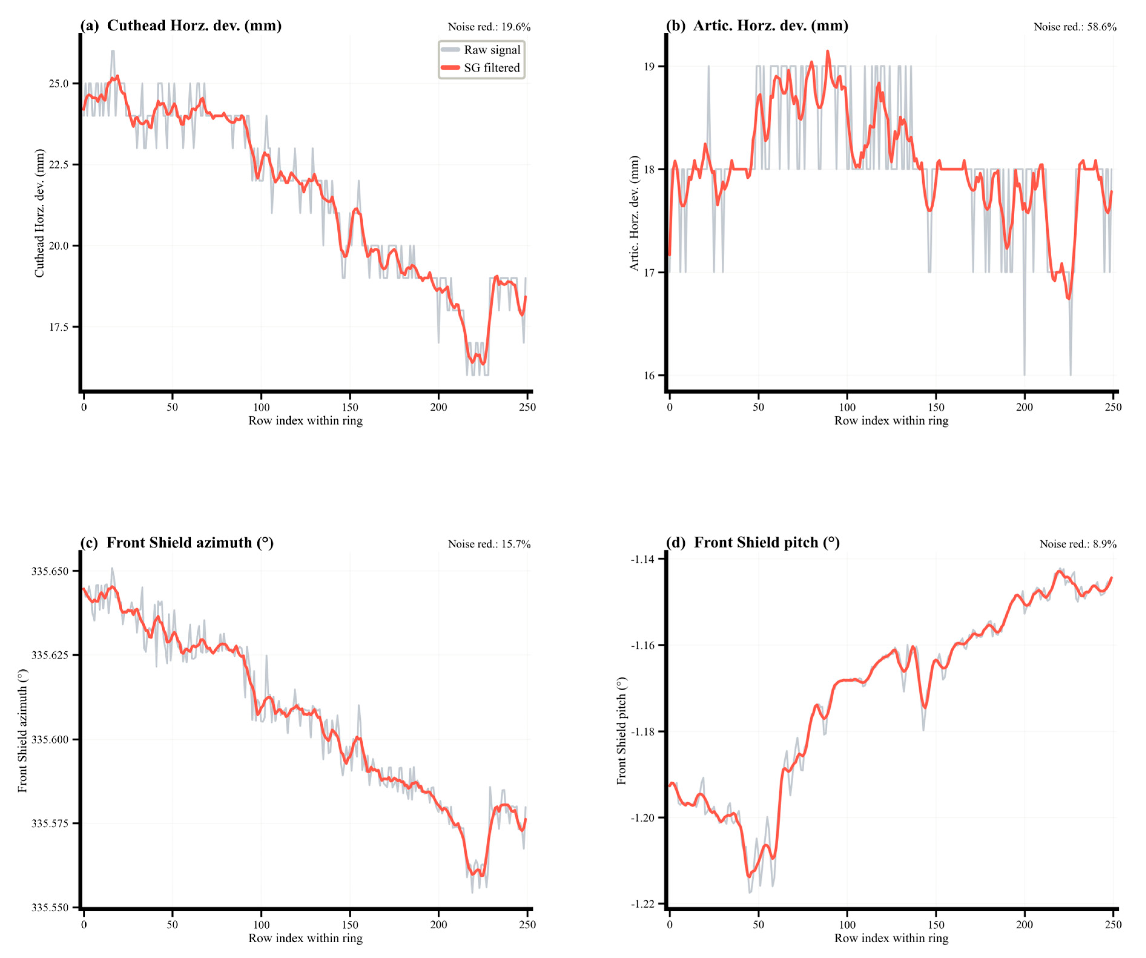
Shield tunneling generates substantial downtime data during activities such as segment assembly; these data carry no useful information for model training and must be removed. When the advance rate falls below 1 mm/min, we classify the corresponding time step as downtime and filter it out. The median inter-sample interval is 48 s (97th percentile: 52 s), so the sampling interval remains uniform after filtering, and five prediction steps continue to represent approximately 4 min of elapsed time. After filtering, the remaining 173,228 valid observations undergo 3σ outlier clipping: using the training-set mean μ and standard deviation σ, we set clipping boundaries at [μ − 3σ,μ+ 3σ] to eliminate noise. The signal is then smoothed with a centered SG filter (window length = 11, polynomial order = 3), as illustrated in
Figure 5. To prevent cross-split leakage, the SG filter is applied after the global temporal partition and independently within each ring of each subset.
We compute first-order temporal differences for each of the 12 target parameters to construct additional input features, as shown in Equation (6).
Physically, these differential features represent the instantaneous rate of change of each attitude parameter. They directly quantify the effect of each control adjustment and complement the original absolute-value features. Finally, both input and target parameters are normalized to zero mean and unit variance. Prediction results are mapped back to physical units via inverse transformation.
The dataset partitioning strategy is critical to model performance. We adopt a global temporal partitioning approach: the first 70% of the filtered data, in chronological order, is allocated to the training set; the middle 15% to the validation set; and the final 15% to the test set.
After partitioning, fixed-length input–output sequence pairs are extracted from the time-series data using a within-ring sequence partitioning method. A sliding window is applied independently within the data range of each ring, with a sequence length of L = 30, a prediction horizon of P = 5, and a sliding window stride of s = 3. Windows are never extracted across ring boundaries or across subset boundaries, so no input window contains observations from a different split. For the k-th ring with N
k valid rows, the number of extractable sequences is shown in Equation 7:
When Nk < L + P = 35, no sequences are generated for that ring, and it is skipped.
After the above processing, each sample consists of an input tensor and an output tensor, representing 30 consecutive steps of sensor history data and the next 5 steps of predicted attitude targets, respectively. The complete dataset spans 173,228 valid observations across 1477 rings. Following the 70/15/15 temporal split and within-ring sequence extraction, the training, validation, and test sets contain 31,620, 4768, and 5115 sequences, respectively, for a total of 41,503 sequences.
3.3. Evaluation Results
We trained the model using the optimized hyperparameters described above.
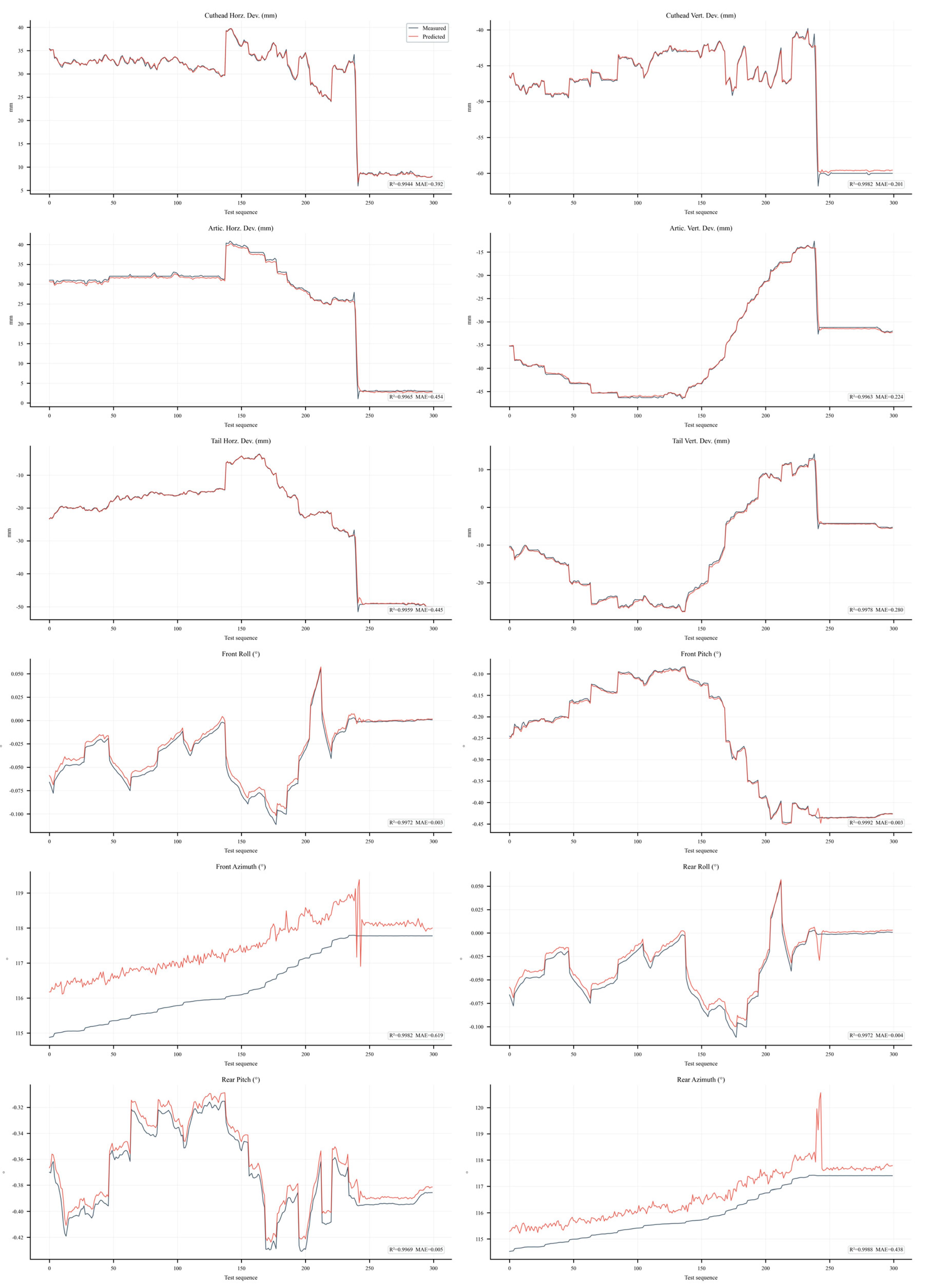
Figure 6 displays the prediction results. The predicted curves closely overlap with the measured data, and their trends are largely identical. The model achieves low RMSE and MAE values, with a mean R
2 of 0.992 across all 12 parameters; no individual parameter R
2 falls below 0.977. These results indicate strong fitting and generalization capabilities. To eliminate the effect of random parameter initialization, all metrics reported below represent the average of three independent training runs, with random seeds set to 42, 123, and 2024, respectively.
Table 3 summarizes the evaluation metrics.
3.4. Segment-by-Segment Evaluation
The held-out test set (rings 880–1200) lies entirely within the project’s continuous left-turn section, which features the most complex small-radius construction conditions and the most pronounced dynamic attitude variations along the entire alignment. The model achieves R2 = 0.992 on this test set, with azimuth MAEs of 0.536° and 0.392° for the front and rear shields, respectively, confirming reliable generalization to the most challenging conditions in this project.
To provide additional diagnostic insight into performance across different tunneling geometries, we also evaluated the model on the straight section (rings 1–208) and the right-turn section (rings 209–488). These segments fall predominantly within the training set and therefore do not constitute independent generalization tests; the results are reported as within-sample diagnostics only. Prediction accuracy on the straight and right-turn segments is higher than on the left-turn test set, consistent with the expectation that curved sections involve more complex attitude dynamics.
4. Model Performance Analysis
To verify the effectiveness of CNN-PatchTST for shield attitude prediction, we conduct two types of comparative analysis: ablation studies and model comparison experiments. In the ablation studies, individual modules are removed to assess their respective contributions. Specifically, we test performance after removing PatchTST, the direct mapping branch, and the gated fusion layer. In the model comparison experiments, we benchmark CNN-PatchTST against Long Short-Term Memory (LSTM), Gated Recurrent Unit (GRU), and CNN-LSTM.
4.1. Model Ablation Experiments
We conducted ablation studies to evaluate the functional role of each module.
Table 4 presents the results after removing PatchTST, the direct mapping branch, and the gated fusion layer, respectively.
The full CNN-PatchTST model achieves the lowest error across most metrics. One exception is azimuth MAE, where the No-Transformer variant (0.4488°) marginally outperforms the full model (0.4640°). This result suggests that for short-range azimuth prediction, the direct mapping branch alone may suffice; however, the Transformer component contributes to overall multi-target accuracy, particularly for positional deviation targets.
Removing the direct mapping branch caused severe performance degradation. Validation loss reached 0.113, while mean R2 dropped to 0.456 and azimuth R2 fell to a negative value (−1.621), with a corresponding MAE of 26.376°. These results indicate that the direct mapping branch plays a decisive role in multi-target attitude prediction. Position deviation R2 values, however, remained near 0.9. This suggests that the CNN-PatchTST main path has independently learned to predict position deviations from control parameters, even without the direct mapping branch.
Removing the gated fusion layer markedly degraded both training efficiency and fusion accuracy. When adaptive gated fusion was replaced with fixed-weight fusion, the model became substantially harder to converge: the optimal number of training epochs reached 252, and total training time extended to 71.2 min. Meanwhile, azimuth MAE rose from 0.464° (full model) to 1.455°. These outcomes confirm the essential role of adaptive gating in signal allocation. Fixed-weight allocation cannot adequately account for the dynamic variation of local and global features across different tunneling phases. The gating mechanism, by contrast, dynamically adjusts the fusion ratio of the two signal streams according to specific operating conditions, thereby accelerating convergence and improving prediction accuracy. An important practical implication follows: gated models are likely to converge more reliably to a stable solution when deployed under new operating conditions.
Removing the Transformer module (replacing it with an MLP) weakened the model’s resistance to long-term cumulative attitude drift. Roll and pitch MAE degraded from 0.0061° (full model) to 0.0085°. This finding underscores the importance of long-range trend modeling. At tunneling sites, roll and pitch drift typically manifest as high-frequency, small-amplitude fluctuations that accumulate over long periods. The Transformer’s self-attention mechanism effectively captures these long-range dependencies within the tunneling sequence; without it, the model cannot supply high-precision, timely responses to cumulative attitude drift.
In summary, the three modules contribute in distinct and complementary ways. The direct mapping branch supplies physical and geometric baseline constraints, preventing prediction collapse and substantially reducing azimuth error. Removing the gated fusion layer preserves dual-channel features but leads to extremely low convergence efficiency and poor multi-task coordination, precisely because adaptive signal allocation is absent. Removing the Transformer module strips the model of its capacity to capture global temporal dependencies, rendering it unable to track accumulated roll and pitch drift over long tunneling periods. The complete CNN-PatchTST model integrates the complementary strengths of all modules, achieving rapid convergence together with the highest prediction accuracy and optimal fitting capability.
4.2. Model Comparison Experiments
Table 5 presents a systematic comparison of LSTM, GRU, CNN-LSTM, PatchTST, Dlinear, Direct-mapping, Persistence and CNN-PatchTST for shield attitude prediction. CNN-PatchTST outperforms the other three models across all metrics.
GRU is the most competitive among the comparison models, with an overall R2 of 0.947. It achieves high accuracy (R2 = 0.92–0.99) for position deviation parameters such as cutterhead deviation and articulation deviation. For azimuth prediction, however, a clear shortcoming emerges: MAEs of 4.03° and 4.83° for the front and rear shield azimuths, respectively, are roughly 6.9 times higher than the corresponding CNN-PatchTST values (0.588° and 0.643°). This gap indicates that the GRU’s recurrent mechanism has limited capacity to model the long-range monotonic trend of azimuth angles.
LSTM performs substantially worse than GRU overall, with an overall R2 of only 0.175. The R2 values for the front and rear shield azimuths drop to −3.63 and −3.45, respectively, which is worse than a null model that simply outputs the mean.
CNN-LSTM records the poorest performance among the four models, with an overall R2 of −0.345, a mean MAE of 9.308, and azimuth R2 falling to −5.92. Notably, this model has more parameters (351,356) than CNN-PatchTST (263,732), yet its predictive performance is the lowest.
The shield azimuth varied monotonically from roughly 330° to approximately 220° over the entire alignment, accumulating about 250° of change and crossing the 360°/0° boundary near ring 268. In RNN-based models such as GRU and LSTM, the hidden-state recurrence mechanism operates strictly step-by-step: the hidden state at each step depends only on the previous hidden state and the current input, making direct long-range comparisons between distant time steps impossible. As the sequence length grows, long-range trend signals gradually attenuate during layer-by-layer recurrence. At the fine-grained scale of roughly 0.002° per step in azimuth change rate, this loss of long-range information prevents the model from identifying the current trend. It ultimately degenerates into an approximation that uses the recent local mean as its prediction. PatchTST’s self-attention mechanism, in contrast, allows the nine patches to attend to one another directly, enabling global comparisons that let the model identify sustained azimuth deviation trends.
To further contextualize the proposed model, we include four additional baselines. (1) Standalone PatchTST removes both the CNN front-end and the direct mapping branch, leaving only the patch-based Transformer. Its overall R2 collapses to 0.676, and azimuth R2 falls to −0.508, confirming that neither CNN local feature extraction nor the inertial prior can be omitted. (2) DLinear decomposes the 56-dimensional input into trend and seasonal components via moving-average filtering and maps each linearly; it achieves R2 = 0.973 but azimuth MAE of 2.42°, worse than CNN-PatchTST, indicating that linear mapping is insufficient for the nonlinear azimuth dynamics of curved alignment. (3) Direct mapping uses only the most recent 10-step attitude history via a two-layer MLP; at R2 = 0.988, it underscores the high inertia of shield attitude, yet azimuth MAE reaches 2.19°, which is 4.7× that of the full model. (4) Persistence simply copies the last observed attitude value to all five prediction steps, requiring no parameters. Its overall R2 of 0.993 and low mean MAE of 0.215 reflect the physically slow dynamics of shield attitude within the 4-minute window (median 5-step azimuth change = 0.012°) rather than a deficiency of the proposed model. Crucially, Persistence degrades 3.46× from Step 1 to Step 5 for position deviations, versus 1.92× for CNN-PatchTST, demonstrating that the proposed model maintains a more stable error profile at longer horizons. Furthermore, Persistence provides no mechanism for detecting impending attitude drift driven by control-parameter changes, a capability central to real-time tunneling correction.
To further examine model behavior across prediction horizons,
Table 6 reports position-deviation MAE at each of the five forecast steps for CNN-PatchTST and the Persistence baseline.
As expected, MAE increases monotonically with the prediction horizon for all models. CNN-PatchTST exhibits a Step-5/Step-1 degradation ratio of 2.16× for position deviation, compared with 3.46× for the Persistence baseline, indicating that the proposed model maintains more stable accuracy at longer horizons. GRU shows the smallest degradation ratio (1.15×), but its absolute position-deviation MAE at Step 1 already reaches 1.235 mm, which is 3.7 times that of CNN-PatchTST, confirming that low degradation alone is insufficient without a competitive starting accuracy.
4.3. SHAP Sensitivity Analysis
4.3.1. SHAP-Based Analysis Method
Deep learning models offer high predictive accuracy, yet their black-box nature makes it difficult for construction personnel to understand internal decision mechanisms, a limitation that restricts practical utility. To quantitatively reveal how various sensor input features influence shield attitude prediction, we employ the SHAP (SHapley Additive exPlanations) method for the interpretability analysis of the trained model.
Lundberg and Lee [
25] first proposed the SHAP method as a unified framework for interpreting machine learning model predictions. For the i-th feature in the feature set N, its SHAP value is defined as the weighted expected value of the average marginal contribution of that feature across all possible feature subsets, as shown in Equation (8).
where f(S) denotes the expected value of the model’s output when using only the feature subset S. Among existing feature attribution methods, SHAP provides one of the most rigorously grounded frameworks, rooted in cooperative game theory. It ensures that the contribution assigned to each input feature satisfies fairness and uniqueness axioms, making it a theoretically well-founded choice among additive attribution methods.
Given that CNN-PatchTST is a multi-layer nonlinear deep network, this paper employs the Gradient Explainer, which is suitable for neural network models. Because the output of CNN-PatchTST is a three-dimensional tensor, this paper constructs a single-target wrapper for each target parameter. The output of that target is averaged over five prediction steps and used as the scalar to be explained by SHAP. The SHAP value matrix is then calculated for each target in turn, where Ne = 30 is the number of explained samples, L = 30 is the historical sequence length, and D = 56 is the dimension of the input features.
4.3.2. Global Feature Importance Analysis
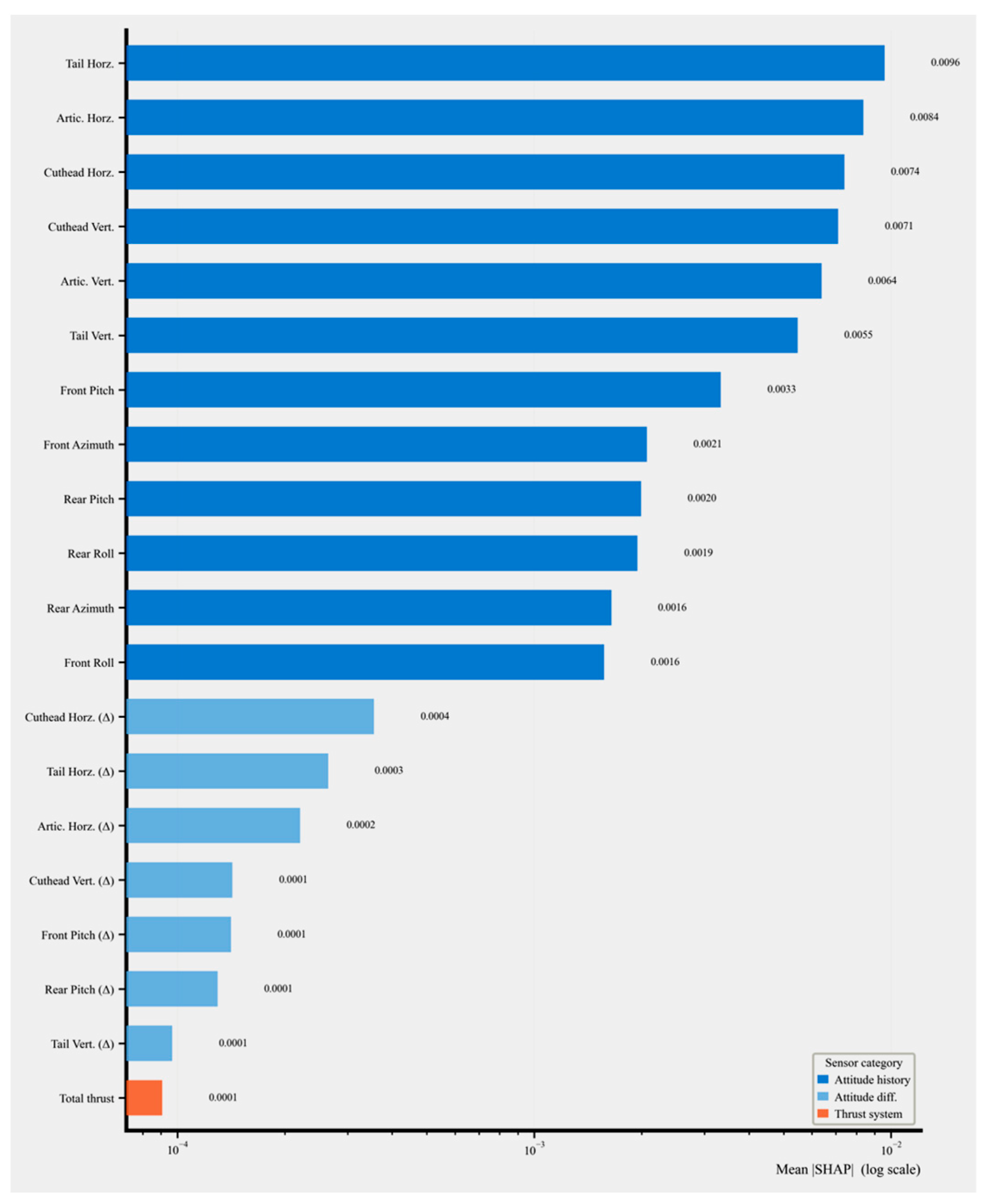
Figure 7 shows the SHAP sensitivity ranking for all input features. Historical values of attitude parameters dominate the most important features almost exclusively. Grouped by feature category, attitude parameters account for 97.3% of total contribution, while control parameters account for 2.7%. This distribution reflects a typical characteristic of shield tunneling data: the per-step attitude change of the shield machine rarely exceeds 0.1 mm, and the state between adjacent steps is highly continuous, making historical attitude the most predictive signal. To contextualize this finding, we evaluated a pure-inertia baseline (using only the direct mapping branch with historical attitude values) and obtained a mean R
2 of 0.988, only slightly below that of the full model. Position deviation R
2 matched that of the full model, but azimuth MAE reached 2.19°, which is 4.3 times higher than that of the full model. The reason is that azimuth prediction cannot rely solely on inertia; CNN-PatchTST can detect, through changes in control parameters, the moment when inertial tracking is about to break, thereby correcting the predicted orientation and improving accuracy.
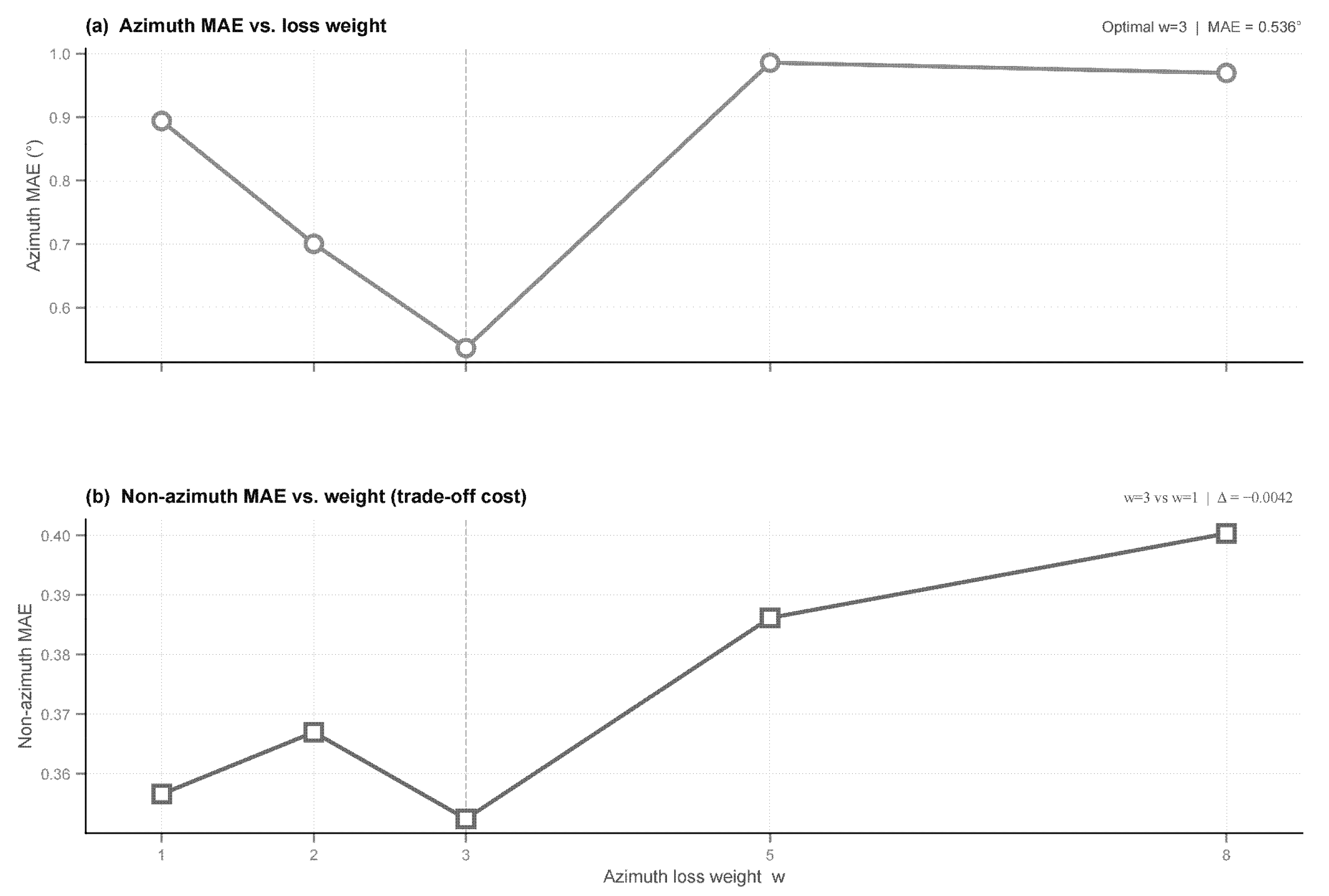
Table 7 reveals that the advantage of CNN-PatchTST over the inertial-only baseline grows consistently with the prediction horizon (MAE reduction: 14.8% at h = 1 to 42.4% at h = 4), with the most pronounced divergence occurring in azimuth prediction at h = 4 (192 s ahead), where the Only-Direct baseline’s azimuth MAE spikes to 2.056° compared with 0.452° for the full model—a 4.5-fold gap. This horizon-dependent degradation reflects the inherent instability of pure inertial extrapolation under small-radius curve conditions, where geological steering effects accumulate non-linearly beyond approximately three prediction steps.
4.3.3. Feature-Target Cross-Sensitivity Analysis
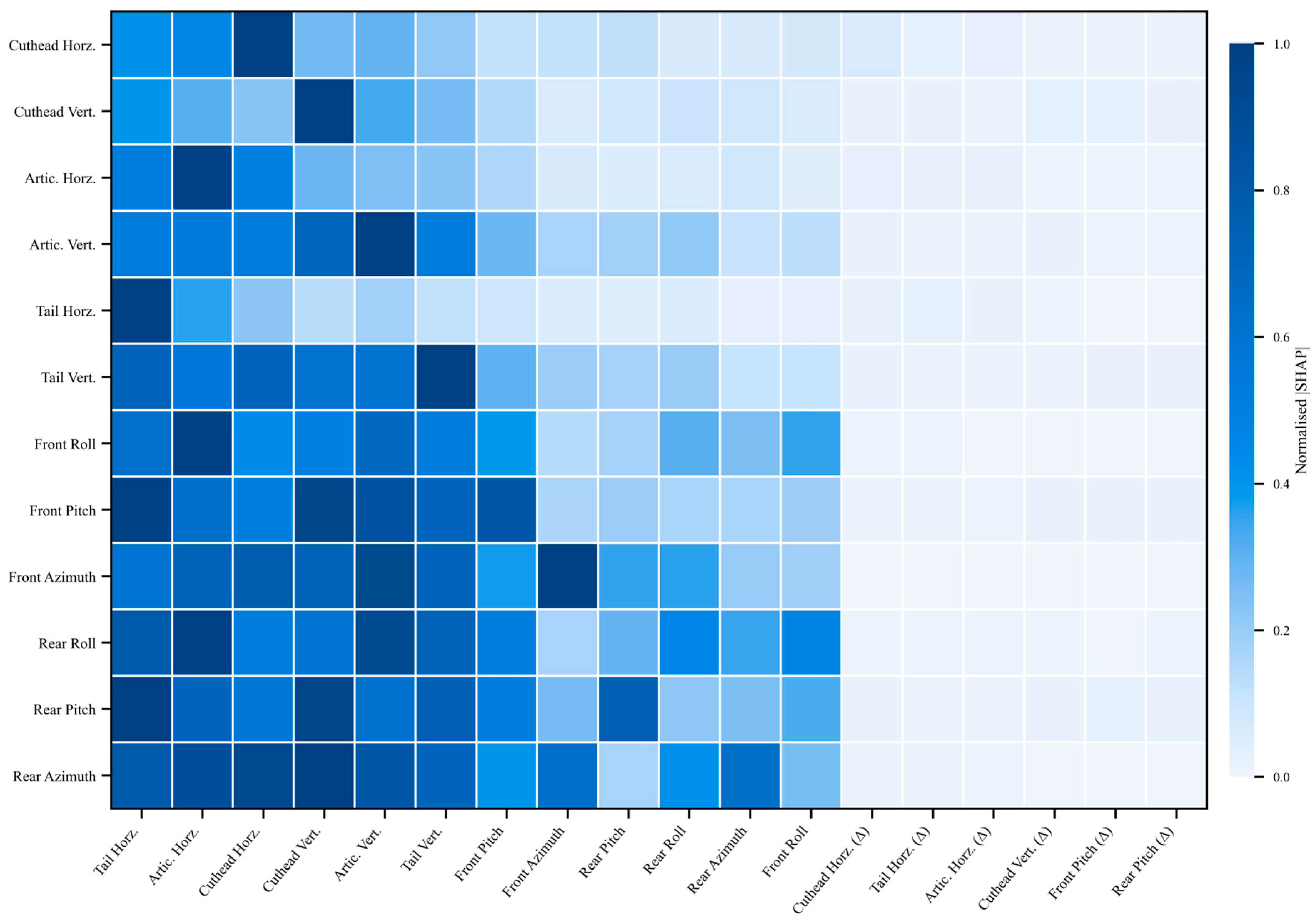
Figure 8 presents a 12 × 20 heatmap, where rows represent the 12 prediction targets and columns represent the 20 features with the highest global importance. Darker colors indicate a greater contribution of a feature to a target.
As expected, each attitude parameter’s prediction relies most heavily on its own historical values. A clear bidirectional contribution exists between cutterhead horizontal deviation and articulation horizontal deviation, forming a dark region spanning two rows on the heatmap. Because the three sections of the shield machine are rigidly connected, the cutterhead, articulation, and shield tail drive one another during horizontal deflection, and their historical data are naturally correlated. In the Pearson correlation analysis, the coefficient between these two parameters is r = 0.766, one of the highest among all feature pairs. Articulation vertical deviation exhibits a different pattern: in addition to contributing most strongly to its own prediction, it also makes a particularly significant contribution to front shield pitch. The differential vertical stroke of the articulation jacks is strongly associated with the relative pitch angle between the front and rear shields (r = −0.661), consistent with the mechanical coupling of the articulation system. Azimuth trend appears relatively independent of other parameters; non-diagonal regions are generally lighter in color, and azimuth prediction relies almost exclusively on its own historical trend.
4.3.4. Recency Effect Analysis
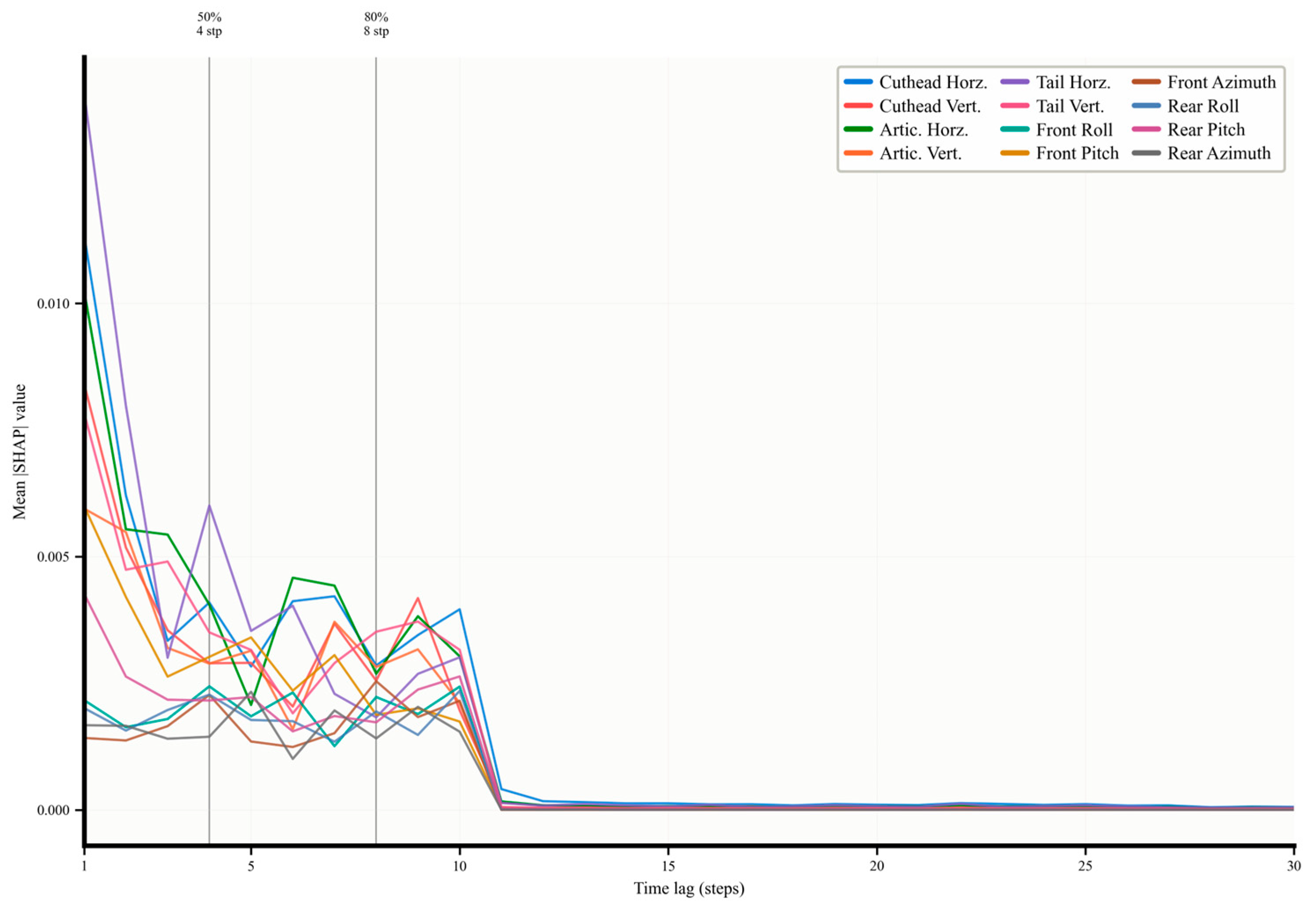
Figure 9 displays the 30-step historical sequence in chronological order, where lag = 1 represents the most recent step and lag = 30 the most distant. Importance peaks at lag = 1 for all parameters, then decays rapidly, approaching zero and stabilizing near lag = 20. Importance at lag = 1 is 313.7 times that at lag = 30. The most recent 4 steps account for 50% of total importance, and the most recent 10 steps cumulatively account for 90%; all historical steps with lag > 20 collectively contribute only 0.9%.
The rate of decline varies among different target parameters. SHAP values for position deviation parameters are highest in the most recent steps and decline the fastest, indicating greater sensitivity to recent operations. Curves for azimuth and pitch are relatively flatter, retaining some significance near lag = 15, which suggests that angular parameters exhibit longer predictive memory in the model’s attribution patterns.
5. Conclusions
This study addresses two challenges in shield attitude prediction for small-radius curved tunneling: insufficient multi-step prediction accuracy and limited interpretability. We propose a hybrid deep learning model based on CNN-PatchTST and conduct a multi-factor sensitivity analysis using the SHAP method. Validated on construction data from the Guangzhou Metro Fangbai Intercity Railway (minimum curve radius 350 m), the main findings are as follows:
(1) The CNN-PatchTST main branch learns the dynamic mapping between control parameters and attitude; the direct mapping branch provides short-step inertial estimates using pure attitude history; and the gated fusion layer achieves adaptive integration of the two signal streams. Under three independent random seed initializations, the model achieves a mean R2 of 0.9921 ± 0.0003 across all 12 attitude parameters. Position deviation MAEs range from 0.33 to 0.82 mm, angular MAEs for roll and pitch are below 0.005°, and azimuth MAEs reach 0.54° and 0.39° for the front and rear shields, respectively. The small standard deviation indicates that model performance is insensitive to parameter initialization.
(2) Ablation studies confirm the complementary roles of each module. Removing the direct mapping branch causes mean R2 to collapse and azimuth prediction to fail. Replacing the Transformer encoder with an MLP degrades roll and pitch prediction errors by 39%, validating the necessity of global self-attention for modeling long-term cumulative drift. Disabling gated adaptive fusion increases training time by approximately 10% and degrades azimuth MAE by 171%, indicating that the core value of the gating mechanism lies in adaptively balancing contributions from the two signal paths, rather than merely improving overall fitting accuracy.
(3) SHAP analysis reveals that historical attitude parameters account for approximately 97% of feature importance. The recency effect shows that the four most recent steps contribute over 50% of total predictive power, and the cumulative contribution of the most recent 20 steps reaches 99%. This finding suggests that retaining only the most recent 20 steps of data may suffice for normal prediction, a useful reference for lightweight on-site deployment. At the control parameter level, the thrust jack pressure differential shows the strongest predictive association with cutterhead horizontal deviation among all control features. The SHAP attribution pattern further reveals that this association leads articulation and shield tail deviations by approximately 3–4 steps (roughly 3–4 min); this pattern may offer operators a qualitative reference for proactive pressure adjustment, though its causal interpretation requires further validation.
The findings of this study carry several practical implications for shield tunneling engineering. Accurate multi-step attitude prediction can directly support real-time steering control: prior work has demonstrated that embedding a deep learning prediction model within an online multi-target multi-step optimization framework reduces overall trajectory deviations by up to 46.4% [
11]. The proposed CNN-PatchTST framework, with its 5-min advance horizon, is architecturally compatible with such closed-loop control pipelines, and its simultaneous prediction of all 12 attitude parameters may further benefit multi-target multi-step steering strategies for large-diameter shield machines [
31]. Beyond attitude control itself, the downstream consequences of uncorrected attitude deviation are substantial: field monitoring of sequential twin-tunnel construction has shown that shield attitude irregularities contribute measurably to ground settlement and associated carbon emissions [
32]. By enabling earlier and more targeted correction, the proposed method may help reduce these environmental and safety costs. At the deployment level, the SHAP recency analysis indicates that retaining only the most recent 20 steps of sensor history suffices for normal prediction, suggesting that the framework can be implemented in lightweight on-site systems without sacrificing accuracy.
The model has been validated on data from a single project, a single slurry pressure balance shield machine, and a single sensor configuration. The training, validation, and test sets share the same machine, geology, and construction team; therefore, the reported performance should be interpreted as evidence of within-project generalization rather than cross-project transferability. In terms of computational efficiency, the trained model requires approximately 2.6 ms per inference on an Intel i7-12700H CPU (batch size = 1) and approximately 1.5 ms on an NVIDIA GeForce RTX 4060 Laptop GPU, well within the 48-s data acquisition interval. The reported inference latency demonstrates computational feasibility for real-time operation but does not constitute a validated field deployment. Full deployment additionally requires integration with the PLC sensor stream, an online Savitzky–Golay preprocessing pipeline, and monitoring for distribution shift as geological conditions change. However, aspects such as online data availability, sensor fault tolerance, and robustness under distribution shift remain to be evaluated. Formal cross-model statistical significance testing requires multi-seed baseline evaluations. Future work may explore transfer learning and domain adaptation across different tunnel alignments and shield machine types to enhance engineering generality. Incorporating geological indicators as additional input features is expected to further improve model robustness under varying strata conditions.