1. Introduction
Industrial plant construction projects involve interdependent systems, complex spatial interfaces, and strict execution constraints that must be carefully coordinated during early planning stages [
1]. To support such coordination, data-rich models are needed to represent not only the physical components involved in construction but also their planned timing and installation sequence [
2,
3,
4]. Four-dimensional Building Information Modeling (4D BIM) addresses this need by integrating 3D model components with construction schedule data, allowing construction progress to be visualized over time [
5]. This integration also provides an important foundation for contemporary construction planning practices, including Advanced Work Packaging (AWP) [
6,
7].
Given these demonstrated benefits, 4D BIM-based approaches have been successfully applied to detect and resolve spatiotemporal clashes in underground pipeline construction [
8] and to support decision-making for site layout optimization in mega LNG plant construction [
9]. Additionally, a recent review of the role of BIM in industrial plant construction synthesized a broader range of 4D BIM-enabled applications, including constructability review, progress monitoring, and collaborative planning [
10]. However, despite these advancements, the practical application of 4D BIM for detailed construction planning remains hindered by several limitations. A primary challenge is the granularity mismatch between construction schedules, which are often organized at activity or work-package levels, and 3D BIM models, which contain more detailed model components [
11]. This mismatch becomes particularly problematic in plant piping systems, where a single installation work package (IWP) may encompass multiple isometric drawings, each of which can be further decomposed into spools and individual BIM components [
12]. Furthermore, the installation sequence of these individual components is often governed by topological and spatial constraints, such as component connectivity, containment, and relative component locations. For example, physical connections between components can create installation interdependencies that constrain their sequencing [
3]. Spatial constraints may require pipe welding to precede the installation of nearby electrical trays that would obstruct the welding workspace [
10]. However, broad construction schedules typically do not provide the component-level precedence logic required to represent these constraints [
12]. Consequently, the object-level groupings, installation logic, and spatial dependencies required for detailed construction planning often have to be manually interpreted based on human experience [
6,
13]. Furthermore, identifying individual components within a given work scope and organizing them into appropriate installation groups and sequences remain time-consuming, often requiring tedious manual inspection and selection of components piece by piece [
4,
11].
Several studies have sought to address these limitations by deriving object-level relationships from BIM models. For example, geometric approaches have used 3D surface meshes to infer missing spatial and topological links between model components. Mesh-level spatial operations, however, have been shown to impose substantial computational costs, particularly in large-scale models [
14]. Simplified geometric representations, such as bounding boxes, can reduce this burden, but previous studies have found that they may introduce false-positive connections, especially in spatially congested areas [
15]. These limitations indicate the need for a method that combines geometric and semantic data to derive reliable object-level connectivity and support its subsequent use in detailed construction planning.
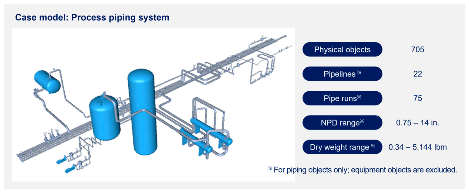
Therefore, this study aims to develop a method for generating installation sequences from object-level BIM data of plant piping systems to help bridge the granularity gap between construction schedules and BIM model objects. The proposed method combines lightweight bounding-box geometry with piping-specific semantic information to derive the object-level relationships required for installation grouping and sequencing. Candidate adjacency relationships are first identified using AABB-based spatial queries and subsequently refined through geometric and semantic false-positive filtering to establish validated object-level connectivity. Based on the resulting connectivity graph, individual piping objects are organized into dimensionally feasible installation groups by considering Pipeline and PipeRun information, connectivity, and dimensional constraints. Finally, predefined priority rules are applied to the generated groups to determine candidate installation sequences. The proposed method is implemented as a custom Autodesk Navisworks add-in, enabling the required geometric and semantic information to be directly extracted and processed within the BIM environment.
The remainder of this paper is organized as follows.
Section 2 reviews previous studies related to object-level connectivity, grouping, and installation sequencing.
Section 3 presents the proposed methodology for connectivity inference, installation grouping, and sequence generation.
Section 4 presents the case-study implementation and the resulting connectivity, grouping, and sequencing results.
Section 5 discusses the findings and implications of the proposed method.
Section 6 summarizes the main conclusions, limitations, and directions for future research.
2. Literature Review
2.1. Geometric and Semantic Connectivity Inference
Deriving object-level relationships from 3D BIM models is a prerequisite for interpreting how model components interact in space and how they can be used in downstream construction-planning applications. One approach to obtaining such connectivity information is to use explicit relationship entities predefined within the Industry Foundation Classes (IFC) schema, such as IfcRelConnectsElements or IfcRelConnectsPorts [
15,
16]. However, relying solely on explicit connectivity relationships encoded in IFC is often impractical for real-world projects. Previous studies have pointed out that these relationship entities are frequently empty or incomplete in actual IFC files due to modeling omissions, errors, or information loss during data exchange between different BIM authoring tools [
14,
16].
To address the absence of explicit connectivity links, several studies have attempted to infer spatial or topological relationships directly from the geometric representations of 3D objects. For example, Lilis et al. [
14] reconstructed missing topological links in complex MEP networks by using 3D surface meshes from BIM objects to compute spatial intersections and adjacencies. However, computing spatial relationships directly from detailed 3D meshes incurs high computational costs, especially in large-scale BIM models containing thousands of complex elements. Furthermore, since precise mesh operations are highly vulnerable to surface modeling errors, bounding box collision checks are often required as a supplementary step to capture missing connections. To reduce this computational burden and improve robustness to geometric imperfections, Emunds et al. [
15] relied on bounding-box-based representations, rather than detailed mesh-to-mesh intersection checks, to infer candidate spatial relationships. Although this approach successfully generated candidate connection edges for MEP networks, the study also noted that bounding-box-based spatial queries can introduce extraneous edges and false-positive relationships, particularly in dense areas where multiple components are located in close proximity.
Therefore, domain-specific semantic properties can be incorporated to reduce false-positive relationships while retaining the lightweight advantages of bounding-box-based inference. These properties can constrain whether a detected spatial relationship represents a genuine topological connection rather than spurious spatial proximity between incompatible component types. In industrial piping systems, relevant semantic properties may include pipeline and pipe run hierarchy, component types such as pipes, elbows, tees, and valves, and the expected port count for each component type [
15,
17,
18]. These domain-specific constraints provide a promising basis for refining geometry-derived adjacencies. Building on these findings, the present study combines lightweight geometry-derived adjacencies with piping-specific semantic constraints and uses the refined connectivity for object grouping and candidate installation sequencing.
2.2. Connectivity-Based Object Grouping
In industrial plant projects, the AWP framework progressively structures construction scope into Construction Work Areas (CWAs) and Construction Work Packages (CWPs), which are subsequently developed into Installation Work Packages (IWPs) for field execution [
19,
20]. Translating these planning units into detailed installation plans, however, may require individual piping components to be further organized into manageable intermediate groups. The criteria used to form such groups should reflect the intended purpose of the resulting units [
21]. Physical connectivity can identify components that may be grouped together, but it does not by itself determine suitable group boundaries. For installation planning, these boundaries should also account for construction-related requirements so that the resulting groups can be handled and assembled under practical field conditions.
Research on component grouping has followed two related directions. At the work-package level, Isaac et al. [
3] proposed a bottom-up method that analyzed topological relationships and construction sequences, initially assigned components according to the resources required for their installation, and refined the resulting packages to reduce workflow interruptions and inter-package interfaces. At the module level, Samarasinghe et al. [
21] combined a Dependency Structure Matrix and hierarchical clustering to identify modules in chilled-water plantroom systems while considering module dimensions, mass, handling limitations, and the complexity of onsite assemblies. More recently, Zhao et al. [
22] applied genetic-algorithm-based partitioning to integrated corridor pipelines using constraints related to module length, costs, connector locations, transportation, and lifting requirements.
Taken together, these studies show that the grouping of detailed components into construction-planning units should be aligned with the intended level and purpose of construction planning. At the work-package level, such grouping may be guided by component and activity relationships, resource requirements, and workflow interfaces, whereas object-level physical grouping may additionally consider dimensions, weight, and connection characteristics. Connectivity therefore provides a structural basis for component grouping, while the practical boundaries of the resulting groups should reflect their intended construction use and associated physical constraints.
2.3. Rule-Based Installation Sequencing
Once individual piping objects have been organized into installation groups, the relationships among the groups can be translated into a candidate installation sequence. Connectivity identifies which components are physically related, but it does not by itself determine a unique installation sequence. Different sequences may be generated from the same connectivity structure depending on the starting point, branch priority, spatial configuration, construction method, and other project-specific requirements.
In this regard, previous studies have attempted to automate detailed installation sequencing and dependency analysis by applying rules tailored to their respective construction contexts. To ensure worker accessibility and prevent interference in constrained spaces, Isaac and Shimanovich [
23] prioritized components located farther from workers, such as those closer to ceilings or positioned behind other components. Similarly, Singh et al. [
24] applied “higher-to-lower” and “outer-to-inner” sequencing rules to coordinate closely spaced pipe systems installed near ceilings and walls. In a different context, Yin et al. [
8] imposed constraints requiring pipeline removals to precede new installations to resolve spatiotemporal clashes during underground pipeline relocations.
These studies indicate that installation sequencing is context-dependent, as differences in spatial configuration, construction methods, and project requirements may result in different sequencing priorities. A practical sequencing method should therefore allow the applicable work scope and priority criteria to be adjusted rather than prescribe a single universal sequence. The selection and relative priority of these criteria are project-specific planning decisions. Once the criteria are specified, identifying equipment-connected starting candidates, comparing pipe diameters and elevations, and selecting connected successor groups can be automated using BIM-derived information. Accordingly, this study applies predefined project-specific priority rules to generate candidate installation sequences among connectivity-based installation groups.
3. Methods
3.1. Overview
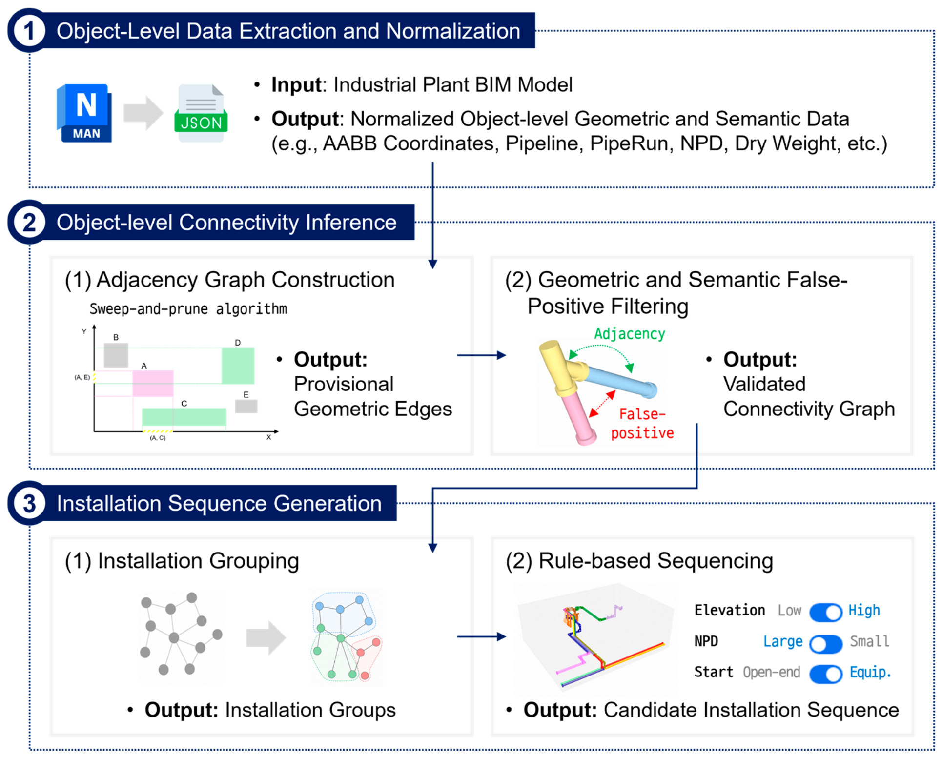
The proposed framework is organized into three phases comprising five sequential stages, as illustrated in
Figure 1. First, object-level geometric and semantic information is extracted from the Navisworks model and normalized for consistent component identification. Second, candidate adjacency relationships are generated from AABB geometry using a sweep-and-prune algorithm and represented as an object-level geometric adjacency graph. Third, geometric and piping-specific semantic rules are applied to remove false-positive relationships and establish validated object-level connectivity. Fourth, the validated connectivity graph is used to form installation groups by considering Pipeline and PipeRun properties, connectivity, and dimensional constraints. Finally, predefined priority rules are applied to the resulting groups to generate a candidate installation sequence. The framework is implemented within Autodesk Navisworks, allowing data extraction, connectivity inference, grouping, and sequencing to be performed within a consistent BIM environment.
3.2. Object-Level Data Extraction and Normalization
Geometric and semantic data are directly extracted from each object in the Navisworks model. As summarized in
Table 1, object geometry is represented using an axis-aligned bounding box (AABB), defined by the minimum and maximum coordinates along the global X, Y, and Z axes. The six AABB coordinates,
, are extracted in the global model coordinate system using the native units of the source model. The extracted semantic data include the object GUID, pipeline, pipe run, nominal pipe diameter (NPD), dry weight, flow direction, display name, short code, and description. The GUID uniquely identifies each model object and enables consistent object-level matching throughout subsequent processing. The Pipeline property identifies the broader piping system to which an object belongs, whereas the PipeRun property denotes a more detailed run within the corresponding pipeline. The display name, short code, and description are used to identify the component type, while the remaining properties are retained for subsequent connectivity validation and component-grouping analyses.
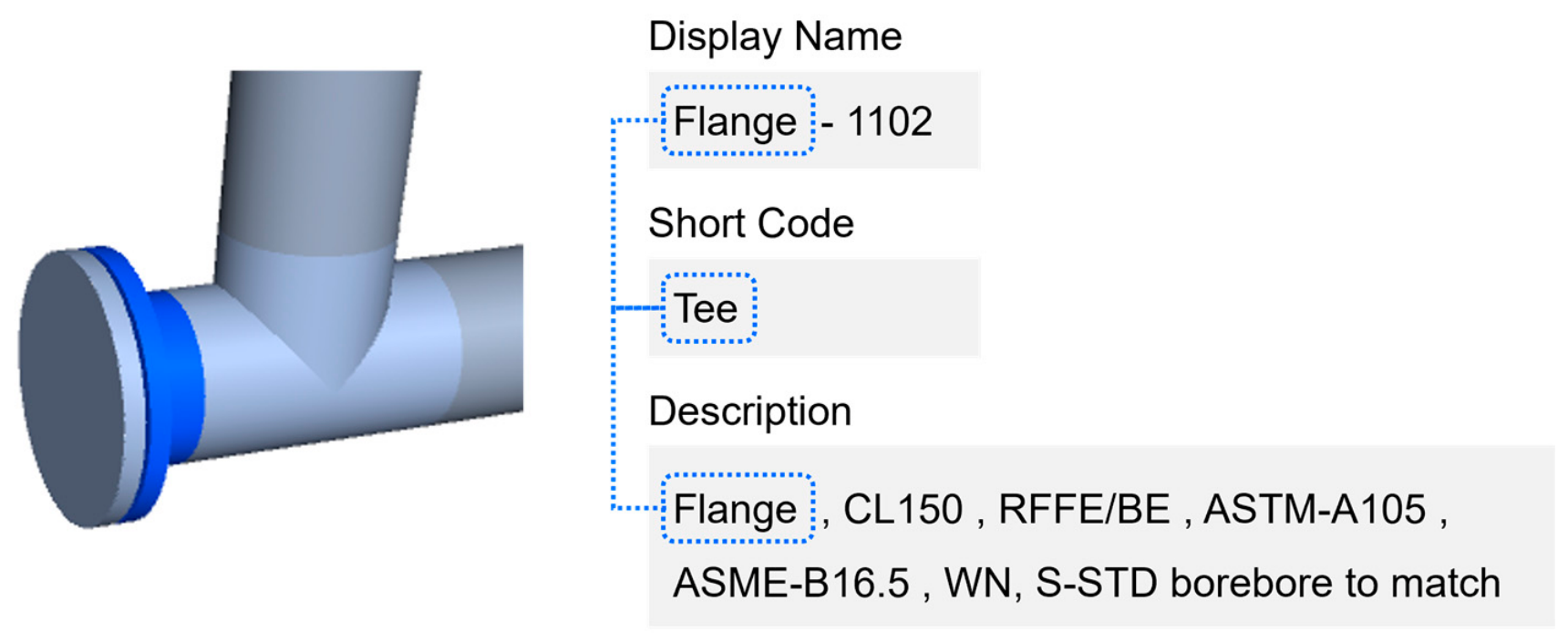
For component-type identification, the short code is treated as the primary source-model property. However, this property may be blank or inconsistent with the actual component type for some objects. It is therefore compared with the display name and the description prefix, defined as the text preceding the first comma in the description. Specifically, the three text properties are normalized by removing leading and trailing whitespace and using case-insensitive matching before component classification. Trailing object serial numbers matching the pattern -\d+$ are additionally removed from display names. For example, Flange-1102 and VG317-0101 are normalized to Flange and VG, respectively. Each normalized string is then mapped to a standardized component type using a predefined dictionary. When multiple expressions could match the same string, the more specific expression is applied. Consequently, synonymous expressions such as ‘90 deg LR elbow’, ‘90 deg elbow’, and ‘90E’ are mapped to the standardized component type ‘90 Degree Direction Change’.
After normalization, a majority-voting rule is applied to determine the final component type. When at least two of the three normalized properties—the display name, short code, and description prefix—support the same standardized type, that type is assigned to the object. When neither the short code nor the description prefix contains a valid value but the normalized display name yields a valid type, the type inferred from the display name is retained. Objects for which the available properties produce conflicting results without sufficient agreement are flagged for manual review. Each standardized component type is also associated with an expected port count for use in the subsequent connectivity validation process.
Figure 2 illustrates the normalization and majority-voting procedure using an example object. Despite the conflicting short code, agreement between the display name and description prefix results in the final classification of ‘Flange’.
3.3. Geometric Adjacency Graph Construction
A geometric adjacency graph
is constructed to represent candidate spatial relationships among piping objects. Each object with a valid AABB is represented as a node, and an edge is established between two nodes when their bounding boxes satisfy one of the predefined geometric adjacency conditions. To improve computational efficiency and avoid evaluating all possible object pairs, candidate pairs are first generated using a sweep-and-prune algorithm [
25]. As detailed in Algorithm 1, objects are sorted in ascending order of their
coordinates and sequentially processed using an active set. An object is removed from the active set when its
coordinate is more than the candidate search tolerance behind the
coordinate of the current object. For each remaining object in the active set, the AABB separations along the Y and Z axes are calculated. A pair is retained as a candidate only when both separations are within the candidate search tolerance. Candidate pairs are stored without regard to object order, preventing duplicate representation of the same object pair.
| Algorithm 1. Sweep-and-prune-based candidate-pair generation algorithm. |
| Input | |
| Output | unordered candidate-pair set
|
and candidate-pair set as empty.
do
do
5: ←
6: ←
then
9: end if
10: end for
12: end for
|
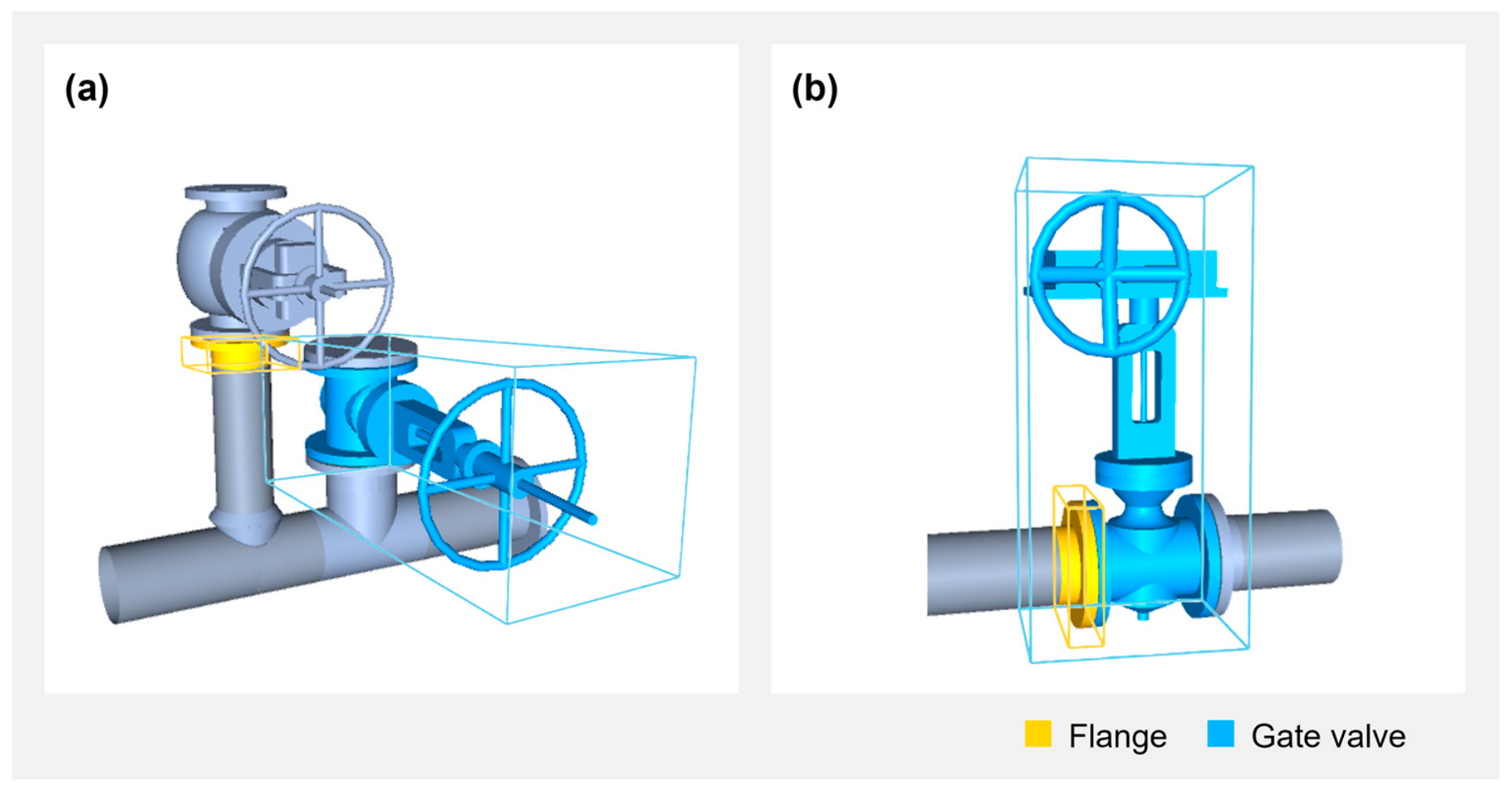
For each candidate pair in , the spatial relationship between the corresponding AABBs is determined based on the signed overlap along each principal axis. A positive value indicates that the two AABB intervals overlap along the axis, a value of zero indicates contact, and a negative value indicates separation. Values whose absolute magnitudes fall within a predefined numerical tolerance are set to zero to prevent floating-point errors from affecting the relationship classification. The numerical tolerance was set to 0.0001 in., a sufficiently small value used only to suppress floating-point noise around zero rather than to represent a physical clearance.
Next, the spatial relationships of candidate pairs are classified by adapting the disjoint, touch, and overlap relations established for three-dimensional spatial objects to AABB-based criteria [
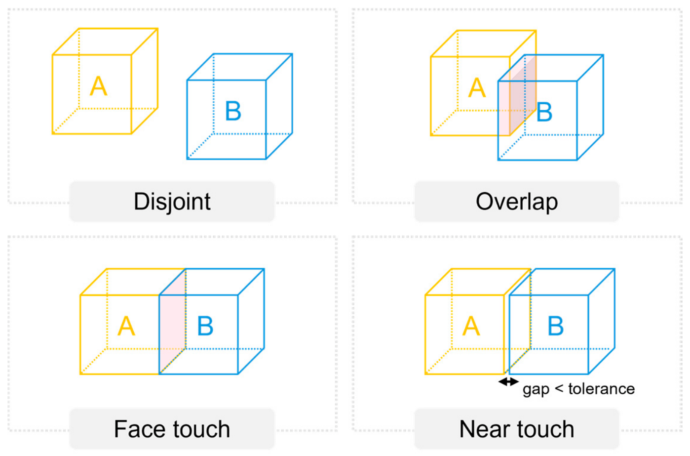
26]. Because small geometric gaps may exist between elements in BIM models, the conventional touch relation is subdivided into face touch, representing exact boundary contact, and near touch, representing separation within a predefined gap tolerance [
15]. Accordingly, the four relationships are defined as follows and illustrated in
Figure 3. In this classification, overlap is assigned when the signed overlaps along all three axes are positive. Face touch is assigned when exactly one signed overlap is zero and the other two are positive. Near touch is assigned when exactly one signed overlap is negative but remains within the predefined gap tolerance, while the other two are positive. All remaining configurations are classified as disjoint. For the implementation, the near-touch gap tolerance was derived from the small separation observed between directly connected flange pairs, which was approximately 0.125 in. A tolerance of 0.25 in., approximately twice this value, was adopted to accommodate comparable geometric discrepancies. The candidate search tolerance, in turn, was set to 0.75 in., which is larger than the near-touch tolerance, to avoid prematurely excluding potentially valid pairs while limiting the number of pairwise evaluations.
3.4. Geometric and Semantic False-Positive Filtering
Although AABB-based spatial relationships provide an efficient means of identifying geometrically adjacent objects, geometric proximity alone does not necessarily indicate direct physical connectivity, particularly in congested piping areas. Therefore, candidate pairs classified as disjoint are excluded from further analysis, whereas those classified as overlap, face touch, or near touch are retained as provisional geometric edges. These provisional edges are then evaluated using the three false-positive filtering rules summarized in
Table 2.
Geometric validity checks are first applied to verify that the computed spatial measures satisfy fundamental geometric bounds. For example, an overlap volume cannot exceed the volume of either participating AABB; any edge violating this condition is classified as geometrically invalid and excluded.
For recurrent component-type pairs, the remaining edges are grouped by component-type pair, and their geometric relationships and overlap characteristics are compared within each group. For example, for flange–gate valve pairs classified as overlap, overlap volumes were log-transformed and evaluated using the interquartile range (IQR). Log-transformed values more than 1.5 times the IQR below the first quartile were regarded as lower outliers and flagged for manual review.
Following geometric filtering, semantic compatibility rules based on component types are applied to remove edges that are inconsistent with the expected direct connection configurations of the piping system. These rules encode piping domain knowledge by specifying the permissible counterpart types for selected component types. For example, in the adopted object representation, a sockolet is treated as a branch outlet connected directly to a pipe or nipple. Similar interface-based constraints are applied to spectacle blinds, blind flanges, and gate valves. The semantic compatibility rules adopted in this study are summarized in
Appendix A (
Table A1). These rules were defined for selected component types with constrained direct-connection configurations; component types not listed in
Table A1 were not automatically treated as incompatible.
Finally, the retained edges are evaluated using expected port-count constraints as an additional topological consistency criterion. Each standardized component type is assigned a predefined expected port count, as summarized in
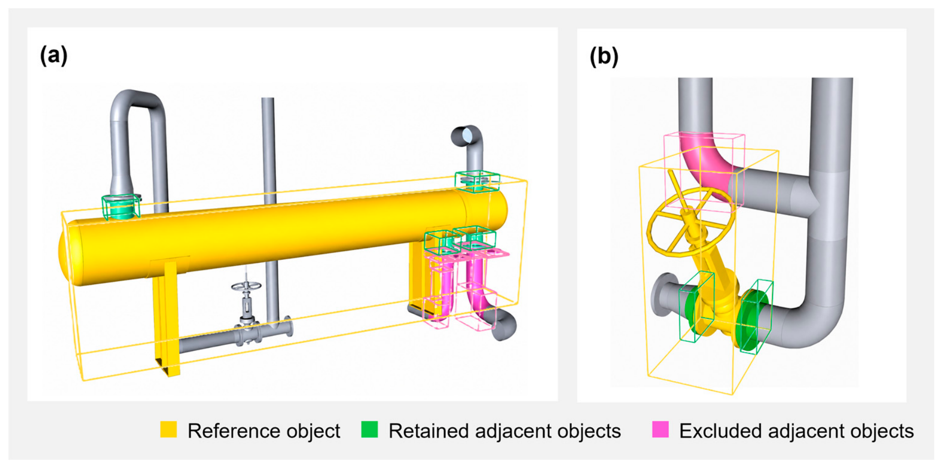
Table 3. The observed port usage is not determined simply by the number of adjacent objects. Instead, only adjacencies corresponding to valid connection directions of the target object are included, resulting in a direction-adjusted port count.
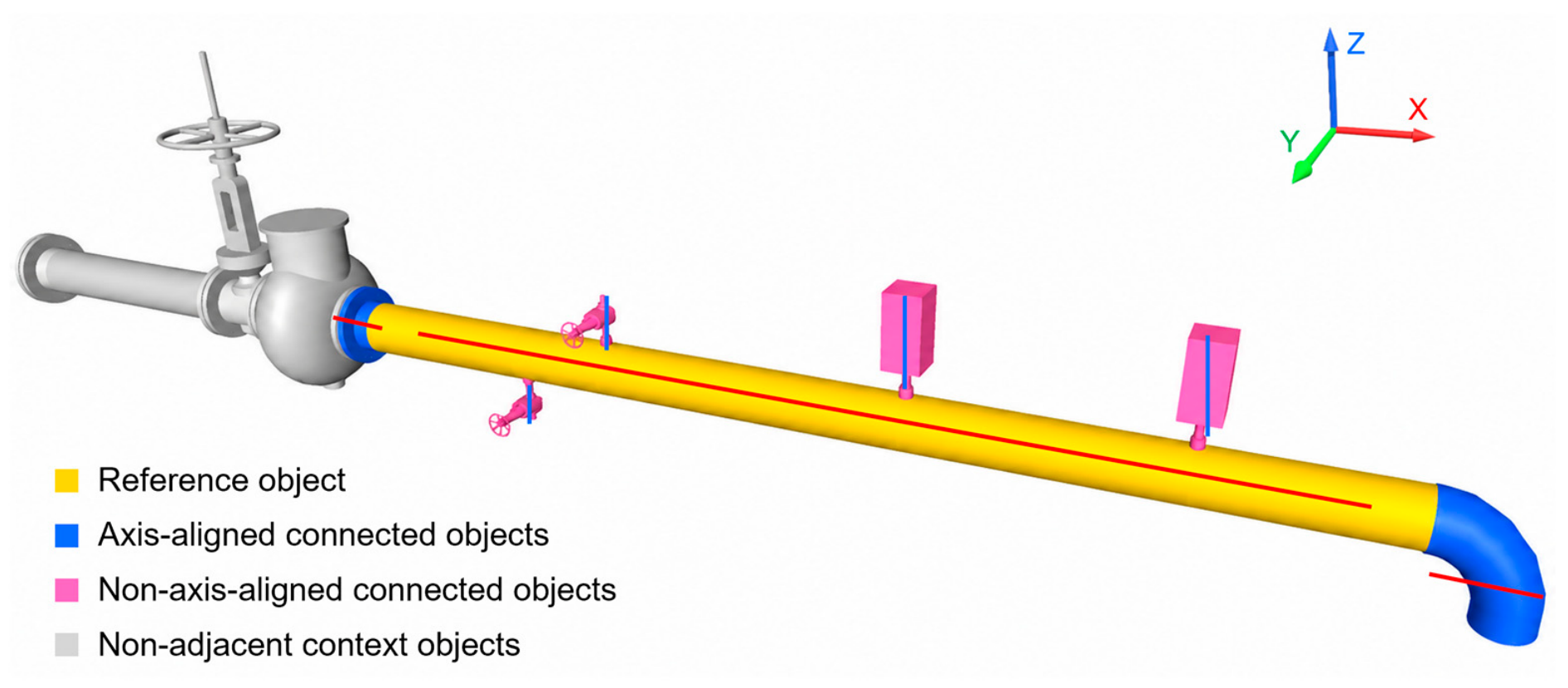
Figure 4 illustrates this axis-aware counting process using a pipe as the reference object. Although six objects are connected to the reference pipe in the validated connectivity graph, only the two objects aligned with the pipe’s main axis are counted toward its port usage. The four non-axis-aligned connections remain in the validated connectivity graph but are excluded from the pipe-side port count. The resulting direction-adjusted port count is then compared with the expected port count assigned to the corresponding component type. Objects whose direction-adjusted port count exceeds the expected value are flagged for manual review because one or more incident edges may be false positives. Objects with counts below the expected value are separately flagged as potentially incomplete or unresolved connections.
3.5. Connectivity-Based Installation Grouping
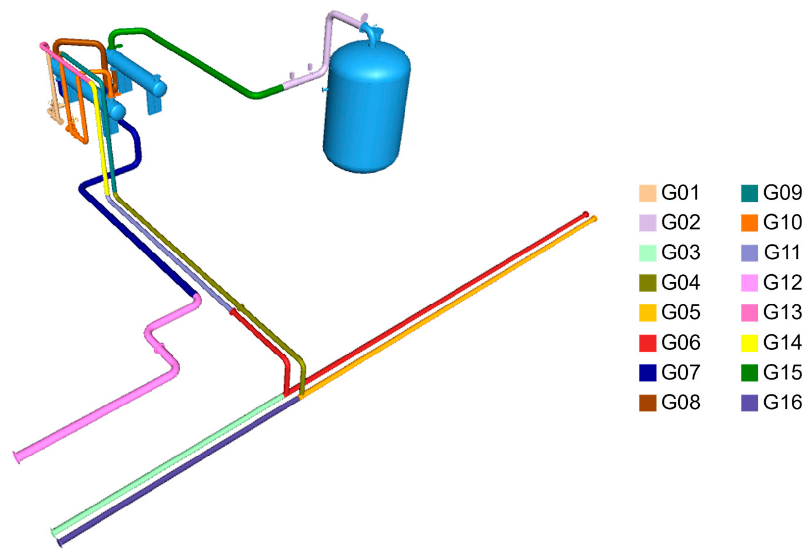
The validated connectivity graph is used to organize individual piping objects into installation groups. The overall grouping procedure is summarized in Algorithm 2 and consists of three main steps: initial grouping based on Pipeline and PipeRun properties, dimensional splitting, and connectivity-based merging.
First, initial object sets are established using each unique combination of Pipeline and PipeRun properties. Each initial set is then checked using the validated edges. If the objects do not form a single connected network, the disconnected portions are treated as separate initial segments. Next, the overall dimensions of each connected segment are evaluated to reflect practical constructability considerations. Based on a previous study that considered transportation-constrained mini-modules, a reference dimensional envelope of 80 ft × 13.5 ft × 13.5 ft was adopted for this case study [
27]. For each segment, a combined AABB is generated from its constituent objects, and the segment is considered dimensionally feasible when the combined AABB remains within this reference envelope. This envelope is treated as a configurable project-specific parameter rather than a universal limit and may be adjusted according to fabrication, transportation, lifting, site access, and installation requirements. Connected segments exceeding the dimensional limit are partitioned at existing object-to-object connections so that each resulting subsegment remains connected and satisfies the specified dimensional envelope. Preference is given to feasible partitions with fewer subsegments to avoid unnecessary fragmentation. Finally, the resulting feasible segments are examined for possible merging. Connected segments may be merged when at least one validated edge exists between them and the combined group remains within the dimensional limits. The merging process is repeated to reduce the number of resulting installation groups. The entire grouping procedure is applied only to piping objects.
| Algorithm 2. Connectivity-constrained installation group generation algorithm. |
| Input | |
| Output | |
as empty.
using each unique (Pipeline, PipeRun) combination.
do
6: end for
do
and obtain its ordered dimensions.
then
into feasible segments by removing validated edges.
11: end if
12: end for
14: for each do
and obtain its ordered dimensions.
then
and
18: end if
19: end for
20: Repeat feasible merges to reduce the number of resulting groups.
resulting groups.
|
3.6. Rule-Based Candidate Installation Sequencing
Once the installation groups are determined, a candidate installation sequence is generated based on predefined priority criteria. In this study, major equipment is assumed to have been installed and positioned before the associated piping is installed. Accordingly, for each piping network, an equipment-connected group is preferentially selected as the starting group (Equipment Connection Rule). When multiple equipment-connected candidates are available, the group associated with the larger-diameter main piping is given higher priority (Main-Line Priority Rule). Where candidate groups occupy vertically constrained installation spaces, the group at the higher elevation is preferentially installed to preserve installation access for the subsequent lower-level piping (Elevation Rule). If equivalent candidates remain after these criteria are applied, spatial continuity with the current work front and other installation conditions may be considered (Constructability Rule).
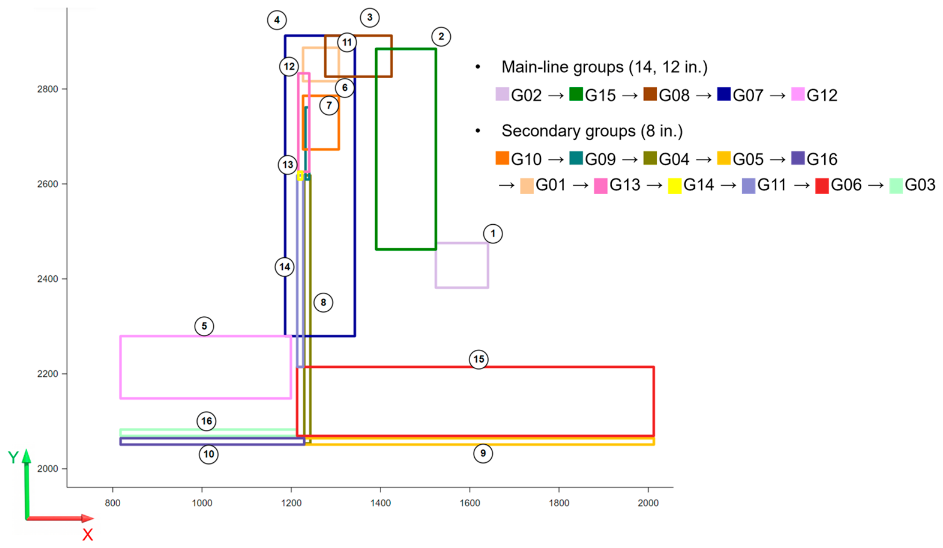
After a starting group is selected, subsequent groups are chosen from the uninstalled groups directly connected to the preceding group, thereby maintaining continuity along the same piping network. This process continues until all groups in the corresponding connected piping network have been sequenced. The procedure is then repeated for the remaining equipment-connected starting candidates. These priority criteria are intended to provide a candidate sequence for the case implementation and may be adjusted according to the piping system, construction conditions, and project-specific installation strategy.
6. Conclusions
The granularity gap between detailed BIM objects and construction schedules limits the direct use of BIM data for detailed installation planning and 4D BIM applications in industrial plant construction. To address this challenge, this study developed a framework for generating installation sequences from object-level BIM data of plant piping systems. The framework combines lightweight AABB-based geometry with piping-specific semantic information to establish object-level connectivity, organizes piping objects into dimensionally feasible installation groups based on Pipeline and PipeRun information, connectivity, and dimensional constraints, and subsequently applies predefined priority criteria to generate a candidate installation sequence. The framework was implemented as a custom Autodesk Navisworks add-in and evaluated using a process piping case model comprising 705 physical objects. The results demonstrate that the proposed filtering procedure can establish reliable object-level connectivity from AABB-based geometric relationships and piping-specific semantic rules. The grouping analysis showed that the initial Pipeline-PipeRun-based partitions were restructured through connectivity checking, dimensional splitting, and connectivity-constrained merging to form the final installation groups. Based on these groups, a candidate installation sequence was generated by prioritizing equipment-connected main-line groups and subsequently progressing along connected piping routes.
The main contribution of this study is the development of a BIM-based procedure that derives a candidate installation sequence from detailed plant piping objects without requiring predefined installation grouping or sequencing information in the BIM model. By integrating object-level connectivity inference, connectivity-based grouping, and rule-based sequencing within a single workflow, the proposed method provides an intermediate object-level planning structure for subsequent linkage with broader construction schedule activities. The generated installation groups and candidate sequence can therefore support subsequent detailed 4D BIM planning while reducing reliance on manual definition of installation logic during detailed scheduling. Despite these contributions, several limitations remain. The grouping process considered connectivity and dimensional constraints but did not account for other construction factors such as lifting capacity, fabrication requirements, material handling, or crew availability. In addition, residual false-positive relationships indicate that AABB-based connectivity inference may require additional geometric or semantic checks for densely arranged or irregularly shaped piping objects. Future research should incorporate additional constructability and resource constraints while further automating connectivity validation through approaches such as anomaly detection and higher-fidelity geometric representations, including oriented bounding boxes, to reduce reliance on manual review.