1. Introduction
University campuses bring routes, entrances, courtyards, squares, planted areas, and water edges into a compact pedestrian environment. In Tianjin’s hot-summer/cold-winter climate, outdoor design must provide protection from strong summer radiation without unnecessarily reducing winter solar access or increasing exposure to cold air movement [
1,
2,
3,
4,
5,
6]. The same spatial arrangement may therefore perform quite differently between seasons.
Outdoor thermal-comfort research has established that thermal response depends on climate, adaptation, and the physical setting [
7,
8,
9]. The Universal Thermal Climate Index (UTCI) and mean radiant temperature (Tmrt) are widely used to characterize these conditions [
10,
11,
12,
13,
14,
15,
16,
17,
18,
19,
20,
21], while studies of shade, canopy, enclosure, surface materials, sky exposure, and airflow have clarified many of the relevant physical pathways [
5,
6,
22,
23,
24,
25,
26,
27,
28,
29,
30,
31,
32,
33,
34,
35,
36]. A continuing difficulty is the interpretation of short field campaigns, particularly when direct measurements are combined with calculated indices, spatial proxies, and assumptions about how a place is used.
Campus and schoolyard studies have addressed thermal indices, seasonal comfort, landscape configuration, and mixed measurement–survey designs in a range of climates [
37,
38,
39,
40,
41,
42,
43,
44,
45,
46,
47,
48,
49]. Related studies examine outdoor activity, walkability, psychological adaptation, direct observation, campus walking, and movement trajectories [
50,
51,
52,
53,
54,
55]. Together, these studies show why thermal conditions, physical form, and patterns of use should be considered together, but they also show that each requires its own evidence. Plans and field notes can identify routes, entrances, adjacent programs, and places where people might stop. Actual pedestrian frequency, duration, and thermal perception require counts, behavior mapping, trajectories, or surveys. Without such observations, spatial descriptors can guide later fieldwork but cannot validate a measure of human exposure.
At a monitoring location, spatial form enters the analysis in two different ways. Vegetation, building mass, and enclosure can modify radiation, airflow, and near-ground temperature. Routes, entrances, and nearby programs describe the setting in which people may move or stay. Point-cloud data can define the first set of conditions, and plans can describe the second. Actual thermal exposure still depends on when people are present and how long they remain. Keeping these steps separate allows the physical evidence to be used without treating spatial form as observed behavior [
5,
6,
22,
23,
24,
25,
26,
27,
28,
29,
30,
31,
32,
33,
34,
35,
36,
50,
51,
52,
53,
54,
55].
UTCI and Tmrt answer related but different questions. UTCI combines air temperature, humidity, radiant temperature, and wind into an equivalent temperature, whereas Tmrt describes the radiant environment surrounding the body [
10,
11,
12,
13,
14,
15,
16,
17,
18,
19,
20,
21]. Reading them together is useful in heterogeneous outdoor spaces because a radiant advantage may be weakened or reversed by local air temperature and wind. Morphological measures such as canopy fraction or surrounding obstruction can suggest why radiant conditions differ, but they remain descriptions of form rather than direct measurements of shade, ventilation, or heat exchange [
5,
6,
22,
23,
24,
25,
26,
27,
28,
29,
30,
31,
32,
33,
34,
35,
36].
Spatial scale adds a second interpretive problem. A broad label such as courtyard, corridor, or wooded space can include positions with different crown structure, facade exposure, ground cover, and air paths. Values extracted within a single buffer may describe the selected sensor surroundings without representing every position assigned the same label. A credible site comparison therefore requires both a clearly defined analytical panel and a direct test of how the result changes when another same-setting position is used.
Short campaigns pose two distinct sampling problems. A span of a few days may capture an unusual weather episode, and a single sensor position may not represent every location carrying the same landscape label. Longer records address the temporal problem, whereas denser sampling addresses the spatial situation. When both are constrained, the episode must be placed in a weather distribution and the location choice tested directly. Timestamp-relative anomalies can then isolate simultaneous within-campus differences, provided that they are not interpreted as absolute comfort levels or as a seasonal climatology [
17,
18,
19,
20,
21,
37,
38,
39,
40,
41,
42,
43,
44,
45].
This study investigates relative thermal contrasts among twelve predefined open-space settings on one Tianjin university campus. The two monitored episodes are interpreted with four checks selected for a short and spatially heterogeneous campaign: consistency among the three calendar-day segments of each assembled 72 h table, comparison with the 2025 weather record, substitution of all same-setting candidates within the original 36-position sampling frame, and sensitivity to wind-height conversion. Point-cloud variables at 10, 25, and 50 m are used to define the morphology of all twelve locations. Route, entrance, program, and staying notes are retained separately as site context.
Accordingly, the study asks three questions: (1) Which locations departed most strongly and consistently from the contemporaneous twelve-location median in the monitored summer and winter periods? (2) Did those departures persist when alternative locations of the same predefined setting were substituted? (3) How can the point-cloud morphology of each location, read together with UTCI and Tmrt, guide targeted follow-up measurements and reversible design tests?
2. Materials and Methods
2.1. Study Area and Sampling Design
The study was carried out on Campus 1 of Tianjin University in Tianjin, China. The campus contains a compact mixture of teaching buildings, residences, dining and administrative facilities, paved courts and squares, tree-covered spaces, grass, and a water edge. These environments are connected by primary routes, secondary paths, building entrances, and short-stay spaces. The campus was treated as a single case in which contrasting outdoor settings could be compared under the same background weather.
The field dataset comprised 36 candidate positions assigned in advance to twelve microenvironment settings, with one to five candidates in each setting. One position from each setting formed the main analytical panel: open built-up space, discrete built-up space, high-albedo square, low-albedo functional pavement, hard courtyard, green courtyard, open axis, closed corridor, dense trees, open grass, sparse woods, and water edge. Open grass is uncommon on this campus, but the field description and campus plan confirmed P10 as the available open-grass location.
Table 1 lists the selected site code and the number of candidates represented by each setting.
All twelve selected locations had paired summer and winter entries in the archived analytical tables, a usable planar coordinate, complete point-cloud coverage, and sufficient map information for describing the surrounding campus setting. Before the morphology analysis, the projected coordinates of P03 (E = 514,630.626 m, N = 4,328,687.833 m) and the adjusted P10 field record (E = 514,552.436 m, N = 4,328,744.862 m) were checked against the campus plan and field records in UTM Zone 50N (EPSG:32650). The twelve locations form a purposive panel rather than a probability sample. Dependence on the retained location is examined by substituting all available same-setting candidates.
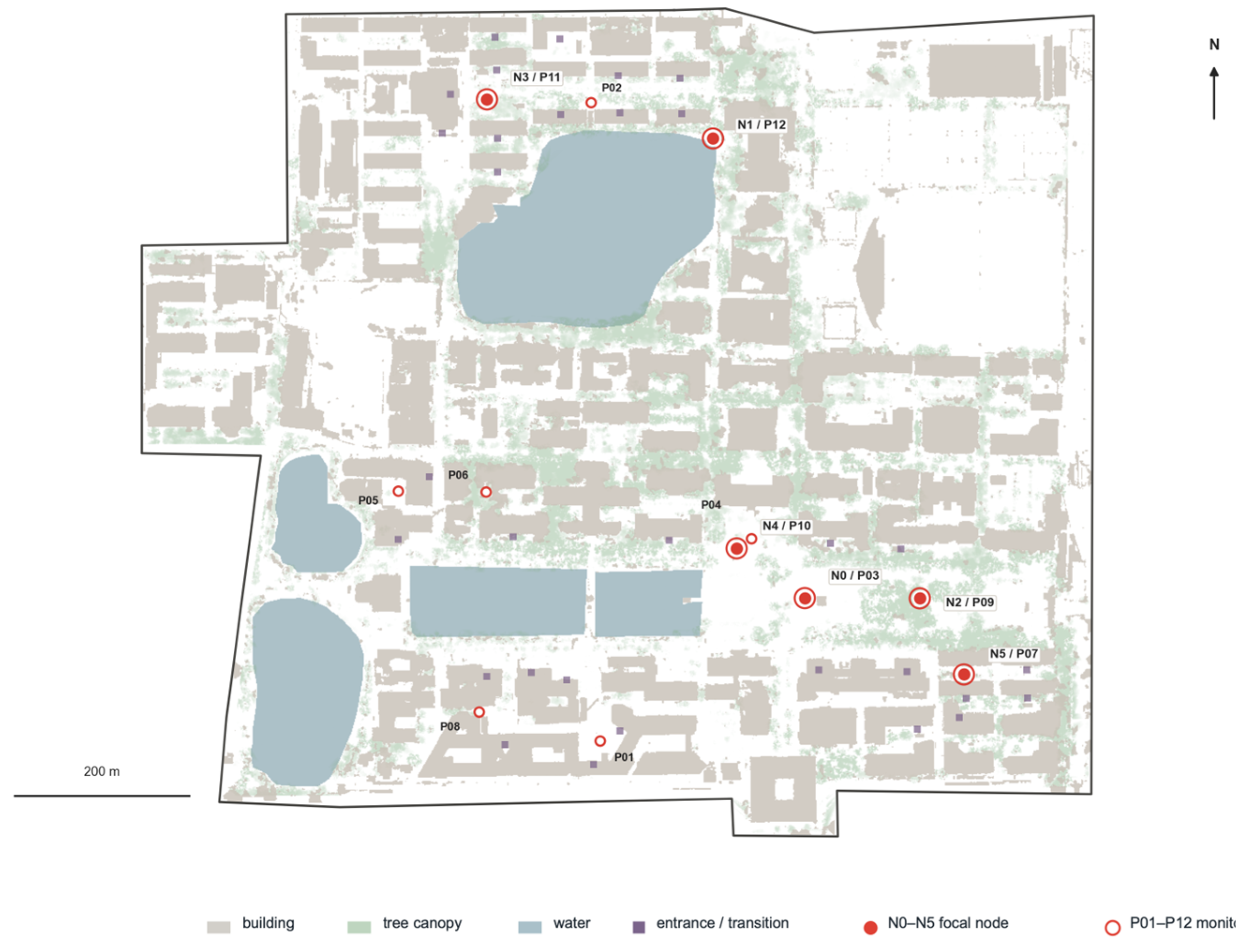
Figure 1 shows the case campus and the selected locations.
2.2. Field Campaigns and Instrument Deployment
The common analysis windows were 23–25 June 2025 and 16–18 December 2025, from 00:00 on the first day to 23:50 on the third day. Each window therefore contains 432 ten-minute timestamps. These windows define the compiled analytical table, which combines direct observations and calculated inputs rather than continuous full-variable measurements at all 36 positions. Archived winter logger deployments extended into 19 December, but records after 18 December 23:50 were not included in the main winter comparison. All field instruments were installed at 1.5 m above ground.
The field equipment consisted of three Kestrel 5400 LiNK heat-stress trackers (Nielsen-Kellerman Co., Boothwyn, PA, USA) and eight DS1923/iButton temperature–humidity loggers (Analog Devices, Inc., Wilmington, MA, USA). One Kestrel served as a fixed reference, and two were moved among field positions. The DS1923 loggers were housed in naturally ventilated radiation shields. Where a Kestrel was present, it directly recorded air temperature (Ta), relative humidity (RH), local wind speed, equivalent globe temperature, and device heat-stress outputs. Where a shielded DS1923 was present, Ta and RH were direct measurements. Tmrt and UTCI were calculated variables.
Table 2 summarizes these roles.
The recovered deployment archive documents six summer logger records (archival codes P1–P6) from 23 June 09:54 to 25 June 10:19, with 582 records per logger; P3 contained 108 missing Ta/RH entries. In winter, the eight DS1923 loggers were redeployed across three successive six-position blocks (A1–A6, B1–B6, and C1–C6), producing 18 position-level deployment records with 136–146 records per position. The blocks represent different positions observed successively and not 18 physical instruments or the same six positions repeated on three days. Complete Kestrel sessions recoverable for the channel audit comprised 451 summer and 166 winter records.
Supplementary Tables S2b and S2c provide the point coefficients and deployment-level coverage.
Manufacturer specifications are ±0.5 °C for Kestrel air temperature, ±2% for RH, and ±1.4 °C for equivalent globe temperature. The stated DS1923 accuracy is better than ±0.5 °C between −10 and 65 °C after software correction, with an RH accuracy of ±5% [
56,
57]. A campaign-specific co-location calibration for all eleven devices was not retained. As a channel check, outdoor wet-bulb globe temperature was recalculated for identifiable complete Kestrel sessions and closely matched the device output in summer (
n = 451, r = 0.996, RMSE = 0.17 °C) and winter (
n = 166, r = 0.9998, RMSE = 0.04 °C). The channel check covers the identifiable Kestrel sessions; non-Kestrel intervals retain the archived processed values.
2.3. Data Assembly and Thermal-Index Calculation
Ta and RH are identified as measured when a Kestrel or shielded DS1923 record was available at that location and interval. Wind and equivalent globe temperature (Tg) are identified as measured only during Kestrel deployment. The complete 36-position tables also contain values for intervals without full Kestrel coverage. In those cells, wind is a calculated input derived from the archived background series and point coefficients, and Tg is the retained processed estimate. The archived files do not retain a cell-level source flag. Measured-versus-calculated coverage is therefore reported at the variable and deployment levels in
Tables S2a–S2c, together with the recovered coefficients.
All timestamps were handled in China Standard Time (UTC+8). The hourly background series was linearly interpolated to the 10 min grid before the archived location coefficients were applied. Records were sorted by site and time, with temperature retained in degrees Celsius, RH in percent, and wind in m s−1. Each seasonal Campus-1 table contains 15,552 rows (36 positions × 432 timestamps), without duplicate position–timestamp combinations or blank primary fields. The selected twelve-position panel contains 5184 aligned rows per season. This completeness describes the assembled table, not simultaneous full-channel instrument coverage.
For cells without direct Kestrel wind measurements, the recovered summer relation is WS = WSBG × 0.630 × ks, where WSBG is the interpolated background wind, and ks is the archived position coefficient. A three-point rolling median was then applied, and values below 0.25 m s
−1 were set to 0.25 m s
−1. The winter proxy is WS = WSBG × kw. The full ks and kw register for A1–A36 is reported in
Table S2b. Winter Kestrel wind recorded in km h
−1 was divided by 3.6. These proxy series are not described as measured local wind.
The Kestrel 5400 LiNK contains a 25 mm black-coated copper globe and exports a globe-temperature value converted by the manufacturer to the equivalent response of a standard 150 mm globe [
56]. During complete Kestrel sessions, this equivalent Tg is a direct device output. Outside those sessions, the compiled table retains Tg_est_C as a processed estimate. The archived non-Kestrel Tg cells retain the processed estimates used in the original analysis; the dated generating equation and cell-level source register were not retained. Independent regeneration is available only for the retained Kestrel sessions. Tmrt was calculated from the retained Tg, Ta, and local wind v using the ISO 7726 globe heat-balance expression [
58]:
where D = 0.150 m, and ε = 0.95. UTCI was calculated from Ta, RH, Tmrt, and wind, with the polynomial implementation in pythermalcomfort 2.10.0 [
59]. The UTCI implementation was independently rerun from the retained analytical fields and reproduced the table values to the reported precision. The baseline comparison uses the local 1.5 m wind field, constrained to the UTCI input range of 0.5–17 m s
−1. Because a morphology-specific vertical profile was not measured, conversion to 10 m is treated as a sensitivity analysis rather than as a correction; Equation (2) uses α = 0.14, 0.22, and 0.33 to bracket open, rough/suburban, and urban profiles [
60,
61].
The summer comparison was restricted to peak-solar conditions, defined by a clear-sky solar proxy of at least 650 W m−2 and a solar zenith angle no greater than 45°. In the Campus-1 data, this selected 09:00–15:30 and 120 records per location. The winter comparison used a solar proxy above 50 W m−2 and a solar zenith angle below 90°, selecting 07:50–16:20 and 156 records per location.
To remove the common weather signal at each timestamp, the median of the twelve selected locations was used as the panel reference. For X representing UTCI or Tmrt, the location anomaly was calculated as
Seasonal location estimates were the medians of the ten-minute anomalies within the summer and winter analysis windows. Positive values indicate a warmer condition than that of the contemporaneous campus panel, and negative values show a cooler condition. Continuous values are reported throughout. A ±0.25 °C band was used when a near-neutral description was needed, with ±0.50 and ±1.00 °C tested as alternative bands.
The timestamp median was preferred to the arithmetic mean because it is less affected by a single large site departure. The same twelve-location panel was used at every timestamp, and the seasonal median was calculated only after the timestamp-specific subtraction. The resulting anomalies are relative spatial contrasts within the case campus. A value near zero means that the value is close to the contemporaneous panel median; it is not a thermal-comfort threshold or a neutral vote from campus users.
2.4. Weather Context and Robustness Analyses
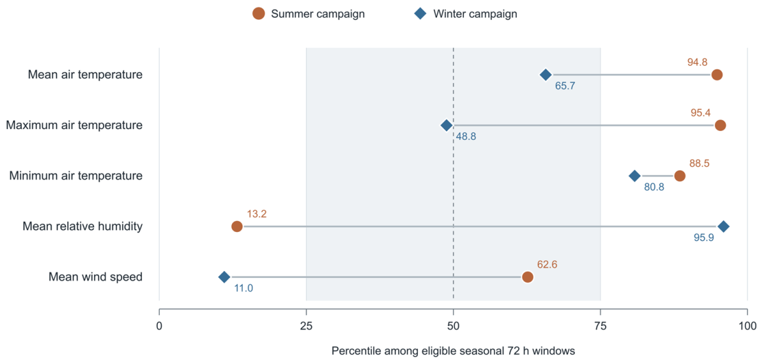
The meteorological setting of each campaign was assessed with an archived hourly record for World Meteorological Organization (WMO) station 54517 (Tianjin urban; 39.0747° N, 117.2061° E), approximately 4.98 km from the campus. The file contains 8760 hourly observations for 2025. For summer, the three-day campaign was compared with every complete, daily-starting 72 h window in June–August; the winter comparison used windows for January–February and December. Eligible windows required complete air-temperature, RH, wind-speed, and precipitation records for all 72 h. Campaign means, minima, maxima, and percentile ranks were calculated against the corresponding seasonal distribution. This comparison positions the monitored episodes within the 2025 record rather than treating them as long-term seasonal normals.
For each weather variable, the percentile rank equals 100 times the proportion of eligible windows whose value was no greater than the campaign value. Precipitation was reported directly. These ranks describe how the two monitored episodes sit within the available 2025 seasonal windows.
Table 3 reports the campaign metrics, and
Figure 2 displays their percentile positions.
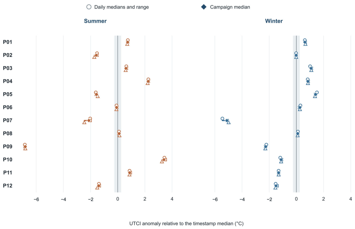
Temporal consistency was evaluated by splitting each assembled 72 h table into three calendar-day segments and calculating a daily median anomaly for every location. The ten-minute rows were not treated as independent replicates, and the three segments are not presented as three independent deployments at each location. With only three descriptive segments, formal significance testing would add little value; the analysis therefore reports direction and range.
The location-selection sensitivity analysis used all 36 positions in the assembled sampling frame. Each candidate replaced the selected position for its setting, while the other eleven locations remained fixed; UTCI, the timestamp-specific panel median, and the seasonal anomaly were then recalculated. The selected value was compared with the candidate median and full range. This procedure tests dependence on analytical location choice within the compiled table. It is not an independent validation sample and does not increase the number of directly instrumented stations.
The three wind-height conversions defined in
Section 2.3 provide a separate processing check. Tmrt was held at the value calculated using local wind at instrument height because the globe heat-balance equation uses wind at that height; UTCI alone was recalculated with the alternative v10 inputs. The daily segments, neutral bands, candidate substitutions, and wind profiles therefore examine temporal patterning within the assembled table, threshold choice, location-selection dependence, and wind-processing sensitivity. None of these substitute for a fully synchronized multi-station campaign.
2.5. Point-Cloud Morphology and Site Context
Campus morphology was derived from a 528,360,229-point LAS 1.4 dataset (point format 7) referenced to EPSG:32650 and recorded as having been processed in LiDAR360. The classified data included ground, building (class 6), and vegetation (classes 4–5) returns. Available 1 m products included a digital elevation model, a normalized digital surface model (nDSM), a canopy-height model, and a building-height raster. The point-return metrics and the nDSM metrics were kept distinct in the analysis.
The canopy proxy was calculated as the share of all returns assigned to vegetation at least 2 m above ground, and the building proxy as the share of returns assigned to class 6. The 95th-percentile heights of canopy and building returns were retained as supplementary descriptors. High obstruction was calculated independently as the fraction of valid 1 m nDSM cells at least 2 m above ground, and openness as one minus that fraction. The water proxy is the share of class-9 returns and is reported for P12. All ratios range from 0 to 1. Because point-return proportions depend on scan geometry and return density, the canopy and building variables are treated as morphology proxies rather than as plan-area cover fractions. None of these variables is a direct measure of sky-view factor, shade duration, radiation, or airflow.
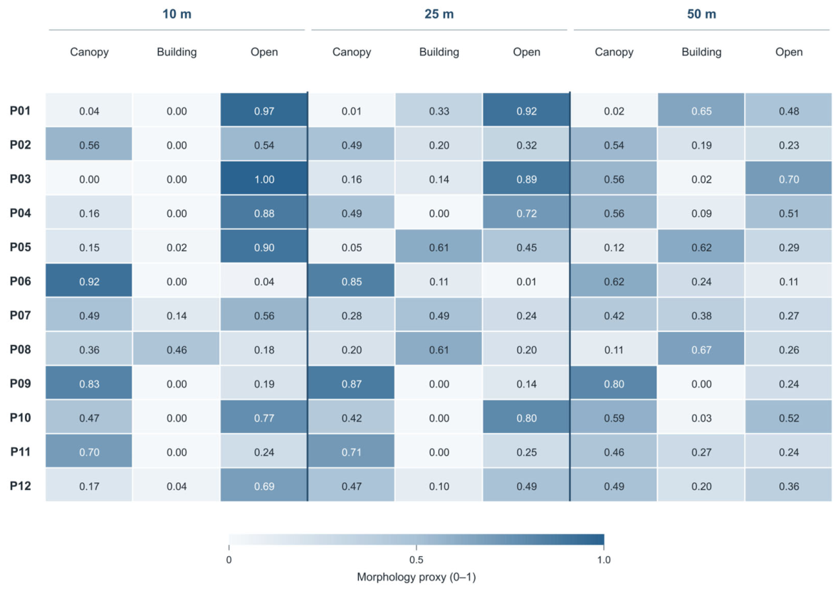
The variables were calculated within 10, 25, and 50 m buffers around every selected coordinate. The 10 m buffer describes the immediate sensor surroundings, the 25 m buffer the local setting, and the 50 m buffer the wider neighborhood. Changes across the three buffers were used to identify where a point lay in an open core, near a building or canopy edge, or within a consistently obstructed setting.
Figure 3 presents this multiscale comparison for all twelve locations; the 25 m values are retained in the main numerical table, and the complete three-scale values are reported in
Supplementary Table S5.
Four map-based notes were recorded separately: relation to a campus route, nearby program, relation to an entrance, and the physical provision for waiting or staying. These notes describe site context only. They are not measurements of pedestrian presence or dwell time, are not summed, and do not enter the thermal analysis or a priority ranking. Their purpose is to specify where subsequent counts, trajectories, dwell observations, or short surveys would be useful.
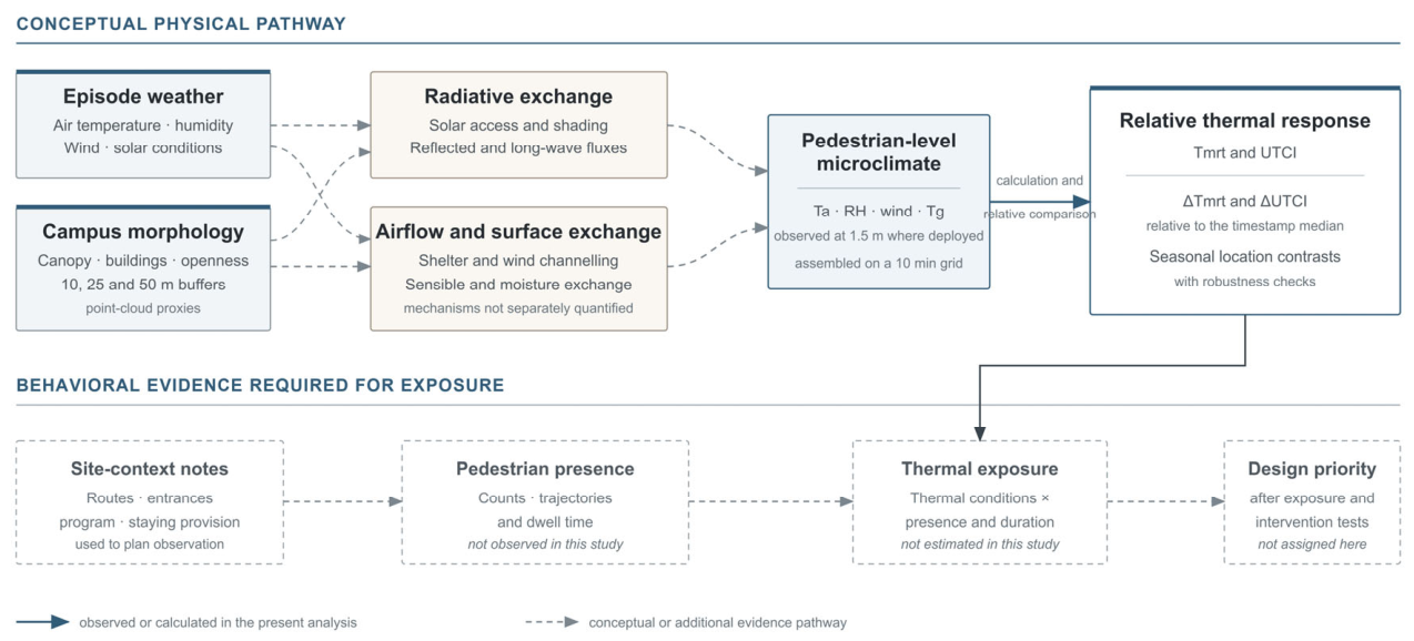
Figure 4 summarizes the conceptual pathways used to interpret the analysis. Episode weather and multiscale campus morphology may modify radiative exchange, airflow, and surface heat and moisture exchange, which together shape the pedestrian-level variables used to calculate Tmrt and UTCI. These mechanisms were not separately quantified, so the point-cloud variables are used to interpret rather than causally partition the observed thermal contrasts. Estimating thermal exposure would additionally require synchronized observations of pedestrian presence and dwell time; design priority would require those exposure data, along with intervention testing.
3. Results
3.1. Meteorological Context of the Two Campaigns
Among the 87 eligible summer windows, the monitored period lay near the hot end of the 2025 distribution. Mean air temperature was 31.98 °C (percentile rank, 94.8), the maximum was 38.5 °C (95.4), and the minimum was 26.3 °C (88.5). Mean RH was comparatively low at 41.69% (13.2), mean wind speed was 2.20 m s−1 (62.6), and no rainfall was recorded. Only 27.6% of eligible summer windows were rain-free.
Relative to the 86 eligible winter windows, the monitored episode was mild, humid, and calm. Mean air temperature was 2.31 °C (percentile rank, 65.7), with a maximum of 7.0 °C (48.8) and a minimum of −2.1 °C (80.8). Mean RH had a percentile rank of 95.9 (64.47%), whereas mean wind speed ranked at 11.0 (1.49 m s−1); precipitation was 0 mm. We interpret the two campaigns as a hot, dry summer episode and a mild, humid, low-wind winter episode.
3.2. Relative Thermal Contrasts Among the Twelve Locations
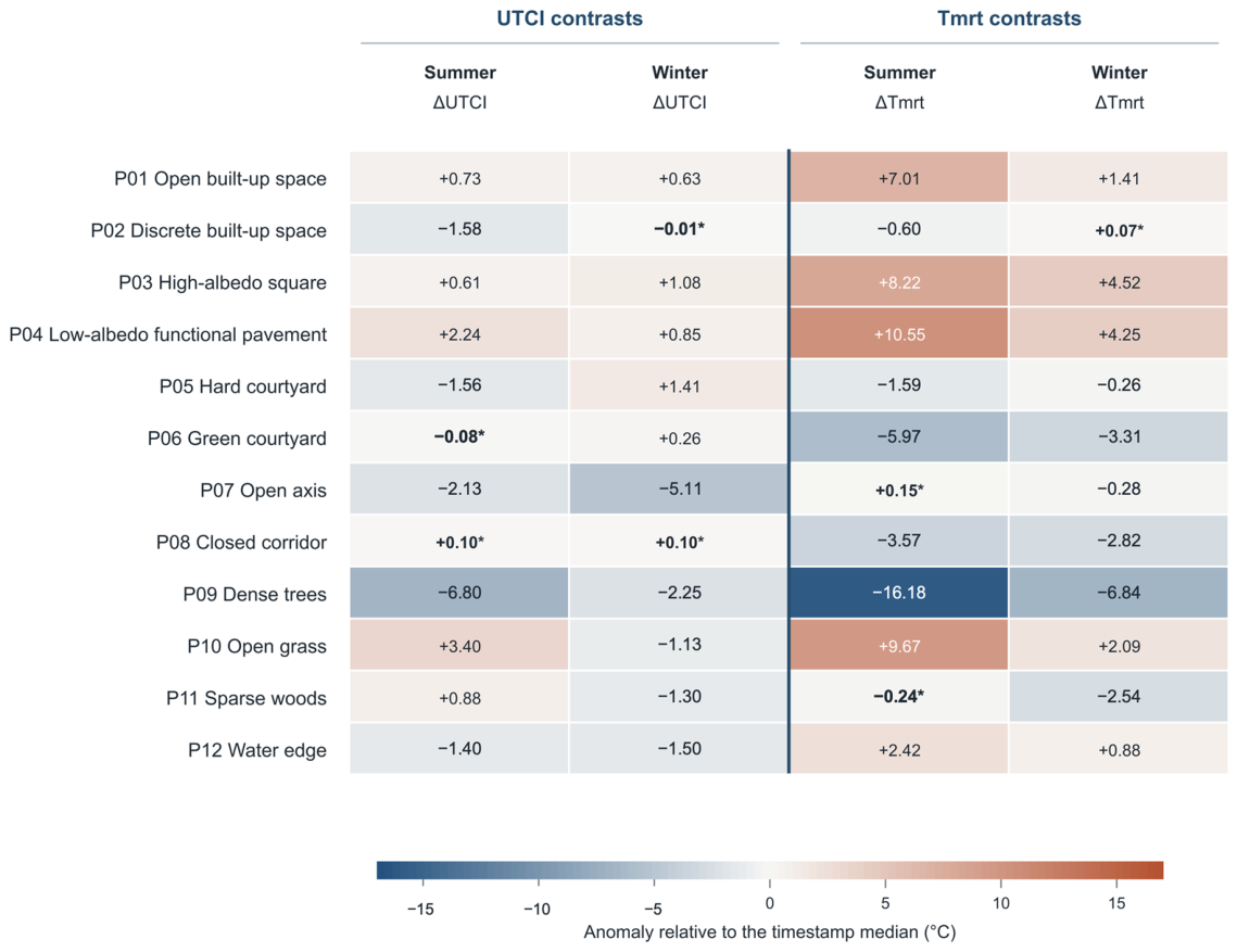
During the summer peak-solar period, dense trees at P09 showed the largest negative anomaly (ΔUTCI = −6.80 °C). The open axis P07 (−2.13 °C), discrete built-up space P02 (−1.58 °C), hard courtyard P05 (−1.56 °C), and water edge P12 (−1.40 °C) were also cooler than the timestamp median. Open grass P10 (+3.40 °C) and low-albedo functional pavement P04 (+2.24 °C) had the largest positive anomalies. P06 (−0.08 °C) and P08 (+0.10 °C) fell within the near-neutral interval.
In the winter daytime period, P07 had the largest negative anomaly (−5.11 °C), followed by P09 (−2.25 °C), P12 (−1.50 °C), P11 (−1.30 °C), and P10 (−1.13 °C). P05 (+1.41 °C), P03 (+1.08 °C), P04 (+0.85 °C), and P01 (+0.63 °C) were warmer than the contemporaneous median. P02 (−0.01 °C) and P08 (+0.10 °C) were near-neutral.
Using the ±0.25 °C band, seven locations remained in the same category in both campaigns. P01, P03, and P04 were warmer than the panel median in summer and winter; P07, P09, and P12 were cooler in both; and P08 remained near-neutral. P02 changed from cooler to near-neutral, P05 from cooler to warmer, and P06 from near-neutral to warmer. P10 and P11 reversed from warmer in summer to cooler in winter. Among locations whose anomalies changed sign, the largest seasonal change occurred at P10 (+3.40 to −1.13 °C), followed by P05 (−1.56 to +1.41 °C).
The radiant-temperature contrasts were wider in summer than in winter. Summer ΔTmrt ranged from −16.18 °C at P09 to +10.55 °C at P04, a span of 26.73 °C; P03 and P10 also exceeded +8 °C. The winter range extended from −6.84 °C at P09 to +4.52 °C at P03. P04 remained strongly positive (+4.25 °C), while P06, P08, and P11 had negative winter ΔTmrt. The relative UTCI and Tmrt patterns agreed at some locations but diverged at others, indicating that radiation alone did not account for all site contrasts.
The main conclusions were also insensitive to modest changes in the near-neutral band. Increasing the band from ±0.25 to ±0.50 °C left the summer category counts unchanged and moved only one additional winter value into the near-neutral group. At ±1.00 °C, five locations in each season were near-neutral, but P07 and P09 remained cooler in both campaigns, and P10 remained warmer in summer and cooler in winter.
Three patterns warranted closer examination. P09 was cooler in both campaigns, P07 showed a pronounced winter deficit, and P10 reversed from a positive summer anomaly to a negative winter anomaly. P11 showed the same reversal at the selected point, although the second sparse-woods candidate did not reproduce the summer direction.
Figure 5 and
Table 4 summarize the corresponding location-level values and categories.
3.3. Temporal and Location-Selection Robustness
Within the assembled 72 h tables, all 24 location–season estimates retained the same sign in each calendar-day segment. Introducing the ±0.25 °C near-neutral band changed the classifications of P02 in winter, P06 in summer, and P08 in both seasons relative to a zero-width band. The repetition indicates temporal consistency within each assembled episode; the three values are calendar-day segments of the same compiled series.
Daily-segment variation was modest relative to the strongest spatial contrasts. Summer ΔUTCI at P09 ranged from −6.83 to −6.80 °C, P10 from +3.25 to +3.50 °C, and P07 from −2.46 to −2.02 °C; all other summer ranges were 0.25 °C or narrower. In winter, P07 remained the most negative location in every segment (−5.44 to −4.98 °C), and the ranges at the other eleven locations did not exceed 0.15 °C.
Figure 6 displays these descriptive ranges.
Candidate substitution produced the same directional category as that of the selected location in 10 of 12 settings in summer and 11 of 12 in winter. All open-axis and dense-tree candidates were cooler in the relevant periods, and both open-grass candidates were warmer in summer and cooler in winter. The two sparse-woods candidates differed in summer, while P12 had no alternative water-edge candidate. Complete candidate ranges are reported in
Supplementary Table S8 and Figure S3.
The disagreements were concentrated in small or spatially variable contrasts. In summer, selected P06 was near-neutral (−0.08 °C), whereas the three green-courtyard candidates had a cooler median and ranged from −2.83 to −0.08 °C. Selected P11 was warmer (+0.88 °C), but the second sparse-woods candidate was cooler (−2.19 °C). In winter, selected P02 was near-neutral (−0.01 °C), while its four candidates ranged from −0.71 to −0.01 °C and had a cooler median. P08 remained near-neutral at the selected and median values, although its candidate ranges crossed zero in both seasons. These ranges are used to distinguish a stable selected-site result from a claim regarding an entire setting.
Wind-height conversion altered anomaly magnitudes more strongly in winter than in summer, but the principal P07, P09, and P10 categories remained unchanged. Across α = 0.14–0.33, summer ΔUTCI ranged from −2.83 to −2.53 °C at P07, −6.76 to −6.55 °C at P09, and +2.88 to +3.16 °C at P10. The corresponding winter ranges were −8.95 to −6.75, −1.74 to −0.59, and −2.68 to −1.90 °C. Rank correlations with the local-wind results were 0.958–0.979 in summer and 0.825–0.881 in winter; 10–12 summer locations and 9–11 winter locations retained their baseline category, depending on the profile assumption.
3.4. Point-Cloud Definition and Thermal Context of the Twelve Locations
Figure 3 and
Table 5 define the twelve monitoring locations from the point-cloud data. The three buffers distinguish the immediate sensor surroundings from the local setting and the wider neighborhood. The predefined labels remain useful for sampling, but they do not replace the measured morphology at each coordinate.
P01 had an open 10 m core (openness 0.97) and remained open at 25 m (0.92), although the 50 m buffer included substantial building influence. P02 was a mixed vegetation–building setting, with low openness at 25 and 50 m (0.32 and 0.23). P03 was fully open at 10 m and largely open at 25 m; vegetation entered mainly at 50 m, where the canopy proxy rose to 0.56. P04 also had an open core, but its canopy proxy increased from 0.16 at 10 m to 0.49 at 25 m and 0.56 at 50 m. At P05, openness fell from 0.90 at 10 m to 0.45 at 25 m and 0.29 at 50 m as the surrounding building proxy increased.
The central group was more enclosed. P06 remained canopy-dominated at all scales (0.92, 0.85, and 0.62), with openness no higher than 0.11. P07 had a moderately open 10 m core (0.56), but openness fell to 0.24–0.27 in the larger buffers as building influence increased. P08 was building-dominated at every scale: the building proxy rose from 0.46 at 10 m to 0.61 at 25 m and 0.67 at 50 m, while openness remained between 0.18 and 0.26.
P09 differed from the other wooded locations because its canopy proxy remained high across all three buffers (0.80–0.87), and building returns were negligible. P10 was open at 10 and 25 m (0.77 and 0.80), with little building influence; the 50 m buffer contained more vegetation. P11 was locally wooded, with canopy proxies of 0.70 and 0.71 at 10 and 25 m, but the 50 m buffer included a building proxy of 0.27. At P12, water returns accounted for 0.40 of the 10 m point returns and declined to 0.16 and 0.10 at the larger scales, while vegetation and building influence increased.
These distinctions help to interpret, but do not by themselves explain, the thermal contrasts. The persistent canopy at P09 accompanied the largest negative summer ΔTmrt and ΔUTCI. P06 was even more obstructed locally but had a near-neutral summer ΔUTCI, and P11 did not reproduce the P09 radiant response. The paved cores at P03 and P04 exhibited a positive summer ΔTmrt, whereas the large winter UTCI deficit at P07 occurred with little radiant departure. The point-cloud data therefore narrow the physical setting of each result without assigning a single thermal effect to a broad landscape label.
4. Discussion
4.1. Interpreting the Seasonal Contrasts
The principal finding is not a single year-round ranking of campus spaces, but a set of seasonal contrasts with different likely drivers. Pairing ΔUTCI with ΔTmrt helps separate cases dominated by radiant conditions from those in which air temperature or wind deserves closer attention. At P09, the two anomalies moved in the same direction, whereas the large winter UTCI deficit at P07 occurred with little radiant departure. The comparison does not partition causal contributions, but it identifies the variable that should be measured more intensively in a confirmatory campaign.
The background weather comparison is important to that interpretation. Strong heat and the absence of rain characterized the summer episode, while the winter episode combined high humidity with relatively low station wind. These conditions may accentuate different parts of the outdoor heat balance. They also limit direct seasonal extrapolation: the summer values describe a hot, dry event, and the winter values a mild, calm event. Timestamp-relative anomalies remove much of the common weather signal, but they do not show how the same locations would respond during a cooler summer spell, a windy cold wave, or another year.
At P09, both dense-tree candidates retained a negative summer ΔUTCI, and the selected location also had a strongly negative ΔTmrt. Winter ΔTmrt remained negative, indicating lower radiant gain during the mild winter episode. This pattern agrees with the results for established canopy and shade mechanisms [
5,
6,
22,
23,
24,
25,
26,
27,
28]. Direct measurements of crown transmissivity, time-varying shade, and under-canopy airflow would be needed to determine the contribution of each mechanism at this location.
At 25 m, P09 and P06 had similar canopy proxies (0.87 and 0.85), but their summer ΔUTCI differed by 6.72 °C. Their multiscale structure was not identical: the canopy proxy at P09 remained between 0.80 and 0.87 from 10 to 50 m, whereas at P06, it declined from 0.92 to 0.62. P11 was locally wooded at 10 and 25 m, but its canopy proxy fell to 0.46, and its building proxy rose to 0.27 at 50 m. These differences show why the sensor surroundings should not be inferred from a landscape label alone. Crown transmissivity, leaf density, ground moisture, and under-canopy ventilation remain unmeasured and offer testable explanations for the contrasting thermal responses.
P07 and P12 illustrate a different diagnostic problem. The winter deficit at P07 was large and stable across the open-axis candidates, although its ΔTmrt was only −0.28 °C. P12 combined a negative ΔUTCI with a positive ΔTmrt. Both patterns point toward a stronger role for local wind and air-temperature structure than for radiation alone, making synchronized anemometry, Ta, and globe-temperature measurements the appropriate next testing scenario.
The seasonal reversals at P10 and P05 likewise cannot be read from radiation alone. P10 retained a positive ΔTmrt in both campaigns (+9.67 and +2.09 °C), while ΔUTCI changed from +3.40 to −1.13 °C. At P05, ΔUTCI shifted from −1.56 to +1.41 °C although ΔTmrt remained slightly negative. Simultaneous measurements of local air temperature, wind, humidity, and radiation would allow the individual contributions to be separated in a subsequent campaign.
4.2. Relation to Campus Microclimate Research
The summer response at P09 and the positive radiant anomalies at the paved sites agree in direction with recent studies of campus canopy, shade, and surface exposure [
7,
8,
27,
39,
44]. The present analysis adds a set of checks tailored to short field campaigns: the weather distribution establishes the conditions sampled, calendar-day segment medians describe within-episode consistency, candidate substitution tests dependence on location choice, and wind conversion tests a key processing assumption. Their practical value lies in showing which contrasts remain credible enough to justify a more focused campaign.
Earlier campus studies provide useful comparisons of response direction. In a four-location field study, the shaded path received the highest share of “comfortable” votes, and UTCI performed consistently across the tested spaces [
37]. A campus-courtyard simulation found summer benefits from tree–lawn combinations and showed that high-reflectivity concrete could lower air and surface temperatures while increasing PET through additional radiant exposure [
39]. The positive ΔTmrt at P03 and P04 follows the same physical direction, although differences in climate, index, intervention, and study design preclude a direct comparison of effect size.
The comparison among P09, P06, and P11 also cautions against transferring an effect size from a landscape label alone. Similar local canopy-return proxies can occur within different wider settings, and neither the return proxy nor the obstruction fraction records crown transmissivity, solar penetration, soil condition, or ventilation. Cross-study agreement is therefore more defensible at the level of physical direction—such as shade reducing radiant load—than at the level of a universal temperature reduction.
Studies combining monitoring with questionnaires or direct observation demonstrate what is required to connect thermal conditions with campus use [
45,
46,
47,
48,
49]. Work on a cold-region campus in Xi’an linked measurements and questionnaires with activity logs [
46], while a study of ten campus green spaces examined 982 questionnaires and 3864 activity records [
49]. Such designs distinguish a heavily used route from a space that merely appears accessible on a plan. In the present study, the route, entrance, program, and staying notes serve only to select sites and observation periods for that next stage.
Separating site context from observed exposure changes how the thermal results can be used. A route or entrance note can help determine where and when pedestrian observation should be conducted, but it should not be combined with the thermal anomaly to determine a user priority. A thermally extreme space that is rarely occupied and a heavily used space with a small thermal departure pose different management questions. Simultaneous counts, dwell observations, or short surveys are needed before thermal performance and actual campus use are considered together.
4.3. Implications for Campus Design and Follow-Up
For campus practice, the results support a staged approach. Repeat measurements should first confirm the contrasts under comparable weather. The next campaign can then target the process suggested by the paired ΔUTCI–ΔTmrt pattern—radiation, wind, air temperature, or surface condition—while recording pedestrian movement and dwell time during the same periods. Temporary interventions or calibrated simulations can be introduced once the local process has been identified, with both summer and winter monitoring used to check the trade-off.
The required tests differ by location. At P09, winter shortwave exposure and crown transmissivity should be measured before selective thinning or seasonal pruning is considered. Temporary shade at P03 and P04 can be evaluated with globe temperature and pavement-surface measurements. P07 requires fixed local anemometry and Ta monitoring before a wind screen is sized or positioned. At P10, a removable summer shade structure would test the radiant penalty without permanently enclosing the campus’s limited open-grass area. Each trial should include an untreated reference period and simultaneous records of use or dwell time.
A broader validation program would repeat the synchronized thermal and pedestrian observations on additional campuses and under different weather conditions. Once the field mechanisms are established, calibrated computational fluid dynamics or related simulations could be used to compare reversible interventions and longer climate scenarios [
62,
63,
64,
65]. Automated GIS extraction may help to identify candidate sites, but the intervention model should remain tied to field observations.
On the case campus, P09 is suited to a test of improved winter solar access that preserves summer canopy performance. P03 and P04 warrant trials of adjustable or deciduous shade. P07 should receive wind-focused monitoring before a shelter or enclosure is proposed. P10 provides a site-specific opportunity to examine summer solar exposure and winter cooling in the campus’s limited open-grass setting. Additional water-edge locations and direct wind measurements are needed before the P12 response can be extended beyond that point.
P07, P09, and P10 are the strongest candidates for follow-up because their categories were unchanged across calendar-day segments, candidate substitutions, and every wind-height scenario. P08 and P11 require more spatial replication before a setting-level intervention is designed, since their candidate ranges crossed categories. P12 can support a location-specific wind and radiation study, but it is the only water-edge candidate. This ordering concerns the strength of the thermal evidence and does not rank the importance of the spaces to campus users.
4.4. Study Scope and Limitations
The evidence comes from one campus, twelve selected analytical locations, and two 72 h episodes in 2025. Three Kestrel units and eight shielded loggers supplied direct observations, but the deployment was not equivalent to simultaneous full-channel monitoring at 12 or 36 positions. The complete panel also uses background-weather inputs, archived point coefficients, wind proxies, and processed Tg estimates for uncovered cells. The wind relations and all recovered coefficients are reported in
Section 2.3 and
Supplementary Tables S2b and S2c, but the original cell-level device register and the dated non-Kestrel Tg equation were not preserved. Accordingly, the reported Tmrt and UTCI values are processed within-campus contrasts. The interpretation emphasizes contrasts that retain their direction under the location and wind checks.
These checks address specific, limited questions. Calendar-day segments describe temporal consistency within each assembled episode; candidate substitution tests dependence on the retained analytical position; wind scenarios show the effect of an unmeasured vertical profile; and the weather comparison identifies the type of episode sampled. The summer event was hot and rain-free within the 2025 record, whereas the winter event was mild, humid, and calm. These analyses do not establish climatological representativeness, independent replication, behavioral exposure, or causal effects of morphology. A future campaign should keep fixed full-channel instruments at the focal locations and preserve a cell-level provenance flag from ingestion through index calculation.
5. Conclusions
This exploratory case study identified marked contrasts among twelve analytical locations on one Tianjin university campus during a hot, rain-free summer episode and a mild, humid, low-wind winter episode. Within the assembled tables, P09 had the largest negative summer ΔUTCI and a lower winter Tmrt, P07 had the largest winter ΔUTCI deficit despite a small ΔTmrt anomaly, and P10 showed a change from warmer than the panel median in summer to cooler in winter. These location-specific findings describe processed within-campus contrasts during the two monitored episodes.
All 24 location–season estimates retained their sign in each calendar-day segment of the assembled tables. The selected location and same-setting candidate median agreed in 10 of 12 settings in summer and 11 of 12 in winter; P06 and P11 were selection-sensitive in summer, as was P02 in winter. Wind-height conversion changed winter magnitudes to a greater extent than summer magnitudes but did not change the P07, P09, or P10 categories. These checks identify P07, P09, and P10 as priorities for confirmatory monitoring with independent field replication.
Taken together, the weather comparison and sensitivity analyses show which observations are least dependent on one calendar-day segment, location choice, category band, or wind-height assumption. The weather comparison and sensitivity analyses identify a small number of testable, episode-level patterns. Independent monitoring will evaluate seasonal climatology and the non-Kestrel processing chain.
The results provide a basis for selecting sites and variables for the next field campaign. P09 calls for measurements of canopy transmissivity and winter solar access; P07 for fixed wind and air-temperature monitoring; and P10 for a reversible summer-shade test that preserves the open-grass setting. Site-context notes can guide simultaneous pedestrian observation, after which thermal performance and actual use can be considered together. The numerical findings describe this campus during the two monitored episodes.