Physics-Guided Prediction of Peak Secant Stiffness Degradation in Reinforced Concrete Columns for Frame-Level Numerical Assessment

Abstract

Peak secant stiffness degradation in reinforced concrete (RC) columns governs how lateral stiffness is redistributed and where deformation concentrates during repeated earthquake loading. Fixed stiffness-reduction factors and prescribed degradation functions cannot simultaneously account for member properties and deformation demand. This study develops a hierarchical framework for predicting the deformation-dependent peak secant stiffness of rectangular RC columns. Separate specimen-level models estimate the first-reference peak secant stiffness, K₀, and the drift capacity, θ_u, from mechanical descriptors. A physics-guided cumulative sequence model then predicts the normalized stiffness-degradation path, with deformation demand normalized by the predicted drift capacity, θ_u. Non-negative degradation increments ensure bounded, monotonic stiffness loss. On the test set, the selected K₀ predictor achieved R² = 0.935, MAE = 4.098 kN/mm, and RMSE = 7.666 kN/mm; the selected θ_u predictor achieved R² = 0.927, MAE = 0.346 percentage points, and RMSE = 0.512 percentage points. With normalization based on predicted drift capacity, the degradation submodel achieved R² = 0.9272, MAE = 0.0542, and RMSE = 0.0788, substantially outperforming constant, linear, exponential, and power-law global functions. At frame level, the predicted $\hat{\mathrm{K}}$₀, $\hat{\mathsf{\theta }}$_u, and degradation ratio are incorporated into an equivalent secant-stiffness procedure. Column shear is obtained directly from the updated stiffness and interstory displacement, without a separate strength-degradation law. Comparisons with OpenSeesPy fiber-frame analyses of 12 two-, three-, and four-story frames yielded mean errors of 8.26–21.88% for base shear, 11.42–24.54% for story shear, and 10.19–23.51% for column shear; the mean absolute error in structural stiffness ratio ranged from 0.019 to 0.068. These comparisons establish a numerical consistency benchmark for the adopted frame configurations and modeling assumptions. The method is intended for stiffness-based peak-response assessment, not as a complete hysteretic constitutive model.

1. Introduction

Reinforced concrete (RC) columns are primary-vertical and lateral-load-resisting members in frame and bridge structures [1]. Under reversed cyclic loading, their deterioration affects post-yield deformation concentration, residual lateral stiffness, and the distribution of seismic demand [2]. Flexural cracking, reinforcement yielding, bond slip, shear damage, cover spalling, bar buckling, and loss of confinement may act together to produce progressive losses of stiffness and strength [3,4,5]. Characterizing this degradation is therefore important for deformation-based seismic assessment, nonlinear structural analysis, and the transfer of component response to structural performance measures.

Reliable estimation of effective RC member stiffness remains difficult. Branson-type effective-moment-of-inertia expressions and later refinements were developed mainly to predict deflections in cracked flexural members [6,7,8,9]. Under seismic loading, stiffness also depends on axial-load level, reinforcement ratio, shear–span ratio, yielding, bond slip, shear deformation, anchorage slip, and loading history [10,11,12,13,14,15]. Gross-section stiffness or a single reduction factor can therefore distort estimates of structural period, lateral-force distribution, and interstory drift. Database studies likewise report substantial variability in column stiffness and show that design-oriented expressions do not always capture the combined effects of geometry, materials, axial load, and deformation mechanism [12,13,14,15]. Reinforcement corrosion is an additional deterioration mechanism because loss of bar area and ductility, corrosion-induced cover cracking, and bond degradation can alter cyclic stiffness, strength, and deformation capacity. Recent cyclic tests and validated simulations show that corrosion interacts with confinement and axial-load ratio and can accelerate stiffness and ductility loss [16,17]. The source database does not include a consistently quantified corrosion variable; consequently, the proposed model applies to the as-reported specimens, for which corrosion is not explicitly characterized as a model variable, and should not be extrapolated to corrosion-damaged columns without dedicated training data.

Phenomenological hysteretic models and nonlinear finite-element formulations provide more detailed descriptions of cyclic RC response. Calibrated degrading hysteretic and damage models can represent changes in unloading and reloading stiffness, pinching, strength loss, and cumulative damage [18,19,20,21,22]. Fiber-section beam-column elements and related nonlinear formulations can also simulate cyclic member and frame behavior [23,24,25,26,27,28,29,30]. Their use across large experimental databases, however, requires constitutive assumptions and calibration parameters that are not always available or consistently identifiable. Practical assessments therefore continue to rely on simplified effective-stiffness values and code-based nonlinear modeling parameters [27,28,29,30]. This motivates degradation models that retain key member-level effects without requiring full hysteretic calibration.

Existing approaches can therefore be broadly classified into four groups. Analytical and database-informed stiffness expressions provide transparent relationships between dominant parameters, particularly axial-load ratio, shear–span ratio, longitudinal reinforcement, transverse confinement, and material strength, but are commonly tied to specific response quantities or member classes [12,13,14,15]. Phenomenological hysteretic models can reproduce unloading and reloading behavior, pinching, stiffness degradation, strength deterioration, and cumulative damage after appropriate calibration [18,19,20,21,22], whereas fiber-section finite-element models resolve section-level material nonlinearity and member response at the cost of greater modeling effort and computational complexity [23,24,25,26]. Data-driven models reduce the need to prescribe a fixed functional form and have been applied to effective stiffness, nonlinear modeling parameters, backbone curves, and hysteretic response. However, their use with heterogeneous experimental databases requires careful control of information leakage, unsupported extrapolation, and physically inadmissible predictions. The present framework combines data-driven prediction with deformation normalization and a monotonicity constraint while retaining a deliberately limited peak-envelope target.

Studies of degradation paths show that stiffness loss is better described as a deformation-dependent process than by a single constant factor. Ni et al. proposed a four-line model for RC shear walls based on cracking, yielding, peak, and ultimate response points [31], while Carrillo et al. developed a semi-empirical model for thin, lightly reinforced concrete walls [32]. Both approaches highlight the value of tracing stiffness evolution over the response history. Their formulations, however, are tied to specific component types or prescribed response points and are not readily transferred to heterogeneous RC column databases with varied geometry, loading configuration, and deformation capacity.

Data-driven methods offer another route for representing complex RC component behavior. Machine learning and evolutionary computation have been used to estimate effective-stiffness ratios, nonlinear modeling parameters, failure modes, backbone-curve quantities, and hysteretic force–displacement response [33,34,35,36,37,38]. Examples include gene-expression programming for column effective stiffness, ensemble learning for rectangular column sections, data-driven calibration of ASCE 41/ACI 369.1 parameters, and machine-learning models for backbone or hysteretic response [33,34,35,36,37]. These studies confirm that nonlinear relationships between mechanical descriptors and response quantities can be learned from experimental data. Continuous prediction of normalized peak secant stiffness degradation paths, however, has received less attention than isolated stiffness ratios, prescribed model parameters, or full hysteretic reconstruction.

This study addresses that gap through a hierarchical framework for rectangular RC columns subjected to low-cycle reversed loading. The framework treats three related tasks separately: prediction of the first-reference peak secant stiffness K₀, prediction of the drift capacity θ_u ≡ θ_u85, and prediction of the normalized stiffness-degradation path. Independent specimen-level models estimate the two scalar quantities, and a physics-guided cumulative sequence model represents the degradation path through non-negative increments. The predicted $\hat{\mathrm{K}}$₀ and $\hat{\mathsf{\theta }}$_u are then passed to the degradation and frame-level calculations so that downstream results include errors from the scalar predictors. The study contributes: (1) linked specimen-level and peak-level datasets derived from the NEES/ACI 369 rectangular RC column database; (2) independent models for K₀ and θ_u; (3) a cumulative model that predicts peak secant stiffness degradation using deformation normalized by predicted drift capacity; (4) comparison with constant, linear, exponential, and power-law global functions; and (5) a frame-level numerical assessment benchmarked against OpenSeesPy fiber-frame analyses.

The novelty is specifically the error-cascading transition from specimen-level scalar predictions to a deformation-ordered, monotonic degradation path and then to a frame-level equivalent-stiffness calculation. Unlike fixed reduction factors, the degradation path changes with member descriptors and demand; unlike full hysteretic machine-learning models, the target is a bounded peak secant-stiffness envelope; and unlike OpenSees fiber analysis, the frame procedure does not integrate constitutive response at fibers or reproduce complete cyclic loops. This positioning defines both the computational advantage and the narrower physical scope of the method.

The hierarchy also makes uncertainty propagation auditable. K₀ controls the absolute stiffness scale, θ_u controls where each observed drift lies on the normalized degradation axis, and the sequence model controls the remaining-stiffness ratio. Their errors are not hidden by substituting measured scalar quantities at the frame stage. This differs from workflows that validate each submodel in isolation but use measured intermediate variables downstream; here, the final frame comparison reflects the combined prediction chain.

2. Experimental Database and Degradation Index

2.1. Experimental Database

The study uses the NEES/ACI 369 rectangular RC column database [39]. It contains 326 low-cycle reversed lateral-loading tests, with records of specimen geometry, reinforcement, material properties, axial-load ratio, loading configuration, and deformation capacity.

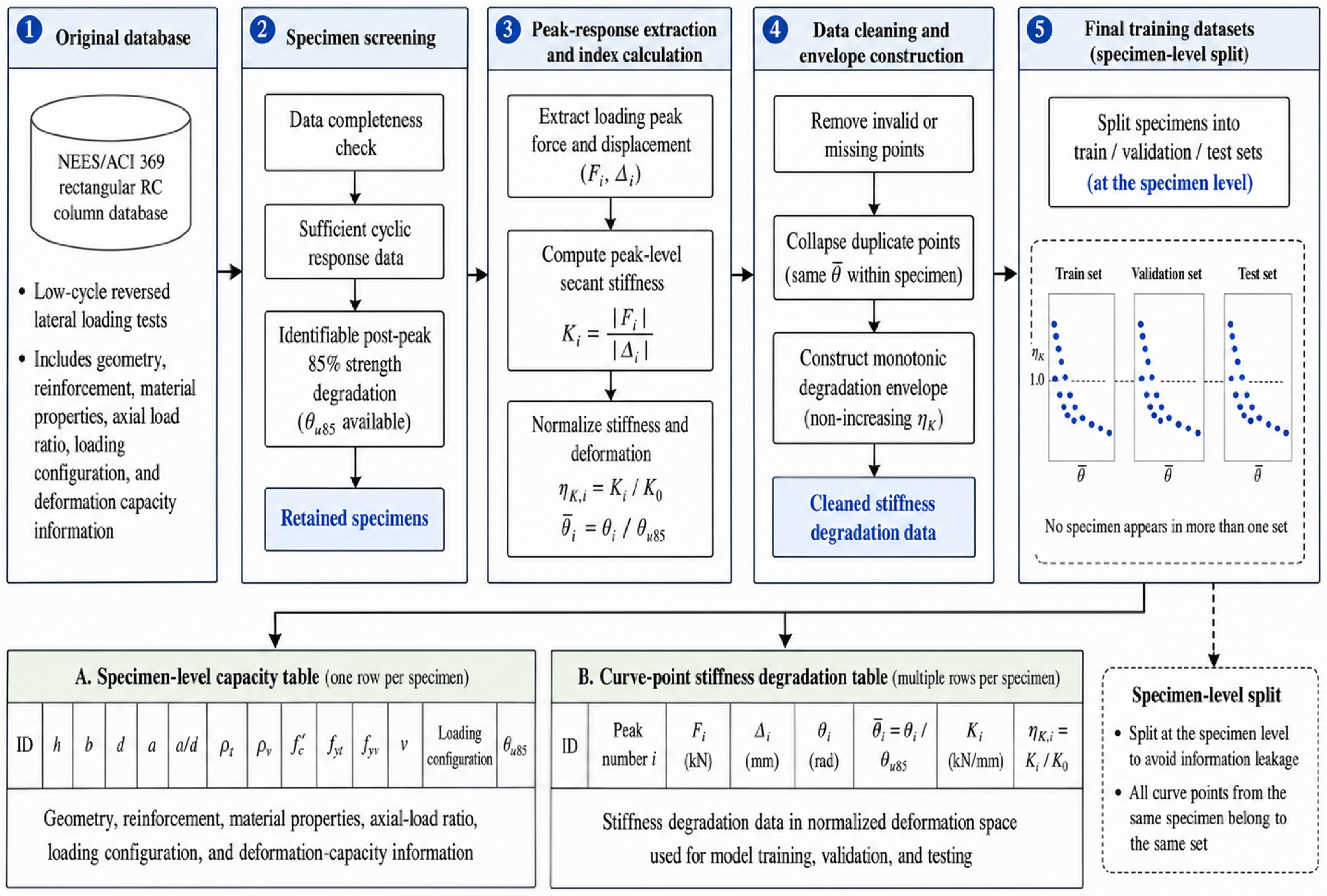
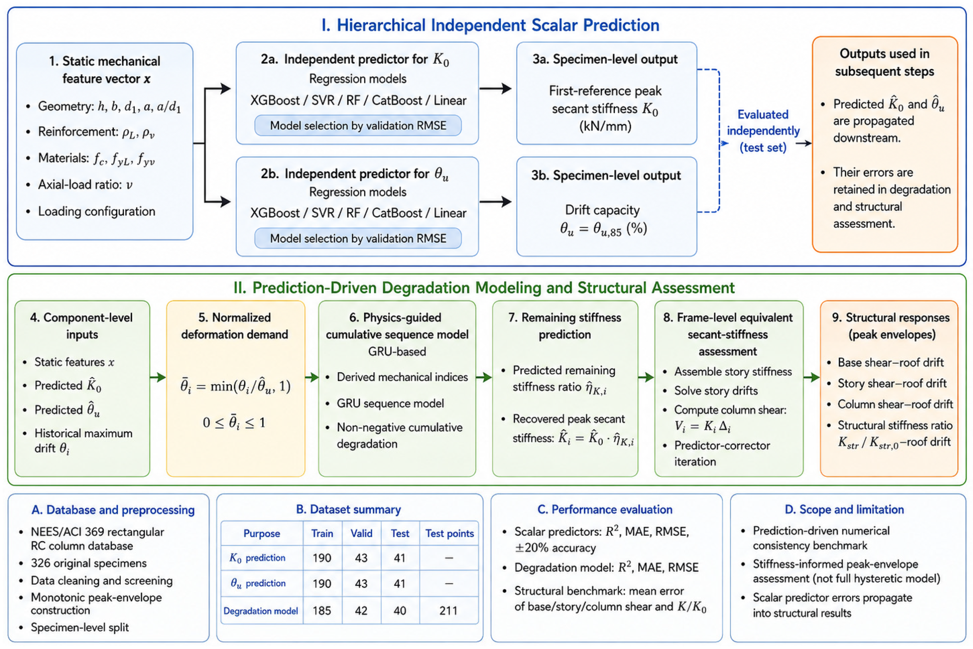
Figure 1 outlines the data-construction process. After screening, the records were organized into two complementary datasets. The capacity table contains one row per specimen and stores the static mechanical features, K₀, and θ_u. The curve-point table contains the peak-by-peak stiffness-degradation points extracted from each cyclic response and provides the sequences used for model training, validation, and testing.

Table 1. Variables and response quantities used in the hierarchical framework.

Category	Variable	Symbol	Description	Mechanical Relevance
Section geometry	Section depth	h	Column section dimension along the loading direction	Affects flexural stiffness and moment capacity
Section geometry	Section width	b	Column section dimension perpendicular to the loading direction	Affects section area and confinement region
Section geometry	Effective depth	d1	Effective depth of longitudinal reinforcement	Controls flexural lever arm
Member geometry	Shear–span length	a	Distance from the critical section to the lateral loading point	Controls bending–shear demand
Member geometry	Shear–span ratio	a/d1	Shear–span ratio based on effective depth	Distinguishes flexure- and shear-dominated behavior
Longitudinal reinforcement	Longitudinal reinforcement ratio	ρL	Ratio of longitudinal steel area to gross section area	Influences flexural strength and yielding
Transverse reinforcement	Transverse reinforcement ratio	ρv	Volumetric transverse reinforcement ratio	Influences confinement and cyclic degradation
Material property	Concrete compressive strength	fc	Concrete compressive strength	Affects cracking, compression damage, and stiffness
Material property	Longitudinal steel yield strength	fyL	Yield strength of longitudinal reinforcement	Affects flexural yielding
Material property	Transverse steel yield strength	fyv	Yield strength of transverse reinforcement	Affects confinement effectiveness
Axial loading	Axial-load ratio	ν	Normalized axial-load ratio	Influences stiffness, ductility, and degradation rate
Loading condition	Loading configuration	—	Single cantilever, double cantilever, or double curvature	Affects deformation mode and stiffness degradation path
Deformation capacity	85% post-peak drift capacity	θu	Drift ratio at 85% post-peak lateral strength (θu ≡ θu85)	Separate scalar target; predicted value used to normalize deformation demand in the degradation and frame assessments

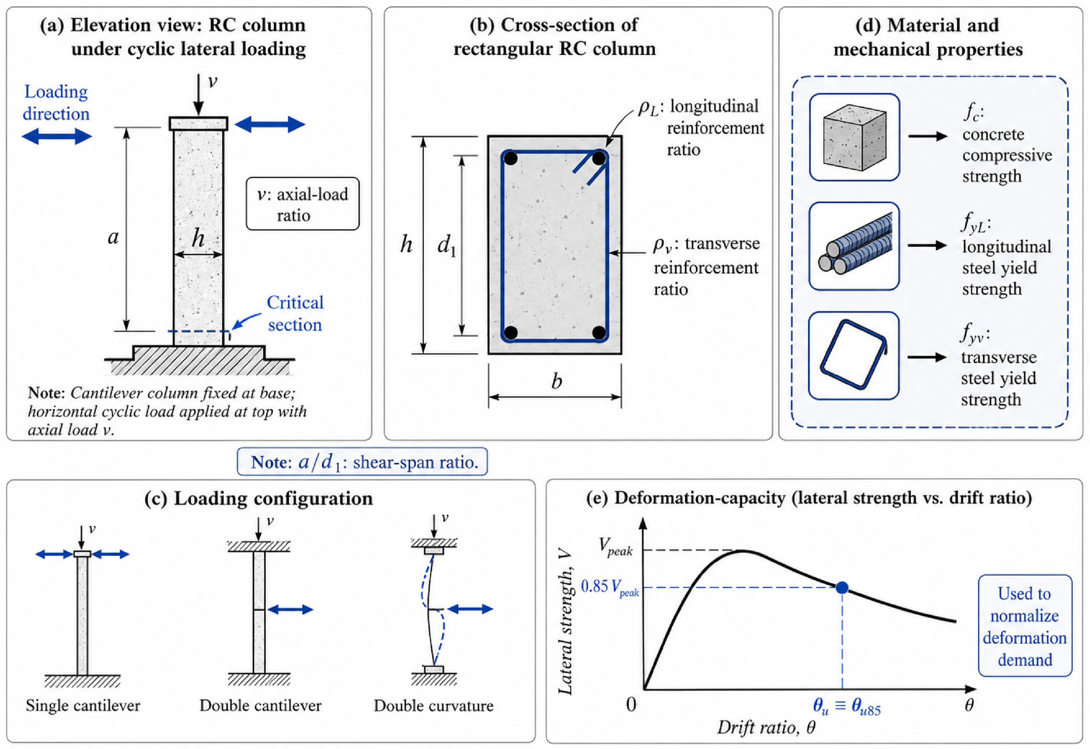
lists the variables and response quantities used in the framework, and Figure 2 defines the corresponding geometric, reinforcement, material, loading, and deformation-capacity parameters. These quantities are associated with cracking, yielding, confinement, shear–flexure interaction, axial-load effects, and cyclic deterioration in RC columns.

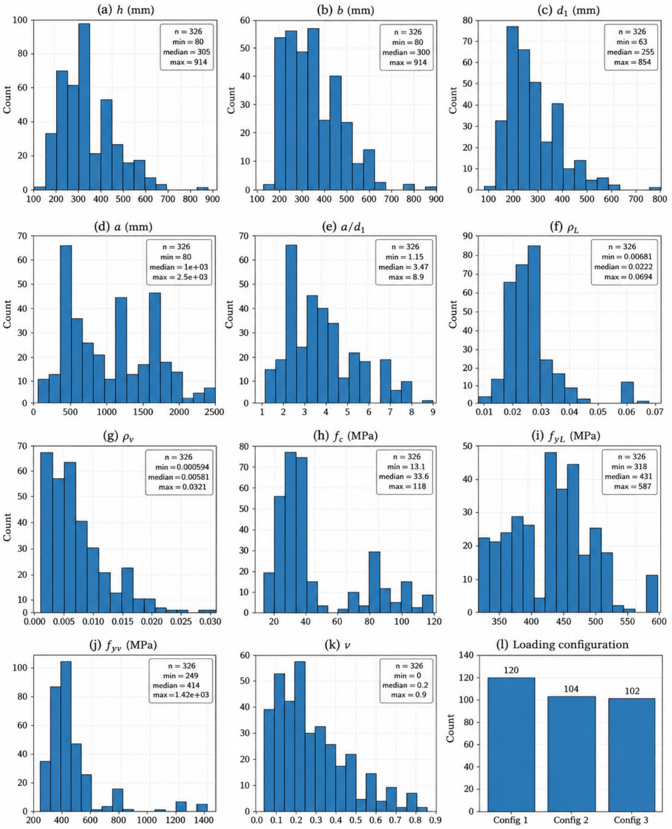
Figure 3 summarizes the distributions and ranges of the candidate variables in the original 326-specimen database. Section dimensions h and b range from approximately 80 to 914 mm, effective depth d₁ from 63 to 854 mm, shear–span length from 80 to 2500 mm, and shear–span ratio a/d₁ from 1.15 to 8.90. The longitudinal and transverse reinforcement ratios range from 0.0068 to 0.0694 and from 0.00059 to 0.0321, respectively. Concrete compressive strength ranges from 13.1 to 118 MPa. The longitudinal and transverse reinforcement yield strengths range from 318 to 587 MPa and from 249 to 1424 MPa, respectively, and the axial-load ratio ranges from 0 to 0.90. The three loading configurations contain 120, 104, and 102 specimens. Although the database spans broad parameter ranges, several variables are clustered or right-skewed. Only records that satisfied the completeness and response-quality criteria were retained for model development.

The broad parameter ranges in Figure 3 primarily reflect the inherent heterogeneity of the public database. After quality screening, this broad coverage was intentionally retained rather than narrowed to a more homogeneous subset, because it allows the model to be evaluated across diverse column configurations and tests whether specimen-specific descriptors can distinguish degradation paths that a single global function cannot represent. Range coverage alone, however, does not imply uniform information content. Several variables are clustered or sparsely represented near the tails, and coverage of each variable considered separately does not guarantee dense coverage of the full multivariate parameter space. The conclusions are therefore restricted to interpolation within the retained ranges, and predictions for sparsely represented or unseen parameter combinations should be interpreted cautiously.

2.2. Stiffness Degradation Index

For each retained loading peak, the cyclic secant stiffness is defined as

$$K_i={\displaystyle \frac{\left|F_i\right|}{\left|{\Delta }_i\right|}}$$

(1)

The force and displacement are taken at the same positive or negative loading peak. Absolute values place both loading directions on a common positive stiffness scale, while each peak remains a separate data point.

The normalized stiffness coefficient is defined as

$${\eta }_{K,i}={\displaystyle \frac{K_i}{K_0}}$$

(2)

Here, K₀ is the secant stiffness at the first valid reference peak after data cleaning. The coefficient η_K,i therefore denotes the fraction of K₀ retained at the i-th loading peak. K₀ is a reference peak secant stiffness and should not be interpreted as the uncracked elastic tangent stiffness.

The absolute peak deformation coordinate is

$${\theta }_i=\left|{\theta }_{i,peak}\right|$$

(3)

The deformation coordinate supplied to the machine-learning (ML) model is normalized as

$${\overline{\theta }}_i=\min \left({\displaystyle \frac{{\theta }_i}{{\widehat{\theta }}_u}},1.0\right)$$

(4)

The capacity θ_u is the drift ratio at which the post-peak lateral-strength envelope falls to 85% of its maximum value in the source database (θ_u ≡ θ_u85). It provides a common deformation-capacity scale without changing the peak secant stiffness defined in Equation (1). The measured θ_u is the target of the scalar predictor, whereas the independently predicted θ_u is used to normalize deformation demand in the degradation-model evaluation and the frame-level benchmark.

Concrete compressive strength is included because it is reported consistently across the database; concrete peak strain, ultimate strain, tension-softening parameters, reinforcement yield strain, ultimate strain, and bar-buckling strain are not available in a sufficiently complete and harmonized form. Their effects are only represented indirectly through measured K₀, θ_u, reinforcement ratios, strengths, confinement-related indices, and the observed peak envelopes. The model therefore predicts an empirical member-level stiffness path rather than a material stress–strain law, and omission of explicit strain variables is a limitation, particularly for post-yield and near-failure response.

2.3. Data Preprocessing and Quality Control

The preprocessing steps are summarized in Figure 1. Peak-response points were removed when force, displacement, drift ratio, stiffness, or deformation-capacity information was missing or invalid. For each remaining peak, the secant stiffness, normalized stiffness coefficient, and normalized deformation coordinate were calculated as described in Section 2.2.

A monotonic degradation envelope was then constructed for each specimen. Because the target describes stiffness loss with increasing historical maximum deformation, η_K was required to be non-increasing along the normalized deformation coordinate. This treatment suppresses local fluctuations caused by measurement noise, directional asymmetry, repeated cycles, or unstable post-peak response. The target is thus a cleaned peak-response envelope rather than the raw cyclic record.

Positive and negative peaks are retained as separate observations before envelope construction, but the sign is removed by the absolute secant-stiffness definition and the historical-maximum deformation coordinate. Repeated points at the same or nearly the same demand are collapsed. Therefore, the present target intentionally does not preserve push–pull asymmetry or cycle-count-dependent deterioration at approximately constant amplitude. Explicit treatment of these effects would require signed peak sequences, paired directional observations, and additional history variables such as cycle count or cumulative dissipated energy, together with sufficiently complete data for consistent model training.

Data were partitioned by specimen rather than by individual curve point. All points from a given specimen were assigned to the same training, validation, or test set, which limits information leakage and tests performance on unseen specimens. The capacity dataset contains 190 training, 43 validation, and 41 test specimens. After duplicate points were collapsed, the degradation dataset contains 185 training specimens (1016 points), 42 validation specimens (213 points), and 40 test specimens (211 points). The original specimen-level assignment was retained for the K₀, θ_u, and degradation tasks; specimens without eligible degradation points do not appear in the curve-point dataset. The reduction from 326 original records to 274 scalar-model specimens and 267 degradation-model specimens reflects the availability of valid scalar targets and cleaned degradation sequences after quality control.

3. Hierarchical Prediction Framework

3.1. Overall Framework

Figure 4 summarizes the complete workflow from static mechanical descriptors to independent scalar predictions, normalized deformation demand, degradation-path prediction, and frame-level equivalent secant-stiffness assessment. The static feature vector x is supplied to separate specimen-level models for K₀ and θ_u. Their outputs, K₀ and θ_u, are propagated to the subsequent calculations. The degradation submodel combines the static features with an ordered deformation sequence normalized by θ_u, and the predicted remaining stiffness ratio is multiplied by K₀ when absolute peak secant stiffness is required.

$${\widehat{K}}_0=f_K\left(x\right),\hspace{1em}{\widehat{\theta }}_u=f_{\theta }\left(x\right);\hspace{1em}{\overline{\theta }}_i=\min \left({\displaystyle \frac{{\theta }_i}{{\widehat{\theta }}_u}},1.0\right),\hspace{1em}{\widehat{\eta }}_{K,i}=f_{\eta }\left(x,{\overline{\theta }}_{1:i}\right),\hspace{1em}{K}_i={\widehat{K}}_0{\widehat{\eta }}_{K,i}$$

(5)

The scalar models are evaluated separately before their predictions are passed to the degradation and structural calculations. This arrangement keeps the accuracy of each task visible while allowing errors in $\hat{\mathrm{K}}$₀ and $\hat{\mathsf{\theta }}$_u to carry through to the downstream benchmarks.

The component-to-frame transition rests on four physical idealizations. First, the learned state is the peak secant-stiffness envelope governed by historical maximum drift. Second, the remaining stiffness of each column can be represented by a scalar secant quantity at a prescribed peak state. Third, story stiffness is assembled from the current column stiffnesses under floor-displacement compatibility. Fourth, peak column shear follows V = KΔ at that state. These hypotheses preserve a direct connection between the learned target and the structural calculation, but they exclude path-dependent unloading, independent strength deterioration, local hinge spread, and joint deformation.

3.2. Independent Prediction Model for K₀ and θ_u

Separate specimen-level regression models were trained for the first-reference peak secant stiffness K₀ and the drift capacity θ_u ≡ θ_u85 using the static mechanical feature vector x. Both targets are positive and right-skewed across specimens with different geometry, reinforcement, material properties, axial-load levels, and loading configurations. Logarithmic transformations were therefore applied:

$${\widehat{y}}_K=f_K\left(x\right),\hspace{1em}{y}_K=\ln \left(K_0\right),\hspace{1em}{\widehat{K}}_0=\exp \left({\widehat{y}}_K\right)$$

(6)

$${\widehat{y}}_{\theta }=f_{\theta }\left(x\right),\hspace{1em}{y}_{\theta }=\ln \left({\theta }_u\right),\hspace{1em}{\widehat{\theta }}_u=\exp \left({\widehat{y}}_{\theta }\right)$$

(7)

The inverse exponential transformation guarantees positive predictions. As defined in Section 2.2, K₀ is the first-reference peak secant stiffness, not the uncracked elastic tangent stiffness. The capacity θ_u is the drift ratio at which the post-peak strength envelope decreases to 85% of its maximum value.

Five tabular regression methods were considered for each target: linear regression, support vector regression (SVR), random forest, XGBoost, and CatBoost. The two tasks used the same candidate algorithms, input features, preprocessing steps, and specimen-level partitions, but were trained and optimized independently. Their errors are reported separately before their predictions are used in the degradation and structural calculations.

For the scalar tasks, linear regression provides an interpretable low-capacity baseline, SVR represents a kernel-based nonlinear alternative, random forest captures nonlinear interactions through bagged trees, and XGBoost and CatBoost provide gradient-boosted tree ensembles. The same candidate set was evaluated independently for K₀ and θ_u because the two targets have different distributions and governing sensitivities. Model selection was based on validation RMSE after training-only preprocessing, and the untouched test partition was used once for final reporting. This separation avoids choosing an algorithm from favorable test-set behavior.

3.3. Modeling Task and Input–Output Representation

The degradation submodel predicts the peak secant stiffness path extracted from cyclic column tests as historical maximum deformation increases. Each point corresponds to one retained loading peak, with K_i = |F_i|/|Δ_i| as defined in Section 2.2. The output is a monotonic peak-response envelope rather than a full hysteresis loop.

For each specimen, the model maps the static feature vector and the ordered normalized deformation sequence to a sequence of stiffness coefficients. Here, an “ordered normalized deformation sequence” refers to the retained peak-response points arranged in non-decreasing order of historical maximum drift and normalized by the independently predicted drift capacity ${\widehat{\theta }}_u$, ${\overline{\theta }}_i=\min \left({\displaystyle \frac{{\theta }_i}{{\widehat{\theta }}_u}},1.0\right)$. This sequence is a machine-learning data representation rather than a FEMA- or ACI-prescribed loading protocol. Because protocol-step labels are not used as model inputs, peak-response points obtained from different laboratory loading protocols can be represented within the same normalized deformation space after preprocessing.

$$\left\{x,{\overline{\theta }}_1,{\overline{\theta }}_2,\dots ,{\overline{\theta }}_n\right\}\to \left\{{\eta }_{K,1},{\eta }_{K,2},\dots ,{\eta }_{K,n}\right\}$$

(8)

In Equation (8), x denotes the static column feature vector, and η_K,i the corresponding normalized peak secant stiffness. The index i refers to a peak-response point, not to a complete loading cycle. The task is therefore formulated as sequence-to-sequence prediction in normalized deformation space.

The absolute peak secant stiffness is recovered, when required, from

$$K_i={\widehat{K}}_0{\widehat{\eta }}_{K,i}$$

(9)

where K₀ is the independently predicted first-reference peak secant stiffness. Thus, the recovered K_i includes uncertainty from K₀, while the normalized deformation coordinate includes uncertainty from θ_u. Both sources of error are carried into the downstream absolute-stiffness and structural-response calculations.

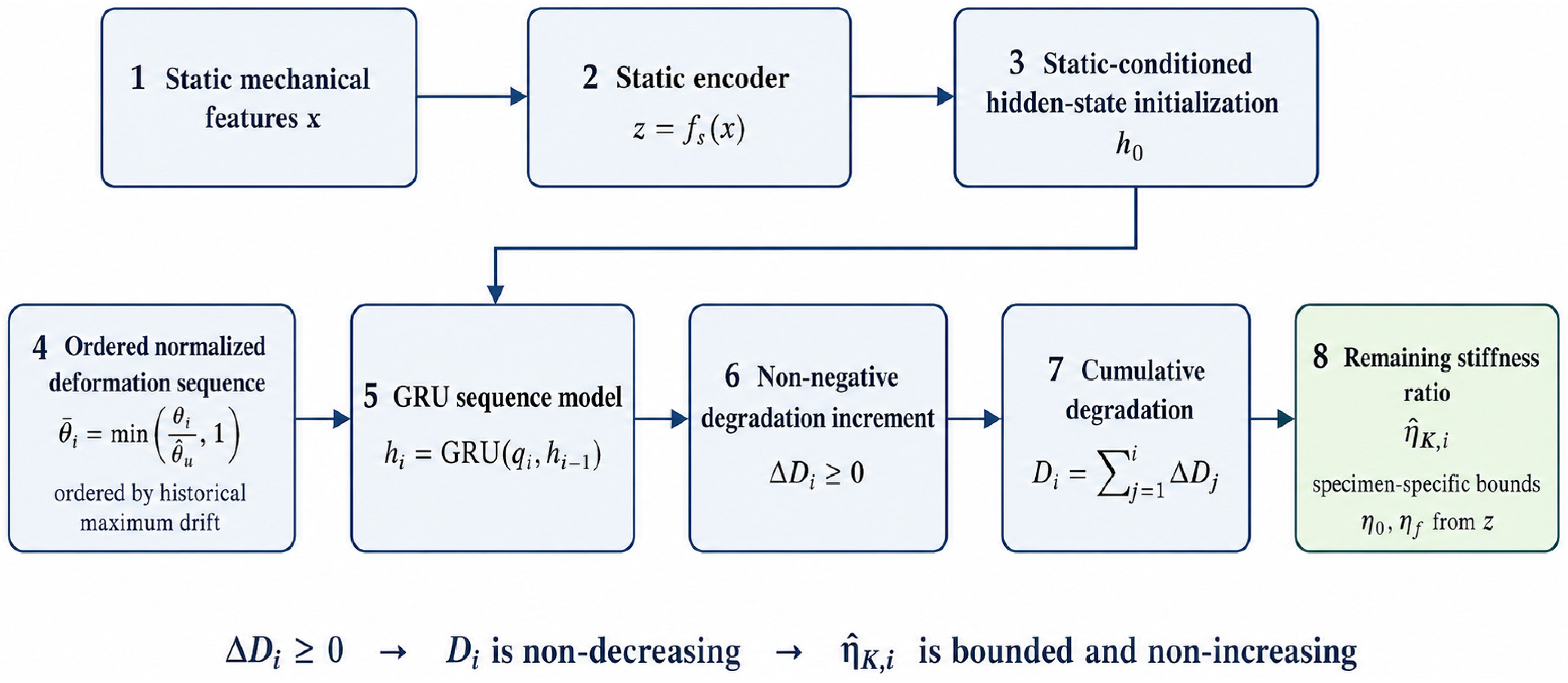
Figure 5 shows the architecture of the degradation submodel.

3.4. Physics-Guided Input Features

The model combines static specimen descriptors with deformation-dependent inputs. Static variables include section dimensions h and b, effective depth d₁, shear–span length a, shear–span ratio a/d₁, longitudinal and transverse reinforcement ratios, concrete and steel strengths, axial-load ratio ν, and loading configuration.

Derived mechanical indices augment these variables by representing relative confinement, longitudinal reinforcement contribution, and interactions with axial load.

$${\xi }_c={\displaystyle \frac{{\rho }_v{f}_{yv}}{f_c}}$$

(10)

The longitudinal reinforcement-strength index is defined as

$${\xi }_l={\displaystyle \frac{{\rho }_L{f}_{yL}}{f_c}}$$

(11)

The indices ξc and ξl represent the relative contributions of transverse confinement and longitudinal reinforcement, respectively. Axial–confinement and axial–shear–span indices are introduced to describe interactions between axial load and member properties:

$${\chi }_c={\displaystyle \frac{\nu }{{\xi }_c+\epsilon }}$$

(12)

$${\chi }_s={\displaystyle \frac{\nu }{a/d_1}}$$

(13)

A small positive constant ε is added to avoid numerical instability when ξc is close to zero.

At the i-th degradation point, the dynamic input vector combines normalized deformation with selected mechanical interactions:

$$q_i=\left({\overline{\theta }}_i,\Delta {\overline{\theta }}_i,{\overline{\theta }}_i\nu ,{\overline{\theta }}_i\left(a/d_1\right),{\displaystyle \frac{{\overline{\theta }}_i}{{\xi }_c+\epsilon }}\right)$$

(14)

where

$$\Delta {\overline{\theta }}_i=\max \left({\overline{\theta }}_i-{\overline{\theta }}_{i-1},0\right)$$

(15)

is the positive increment in normalized deformation. Its inclusion reflects the irreversible envelope formulation: degradation depends on accumulated historical maximum deformation rather than on instantaneous drift alone.

3.5. Cumulative Sequence Model with Monotonic Degradation Constraint

The architecture contains a static feature encoder, a GRU sequence branch, and a head that predicts non-negative degradation increments. The static feature vector is first mapped to a latent representation:

$$z_s=E_s\left(x\right)$$

(16)

where $E_s\left(\cdot \right)$ denotes the static encoder. The encoded vector ${\mathbf{z}}_s$ is used to initialize or condition the hidden state of the GRU sequence model:

$$h_0=W_h{z}_s+b_h$$

(17)

At each normalized deformation point, the GRU updates the hidden state according to the dynamic input vector ${\mathbf{q}}_i$:

$$h_i=\mathrm{GRU}\left(q_i,h_{i-1}\right)$$

(18)

The hidden state is converted to a non-negative degradation increment through a softplus activation:

$$\Delta D_i=\mathrm{softplus}\left[g_{\varphi } \left(h_i\right)\right]\Delta {\overline{\theta }}_i$$

(19)

The degradation-increment head maps the hidden state to an incremental deterioration variable. Because the softplus output is non-negative and is multiplied by a positive deformation increment, the predicted degradation increment satisfies

$$\Delta D_i\ge 0$$

(20)

The cumulative degradation variable is

$$D_i={\displaystyle \sum _{k=1}^i\Delta }{D}_k$$

(21)

The normalized stiffness coefficient is then obtained through a bounded exponential transformation:

$${\widehat{\eta }}_{K,i}={\eta }_f+\left({\eta }_0-{\eta }_f\right)\exp \left(-D_i\right)$$

(22)

The upper and lower stiffness levels, η₀ and ηf, depend on the specimen. In the final implementation, η₀ = 0.70 + 0.30σ(q₀(z)) and η_f = 0.25σ(qf(z)), where z is the encoded static feature vector and σ is the sigmoid function. Non-negative increments make D_i non-decreasing, so ηK,i remains bounded and non-increasing without post-processing.

3.6. Conventional Degradation Baselines

Four fixed-form functions were fitted as conventional baselines. Each expresses the normalized stiffness coefficient as a single global function of normalized deformation and does not use specimen-specific mechanical features.

The constant baseline is

$${\eta }_K\left(\overline{\theta }\right)=c_0$$

(23)

where c₀ is the mean retained stiffness ratio fitted to the training data.

The linear baseline is

$${\eta }_K\left(\overline{\theta }\right)=\max \left(c_0-c_1\overline{\theta },{\eta }_{\min }\right)$$

(24)

where c₀ and c₁ are fitted parameters and η_min prevents negative stiffness ratios.

The exponential baseline is

$${\eta }_K\left(\overline{\theta }\right)=c_0\exp \left(-c_1\overline{\theta }\right)$$

(25)

where c₀ controls the initial retained stiffness and c₁ the degradation rate.

The power-law baseline is

$${\eta }_K\left(\overline{\theta }\right)=c_0{\left(1+\overline{\theta }\right)}^{-c_1}$$

(26)

where c₀ and c₁ are fitted parameters.

Baseline parameters were obtained by minimizing the mean squared error over the cleaned training points. The fitted parameters were then held fixed for evaluation on the independent test specimens. All baselines and the sequence model used the same specimen-level split and were compared using R², MAE, and RMSE.

3.7. Training Strategy, Loss Function, and Evaluation Metrics

The K₀, θ_u, and degradation models were trained with the same fixed specimen-level partitions. Validation performance was used to select the scalar models, while the degradation submodel was trained on the cleaned peak-by-peak sequences. Predicted ${\widehat{\theta }}_u$ values from the selected scalar model defined the normalized deformation coordinates used by the degradation submodel. An out-of-fold cascade was not implemented for normalization of the training partition. Because the scalar predictor used to generate training-partition ${\widehat{\theta }}_u$ values was fitted using those specimens, this choice can introduce optimistic bias into degradation-model training. This limitation concerns the training-partition cascade; the reported test degradation metrics are still evaluated on unseen test specimens using predicted ${\widehat{\theta }}_u$. A fully out-of-fold cascade is therefore identified as a priority for future robustness assessment.

Static and dynamic inputs were standardized using statistics from the training set only. Because the valid sequence length differs among specimens, padded entries were removed from the loss through sequence masking.

The degradation submodel was optimized using a weighted Smooth L1 loss between predicted and measured normalized stiffness coefficients:

$$\mathcal{L}={\displaystyle \frac{{\displaystyle \sum _{s=1}^N{\displaystyle \sum _{i=1}^{n_s}{m}_{s,i}}}{w}_{s,i}\mathrm{SmoothL}1\left({\widehat{\eta }}_{K,s,i}-{\eta }_{K,s,i}\right)}{{\displaystyle \sum _{s=1}^N{\displaystyle \sum _{i=1}^{n_s}{m}_{s,i}}}{w}_{s,i}}}$$

(27)

where $N$ is the number of training specimens, $n_s$ is the number of valid degradation points for specimen $s$, $m_{s,i}$ is the sequence mask, and $w_{s,i}$ is the point weight. A larger weight was assigned to the final valid point of each degradation curve because the late-stage response controls the terminal stiffness deterioration trend.

The main hyperparameters were a 64-dimensional static latent space, a GRU hidden dimension of 96, two GRU layers, dropout of 0.10, and a batch size of 16. Training used AdamW with a learning rate of 1.0 × 10⁻³, weight decay of 1.0 × 10⁻⁴, and a Smooth L1 transition parameter of 0.05. A maximum of 900 epochs and an early-stopping patience of 140 epochs were specified; the checkpoint with the lowest validation RMSE was retained.

The Smooth L1 transition parameter β = 0.05 was selected on the normalized stiffness-ratio scale, for which a residual magnitude of 0.05 corresponds to five percentage points of K₀. Under the Smooth L1 formulation, residual magnitudes below β lie in the quadratic region, whereas larger residuals lie in the linear region. Thus, β = 0.05 provides quadratic sensitivity to deviations smaller than five percentage points of normalized stiffness while limiting the leverage of larger residuals. It was fixed before final test evaluation; the independent test set was not used to tune β.

A smaller β would make the loss nearly absolute-error-like for most observations and could reduce sensitivity to meaningful small deviations; a much larger β would keep more large residuals in the quadratic region and allow atypical irregular curves to dominate optimization. The adopted value is therefore a scale-based robustness choice rather than a universal material constant. A formal β-sensitivity or nested hyperparameter study remains appropriate future work.

Performance was assessed using the coefficient of determination (R²), mean absolute error (MAE), and root-mean-square error (RMSE):

$$R^2=1-{\displaystyle \frac{{\displaystyle \sum _i{\left({\eta }_{K,i}^{\mathrm{true}}-{\widehat{\eta }}_{K,i}\right)}^2}}{{\displaystyle \sum _i{\left({\eta }_{K,i}^{\mathrm{true}}-{\overline{\eta }}_K^{\mathrm{true}}\right)}^2}}}$$

(28)

$$\mathrm{MAE}={\displaystyle \frac{1}{n}}{\displaystyle \sum _{i=1}^n\left|{\eta }_{K,i}^{\mathrm{true}}-{\widehat{\eta }}_{K,i}\right|}$$

(29)

$$\mathrm{RMSE}=\sqrt{{\displaystyle \frac{1}{n}}{\displaystyle \sum _i{\left({\eta }_{K,i}^{\mathrm{true}}-{\widehat{\eta }}_{K,i}\right)}^2}}$$

(30)

The same metrics were used for the sequence model and the four global degradation functions.

K₀ and θ_u were evaluated at specimen level. Degradation performance was evaluated with pooled peak-level metrics under normalization by predicted drift capacity, so these metrics include uncertainty in $\hat{\mathsf{\theta }}$_u. Uncertainty in $\hat{\mathrm{K}}$₀ does not affect normalized η_K and enters only when absolute stiffness and structural responses are recovered.

4. Component-Level Prediction Results

4.1. Prediction Performance of K₀ and θ_u

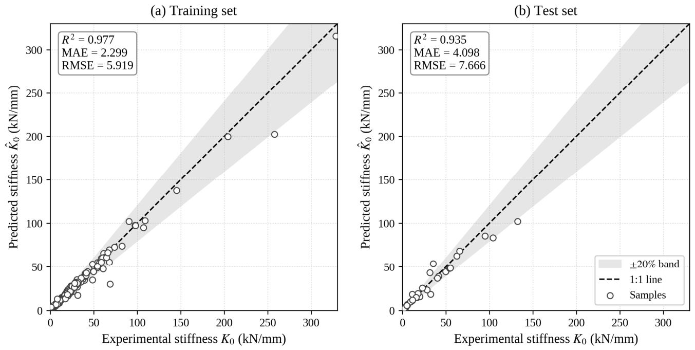
Five regression algorithms were assessed for K₀ and θ_u. Model selection used validation-set RMSE, and the independent test set was reserved for the final evaluation. Figure 6 and Figure 7 compare measured and predicted values for the training and test sets.

The selected XGBoost model achieved R² = 0.977, MAE = 2.299 kN/mm, and RMSE = 5.919 kN/mm on the training set (Figure 6). On the test set, R² was 0.935, MAE was 4.098 kN/mm, and RMSE was 7.666 kN/mm. The ±20% bounds contained 91.4% of the training predictions and 82.5% of the test predictions. Most test points cluster near the 1:1 line in the densely sampled low- and intermediate-stiffness range; the larger deviations occur at high K₀, where few specimens are available.

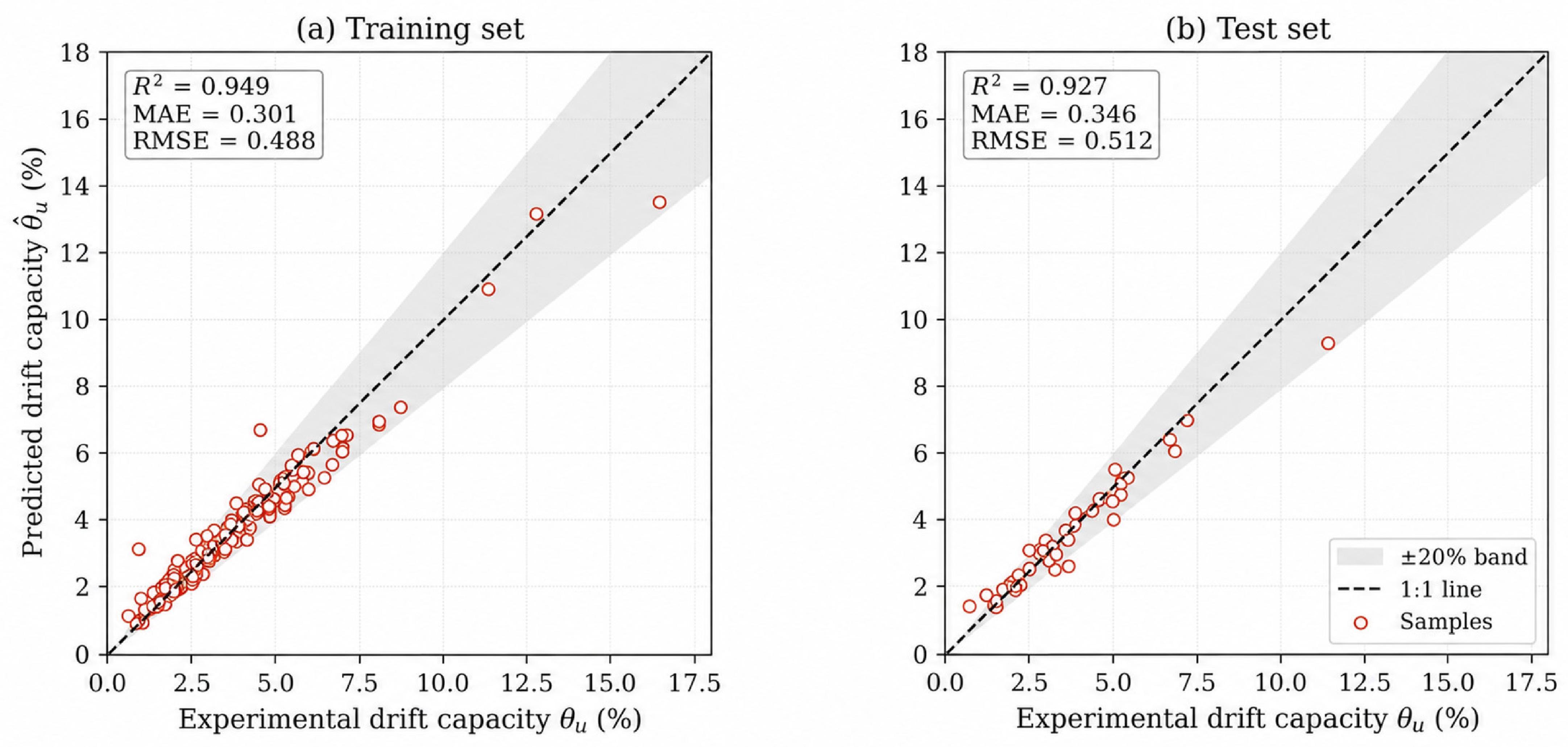
For θ_u, the selected CatBoost model achieved R² = 0.949, MAE = 0.301 percentage points, and RMSE = 0.488 percentage points on the training set (Figure 7). The test-set values were R² = 0.927, MAE = 0.346 percentage points, and RMSE = 0.512 percentage points. Predictions within the ±20% bounds accounted for 92.4% of the training set and 87.5% of the test set. Training and test errors are similar over the main data range, while the sparsely sampled high-capacity region shows larger deviations.

These results show that the available geometric, reinforcement, material, axial-load, and loading-configuration variables contain sufficient information to estimate K₀ and θ_u within the retained database. The two predictors are reported separately here before their outputs are passed to the degradation and frame-level calculations.

4.2. Degradation Prediction Under Predicted Deformation-Capacity Normalization

The degradation submodel was evaluated using specimen-level training, validation, and independent test sets, with deformation normalized by the independently predicted $\hat{\mathsf{\theta }}$_u. Its reported error therefore combines uncertainty from the drift-capacity predictor and the degradation model. After duplicate-point collapse and monotonic-envelope construction, the test set contains 211 points from 40 RC column specimens.

Table 2. Test-set results: Global degradation functions versus the proposed sequence model.

Model	R2	MAE	RMSE
Constant	−0.0025	0.2563	0.2924
Linear	0.3934	0.1802	0.2275
Exponential	0.4185	0.171	0.2227
Power-law	0.4132	0.1727	0.2237
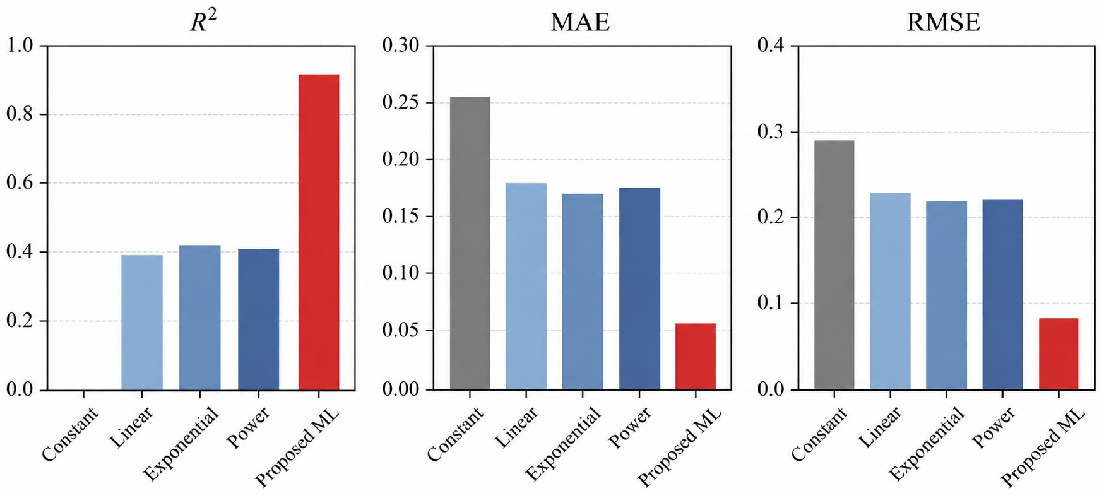
Proposed sequence model	0.9272	0.0542	0.0788

and Figure 8 report the test results. The model achieved R² = 0.9272, MAE = 0.0542, and RMSE = 0.0788 for normalized peak stiffness. Compared with the best global function, RMSE decreased from 0.2227 to 0.0788, and R² increased from 0.4185 to 0.9272. Because the target is a stiffness ratio, these metrics include uncertainty in $\hat{\mathsf{\theta }}$_u but not in $\hat{\mathrm{K}}$₀.

4.3. Comparison with Conventional Degradation Baselines

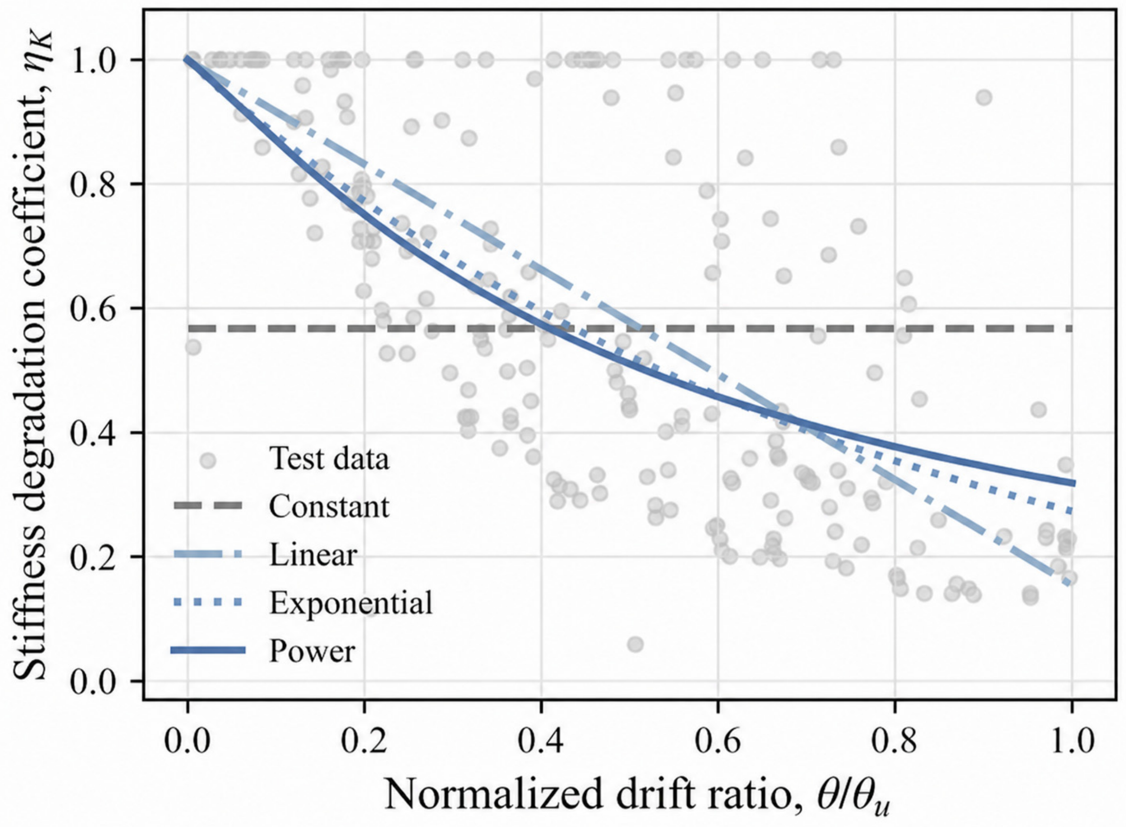
The sequence model produced substantially smaller test errors than the four fixed-form baselines. The exponential function was the strongest conventional model, with R² = 0.4185 and RMSE = 0.2227; the linear and power-law functions performed similarly, and the constant function could not represent deformation-dependent stiffness loss.

A single global curve can follow only the average degradation trend. It cannot account for the distinct paths associated with differences in geometry, reinforcement, material strength, axial load, shear–span ratio, loading configuration, and deformation capacity.

Figure 9 makes this limitation clear. The fixed-form curves follow the overall trend but not the specimen-to-specimen scatter, especially at intermediate and large normalized demands. The sequence model is better able to represent these differences within the sampled parameter range. This comparison tests the value of specimen-dependent modeling against global functions; it does not isolate the contribution of the GRU architecture or the monotonic constraint.

4.4. Error Distribution for Different Column Groups

To examine performance across the test set, errors were grouped by loading configuration, axial-load ratio, shear–span ratio, and transverse reinforcement ratio (

Table 3. (a) Grouped test-set errors by loading configuration and axial-load ratio. (b) Grouped test-set errors by shear–span ratio and transverse reinforcement ratio.

(a)
Group	Category	Number of Points	Number of Specimens	R2	MAE	RMSE
Loading configuration	Double cantilever	25	11	0.9405	0.0425	0.0835
Loading configuration	Double curvature	62	13	0.8927	0.0616	0.0932
Loading configuration	Single cantilever	124	16	0.9355	0.0529	0.0694
Axial-load ratio	ν ≤ 0.10	22	6	0.8434	0.0701	0.0882
Axial-load ratio	0.10 < ν ≤ 0.30	132	19	0.9342	0.0511	0.0734
Axial-load ratio	ν > 0.30	57	15	0.9139	0.0554	0.0867
(b)
Group	Category	Number of Points	Number of Specimens	R2	MAE	RMSE
Shear–span ratio	a/d1 ≤ 2.0	10	4	0.786	0.0476	0.0667
Shear–span ratio	2.0 < a/d1 ≤ 4.0	111	18	0.9327	0.0497	0.0755
Shear–span ratio	a/d1 > 4.0	90	18	0.9155	0.0606	0.0839
Transverse reinforcement ratio	ρᵥ ≤ 0.004	49	11	0.9286	0.0495	0.0658
Transverse reinforcement ratio	0.004 < ρᵥ ≤ 0.008	87	14	0.903	0.0623	0.0915
Transverse reinforcement ratio	ρᵥ > 0.008	75	15	0.9458	0.0479	0.0703

a,b).

For the three loading configurations, R² was 0.9405 for double-cantilever specimens, 0.8927 for double-curvature specimens, and 0.9355 for single-cantilever specimens. The slightly larger error for double-curvature tests may reflect their different moment distribution and deformation compatibility.

The low-, medium-, and high-axial-load groups yielded R² values of 0.8434, 0.9342, and 0.9139, respectively. The lower value for the low-axial-load group is based on only six specimens; MAE and RMSE are more comparable across the medium- and high-ratio groups.

For a/d₁ ≤ 2.0, 2.0 < a/d₁ ≤ 4.0, and a/d₁ > 4.0, the corresponding R² values were 0.7860, 0.9327, and 0.9155. The short-column subgroup contains only 10 points from four specimens and may also be more strongly affected by shear–flexure interaction, so its result is descriptive rather than conclusive.

For low, medium, and high transverse reinforcement ratios, R² was 0.9286, 0.9030, and 0.9458, respectively. Because some groups contain few specimens, these values should be read together with MAE, RMSE, and subgroup size.

4.5. Representative Curve-Level Predictions

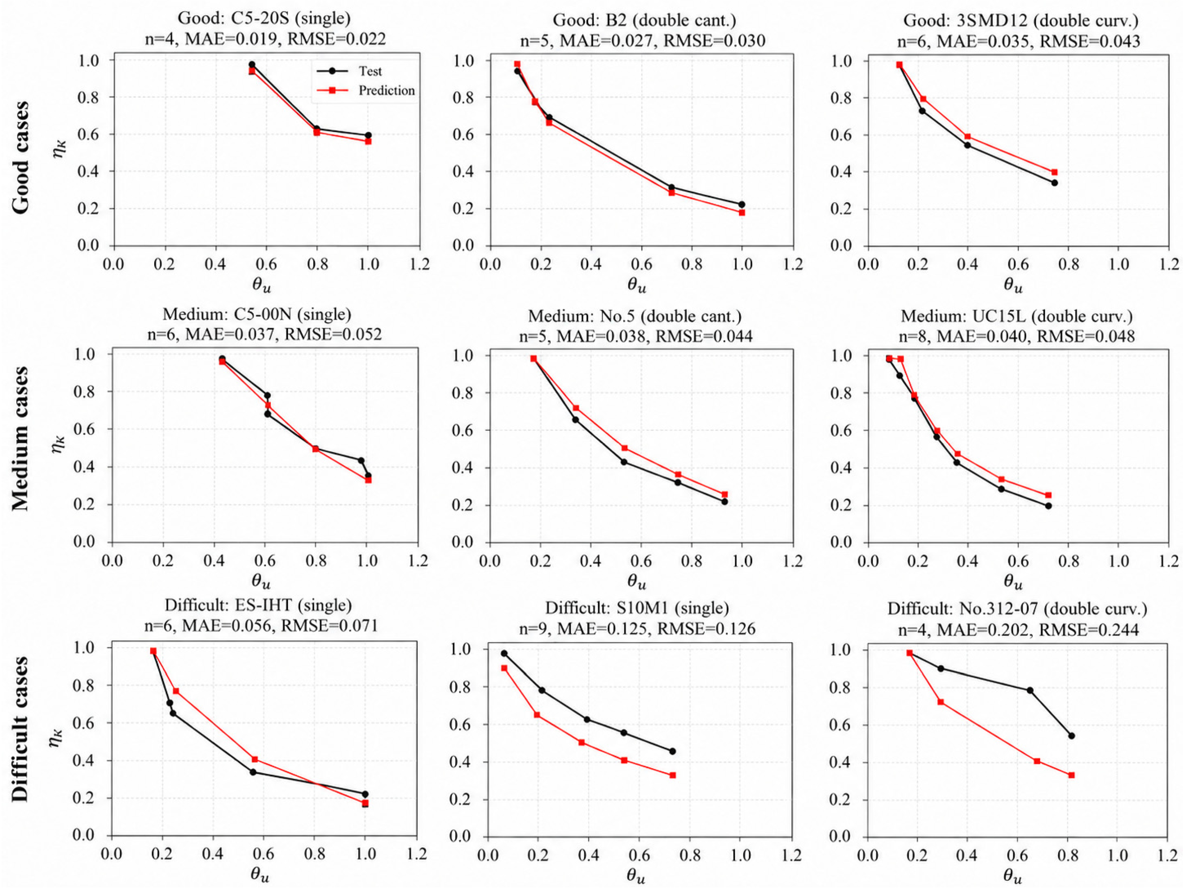
Curve-level predictions were examined to assess how well the model reproduces the shape of the stiffness-degradation path. Figure 10 includes good, intermediate, and difficult cases spanning different path shapes and, where possible, different loading configurations. The examples were selected to show the range of observed behavior rather than only a best–median–worst ordering.

In the good and intermediate cases, the predictions follow the measured paths, including the rapid early stiffness loss and the slower decline at larger normalized demands. This shape is typical of the cleaned peak-response envelopes in the database.

The difficult cases remain monotonic but either underpredict or overpredict stiffness over part of the deformation range. Their errors may be related to irregular degradation, short shear spans, post-peak instability, or changes in the governing mechanism. Failure-mode descriptors or mechanism-specific model branches may improve these cases.

The curve comparisons show that the model captures the dominant degradation shape for many unseen specimens, while also revealing cases that are not fully described by the current feature set.

5. Frame-Level Assessment Using Predicted Component Stiffness

5.1. Equivalent Secant-Stiffness Updating Formulation

At frame level, the predicted $\hat{\mathrm{K}}$₀, $\hat{\mathsf{\theta }}$_u, and stiffness-degradation ratio are used as component inputs to the structural calculation. For column i in story j, the effective stiffness and normalized historical drift at iteration m are updated as follows:

$$K_{c,ij}^{\mathrm{eff},(m)}={\widehat{K}}_{c0,ij}{\widehat{\eta }}_{K,ij}^{(m)},\hspace{1em}\hspace{1em}{r}_{ij}^{(m)}=\min \left({\displaystyle \frac{{\theta }_{\max ,ij}^{(m)}}{{\widehat{\theta }}_{u85,ij}}},1.0\right)$$

(31)

The component model supplies the remaining peak secant stiffness ratio at a specified historical maximum drift. It does not define a separate strength-degradation law or a complete unloading–reloading relation. Because $\hat{\mathrm{K}}$₀ and $\hat{\mathsf{\theta }}$_u are prescribed for each column, errors from both scalar models are retained in the updated stiffness and structural response.

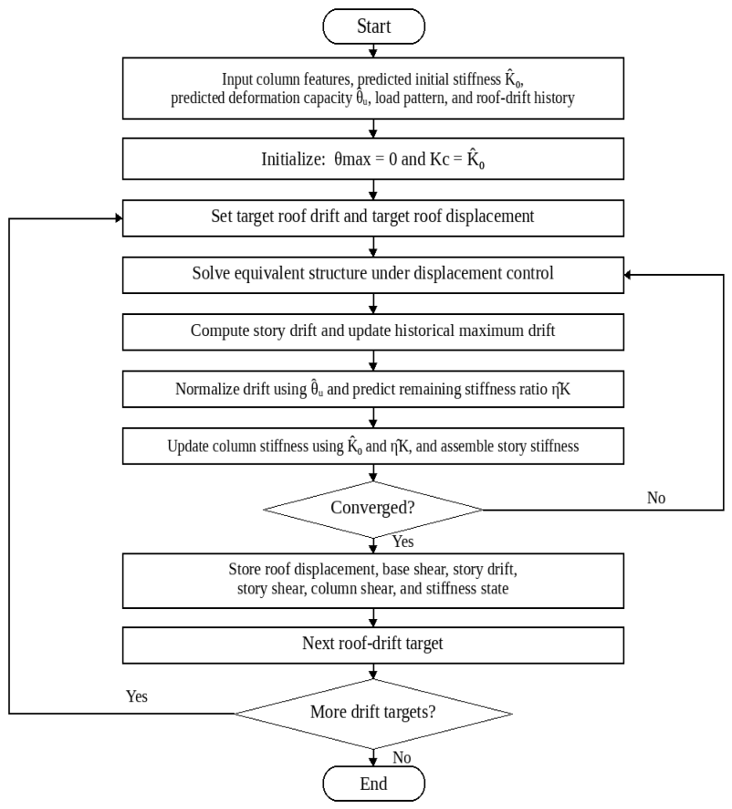
The frame is analyzed through iterative updates of equivalent secant stiffness. Predicted column stiffnesses are assembled into story stiffnesses, which control the displacement and drift distribution. At each imposed peak state, column shear is calculated directly as V = KΔ from the updated secant stiffness and interstory displacement. No separate force cap, strength envelope, or learned strength-loss rule is used.

As shown in Figure 11, an inner predictor–corrector loop updates stiffness at each prescribed roof-drift target, while an outer loop advances through the roof-drift amplitude sequence. The degradation state is governed by the historical maximum drift rather than the current signed drift.

The frame is idealized as an equivalent shear-type system. Equation (31) defines the column effective stiffness and normalized historical drift demand.

The equivalent lateral stiffness of story $j$ is then assembled from the effective stiffnesses of all columns in that story:

$$K_{s,j}^{(m)}={\displaystyle \sum _i{K}_{c,ij}^{\mathrm{eff},(m)}}$$

(32)

For a prescribed roof-drift target ${\theta }_{r,n}$, the corresponding target roof displacement is

$$u_{r,\mathrm{target}}={\theta }_{r,n}H$$

(33)

where $H$ is the total height of the frame. Under a predefined lateral load vector $\mathbf{p}$, the displacement-controlled equivalent system is solved as

$$K^{(m)}{u}^{(m)}={\lambda }^{(m)}p$$

(34)

The load factor is chosen so that the target roof displacement is satisfied:

$${\lambda }^{(m)}={\displaystyle \frac{u_{r,\mathrm{target}}}{e_r^T{\left(K^{(m)}\right)}^{-1}p}}$$

(35)

The corresponding displacement vector is

$$u^{(m)}={\lambda }^{(m)}{\left(K^{(m)}\right)}^{-1}p$$

(36)

where ${\mathbf{e}}_r$ is the selector vector for the roof displacement degree of freedom. The story drift demand obtained from the structural response is

$${\theta }_j^{(m)}={\displaystyle \frac{u_j^{(m)}-u_{j-1}^{(m)}}{h_j}}$$

(37)

Here, the floor displacements define the drift of story j, and h_j is the associated story height. Because stiffness degradation depends on the largest prior demand, the historical maximum drift is updated as

$${\theta }_{\max ,ij}^{(m)}=\max \left({\theta }_{\max ,ij}^{(m-1)},\left|{\theta }_j^{(m)}\right|\right)$$

(38)

The normalized demand passed to the degradation model is

$$r_{ij}^{(m)}=\min \left({\displaystyle \frac{{\theta }_{\max ,ij}^{(m)}}{{\widehat{\theta }}_{u85,ij}}},1.0\right)$$

(39)

where ${\widehat{\theta }}_{u85,ij}$ is the independently predicted drift ratio corresponding to 85% of the post-peak lateral strength of the corresponding component. The upper bound of 1.0 is imposed to avoid unsupported extrapolation beyond the deformation range represented by the component-level degradation database. The trained degradation model then predicts the remaining stiffness ratio as

$${\widehat{\eta }}_{K,ij}^{(m)}=f_{\mathrm{ML}}\left(x_{ij},r_{ij}^{(m)}\right)$$

(40)

Story drift is converted to interstory displacement by

$${\Delta }_j^{(m)}={\theta }_j^{(m)}{h}_j$$

(41)

Column shear at the current peak state is then obtained from the updated secant stiffness:

$$V_{c,ij}^{(m)}=K_{c,ij}^{\mathrm{eff},(m)}{\Delta }_j^{(m)}$$

(42)

At each imposed roof-drift target, a predictor–corrector iteration is used because the drift distribution depends on the current stiffness state, while the stiffness state depends on the updated drift demand. The structure is first solved using the stiffness state inherited from the previous target drift. The resulting story drifts are then used to update $r_{ij}$, ${\eta }_{K,ij}$, $K_{c,ij}^{\mathrm{e}\mathrm{f}\mathrm{f}}$, and $K_{s,j}$. The equivalent structure is reanalyzed under the same roof-displacement target until the change in story stiffness becomes sufficiently small:

$${\max }_j\left|{\displaystyle \frac{K_{s,j}^{(m+1)}-K_{s,j}^{(m)}}{K_{s,j}^{(m)}}}\right|<{\epsilon }_K$$

(43)

After convergence at a roof-drift target, the procedure stores roof displacement, base shear, story drift, story shear, column shear, story stiffness ratio, and column ηK. Story shear is the sum of the column shears in that story, and base shear equals the first-story shear. The calculation then proceeds to the next target amplitude.

5.2. Illustrative Application to a Representative Frame

A representative three-story frame is used to illustrate the updating procedure. The example demonstrates its implementation; it is not intended as a design prototype or an independent validation case. The broader numerical benchmark is presented in Section 6.

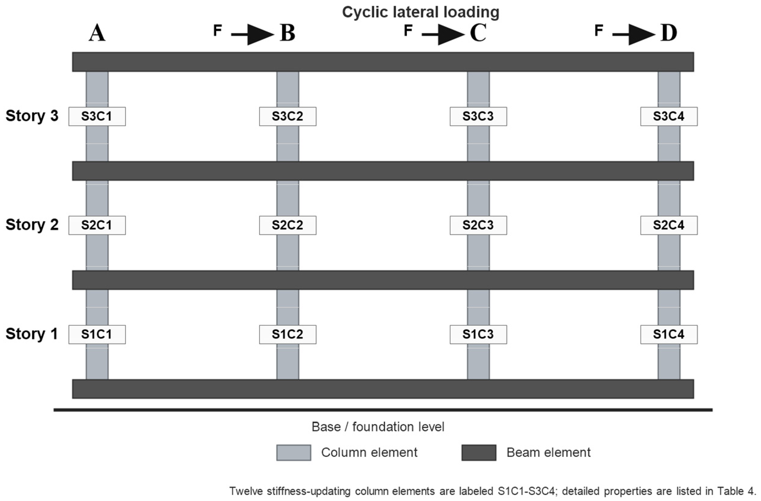
The frame is represented as a three-story shear system with a story height of 3300 mm and four RC columns per story. All four column lines within a story use the same experimental specimen properties, so story stiffness is assembled from four identical updated column stiffnesses. In the three-story four-bay planar frame, A, B, C and D denote the four column axes, and F represents the cyclic lateral force applied at the top-floor level.

Table 4. Column properties and predicted inputs for the illustrative three-story frame.

Story	Specimen	Loading	h × b (mm)	a/d1	ρL (%)	ρv (%)	fc (MPa)	ν	$\hat{\mathsf{\theta }}$u (%)	$\hat{\mathbf{K}}$0 (kN/mm)
1	NC	Double cantilever	457.0 × 457.0	3.49	1.94	0.52	39.8	0.310	2.28	35.98
2	D16	Double curvature	300.0 × 300.0	1.15	1.69	0.42	26.1	0.230	3.24	5.41
3	BG-7	Single cantilever	350.0 × 350.0	5.40	2.93	0.51	34.0	0.462	4.59	11.44

lists the column properties and predicted scalar inputs, and Figure 12 shows the adopted frame.

Beam degradation is not modeled separately. The beams transfer floor shear and enforce lateral-displacement compatibility among the column lines, while stiffness updates are applied only to the columns. This idealization isolates how column stiffness degradation affects story-level and global response.

The frame is subjected to prescribed cyclic roof-drift amplitudes. At each amplitude, the calculation updates the historical maximum story drift, predicts the remaining column stiffness, assembles the story stiffnesses, and derives column, story, and base shears. Stored quantities include roof displacement, base shear, story drift, story shear, column shear, story stiffness ratio, and column η_K. 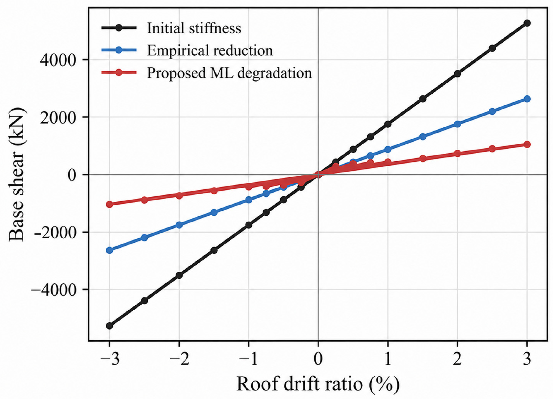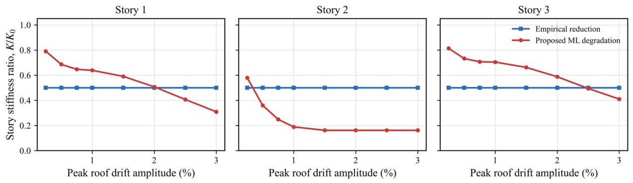Figure 13 and Figure 14 present the peak-response curves and story-stiffness ratios, respectively.

Figure 13 and Figure 14 illustrate why the three stiffness assumptions diverge. The initial-stiffness model retains K₀ and therefore produces the steepest force–displacement response. The constant 0.50K₀ reference imposes the same reduction at every amplitude and cannot reproduce either rapid early deterioration or the slower late-stage decline. The ML-updated response evolves with the predicted story-specific ${\widehat{\theta }}_u$ and member descriptors: the first-story NC columns have the largest ${\widehat{k}}_o$ but the smallest ${\widehat{\theta }}_u$, whereas the upper-story D16 and BG-7 columns have lower initial stiffness and larger predicted capacities. This contrast changes the drift distribution as degradation proceeds and explains why the story curves do not remain parallel. The discrepancy is therefore not evidence of three estimates of the same constitutive law; it is the expected consequence of comparing a demand-dependent component model with two deliberately simplified stiffness assumptions. Because the example lacks an experimental frame reference and omits beam/joint degradation, pinching, and P–Δ effects, Figure 13 and Figure 14 demonstrate transfer mechanics rather than validate force capacity.

Quantitatively, the illustrative stories also occupy distinct mechanical regimes: ${\widehat{k}}_o$ equals 35.98, 5.41, and 11.44 kN/mm from the first to third story, while ${\widehat{\theta }}_u$ equals 2.28%, 3.24%, and 4.59%, respectively. The first story begins much stiffer but reaches a larger fraction of its predicted capacity at a given story drift; the upper stories begin more flexible but retain a larger normalized deformation margin. The iterative solution therefore changes both the magnitude and vertical distribution of stiffness, which a uniform 0.50K₀ factor cannot reproduce.

6. Numerical Benchmark Against OpenSeesPy Fiber-Frame Models

6.1. Benchmark Objective and Logic

This section tests whether the component degradation model can be used for frame-level stiffness and peak-response assessment. Independent OpenSeesPy fiber-frame analyses serve as the nonlinear reference. The comparison therefore contrasts a fiber-section finite-element model with the equivalent secant-stiffness procedure introduced in Section 5.

The benchmark is a numerical consistency check, not experimental validation of complete RC frames. It examines: (1) peak base shear versus roof drift; (2) degradation of the structural secant-stiffness ratio; and (3) the distribution of story and column shear over the frame height. In the simplified model, shear is calculated as V = KΔ. Any plateau or reduction in peak shear therefore emerges from increasing deformation combined with declining secant stiffness, rather than from a prescribed strength-loss rule.

All benchmark calculations use predicted component inputs. The predicted $\hat{\mathrm{K}}$₀ and $\hat{\mathsf{\theta }}$_u are combined with the degradation ratio in the structural procedure, so the comparison includes errors from the scalar models, the degradation model, and their transfer to the frame analysis.

6.2. Fiber-Frame Reference Models and Lateral Load Pattern

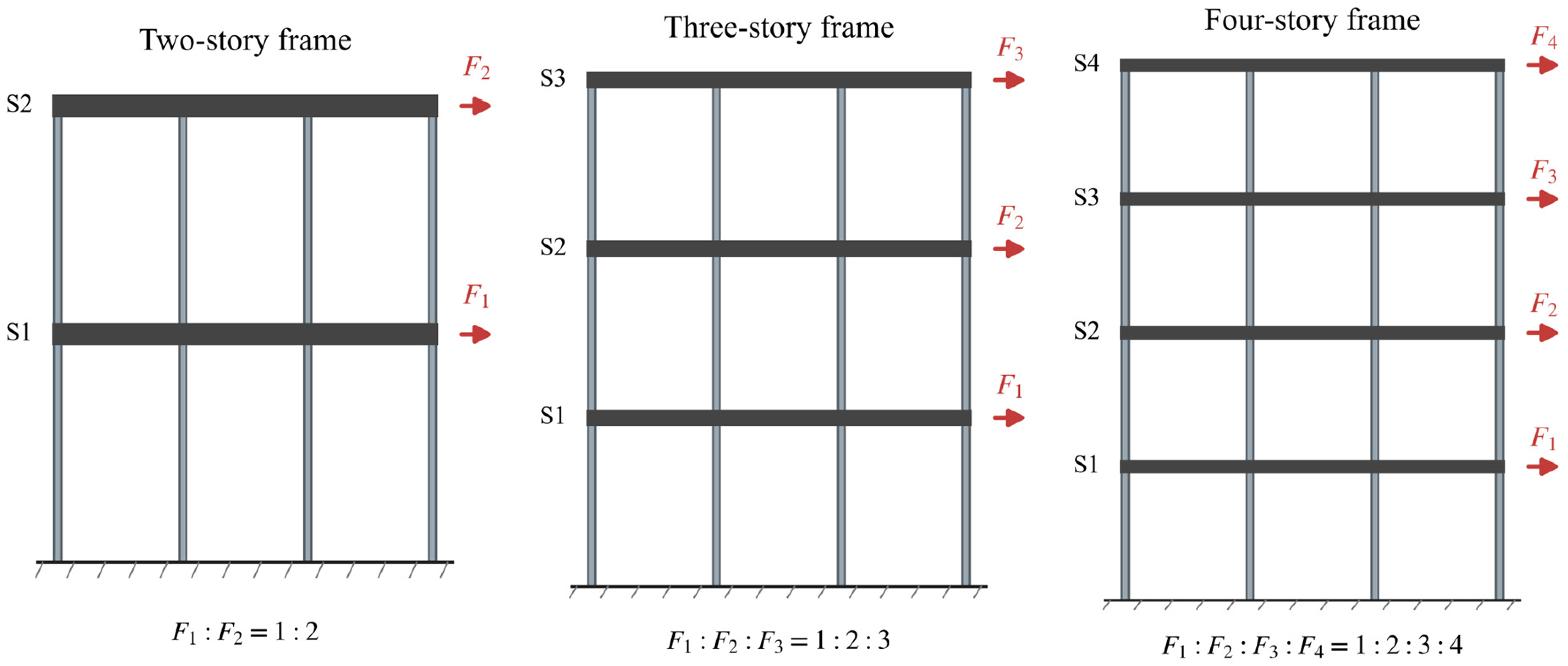
Twelve three-bay RC frames are considered: two-, three-, and four-story systems with four column lines and a story height of 3300 mm. Most frames have 5000 mm bays; one three-story case uses 6000 mm bays to introduce a modest geometric variation.

Table 5. Column parameters and predicted scalar inputs for the OpenSeesPy benchmark frames.

Case	Stories	Bay (mm)	h × b (mm)	a/d1	ρL (%)	ρv (%)	fc (MPa)	fy_l (MPa)	fy_t (MPa)	ν	$\hat{\mathsf{\theta }}$u (%)	$\hat{\mathbf{K}}$0 (kN/mm)
F2-U1	2	5000	305.0 × 305.0	1.72	2.44	0.15	29.9	461.9	413.9	0.104	2.61	6.19
F2-2SLH18	2	5000	457.2 × 457.2	3.71	1.94	0.07	33.1	330.9	399.9	0.070	2.98	32.87
F2-S4	2	5000	457.2 × 457.2	3.76	2.48	0.17	21.8	434.3	475.9	0.146	3.54	26.68
F2-U6	2	5000	350.0 × 350.0	3.28	3.31	0.85	37.3	436.9	424.9	0.131	4.35	11.98
F3-U1	3	5000	305.0 × 305.0	1.72	2.44	0.15	29.9	461.9	413.9	0.104	2.61	6.19
F3-U1-wide bay	3	6000	305.0 × 305.0	1.72	2.44	0.15	29.9	461.9	413.9	0.104	2.61	6.19
F3-S4	3	5000	457.2 × 457.2	3.76	2.48	0.17	21.8	434.3	475.9	0.146	3.54	26.68
F3-U6	3	5000	350.0 × 350.0	3.28	3.31	0.85	37.3	436.9	424.9	0.131	4.35	11.98
F3-2SLH18	3	5000	457.2 × 457.2	3.71	1.94	0.07	33.1	330.9	399.9	0.070	2.98	32.87
F4-U1	4	5000	305.0 × 305.0	1.72	2.44	0.15	29.9	461.9	413.9	0.104	2.61	6.19
F4-S4	4	5000	457.2 × 457.2	3.76	2.48	0.17	21.8	434.3	475.9	0.146	3.54	26.68
F4-U6	4	5000	350.0 × 350.0	3.28	3.31	0.85	37.3	436.9	424.9	0.131	4.35	11.98

lists the column parameters, and Figure 15 shows the frame layouts.

Beams are modeled as elastic transfer members, and columns as displacement-based beam-column elements with RC fiber sections. This matches the assumption in Section 5 that beam deterioration is not an independent state variable. The benchmark therefore isolates how column stiffness degradation is reflected in global, story-level, and column-level response.

Table 6. OpenSeesPy settings used in the fiber-frame reference analyses.

Item	Setting	Purpose or Note
Column element	dispBeamColumn	Displacement-based RC fiber-section beam-column element.
Concrete material	Concrete02	Separate confined-core and unconfined-cover materials; core compressive strength taken as 1.20fc.
Steel material	Steel02	Longitudinal reinforcement with fy from the database, Es = 200,000 MPa, b = 0.01.
Fiber discretization	Core 12 × 12; cover patches 4 × 12 and 12 × 3; 8 longitudinal bars	Used for every column section.
Integration scheme	Lobatto, 5 points	Used for each column beam-column element.
Beam model	elasticBeamColumn	Elastic transfer members; beam degradation is not modeled.
Floor compatibility	equalDOF in horizontal translation	All column-line nodes at the same floor share lateral displacement.
Geometric transformation	Linear	P–Δ effects are not explicitly included in the present reference set.
Axial load	Constant after gravity step	Applied from the prescribed axial-load ratio and then held constant.
Lateral loading	Roof DisplacementControl	Inverted triangular load pattern proportional to story level.
Convergence test	NormDispIncr, tolerance 1 × 10−6, max 120 iterations	Newton algorithm with ModifiedNewton fallback.
Response extraction	Base reactions and local element forces	Base shear from fixed-node reactions; column shear from localForce Vi.

lists the main OpenSeesPy settings. Fiber sections use separate confined-core and unconfined-cover concrete materials, and longitudinal reinforcement is represented by Steel02 with a strain-hardening ratio of 0.01. The axial load associated with each prescribed axial-load ratio is applied first and then held constant. Lateral forces follow an inverted triangular pattern proportional to story elevation: F₁:F₂ = 1:2 for two stories, F₁:F₂:F₃ = 1:2:3 for three stories, and F₁:F₂:F₃:F₄ = 1:2:3:4 for four stories. The equivalent shear-building model uses the same load pattern.

The member axial forces are applied from the prescribed database axial-load ratios during the gravity step and are then held constant during cyclic roof-displacement loading; no drift-dependent axial-load reduction factor is used. This isolates stiffness-transfer effects and keeps the simplified and fiber-frame models consistent. It does not represent overturning-induced axial-force redistribution, vertical-ground-motion effects, or strength loss that would change axial capacity, so applications in which those effects are important require a coupled frame model.

For interpretation and reproducibility, Table 6 should be read as a summary of the principal comparison settings rather than as a complete executable OpenSeesPy input specification. Exact reproduction additionally requires the beam elastic section properties and the complete Concrete02 parameter set used in the analysis scripts. The present benchmark also adopts a simplified confinement treatment: the confined-core compressive strength is prescribed as 1.20f_c, and no specimen-specific confinement relation based on ρ_v and transverse-steel strength is introduced. Consequently, transverse reinforcement enters the ML component predictor explicitly through its mechanical descriptors, whereas its influence is not represented one-to-one through a specimen-specific confinement law in the fiber reference. This model-form asymmetry is a limitation of the numerical benchmark and further supports interpreting it as a stiffness-transfer consistency check rather than as experimental validation of a fully calibrated frame model.

6.3. Loading Protocol and Response Extraction

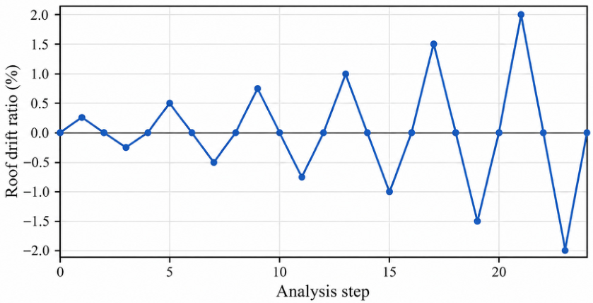
After the constant axial loads are applied, cyclic pushover analysis is performed under roof-displacement control. Roof-drift amplitudes of 0.25%, 0.50%, 0.75%, 1.00%, 1.50%, and 2.00% are imposed in both directions, with unloading to zero between excursions. The same sequence is used to extract peak responses from OpenSeesPy and to drive the simplified procedure. Figure 16 shows the loading protocol.

The imposed drift amplitudes are analysis checkpoints and are not assigned directly to Immediate Occupancy, Life Safety, or Collapse Prevention states. Such labels depend on component type, detailing, failure mode, axial load, and the acceptance criteria adopted by a particular standard. The source database does not provide a uniform code-based performance-state classification across all specimens, and retrospective assignment of IO/LS/CP labels would require specimen-specific detailing, failure-mode, and acceptance-criteria information that is not consistently available. The independently predicted ${\widehat{\theta }}_u$ provides the study-specific deformation-capacity scale, whereas code performance limits should be evaluated separately for the intended assessment context.

At each peak amplitude, base shear is obtained from the algebraic sum of horizontal reactions at the fixed base nodes. Story shear is calculated by summing column shears in a consistent global direction; absolute values are used only when reporting the envelope. Individual column shear is taken from the local force vector of each fiber column element. This extraction provides comparison quantities at global, story, and component levels.

6.4. Comparison Indices

The models are compared using mean relative errors in base shear, story shear, and column shear, together with the absolute error in structural secant-stiffness ratio. For a generic shear response V, the relative error at peak q is

$$e_V^{(q)}={\displaystyle \frac{\left|V_{\mathrm{ML}}^{(q)}-V_{\mathrm{FE}}^{(q)}\right|}{\max \left(\left|V_{\mathrm{FE}}^{(q)}\right|,\epsilon \right)}}\times 100\%$$

(44)

where the superscripts ML and FE denote the proposed ML-updated structural model and the OpenSeesPy fiber-frame reference, respectively, and $\epsilon$ is a small numerical tolerance introduced to avoid division by zero. Mean and maximum errors are then computed over all peak drift points and, where applicable, over all stories or columns.

The structural secant-stiffness ratio is calculated from peak base shear and roof displacement:

$${\eta }_{\mathrm{str}}^{(q)}={\displaystyle \frac{\left|V_b^{(q)}\right|/\left|u_r^{(q)}\right|}{K_{\mathrm{str},0}}}$$

(45)

where $V_b^{\left(q\right)}$ and $u_r^{\left(q\right)}$ are the base shear and roof displacement at the $q$-th peak drift point, respectively, and $K_{\mathrm{s}\mathrm{t}\mathrm{r},0}$ is the first nonzero peak secant stiffness of the corresponding model. The mean absolute stiffness-ratio error is calculated as

$$\Delta {\eta }_{\mathrm{str}}={\displaystyle \frac{1}{N_p}}{\displaystyle \sum _{q=1}^{N_p}\left|{\eta }_{\mathrm{str},\mathrm{ML}}^{(q)}-{\eta }_{\mathrm{str},\mathrm{FE}}^{(q)}\right|}$$

(46)

6.5. Benchmark Results Under Predicted Component Inputs

With predicted component inputs, the ML-updated procedure shows reasonable agreement with the OpenSeesPy reference. The reported errors combine contributions from $\hat{\mathrm{K}}$₀, $\hat{\mathsf{\theta }}$_u, the degradation path, and the simplified structural idealization.

Table 7. Error summary for the OpenSeesPy fiber-frame benchmark.

Case	Mean Base Shear Error (%)	Max Base Shear Error (%)	Mean Story Shear Error (%)	Mean Column Shear Error (%)	Mean |Δηstr|	Final ηstr (FE/ML)
F2-U1	21.88	34.32	18.39	19.11	0.055	0.270/0.206
F2-2SLH18	8.26	15.20	11.42	10.19	0.019	0.165/0.180
F2-S4	11.25	20.56	13.45	13.70	0.030	0.188/0.212
F2-U6	21.16	28.74	20.70	21.25	0.026	0.226/0.284
F3-U1	21.47	27.01	19.47	19.99	0.032	0.216/0.200
F3-U1-wide bay	21.53	26.93	19.52	19.94	0.031	0.216/0.200
F3-S4	11.88	20.35	16.56	16.64	0.040	0.157/0.200
F3-U6	18.41	29.41	19.44	19.72	0.044	0.183/0.266
F3-2SLH18	19.07	43.13	24.54	23.51	0.045	0.124/0.178
F4-U1	21.33	28.32	19.16	19.54	0.022	0.186/0.190
F4-S4	14.72	19.72	20.66	20.60	0.057	0.143/0.193
F4-U6	20.89	32.26	22.33	22.48	0.068	0.157/0.256

summarizes the aggregate results.

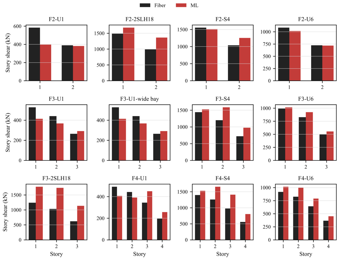
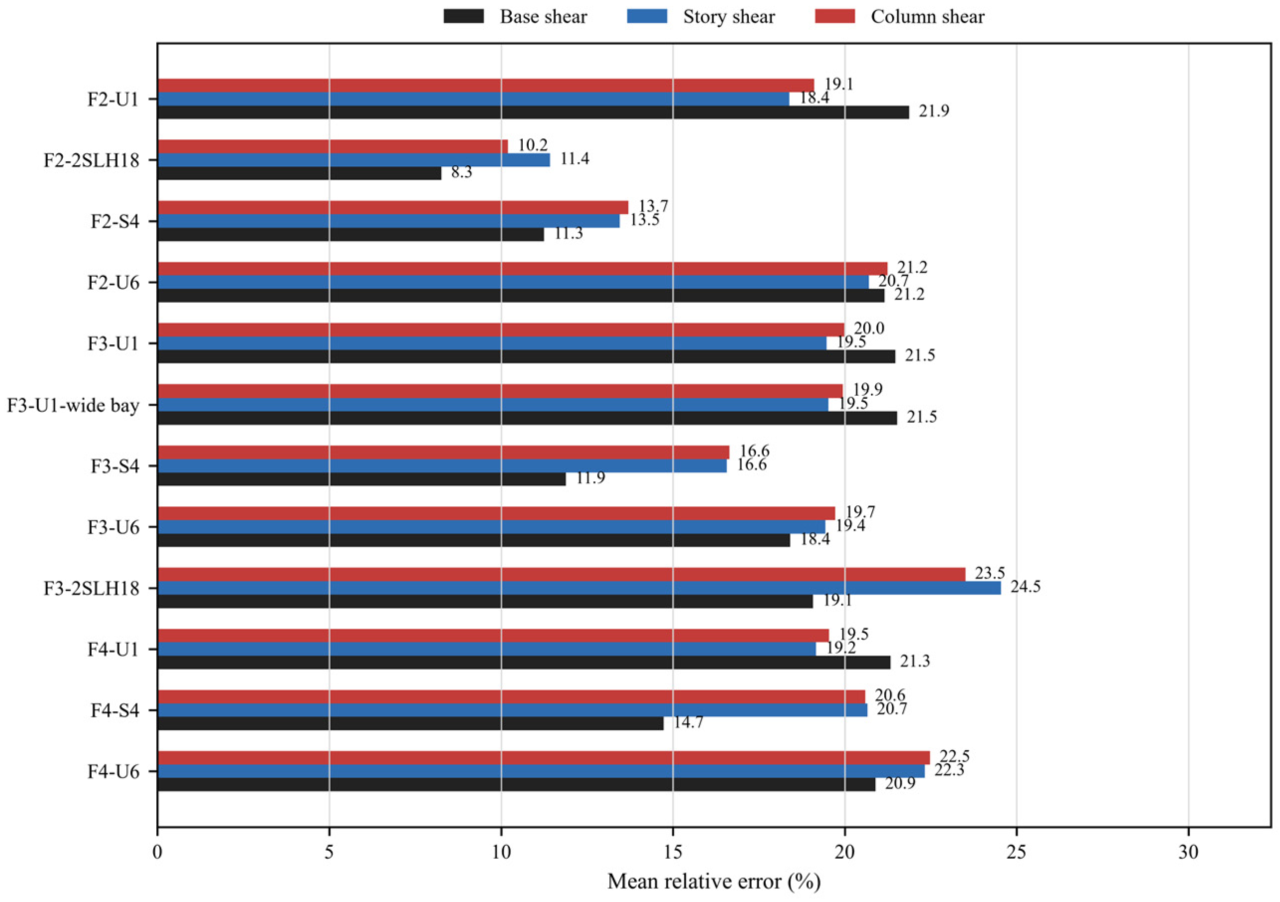
Figure 17 compares the mean errors in base shear, story shear, and column shear for the 12 cases. In most frames, the three measures are of similar magnitude, indicating that discrepancies are distributed across global, story, and component responses rather than concentrated at the base.

The error pattern is linked to both structural height and component selection. The two-story 2SLH18 case gives the lowest mean errors (8.26% in base shear and 10.19% in column shear) and the smallest mean stiffness-ratio error (0.019), whereas the three-story 2SLH18 and four-story U6 cases show larger story/column errors and stiffness-ratio discrepancies. Increasing story count adds redistribution opportunities that the shear-building idealization cannot reproduce after section yielding. The wide-bay U1 case is nearly indistinguishable from the corresponding standard-bay case because beams are elastic transfer members and member-level column inputs are unchanged; this confirms that the current formulation has limited sensitivity to bay-length effects.

No single design variable explains the benchmark error because component prediction error and structural idealization error interact. For example, the 5000-mm and 6000-mm U1 frames give almost identical errors, indicating that bay width has little effect under the adopted elastic-beam compatibility assumption. By contrast, increasing the U6 system from two to four stories raises the mean stiffness-ratio error from 0.026 to 0.068, consistent with accumulated redistribution that is not represented by independent story-level secant updates. These are benchmark-specific trends, not universal monotonic sensitivities.

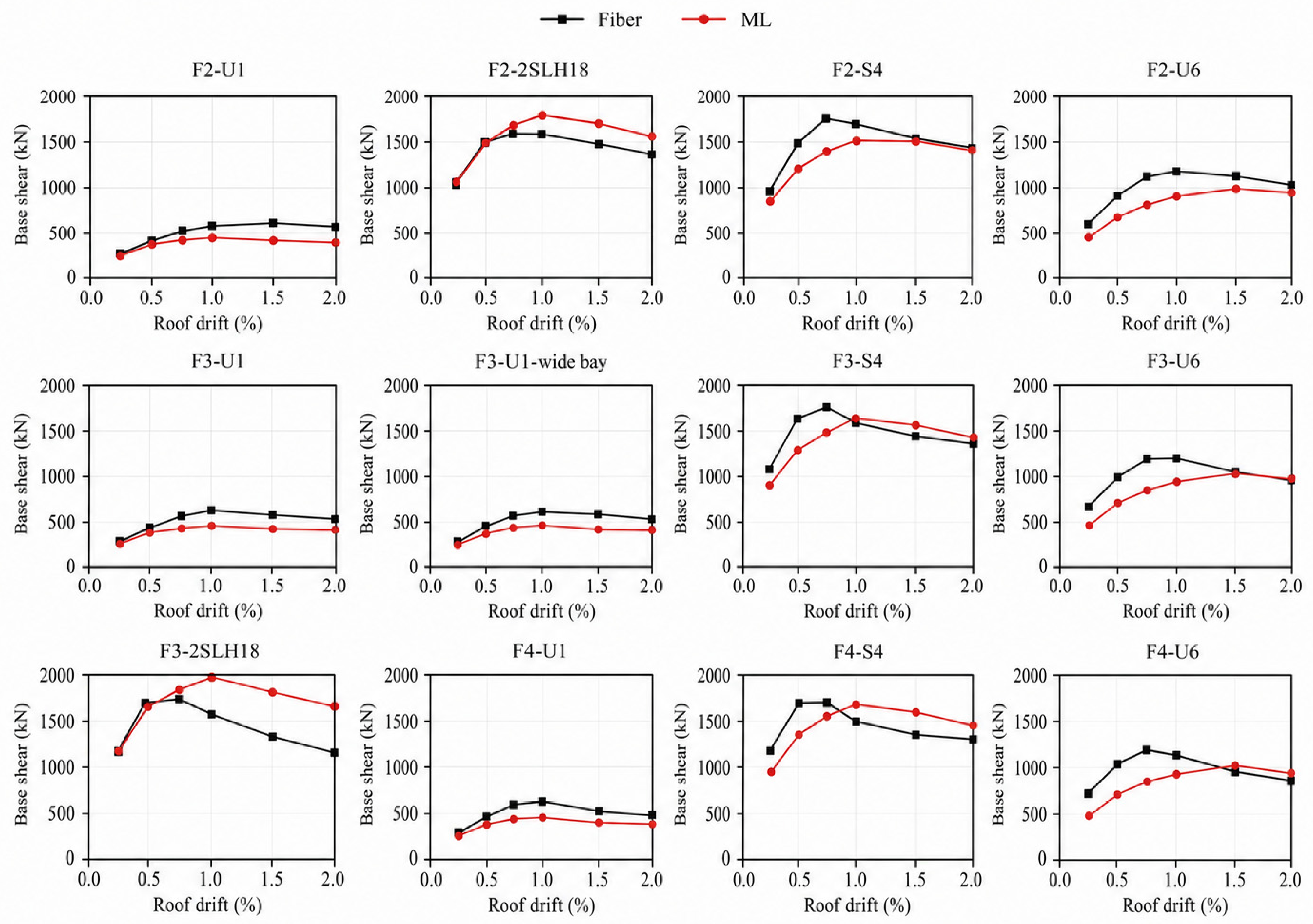
For several cases, the simplified procedure reproduces the main shape of the fiber-frame peak base-shear response, including a rising branch and, where present, a plateau or decline at larger drift. Because V = KΔ, this shape results from the balance between increasing displacement and decreasing secant stiffness; it is not an independently modeled strength-degradation response. Differences in peak force, peak drift, and post-peak slope remain because the fiber models resolve material nonlinearity, section yielding, and local redistribution. Figure 18 presents the base-shear comparisons.

The largest curve discrepancies occur where the fiber model develops material nonlinearity, section yielding, and redistribution that are absent from V = KΔ. For U1, the short shear–span ratio (a/d₁ = 1.72), low transverse reinforcement ratio, and small predicted ${\widehat{k}}_o$ and ${\widehat{\theta }}_u$ place the response near a regime in which shear–flexure interaction and local damage can strongly affect the force path. For U6, the higher longitudinal and transverse reinforcement and larger ${\widehat{\theta }}_u$ delay degradation in the learned component model. In the fiber benchmark, however, confinement is represented through the simplified fixed core-strength enhancement described in Section 6.2 rather than through a specimen-specific confinement law. The ML and fiber curves should therefore be compared primarily in terms of the transferred stiffness trend, not as two models with identical representation of transverse-reinforcement effects or exact peak-strength and post-peak behavior.

The magnitude of a force discrepancy must also be interpreted relative to the modeling target. The component model is optimized against η_K, whereas base, story, and column shears are derived outputs. A small bias in ${\widehat{k}}_o$ affects every force ordinate, and a bias in ${\widehat{\theta }}_u$ shifts the degradation state; these effects then combine with drift redistribution. Consequently, close η_str agreement can coexist with a larger force error, and a locally accurate force point does not by itself validate the degradation path.

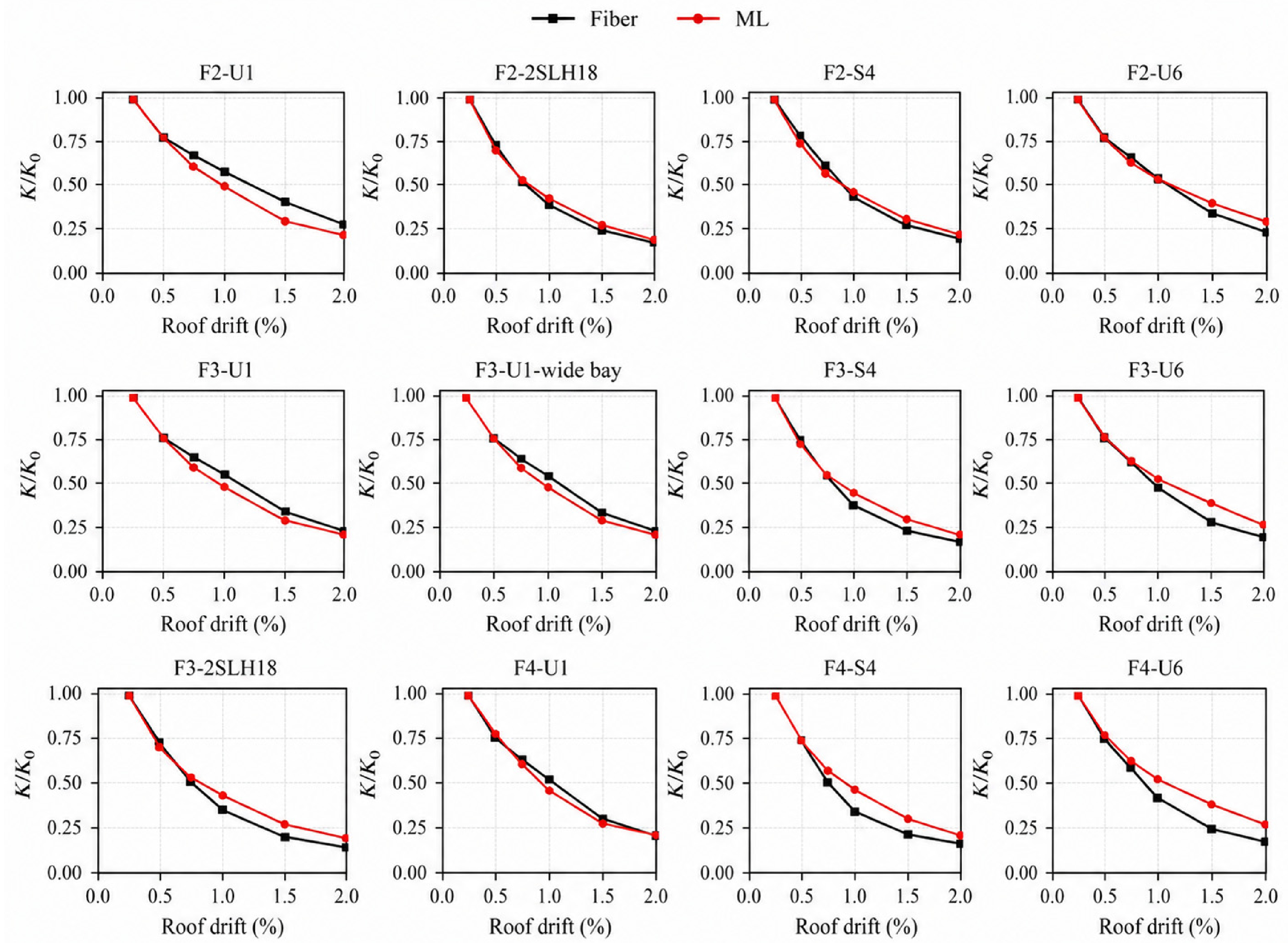
The structural stiffness-ratio trend is reproduced more consistently than the shear response. This is expected because stiffness ratio is the direct target of the degradation model, whereas shear also depends on the resulting deformation distribution. Figure 19 therefore provides the most direct frame-level comparison with the learned quantity.

Figure 19 and Table 7 quantify this distinction. Final FE/ML stiffness ratios are close for F4-U1 (0.186/0.190) but differ substantially for F4-U6 (0.157/0.256). Across the cases, stronger agreement is obtained when the learned peak-envelope deterioration and the fiber-section response evolve at comparable rates; disagreement grows when local material nonlinearity and redistribution dominate. This is also why the stiffness-ratio error is a more direct diagnostic of the learned target than shear error.

Across all 12 cases, the mean absolute structural stiffness-ratio error remains between 0.019 and 0.068, while mean shear errors span wider ranges. This ordering supports the central hypothesis that a component peak-stiffness envelope can be transferred to a reduced structural stiffness measure. It also rejects a stronger interpretation that the same reduced model is sufficient for detailed force prediction in every configuration.

The ML-updated model also captures the main story-shear distribution. Some taller frames and cases with stronger columns show overestimated upper-story shear, which indicates that equivalent stiffness updating cannot fully represent force redistribution after substantial inelasticity develops. Figure 20 shows the distributions at 2.00% roof drift.

Figure 20 further indicates that upper-story shear can be overestimated in taller or stronger-column frames. The equivalent model updates columns from story drift but enforces floor compatibility through a shear-building representation; it cannot reproduce section-by-section yielding, beam flexibility, joint deformation, or post-yield redistribution. Consequently, design variables affect accuracy through coupled mechanisms rather than a single monotonic ranking. Within the component test set, double-curvature loading and sparsely sampled short shear spans have less stable performance; at frame level, added stories and high-capacity U6-type columns expose the limitations of the structural idealization.

The grouped component results provide a second boundary check. Double-curvature specimens have a lower R² (0.8927) than double- and single-cantilever specimens, and the a/d₁ ≤ 2.0 subgroup has R² = 0.7860 but contains only four specimens. These observations identify loading configuration and short shear span as areas requiring additional data, while the comparable MAE and RMSE values caution against ranking mechanisms from R² alone in small groups.

Table 7 and Figure 17, Figure 18, Figure 19 and Figure 20 show that the framework captures the dominant structural stiffness-degradation trend and provides approximate estimates of base, story, and column shear. Agreement is strongest for stiffness ratio and less uniform for the derived shear quantities, which is consistent with the intended stiffness-based use of the method.

6.6. Benchmark Interpretation and Scope

The OpenSeesPy comparison confirms that the column-level predictions can be incorporated into a frame-level stiffness calculation under the adopted assumptions. The method is most reliable for structural stiffness-ratio degradation, while its force estimates remain approximate. It should be used as an efficient stiffness-assessment module for global degradation and demand redistribution, not as experimental validation or as a replacement for nonlinear hysteretic analysis. Moreover, direct use of member-level secant stiffness in these benchmark frames does not establish a general section-level EI transformation for arbitrary member lengths and boundary conditions.

7. Discussion

The framework passes the independently predicted $\hat{\mathrm{K}}$₀ and $\hat{\mathsf{\theta }}$_u to both the degradation and frame-level calculations. Error in $\hat{\mathrm{K}}$₀ changes the scale of absolute stiffness and force, while error in $\hat{\mathsf{\theta }}$_u shifts the normalized deformation coordinate and hence the predicted degradation state. Frame-level discrepancies also include error from the degradation model and the structural idealization. The present numerical benchmark does not allow these contributions to be separated conclusively.

The learned quantity is the cleaned peak secant stiffness envelope, not a full hysteretic constitutive response. For a specified column and historical maximum drift, the model estimates the fraction of the first-reference peak stiffness that remains. The cumulative non-negative formulation enforces a bounded, non-increasing prediction.

Repeated points at the same or nearly the same deformation are collapsed before the monotonic envelope is formed. The model therefore does not explicitly represent cycle-count effects, energy-dependent damage, or continued deterioration under repeated constant-amplitude cycles. Its state variable is best understood as a historical-maximum-drift envelope coordinate.

The comparison with constant, linear, exponential, and power-law functions shows the advantage of using specimen-specific mechanical inputs rather than one global curve. It does not determine how much of the improvement comes from the GRU, the derived indices, or the monotonic constraint. This question requires tabular ML baselines, an unconstrained sequence model, and controlled ablation studies.

At frame level, the method transfers predicted column stiffness ratios through an equivalent secant-stiffness update and calculates peak shear from V = KΔ. This formulation is transparent and consistent with the learned target, but it omits local plasticity, pinching, residual drift, energy dissipation, and a separate strength-loss law. The OpenSeesPy study should therefore be read as a benchmark of stiffness transfer and approximate demand redistribution. In addition, the reported fiber reference uses simplified elastic-beam and confinement assumptions; Table 6 summarizes the principal settings but does not constitute a complete executable input specification. Exact numerical reproduction requires the full beam properties, Concrete02 parameters, and analysis scripts. Robustness across data partitions also remains to be tested through repeated group-based splits and fully out-of-fold cascading.

In practice, the framework can serve as a rapid screening or reduced-order update module when many member configurations or peak drift states must be evaluated and full constitutive calibration is unavailable. Compared with a fiber-frame analysis, the framework uses a smaller input set and avoids fiber-level constitutive integration; it is therefore intended to reduce modeling and computational burden in screening applications. OpenSees or another detailed nonlinear analysis platform remains preferable when complete hysteresis, local damage, material strains, cyclic energy dissipation, strength loss, P–Δ effects, or collapse mechanisms are decision-critical. The two approaches are therefore complementary rather than interchangeable.

A suitable engineering workflow is therefore tiered: use the proposed model to screen many column assignments, identify stories with rapid stiffness loss, and compare peak demand-redistribution scenarios; then apply a calibrated nonlinear model to the critical configurations. This use preserves the speed and limited input burden of the proposed framework without treating it as a substitute for code acceptance checks or collapse-oriented simulation.

8. Conclusions

This study developed a hierarchical method for predicting the first-reference peak secant stiffness, drift capacity, and deformation-dependent stiffness degradation of rectangular RC columns. The predicted $\hat{\mathrm{K}}$₀ and $\hat{\mathsf{\theta }}$_u were used directly in the degradation and frame-level calculations, so the reported downstream results include scalar-model error. The main findings are:

(1) Specimen-level and peak-level datasets were constructed from the NEES/ACI 369 rectangular RC column database. A common specimen-wise split was used for all three tasks, preventing points from the same test from appearing in different data partitions.

(2) On the test set, the selected K₀ model achieved R² = 0.935, MAE = 4.098 kN/mm, and RMSE = 7.666 kN/mm. The selected θ_u model achieved R² = 0.927, MAE = 0.346 percentage points, and RMSE = 0.512 percentage points.

(3) With deformation normalized by predicted drift capacity, the cumulative sequence model achieved R² = 0.9272, MAE = 0.0542, and RMSE = 0.0788. These values include the effect of $\hat{\mathsf{\theta }}$_u error on the normalized coordinate. The non-negative cumulative formulation enforced bounded, monotonic stiffness loss.

(4) The sequence model outperformed the constant, linear, exponential, and power-law global functions. This result demonstrates the value of specimen-dependent inputs over a single degradation curve within the sampled range, but it is not an ablation of the model architecture.

(5) In the frame benchmark, mean errors ranged from 8.26% to 21.88% for base shear, 11.42% to 24.54% for story shear, and 10.19% to 23.51% for column shear. The mean absolute error in structural stiffness ratio was 0.019–0.068. Agreement was strongest for stiffness ratio and less consistent for the derived shear quantities. These results indicate numerical consistency with the adopted OpenSeesPy models rather than independent experimental validation.

(6) The frame-level procedure is an equivalent secant-stiffness assessment, not a complete hysteretic simulation. It calculates shear directly from V = KΔ and does not model unloading–reloading response, pinching, residual drift, energy dissipation, beam and joint deterioration, P–Δ effects, cycle-count deterioration, or a separate strength-degradation law. Further work is needed to quantify uncertainty and to separate errors arising from the scalar predictors, degradation model, and structural idealization.

(7) Applicability is limited to rectangular RC columns represented by the retained database ranges and to the adopted historical-maximum-drift peak-envelope and constant-axial-load frame idealizations. Corrosion is not explicitly characterized as a model variable. Explicit concrete and reinforcement strains, loading direction, cycle-count deterioration, beam/joint damage, and corrosion-related deterioration are outside the present feature and state definitions.

(8) The adopted hypotheses were supported to the extent that bounded monotonic degradation transferred coherently to structural stiffness ratios, for which mean absolute errors were 0.019–0.068. The larger and design-dependent shear errors show where the hypotheses become restrictive. The method is best used for rapid stiffness-based screening and demand-redistribution studies; OpenSees or another nonlinear platform is required when full cyclic and local response governs the assessment.

(9) The reviewers’ comments highlight clear priorities for future development: corrosion-tagged training data; harmonized concrete and reinforcement strain descriptors; signed, cycle-resolved sequences; sensitivity and ablation studies; repeated group-based validation and fully out-of-fold cascading; fully documented executable frame benchmarks with complete material and beam-property inputs; and experimental frame tests with beam, joint, P–Δ, and axial-force redistribution effects. These extensions are necessary before the method can support broader deterioration states or full seismic performance classification.