Finite Element Model Updating Based on a Physics-Constrained Sparse Response Surface

Abstract

Accurate finite element models are essential for structural condition assessment, yet nominal material properties and idealized boundary conditions can produce systematic discrepancies between numerical and measured dynamics. This study proposes a physics-constrained sparse response-surface framework that combines Elastic Net basis selection, mechanically prescribed monotonicity, adaptive sample enrichment, and identifiability-aware uncertainty assessment within a transparent finite element model-updating procedure. A scaled steel truss was tested using millimeter-wave radar, and the first three vertical natural frequencies were identified by stochastic subspace identification. The resulting sparse polynomial surrogate was independently validated before bounded inversion and ANSYS back-substitution. The mean frequency error decreased from 5.55% to 0.82%. Jacobian and bootstrap analyses further showed that several combinations of material and boundary parameters can reproduce similar modal responses, so the updated parameters are best interpreted as a coupled equivalent calibration state rather than unique direct measurements. The proposed framework therefore improves physical consistency and computational efficiency while explicitly retaining the uncertainty associated with weakly identifiable parameter directions.

1. Introduction

Finite element (FE) models provide the computational foundation for structural response prediction, damage simulation, reliability assessment, and maintenance decision-making. Their credibility, however, depends on how faithfully the numerical representation captures material properties, distributed and concentrated masses, connection flexibility, and boundary conditions. Even when structural geometry is reproduced accurately, nominal material constants and idealized supports can generate systematic discrepancies between calculated and measured modal properties. In structural health monitoring (SHM), such modelling errors are particularly consequential because they may be interpreted as damage-induced changes or may conceal the comparatively small dynamic signatures produced by actual deterioration [1,2]. FE model updating therefore constitutes an essential intermediate step between vibration measurement and model-based condition assessment.

Early model-updating approaches can broadly be divided into direct matrix-correction methods and iterative sensitivity-based methods. Direct methods modify the assembled mass or stiffness matrices so that selected measured eigenvalues, eigenvectors, and orthogonality conditions are satisfied, often through constrained matrix optimization [2,3]. Although these methods can reproduce measured modal data without repeated nonlinear optimization, the resulting matrix corrections are not always readily associated with physical material or boundary parameters, and incomplete or noisy mode shapes may produce spatially distributed changes with limited mechanical meaning. Sensitivity-based updating instead parameterizes physically interpretable quantities and linearizes modal residuals with respect to these parameters. Weighted least-square iterations are then used to reduce discrepancies in natural frequencies, mode shapes, modal assurance criteria, or frequency-response functions [3,4,5]. This approach remains one of the most established procedures in structural dynamics, but its effectiveness depends strongly on parameter selection, sensitivity-matrix conditioning, regularization, measurement completeness, and the availability of sufficiently accurate local derivatives. Repeated FE analyses may also become prohibitive when the parameter–response relationship is nonlinear, the model is large, or multiple initial points are required to avoid local minima.

Bayesian model updating provides a probabilistic alternative in which uncertain model parameters, measurement errors, and model discrepancies are represented through prior and likelihood distributions. A posterior distribution offers not only point estimates but also uncertainty intervals, parameter correlations, and evidence for competing model classes [6]. This capability is particularly valuable for ill-conditioned or non-unique inverse problems, where several parameter combinations may reproduce almost identical modal responses. Markov chain Monte Carlo (MCMC) methods are commonly used when the posterior cannot be evaluated analytically, while transitional Markov chain Monte Carlo (TMCMC) constructs a sequence of intermediate distributions between the prior and posterior to improve sampling of correlated or multimodal parameter spaces [7]. Recent tutorials have consolidated advanced sampling strategies for Bayesian model updating and emphasized that their principal limitation remains computational cost: thousands or millions of forward-model evaluations may be required for complex structures [8]. Moreover, posterior uncertainty cannot by itself eliminate structural non-identifiability if the measured responses contain insufficient independent information [9].

Metamodels, also termed surrogate models, address this computational bottleneck by approximating the mapping from uncertain FE parameters to structural responses using a limited set of high-fidelity simulations [10,11,12,13]. Kriging or Gaussian-process models are attractive because they combine flexible nonlinear approximation with a predictive variance that can guide sequential sampling [10,14]. Their accuracy, however, depends on covariance-kernel selection and hyperparameter estimation, and conventional stationary kernels may perform poorly across response surfaces whose smoothness varies strongly over the parameter domain. Radial basis function models offer flexible interpolation and are effective for irregular nonlinear surfaces, but their performance may depend sensitively on basis width, center placement, and regularization [15]. Polynomial response surfaces remain appealing for engineering inverse problems because they are inexpensive to evaluate, analytically differentiable, transparent, and straightforward to embed in bounded optimization. Their principal weakness is basis specification: low-order models may miss boundary nonlinearities, whereas complete high-order expansions introduce correlated and weakly supported terms that increase variance and produce oscillatory extrapolation. These trade-offs have motivated surrogate-assisted optimization strategies that balance global coverage, local exploitation, and the cost of additional simulations [11,12,13,14,15,16].

Recent application-oriented studies also emphasize that reliable model updating depends on a physically meaningful representation of mass, stiffness, restraints, and measured dynamic information. Nicoletti and Gara examined modelling strategies for updating infilled reinforced-concrete building FEMs, including the influence of construction-stage modelling assumptions [17], while Kurent et al. updated a seven-story cross-laminated-timber building using experimentally derived frequency-response-function modal information [18]. More recent studies have increasingly focused on improving the efficiency and uncertainty treatment of FEMU through surrogate-assisted strategies. Kamali et al. developed an inverse random-forest surrogate for deterministic structural model updating [19], Tian et al. employed Gaussian-process models to quantify natural-frequency uncertainty and update FE parameters [20], Zhang et al. combined a Gaussian-process surrogate with MCMC for Bayesian updating of a high-rise building [21], and Zhang et al. proposed a sequential surrogate framework for FEMU using incomplete modal data [22]. Together, these studies show that physically interpretable parameterization, efficient surrogate modelling, uncertainty quantification, and targeted sample enrichment are becoming increasingly interconnected in contemporary FEMU.

Sparse regression provides a principled means of controlling polynomial complexity. The least absolute shrinkage and selection operator promotes parsimonious models by shrinking weak coefficients to zero [23], while Elastic Net combines L1 and L2 penalties to retain sparsity while stabilizing groups of correlated predictors [24]. Related sparse polynomial-chaos techniques have demonstrated that significant basis terms can be selected adaptively rather than prescribed through a complete expansion [25]. More broadly, sparse identification methods have shown that interpretable governing relationships can be extracted from large candidate libraries when only a small subset of terms is dynamically relevant [26]. Nevertheless, statistical sparsity alone does not guarantee that a surrogate respects structural mechanics. A polynomial can fit sampled frequencies accurately while violating known response directions between samples, for example, predicting an increase in natural frequency as equivalent density increases under otherwise fixed conditions.

This limitation reflects a wider transition from purely data-fitted models toward physics-informed learning. Physics-informed neural networks incorporate governing equations or constitutive residuals into training objectives [27], while physics-informed machine learning more generally embeds conservation laws, symmetries, admissibility conditions, or qualitative physical trends into model architectures and optimization procedures [28]. Such methods can improve data efficiency and physical plausibility, but highly parameterized neural representations may remain unnecessarily complex for low-dimensional FE updating, and their optimization can be difficult to diagnose. For problems involving a small number of uncertain physical parameters, an explicit sparse response surface with mechanically motivated inequality constraints offers a more transparent alternative: it retains analytical derivatives and coefficient-level interpretability while preventing physically inadmissible trends.

Surrogate-based FEMU still faces two practical issues: maintaining adequate accuracy near the inverse-solution region with a limited number of FE analyses and avoiding non-physical surrogate trends or weakly identifiable parameter combinations. Surrogate quality should therefore be assessed using independent prediction errors, physical consistency, and parameter identifiability [8,9,29].

Interferometric radar enables non-contact vibration measurement at multiple structural targets [30,31,32,33]. In practical applications, line-of-sight projection and the correspondence between radar targets and FE degrees of freedom can affect modal interpretation. This motivates combining radar-derived modal information with FE model updating that explicitly accounts for modelling uncertainty.

The present study develops a physics-constrained sparse response-surface procedure and evaluates it using modal frequencies identified from millimeter-wave radar measurements of a scaled steel truss. An initial FE sample database was used to construct sparse polynomial surrogates through Elastic Net regularization and hierarchical term retention, after which mechanically admissible monotonicity conditions were imposed on the modal responses. The surrogate was then sequentially enriched by selecting simulations that balanced predictive uncertainty, proximity to the measured target, and coverage of the existing parameter space. A local residual correction was introduced only when cross-validation demonstrated a reproducible reduction in prediction errors. The resulting surrogate was evaluated on an independent test set before being used for bounded parameter inversion and FE back-substitution. Finally, local Jacobian analysis and bootstrap resampling were employed to assess parameter identifiability and quantify the uncertainty of the updated solution.

2. Methodology

The proposed finite element model-updating framework uses experimentally identified modal frequencies to calibrate a parameterized FE model through a physics-constrained surrogate. First, a parameterized ANSYS 14.5 model is established and sampled within the prescribed ranges of equivalent density, elastic modulus, and support stiffness to generate the FE response database. The initial samples are used to construct third-order sparse polynomial response surfaces, in which Elastic Net regularization controls that model complexity and monotonicity constraints enforce physically admissible parameter-frequency trends. Adaptive enrichment is then used to add samples in regions that are both uncertain and relevant to the inverse solution, while a cross-validation gate determines whether an additional local residual correction is justified. After the surrogate accuracy is verified on an independent test set, the measured modal frequencies are used as targets for bounded parameter inversion. The identified parameters are finally substituted back into the original ANSYS model for FE-level verification, and Jacobian/SVD analysis, together with bootstrap resampling, is used to evaluate parameter identifiability and uncertainty.

2.1. Experimental Setup and Baseline FE Model

A scaled main truss derived from the steel roof of a large sports venue was constructed for the experimental investigation. The model had a span of 5.5 m and a height of approximately 0.2 m. Different member groups used geometric scales of approximately 1:10–1:20 to retain the main load-transfer topology while remaining practical for laboratory fabrication. The specimen used gusset-plate bolted connections, and the undamaged configuration served as the modal baseline. The connection components were physically present but were not all represented as separate solid parts in the beam-element FE model.

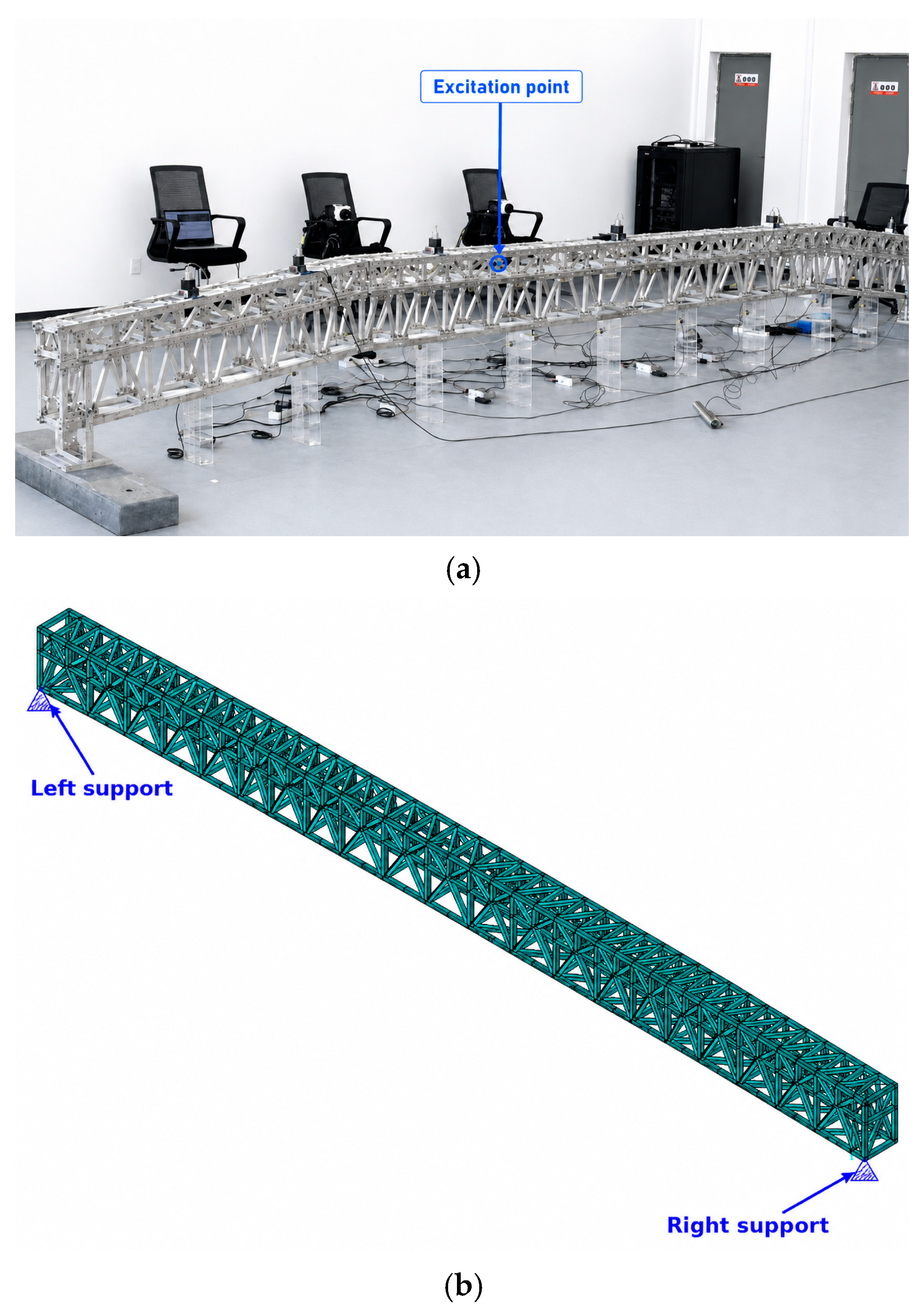
Dynamic vibration tests were conducted on 15 December 2024 using eight response points along the truss and one ground reference point. An INV 9314 impact force bar (Beijing Oriental Institute of Vibration and Noise, Beijing, China) was used to apply impulse excitation directly to the truss. The excitation point was kept fixed throughout the modal tests and is indicated in Figure 1a. Acceleration responses were recorded using the 941B vibration acquisition system at 500 Hz, low-pass filtered at 200 Hz, and recorded for no less than 30 s for each test. The millimeter-wave radar measured line-of-sight displacement from selected targets fitted with corner reflectors, while Panasonic HG-C1050 laser displacement sensors (Panasonic Corporation, Osaka, Japan) at corresponding target locations provided an independent displacement reference. The radar and laser displacement measurements showed a mean deviation of 0.03 mm. The radar-derived vibration responses were processed using stochastic subspace identification (SSI), yielding the first three radar-identified vertical natural frequencies of 11.72, 51.21, and 122.42 Hz.

The identified modal information was used to update a parameterized ANSYS model. The steel members were modelled with the three-dimensional two-node beam element BEAM188, concentrated dead loads with MASS21, and vertical support flexibility with COMBIN14. In the adopted three-dimensional BEAM188 formulation, each member node retained the six structural degrees of freedom UX, UY, UZ, ROTX, ROTY, and ROTZ. MASS21 supplied concentrated translational inertia, while COMBIN14 acted in the vertical translational degree of freedom at the two physical end supports indicated in Figure 1b; the remaining support restraints were imposed through nodal boundary conditions. Member centerlines followed the physical joint nodes, so joint coordinates and member connectivity defined the principal discretization. Before generation of the FE database, the joint coordinates, connectivity, element formulation, section properties, mass assignment, and support implementation were checked and then kept consistent for all analyses. These checks follow the numerical-verification principle adopted in [34]. Only the vertical dynamic characteristics corresponding to the measured modes were used in the updating procedure. The parameter-dependent equation of motion is

$$\mathrm{M}\left(\mathsf{\theta }\right)\ddot{\mathrm{u}}\left(\mathrm{t}\right)+\mathrm{C}\left(\mathsf{\theta }\right)\dot{\mathrm{u}}\left(\mathrm{t}\right)+\mathrm{K}\left(\mathsf{\theta }\right)\mathrm{u}\left(\mathrm{t}\right)=\mathrm{F}\left(\mathrm{t}\right)$$

(1)

where M, C, and K are the mass, damping, and stiffness matrices, respectively; u is the displacement vector; F is the external load vector; and $\theta$ is the physical parameter vector. For undamped free vibration, the eigenproblem and frequency relation are

$$\left[\mathbf{K}\left(\mathsf{\theta }\right)-{\omega }_i^2\mathbf{M}\left(\mathsf{\theta }\right)\right]{\mathsf{\varphi }}_i=0, f_i={\displaystyle \frac{{\omega }_i}{2\pi }}$$

(2)

The updating vector was defined as $\theta ={[\rho ,\mathrm{E},\kappa ]}^T$, where $\rho$ is equivalent density, E is equivalent elastic modulus, and $\kappa ={\log }_{10}(K_y)$ is the logarithm of the vertical support stiffness, as shown in

Table 1. Updating parameters and prescribed physical trends.

Parameter	Range	Unit	Primary Effect	Expected Trend
Equivalent density, $\rho$	7600–8100	kg/m3	Mass matrix	Frequency decreases
Equivalent elastic modulus, E	190–215	GPa	Structural stiffness	Frequency increases
Support stiffness logarithm, $\kappa$ = log10(Ky)	7–10	-	Boundary stiffness	Frequency increases

. The logarithmic transformation prevents the high-stiffness end of the multi-order-of-magnitude range from dominating the numerical scale.

2.2. Sample Design and Data Partition

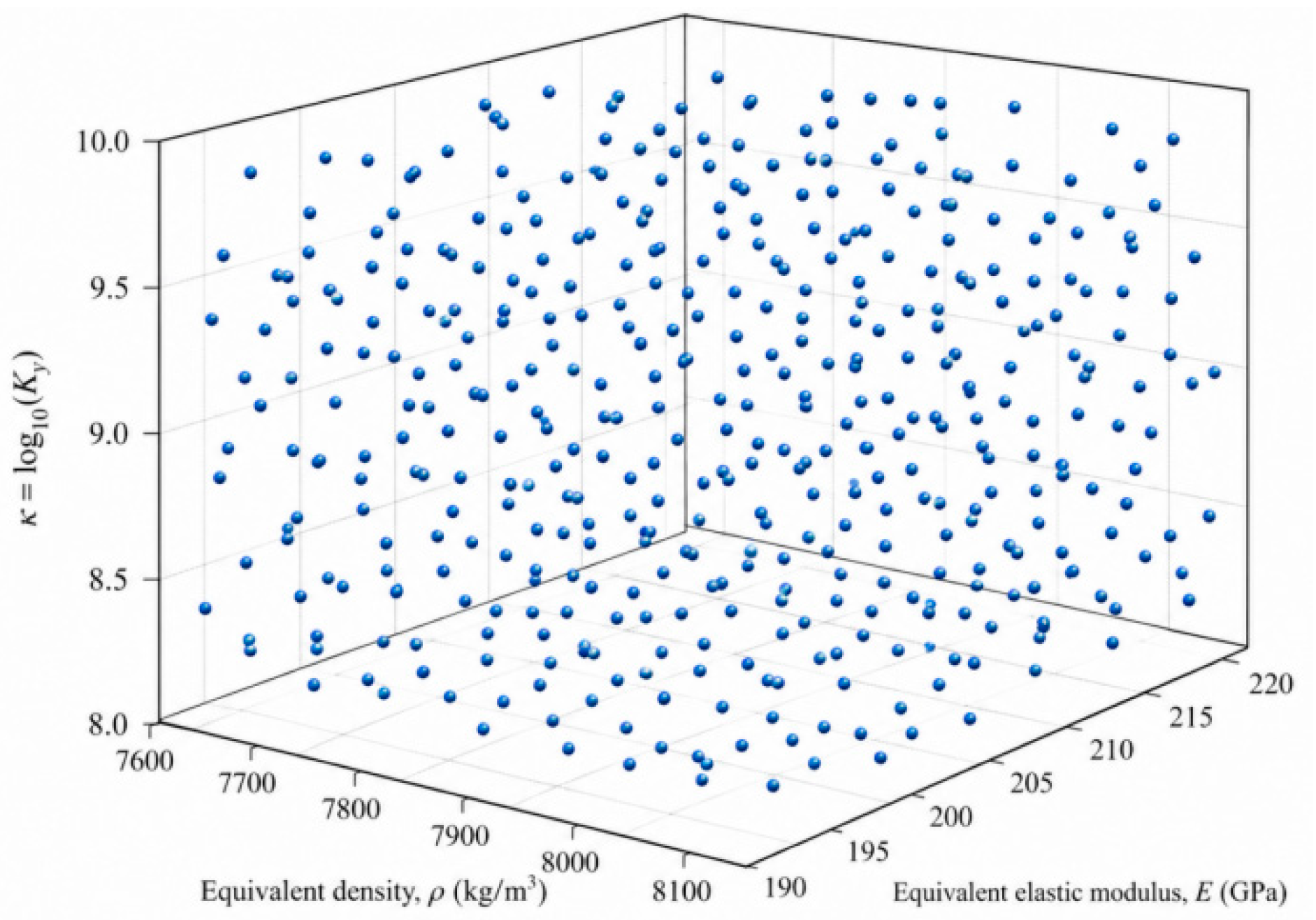
A maximin Latin hypercube sampling design was employed to achieve broad marginal coverage while minimizing local clustering. The physical variables were mapped onto the common interval [−1, 1] according to

$$x_j=2{\displaystyle \frac{{\theta }_j-{\theta }_{j,\mathrm{L}}}{{\theta }_{j,\mathrm{U}}-{\theta }_{j,\mathrm{L}}}}-1, j=1,2,3$$

(3)

As shown in Figure 2 and

Table 2. Descriptive statistics of the 200 finite element samples.

Variable	Minimum	Maximum	Mean	Standard Deviation
$\rho$ (kg/m3)	7600.5480	8099.5520	7850.0488	144.7974
E (GPa)	190.0516	214.9219	202.5033	7.2334
$\kappa$	7.0146	9.9982	8.4999	0.8682
f1 (Hz)	10.6960	12.2959	11.5840	0.3239
f2 (Hz)	39.3183	54.4890	49.7965	3.9346
f3 (Hz)	106.7005	127.3015	118.6076	4.5553

, a total of 200 ANSYS modal analyses were available. The 140 initial samples were used to construct and tune the global surrogate. Of the remaining 60 candidates, 30 were added over six adaptive-enrichment rounds and 30 were retained as an untouched independent test set. The 30 test samples were reserved exclusively for final evaluation, and the minimum and mean nearest-neighbor distances in the normalized space were 0.0247 and 0.1036, respectively. This 140/30/30 partition separates model construction, adaptive refinement, and final validation, while the 200-point maximin design provides systematic coverage of the prescribed parameter domain [35].

2.3. Physics-Constrained Sparse Response Surface Construction

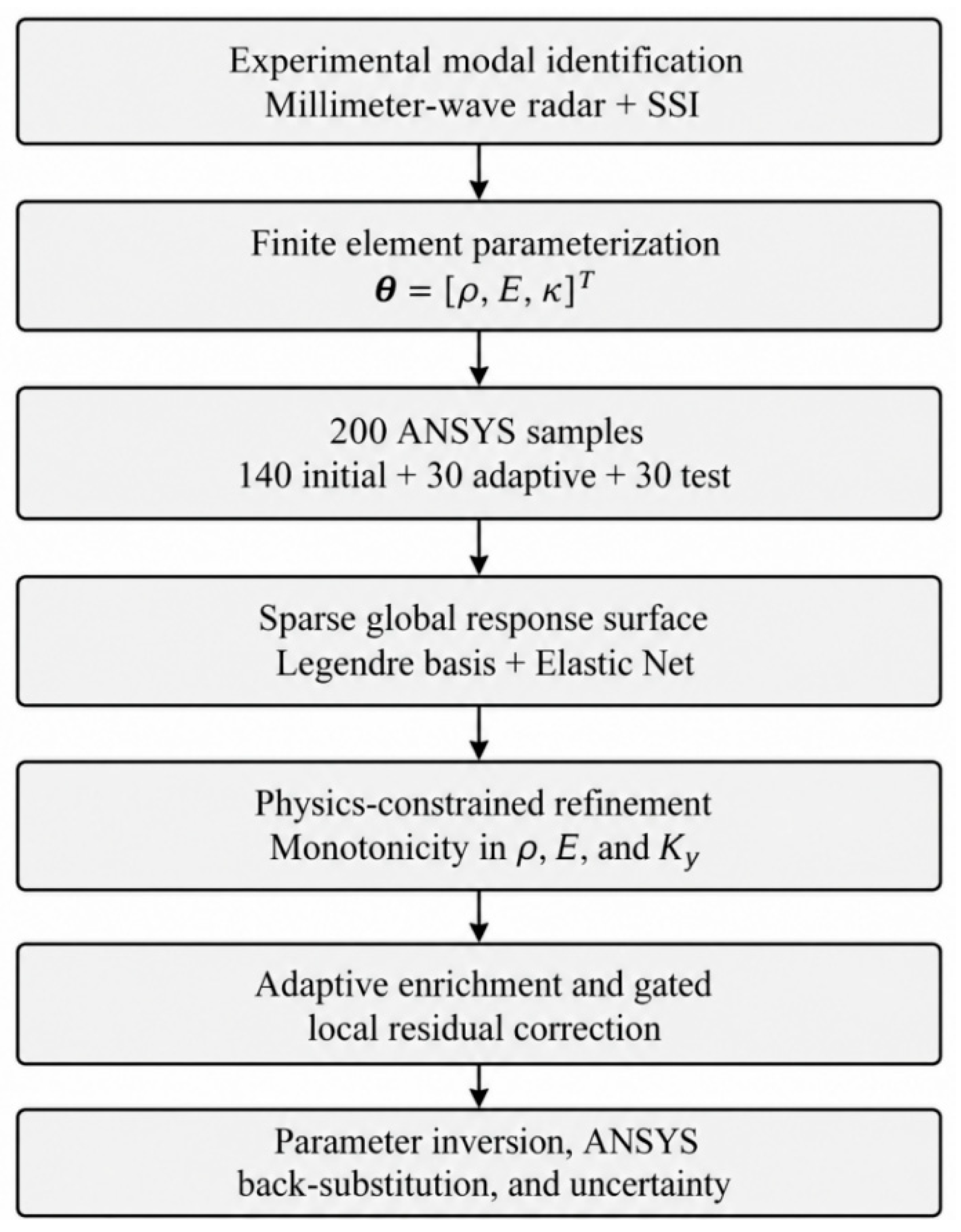
Figure 3 summarizes the model-updating workflow. The radar-identified natural frequencies obtained from the experiment described in Section 2.1 were used as the updating targets [36]. A parameterized ANSYS model supplied the initial database for sparse polynomial response surfaces with Elastic Net selection, hierarchical term retention, and monotonicity constraints. The surrogates were then refined by adaptive enrichment and, where supported by cross-validation, local residual correction. After independent test-set validation, the final surrogate was used for bounded inversion, ANSYS back-substitution, Jacobian-based identifiability analysis, and bootstrap uncertainty quantification.

Third-order Legendre polynomials were used because their orthogonality on [−1, 1] reduces collinearity among high-order terms. Let x = T(θ) = [x₁,x₂,x₃]^T denote the normalized input. The tensor-product basis is

$${\mathsf{\Psi }}_{\mathsf{\alpha }}\left(\mathrm{x}\right)={\displaystyle {\prod }_{\mathrm{j}=1}^3}{\mathrm{P}}_{{\mathsf{\alpha }}_{\mathrm{j}}}\left({\mathrm{x}}_{\mathrm{j}}\right), \mathsf{\alpha }\in {\mathcal{A}}_3$$

(4)

where α = [α₁,α₂,α₃]^T is a multi-index, and A₃ contains all nonconstant terms with a total degree from one to three. For three variables, this gives 19 penalized candidate terms. A separate intercept is retained and is not penalized. The response surface for the modal order, r, is

$${\hat{\mathrm{f}}}_{\mathrm{r}}\left(\mathrm{x}\right)={\mathsf{\beta }}_{\mathrm{r},0}+{\sum }_{\mathsf{\alpha }\in {\mathcal{A}}_3}{\mathsf{\beta }}_{\mathrm{r},\mathsf{\alpha }}{\mathsf{\Psi }}_{\mathsf{\alpha }}\left(\mathrm{x}\right), \mathrm{r}=\mathrm{1,2},3$$

(5)

For each modal frequency, the complete 19-term candidate model was first fitted by Elastic Net [24]. Candidate selection therefore occurred during, rather than before, the penalized fitting process. The coefficients were obtained from

$$\begin{array}{rr}\left({\hat{\mathsf{\beta }}}_{\mathrm{r},0},{\hat{\mathsf{\beta }}}_{\mathrm{r}}\right)=\underset{{\mathsf{\beta }}_{\mathrm{r},0},{\mathsf{\beta }}_{\mathrm{r}}}{\mathrm{a}\mathrm{r}\mathrm{g} \mathrm{m}\mathrm{i}\mathrm{n}}\{& {\displaystyle \frac{1}{\mathrm{N}}}{\displaystyle {\sum }_{\mathrm{n}=1}^{\mathrm{N}}}{\left[{\mathrm{y}}_{\mathrm{r},\mathrm{n}}-{\mathsf{\beta }}_{\mathrm{r},0}-\mathsf{\varphi }{\left({\mathrm{x}}^{\left(\mathrm{n}\right)}\right)}^{\mathrm{T}}{\mathsf{\beta }}_{\mathrm{r}}\right]}^2+\mathsf{\lambda }\left[\mathsf{\eta }\parallel {\mathsf{\beta }}_{\mathrm{r}}{\parallel }_1+{\displaystyle \frac{1-\mathsf{\eta }}{2}}\parallel {\mathsf{\beta }}_{\mathrm{r}}{\parallel }_2^2\right]\}\\ & \end{array}$$

(6)

The mixing parameter, η, controls the proportion of the L1 penalty, while λ controls the overall regularization strength. For fixed (λ,η), minimizing Equation (6) balances fitting errors, sparsity, and coefficient stability. The tuning pair was selected by five-fold cross-validation on the 140 initial samples: each of the five subsets was used once as a 28-sample validation fold, while the other 112 samples fitted the model. The mean validation error was

$${\mathrm{M}\mathrm{S}\mathrm{E}}_{\mathrm{C}\mathrm{V},\mathrm{r}}\left(\mathsf{\lambda },\mathsf{\eta }\right)={\displaystyle \frac{1}{5}}{\displaystyle {\sum }_{\mathrm{k}=1}^5}{\displaystyle \frac{1}{\left|{\mathrm{V}}_{\mathrm{k}}\right|}}{\sum }_{\mathrm{n}\in {\mathrm{V}}_{\mathrm{k}}}{\left[{\mathrm{y}}_{\mathrm{r},\mathrm{n}}-{\hat{\mathrm{y}}}_{\mathrm{r},\mathrm{n}}^{\left(-\mathrm{k}\right)}\left(\mathsf{\lambda },\mathsf{\eta }\right)\right]}^2$$

(7)

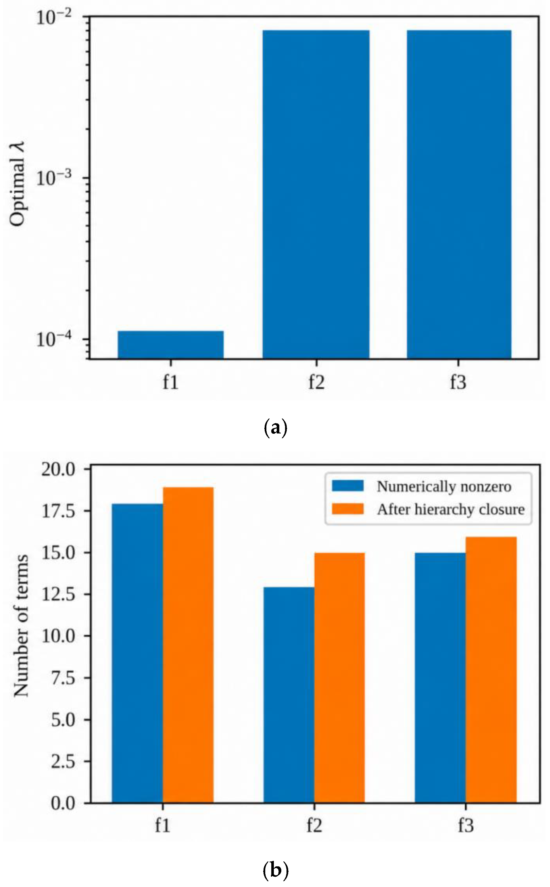
After the optimal pair was determined, the Elastic Net model was refitted using all 140 samples. As shown in

Table 3. Elastic Net tuning and sparse-term selection.

Mode	Optimal η	Optimal λ	Candidate Terms	Nonzero Terms	Terms After Closure
f1	1.0000	9.1030 × 10−5	19	18	19
f2	1.0000	8.2864 × 10−3	19	13	15
f3	1.0000	8.2864 × 10−3	19	15	16

and Figure 4, terms with an absolute coefficient larger than 1 × 10⁻⁸ were regarded as numerically nonzero. Strong hierarchy was then enforced: when an interaction or high-order term was retained, its required lower-order parent terms were also included. This closure facilitates stable interpretation and prevents isolated high-order effects. The 1 × 10⁻⁸ cutoff is therefore only a numerical-zero criterion used to remove floating-point remnants after regularized fitting; it is not an additional physical-significance threshold.

The sparse term set was fixed before the final coefficient refinement. Mechanical knowledge was imposed at the response level rather than by assigning signs to individual polynomial coefficients. For all three modal responses, the admissible local trends were

$${\displaystyle \frac{\partial {\hat{\mathrm{f}}}_{\mathrm{r}}}{\partial \mathsf{\rho }}}\le 0, {\displaystyle \frac{\partial {\hat{\mathrm{f}}}_{\mathrm{r}}}{\partial \mathrm{E}}}\ge 0, {\displaystyle \frac{\partial {\hat{\mathrm{f}}}_{\mathrm{r}}}{\partial \mathsf{\kappa }}}\ge 0$$

(8)

The derivative signs were checked for the modelling samples and at 80 additional points distributed in the normalized parameter domain. Squared violations were added to the regression objective:

$${\mathcal{L}}_{\mathrm{r}}={\displaystyle \frac{1}{\mathrm{N}}}\parallel {\mathrm{y}}_{\mathrm{r}}-{\mathsf{\beta }}_{\mathrm{r},0}1-{\mathsf{\Phi }}_{\mathrm{r}}{\mathsf{\beta }}_{\mathrm{r}}{\parallel }_2^2+{\mathsf{\lambda }}_{\mathrm{m}}{\mathcal{L}}_{\mathrm{m}\mathrm{o}\mathrm{n}\mathrm{o},\mathrm{r}}+{\mathsf{\lambda }}_2\parallel {\mathsf{\beta }}_{\mathrm{r}}{\parallel }_2^2$$

(9)

Here Φ_r is the design matrix associated with the fixed sparse term set, Lmono; r is the monotonicity-violation penalty; λ_m controls physical enforcement; and λ₂ provides mild coefficient stabilization. The constrained solution preserves the sparse polynomial structure while suppressing nonphysical local reversals.

2.4. Adaptive Enrichment and Gated Local Correction

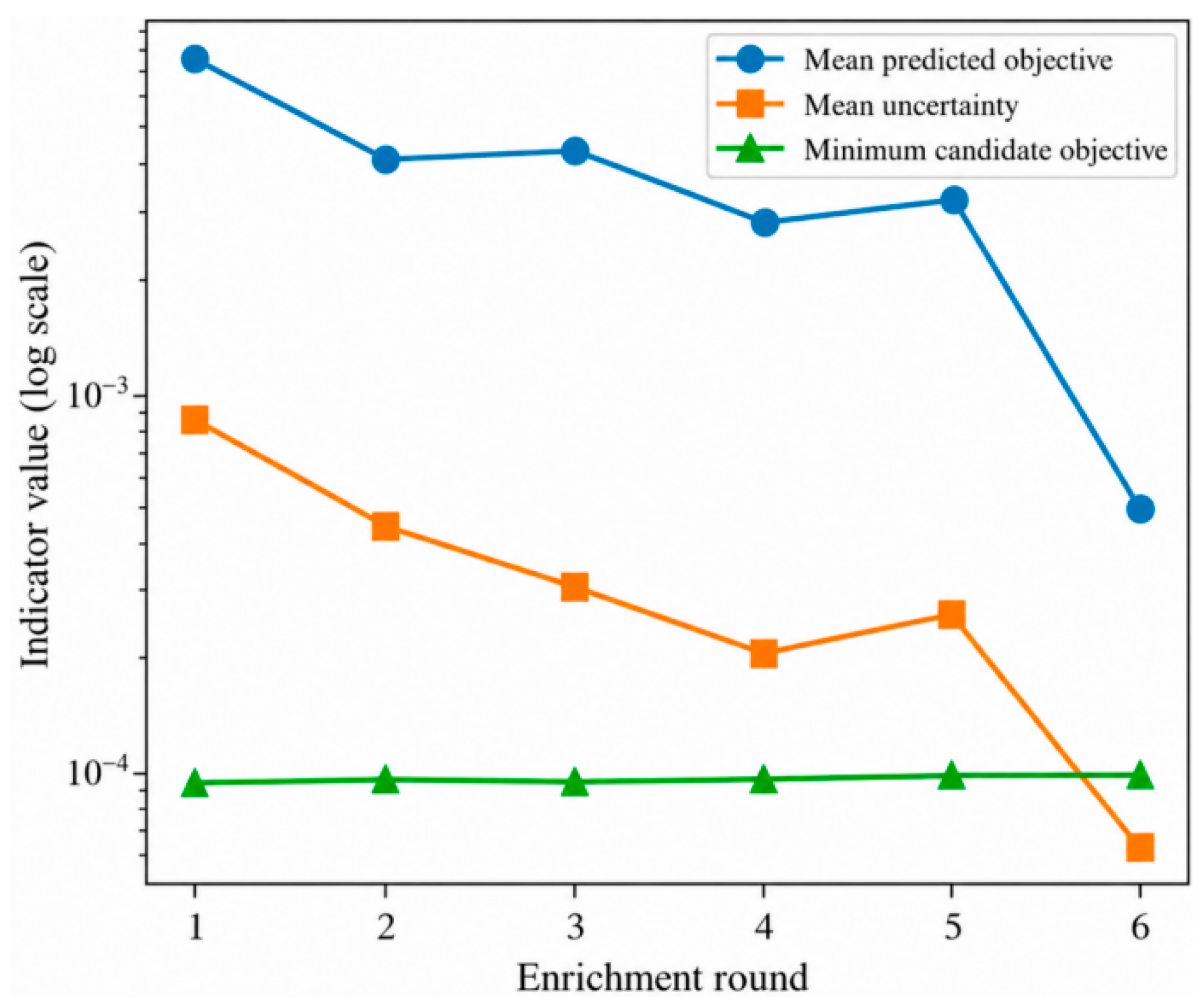
The initial global model was updated iteratively. In every round, bootstrap resampling of the current modelling set produced multiple surrogate models. At a candidate point, their objective-function predictions yielded a mean and a standard deviation, ${\sigma }_J$, which quantified surrogate uncertainty. Candidate points were ranked by

$$\mathcal{A}\left({\mathrm{x}}^{\left(\mathrm{c}\right)}\right)=0.45{\tilde{\mathsf{\sigma }}}_{\mathrm{J}}\left({\mathrm{x}}^{\left(\mathrm{c}\right)}\right)+0.40\left[1-\tilde{\mathrm{J}}\left({\mathrm{x}}^{\left(\mathrm{c}\right)}\right)\right]+0.15{\tilde{\mathrm{d}}}_{\mathrm{m}\mathrm{i}\mathrm{n}}\left({\mathrm{x}}^{\left(\mathrm{c}\right)}\right)$$

(10)

The three normalized components favor uncertain locations, low predicted objective values, and points distant from existing samples. The weights 0.45, 0.40, and 0.15 prioritize uncertainty and the anticipated updating region while preserving space-filling behavior. The weights were used as fixed empirical priority coefficients rather than as theoretically optimal constants. Their relative magnitudes reflect the purpose of the present enrichment stage: improving surrogate resolution in regions that are both uncertain and potentially relevant to the inverse solution. Therefore, the uncertainty and target-relevance components were assigned the dominant weights of 0.45 and 0.40, respectively, while a smaller but nonzero weight of 0.15 was retained for space filling to avoid excessive clustering. Five candidates were selected per round; their existing ANSYS responses were added to the modelling set, the global response surfaces were refitted, and all indicators were recomputed. Six rounds produced 30 adaptive samples.

$${\mathsf{\sigma }}_{\mathrm{J}}\left({\mathrm{x}}^{\left(\mathrm{c}\right)}\right)={\left\{{\displaystyle \frac{1}{\mathrm{B}-1}}{\displaystyle {\sum }_{\mathrm{b}=1}^{\mathrm{B}}}{\left[{\mathrm{J}}^{\left(\mathrm{b}\right)}\left({\mathrm{x}}^{\left(\mathrm{c}\right)}\right)-\overline{\mathrm{J}}\left({\mathrm{x}}^{\left(\mathrm{c}\right)}\right)\right]}^2\right\}}^{1/2}$$

(11)

A local quadratic model was fitted to the residuals of the global response surface in the enhanced region, defined here as the portion of the normalized domain represented by the adaptively selected target-relevant samples. No additional boundary parameter was tuned for this region. Because local residual fitting can amplify random errors, its contribution was controlled by a gate:

$${\hat{\mathrm{f}}}_{\mathrm{r}}^{\mathrm{f}\mathrm{i}\mathrm{n}\mathrm{a}\mathrm{l}}\left(\mathrm{x}\right)={\hat{\mathrm{f}}}_{\mathrm{r}}^{\mathrm{G}}\left(\mathrm{x}\right)+{\mathsf{\alpha }}_{\mathrm{r}}\mathrm{w}\left(\mathrm{x}\right){\hat{\mathrm{e}}}_{\mathrm{r}}\left(\mathrm{x}\right)$$

(12)

As shown in Figure 5 and

Table 4. Cross-validation results for the local residual gate.

Mode	Optimal Gate αr	CV-MSE at αr = 0	Minimum CV-MSE
f1	0.25	6.9971 × 10−5	6.8353 × 10−5
f2	0	0.2435	0.2435
f3	0	0.2470	0.2470

, the gate, αr, was searched from 0 to 1 in increments of 0.05 and selected by five-fold cross-validation. A value of zero disables the local correction. The first-mode gate was 0.25, whereas the second- and third-mode gates were zero; thus, the method accepted the local model only where its improvement was reproducible.

2.5. Model-Updating Strategy and Uncertainty Quantification

The target was the vector of radar-identified frequencies f_m = [11.72, 51.21, 122.42]^T Hz. Equal weighting of the three relative frequency errors prevented the numerically larger third frequency from dominating the inversion. The updating problem was

$$\mathrm{J}\left(\mathsf{\theta }\right)={\displaystyle \frac{1}{3}}{\displaystyle {\sum }_{\mathrm{i}=1}^3}{\left[{\displaystyle \frac{{\hat{\mathrm{f}}}_{\mathrm{i}}\left(\mathcal{T}\left(\mathsf{\theta }\right)\right)-{\mathrm{f}}_{\mathrm{i}}^{\mathrm{m}}}{{\mathrm{f}}_{\mathrm{i}}^{\mathrm{m}}}}\right]}^2, {\mathsf{\theta }}^{*}=\underset{{\mathsf{\theta }}_{\mathrm{L}}\le \mathsf{\theta }\le {\mathsf{\theta }}_{\mathrm{U}}}{\mathrm{a}\mathrm{r}\mathrm{g} \mathrm{m}\mathrm{i}\mathrm{n}}\mathrm{J}\left(\mathsf{\theta }\right)$$

(13)

A total of 6000 random points were screened over the bounded parameter domain, and the ten lowest-objective points were used to initialize bound-constrained L-BFGS-B searches. The smallest converged objective was retained. Because the screening and multi-start searches evaluated the explicit surrogate rather than ANSYS, their additional computational cost was negligible.

The final surrogate was assessed only on the 30 held-out samples. The principal dimensional metric was the root mean square error

$${\mathrm{R}\mathrm{M}\mathrm{S}\mathrm{E}}_{\mathrm{r}}={\left[{\displaystyle \frac{1}{{\mathrm{N}}_{\mathrm{t}}}}{\displaystyle {\sum }_{\mathrm{n}=1}^{{\mathrm{N}}_{\mathrm{t}}}}{\left({\mathrm{y}}_{\mathrm{r},\mathrm{n}}-{\hat{\mathrm{y}}}_{\mathrm{r},\mathrm{n}}\right)}^2\right]}^{1/2}$$

(14)

Together with RMSE, the coefficient of determination (R²), mean absolute percentage error (MAPE), and maximum absolute relative error (MaxARE) were reported. The staged comparison among the 140-sample global model, the 170-sample enhanced model, and the final gated model separated the effects of adaptive enrichment from those of local correction.

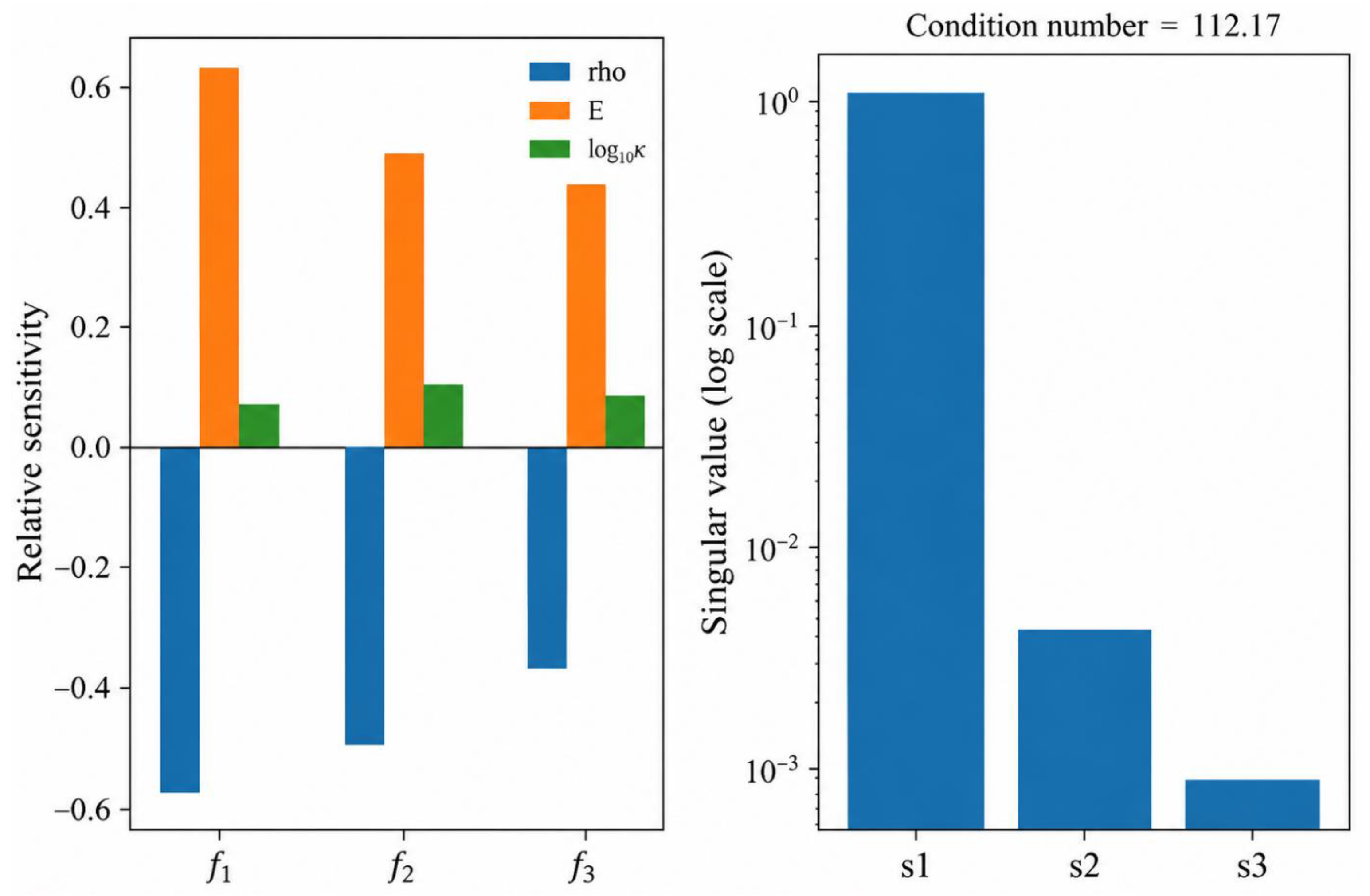
A low frequency-matching objective does not by itself guarantee unique parameters. The local relative-sensitivity matrix was calculated by centered finite differences at the optimum:

$${\mathrm{S}}_{\mathrm{i}\mathrm{j}}\left({\mathsf{\theta }}^{*}\right)={\displaystyle \frac{{\mathsf{\theta }}_{\mathrm{j}}^{*}}{{\mathrm{f}}_{\mathrm{i}}\left({\mathsf{\theta }}^{*}\right)}}{{\displaystyle \frac{\partial {\mathrm{f}}_{\mathrm{i}}}{\partial {\mathsf{\theta }}_{\mathrm{j}}}}|}_{\mathsf{\theta }={\mathsf{\theta }}^{*}}$$

(15)

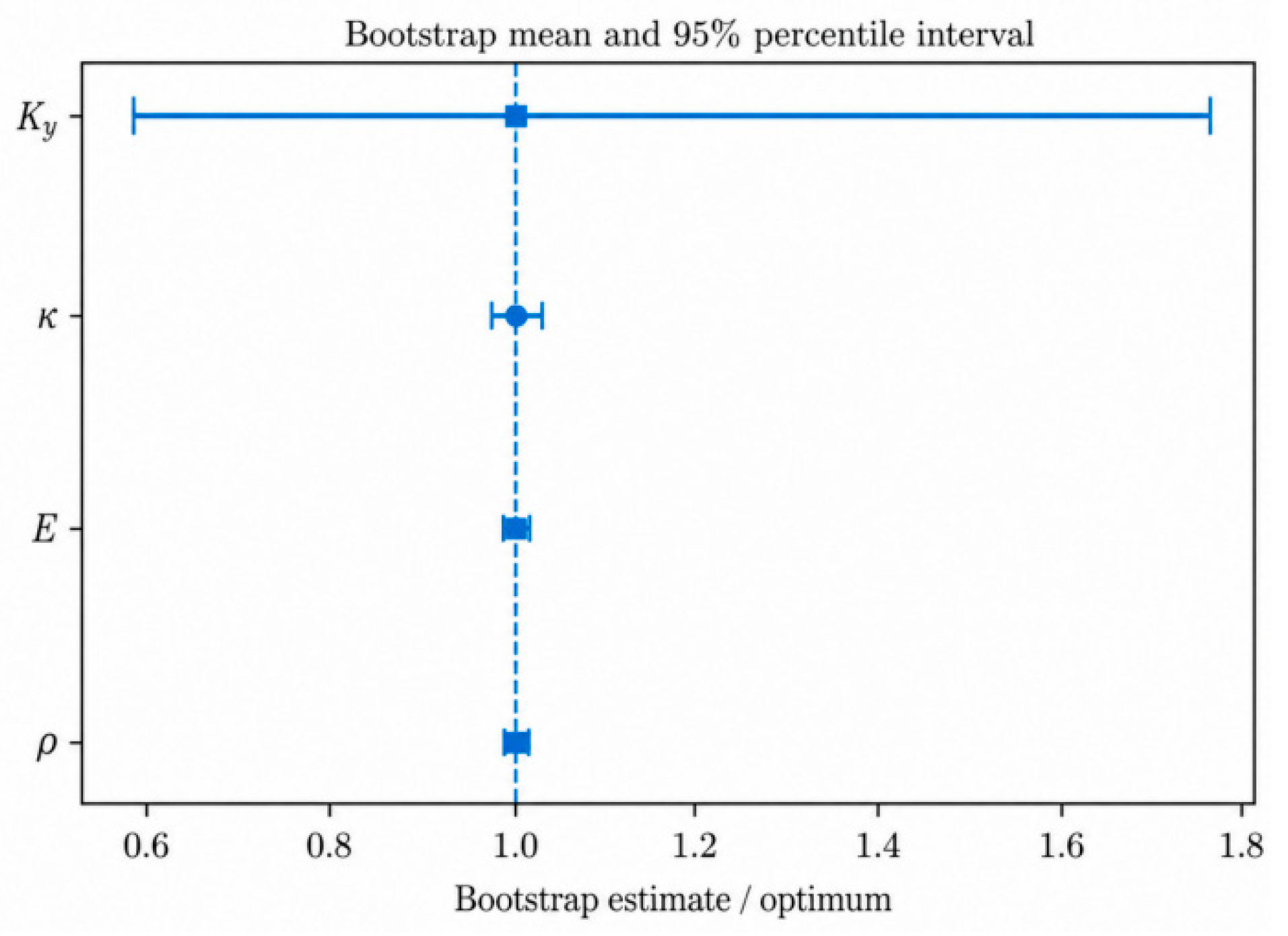
Singular-value decomposition of this normalized Jacobian quantified weak parameter directions. In addition, B = 100 bootstrap datasets were drawn with replacement from the 170 modelling samples, while the selected polynomial structure was kept fixed. This number was used as a practical balance between repeated surrogate refitting and stable percentile summaries for the present low-dimensional problem. Each bootstrap sample was refitted and re-inverted from starting points perturbed within the prescribed parameter bounds. The percentile interval was

$${\mathrm{C}\mathrm{I}}_{95\%}\left({\mathsf{\theta }}_{\mathrm{j}}^{*}\right)=\left[{\mathrm{Q}}_{0.025}\left(\{{\mathsf{\theta }}_{\mathrm{j},\mathrm{b}}^{*}{\}}_{\mathrm{b}=1}^{\mathrm{B}}\right),\hspace{0.17em}{\mathrm{Q}}_{0.975}\left(\{{\mathsf{\theta }}_{\mathrm{j},\mathrm{b}}^{*}{\}}_{\mathrm{b}=1}^{\mathrm{B}}\right)\right]$$

(16)

3. Results

3.1. Parameter-Frequency Characteristics

This subsection first examines the FE sample database to establish the parameter-frequency trends used to interpret the surrogates. The 200-sample database exhibited clear but mode-dependent relationships. Equivalent density was negatively correlated with all frequencies and most strongly with f₁. Equivalent modulus had a Pearson correlation of 0.8348 with f₁. The support-stiffness logarithm was the dominant simple correlate of f₂ and f₃, with Pearson coefficients of 0.7727 and 0.8110, as shown in Figure 6.

3.2. Surrogate Accuracy and Effect of Adaptive Enrichment

The independent test set was then used to evaluate surrogate accuracy and the effect of adaptive enrichment. All three modes selected η = 1. The first-mode regularization retained all 19 nonconstant terms after hierarchical closure. The second and third modes retained 15 and 16 terms, respectively.

As shown in

Table 5. Independent-test performance of the initial, enhanced, and final surrogates.

Mode	140 R2	170 R2	Final R2	MAPE (%)	MaxARE (%)
f1	0.9987	0.9988	0.9988	0.0641	0.2674
f2	0.9447	0.9496	0.9496	0.6643	1.9849
f3	0.9881	0.9902	0.9902	0.2144	0.5669

, the final R² values were 0.9988, 0.9496, and 0.9902. The MaxARE of the second mode was 1.9849%.

3.3. Updated Parameters and ANSYS Back-Substitution

The identified parameter vector was subsequently returned to the original ANSYS model for FE-level verification. The response-surface inversion yielded the parameters listed in

Table 6. Parameters obtained from response-surface inversion.

Parameter	Updated Value	Unit
$\rho$	7988.0954	kg/m3
E	204.8769	GPa
$\kappa$ = log10(Ky)	9.7473	-
Ky	5.5889 × 109	N/m

. As shown in

Table 7. Measured, initial, and updated ANSYS frequencies and experimental-FE MAC values.

Mode	Measured (Hz)	Initial FE (Hz)	Updated FE (Hz)	Initial Error (%)	Updated Error (%)	Initial MAC (%)	Updated MAC (%)
1	11.7200	12.9500	11.8600	10.4949	1.1945	94.5	95.2
2	51.2100	53.1100	51.5600	3.7102	0.6835	93.7	94.1
3	122.4200	125.4300	123.1300	2.4587	0.5800	92.2	90.8
Mean	-	-	-	5.5546	0.8193	93.5	93.4

and Figure 7, ANSYS back-substitution gave 11.86, 51.56, and 123.13 Hz. The corresponding errors decreased from 10.49%, 3.71%, and 2.46% to 1.19%, 0.68%, and 0.58%, respectively, and the mean relative error decreased from 5.55% to 0.82%. Table 7 also reports experimental-FE MAC values in percentages. The first two modes increased slightly from 94.5% and 93.7% to 95.2% and 94.1%, while the third decreased from 92.2% to 90.8% but remained above 90%. Because MAC was not included in the updating objective, improvements in every mode-shape correlation were not imposed.

3.4. Identifiability and Bootstrap Uncertainty

Finally, parameter identifiability was examined to determine whether the low frequency error corresponded to a well-constrained parameter solution. At the optimum, the relative sensitivities (

Table 8. Relative sensitivities at the optimum.

Parameter	f1	f2	f3
$\rho$	−0.6628	−0.5752	−0.5049
E	0.6486	0.5495	0.5062
$\kappa$	0.0716	0.1069	0.0922

) reveal a clear compensation pattern: density and elastic modulus exhibit nearly equal magnitudes but opposite signs across all three modes, whereas the support-stiffness logarithm shows much smaller local sensitivities. The objective-function surface in the E-$\kappa$ plane (Figure 8) confirms this structure, displaying an elongated valley that indicates weak sensitivity to support stiffness near the optimum.

Singular value decomposition of the normalized Jacobian yields values of 1.4239, 0.0383, and 0.0127, resulting in a condition number of 112.17 (Figure 9). The two-order-of-magnitude gap between the largest and smallest singular values identifies a weakly identifiable direction associated with stiffness compensation.

Bootstrap analysis (

Table 9. Bootstrap statistics of the updated parameters.

Parameter	Optimum	Bootstrap Mean	Standard Deviation	95% Lower	95% Upper
$\rho$	7988.0954	7993.5902	45.5255	7906.3590	8070.1928
E	204.8769	205.2262	1.2862	203.0313	207.8396
$\kappa$	9.7473	9.7347	0.1194	9.5189	9.9899
Ky	5.5889 × 109	5.6368 × 109	1.5750 × 109	3.3030 × 109	9.7712 × 109

, Figure 10) further quantifies this uncertainty. The 100 replications remain centered near the optimum, with narrow intervals for $\rho$ and E but a substantially wider 95% interval for K_y (3.30 × 10⁹–9.77 × 10⁹ N/m). Figure 10 normalizes these intervals by the optimum, visually emphasizing the larger relative uncertainty in support stiffness. Together, the condition number, objective contours, and bootstrap intervals indicate that the three parameters should be interpreted as a coupled calibration state rather than as independently identified quantities.

The non-uniqueness can also be illustrated directly along the least-sensitive singular-vector direction. Using the local Jacobian approximation, representative near-equivalent parameter states include ($\rho$, E, $\kappa$) = (7707.7 kg/m³, 197.60 GPa, 9.721) and (8072.2 kg/m³, 207.06 GPa, 9.755), corresponding to Ky ≈ 5.26 × 10⁹ and 5.69 × 10⁹ N/m, respectively. The associated first-order changes in each of the three modal frequencies are below approximately 0.05% relative to the optimum. These states are local perturbation examples rather than additional independently verified optimal solutions.

4. Discussion

4.1. Role of Physics Constraints in Data-Driven Surrogates

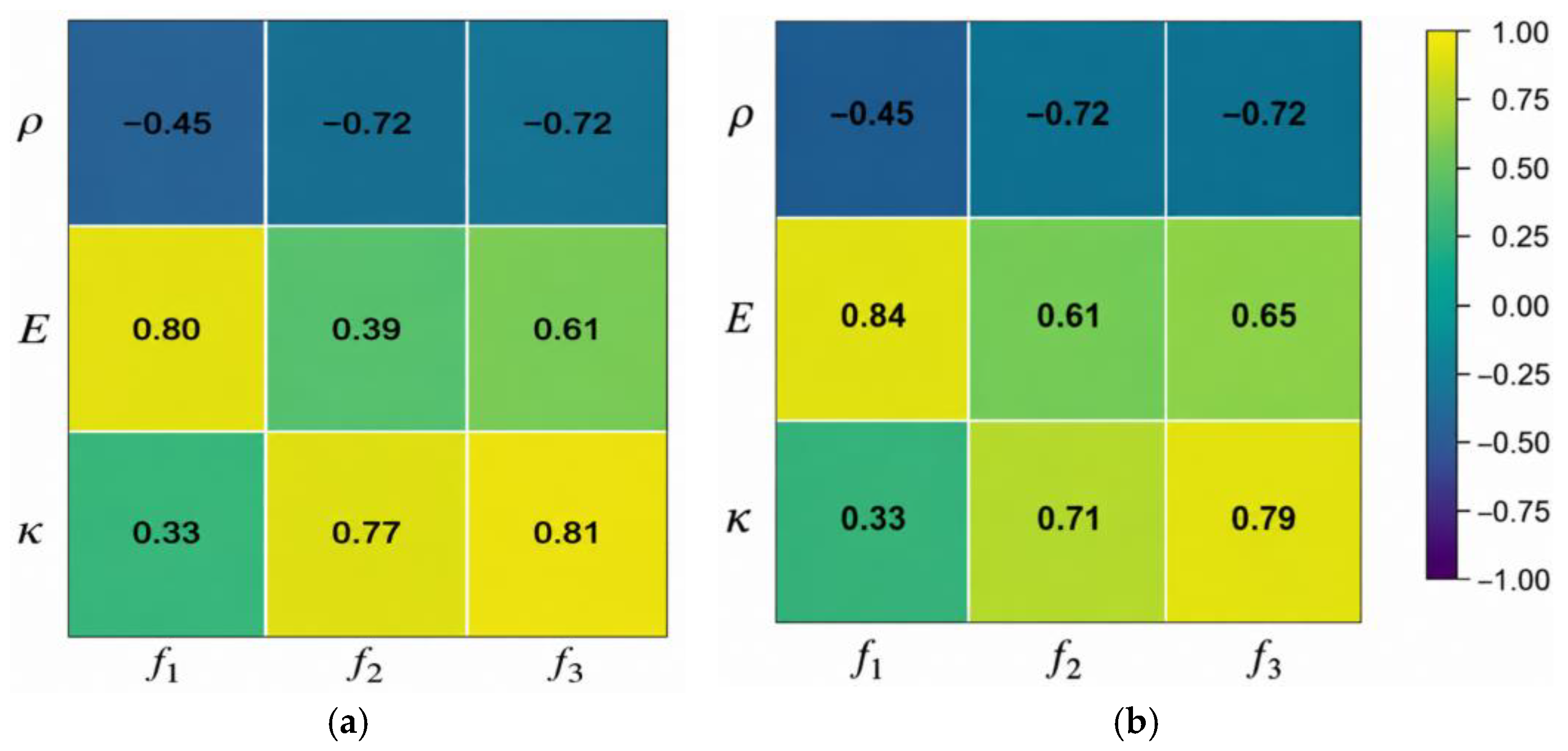
The differences between the Pearson and Spearman coefficients, particularly for E-f2 and $\kappa$-f2, indicate that the parameter–frequency relationships contained nonlinear but predominantly monotonic components. This supported the use of third-order candidate functions together with prescribed monotonic response directions. All three modal surrogates selected $\eta = 1$ through cross-validation, indicating Lasso-dominated sparse selection for the present dataset and candidate basis.

The monotonicity constraints were introduced to prevent non-physical local reversals rather than to improve the global prediction-error metrics. The prescribed negative density trend and positive modulus/support-stiffness trends were checked at both the modelling samples and 80 additional control points. The constrained surrogates retained independent-test R² values of 0.9988, 0.9496, and 0.9902 for the first three modes.

4.2. Weak Identifiability and Implications for FE Model Updating

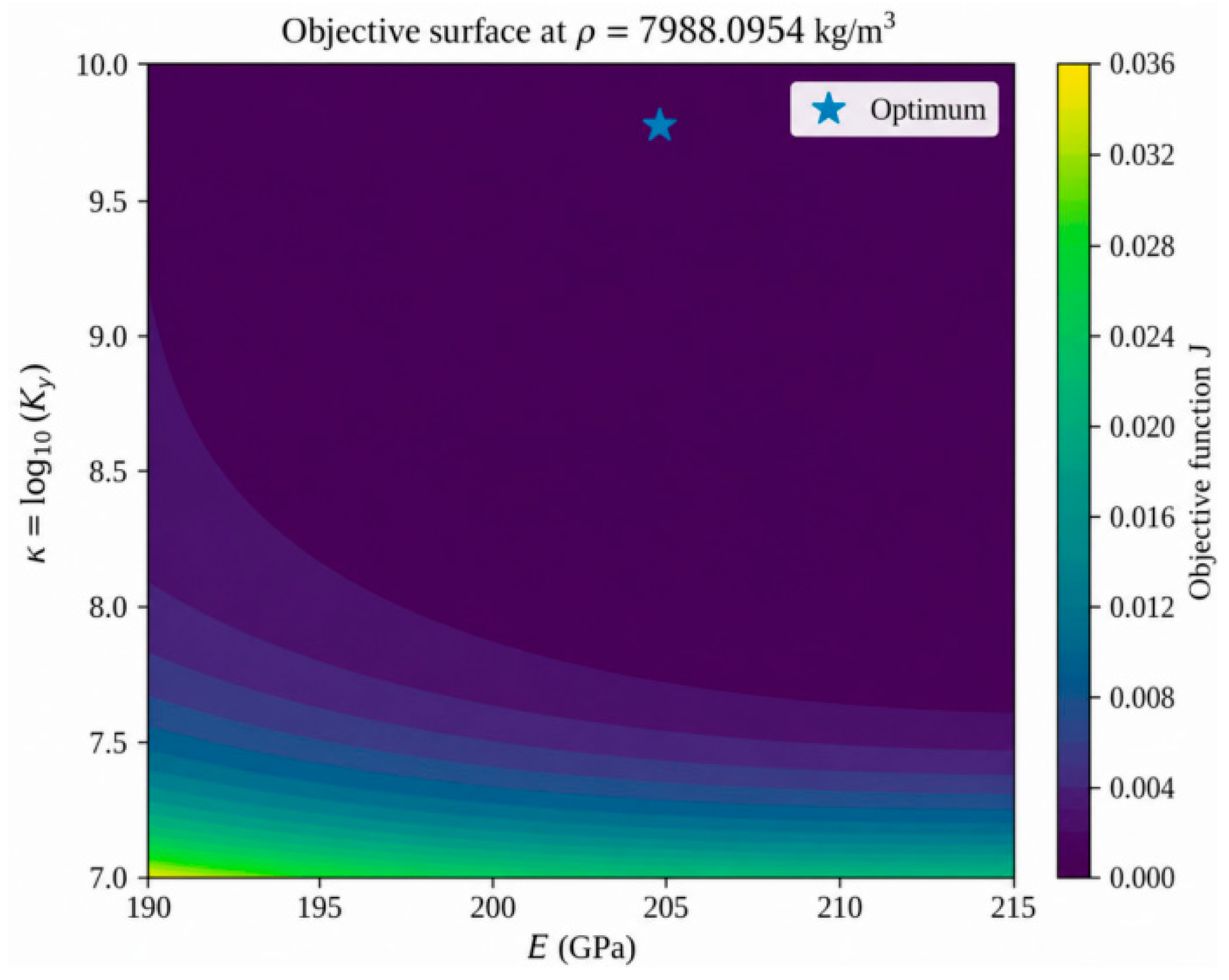
Near the optimum, the sensitivities of the frequencies to density and elastic modulus had similar magnitudes and opposite signs, indicating that their effects could compensate within the measured frequency vector. The support-stiffness logarithm showed stronger global correlations with f2 and f3 than local sensitivities at the optimum, consistent with the high-stiffness region of the identified solution.

The updated density was also checked against the specimen construction. The truss contains approximately 1000 connection bolts together with gusset plates and other hardware that are not all represented explicitly in the beam model. Expressing this omitted connection mass as an equivalent distributed mass gives an effective density of approximately 7.97 × 10³ kg/m³, close to the identified 7988.10 kg/m³. Because the bolt count and plate geometry are approximate, this is an order-of-magnitude consistency check rather than an independent density measurement.

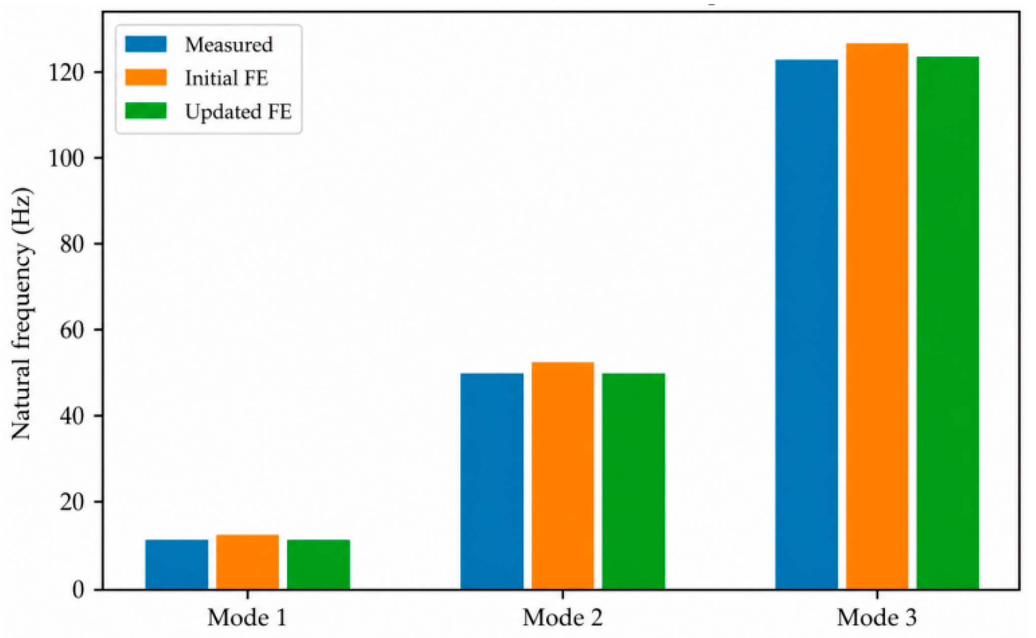
The elongated objective valley and the normalized Jacobian condition number of 112.17 indicate weak identifiability near the optimum. This is consistent with the wide bootstrap interval of Ky and its low local sensitivity in the identified high-stiffness region. The result limits the physical interpretation of the individual parameters but does not invalidate the response-level update: ANSYS back-substitution shows substantially better agreement with the measured modal frequencies.

The bootstrap estimates remained close to the optimum, but the unequal interval widths show that the three parameters are not identified with equal precision. The updated ρ, E, and Ky are therefore treated as a coupled calibration state constrained by the three measured frequencies rather than as independent measurements of material and boundary properties.

The bootstrap analysis quantifies modelling-sample and surrogate-refitting variability, whereas the Jacobian characterizes local identifiability. Experimental frequency-identification uncertainty was not separately propagated because repeated identification statistics were unavailable; this source of uncertainty can be incorporated when independent measurement-error information is available.

4.3. Methodological Implications and Comparison with Existing Approaches

Independent test-set validation and ANSYS back-substitution were used to distinguish surrogate accuracy from FE updating performance. The main computational cost lies in the generation of the high-fidelity FE database: one ANSYS modal analysis required approximately 62 s, corresponding to about 3.4 h for 200 serial evaluations. By comparison, sparse-surrogate fitting and the final inverse optimization each required less than 1 s.

The present application is low-dimensional, with three physically interpretable updating parameters. Elastic Net reduces the number of active polynomial terms but does not remove the rapid growth of the candidate space as parameter dimension increases. The framework is therefore most directly suited to low- and moderate-dimensional problems after dominant uncertain parameters have been identified. Higher-dimensional applications may require sensitivity screening, parameter grouping, active-subspace methods, or other dimension-reduction steps before surrogate construction.

5. Conclusions

A physics-constrained sparse response-surface framework was developed for finite element model updating using millimeter-wave-radar modal frequencies. The following conclusions were drawn:

(1)

Adaptive enrichment slightly increased the independent-test R² for all three modes, while cross-validation gating rejected unnecessary local corrections for the second and third modes.

(2)

The updated equivalent parameters were $\rho$ = 7988.0954 kg/m³, E = 204.8769 GPa, and Ky = 5.5889 × 10⁹ N/m. ANSYS back-substitution reduced the mean relative frequency error from 5.55% to 0.82%.

(3)

A Jacobian condition number of 112.17 and the broad bootstrap interval of Ky demonstrated stiffness compensation and weak identifiability. The updated parameters should therefore be interpreted as an equivalent combination constrained by the three measured frequencies, rather than as unique direct measurements.