Article

Explainable Ensemble Machine Learning Models for Bond Strength Prediction at Ultra-High-Performance-to-Normal-Strength-Concrete Interfaces


1
Nepal Research and Collaboration Center, New Baneshwor, Kathmandu 44600, Nepal
2
Department of Computer Science, University of South Dakota, Vermillion, SD 57069, USA
3
Department of Civil Engineering, Kantipur Engineering College, Tribhuvan University, Dhapakhel, Lalitpur 44700, Nepal
4
Department of Civil Engineering, Cosmos College of Management and Technology, Pokhara University, Lalitpur 44700, Nepal
5
Department of Civil Engineering, Lumbini Engineering Management and Science College, Pokhara University, Bhalwari 32903, Nepal
6
Department of Civil Engineering, Thapathali Campus, IOE, Tribhuvan University, Kathmandu 44600, Nepal
7
Department of Civil Engineering, Tribhuvan University, Kathmandu 44600, Nepal
*
Author to whom correspondence should be addressed.
Buildings 2026, 16(15), 3081; https://doi.org/10.3390/buildings16153081
Submission received: 21 May 2026 / Revised: 29 July 2026 / Accepted: 30 July 2026 / Published: 3 August 2026

Abstract

The slant shear bond strength of the UHPC-NSC interface is a key parameter governing load transfer and structural reliability in composite concrete members. However, accurate prediction remains challenging because of strong nonlinear relationships among influencing parameters and the limited availability of experimental data. This study presents an optimized machine learning framework for reliable bond strength prediction by integrating Extra Trees Regressor (ETR) and CatBoost (CATB) with Grasshopper Optimization (GO) and Northern Goshawk Optimization (NG) for hyperparameter optimization. Model performance was evaluated using cross-validation and independent testing to ensure reliable generalization. Among the developed models, the optimized CATB-NG achieved the highest predictive accuracy with an R2 of 0.934, RMSE of 3.081 MPa, and MAE of 2.186 MPa. SHapley Additive exPlanations (SHAP) identified NSC surface treatment and compressive strength as the dominant factors influencing bond strength, while Individual Conditional Expectation (ICE) analysis revealed nonlinear feature interactions and threshold behaviors. To facilitate practical engineering applications, the optimized model was implemented in a graphical user interface (GUI) for real-time prediction with standardized feature encoding. The proposed framework provides an accurate, interpretable, and user-friendly tool for predicting UHPC-NSC interfacial bond strength and supports engineering design and decision making.

1. Introduction

With the aging of infrastructure due to harsh environmental effects (such as freeze–thaw cycles, chloride ion attack, and sustained loading), the need for effective rehabilitation measures for existing reinforced concrete structures has increased continuously [1,2]. Here, conventional repair materials do not offer good mechanical compatibility and durability, and often exhibit premature failure between old and new concrete. Adequate bonding between the existing substrate and the overlay is required to achieve sufficient strength in repaired or strengthened members for resistance against long-term loads and safety [3]. Poor bonding can cause delamination, cracking, or even complete detachment of the repair layer, leading to a considerable decrease in the useful life of the structure [4].
In recent years, UHPC has received considerable attention as an excellent repair and strengthening material that possesses superior mechanical, durability, and rheological properties when compared to NSC [5,6]. UHPC attains a compressive strength higher than 120–150 MPa, flexural strength of approximately 50 MPa, and direct tensile strength greater than 5 MPa [7,8]. These unique properties are attributed to its high particle packing density, optimized water-to-binder ratio (typically less than 0.2), and content of fine supplementary cementitious materials, such as silica fume and slag [9]. Several factors, such as surface preparation, interface moisture state, curing environment, sequence of casting, degree of surface roughness, content of reinforcing fibers, and compressive strength of substrate, affect bond strength [10,11]. Among them, surface texture and roughness have been well-accepted as being critical parameters influencing bond strength [12,13]. Higher friction and interlocking are achieved between the UHPC overlay and NSC substrate due to the rough surfaces. Studies by Tayeh et al. [14] found that slant shear bond strength for sandblasted and grooved surfaces increased by 105% and 60%, respectively, over smooth surfaces. Farouk et al. [15] found that deeper grooves and higher substrate compressive strength contributed to better resistance in UHPC–NSC columns. Similarly, Horak et al. [16] stressed that the protrusions of interfaces were crucial to activating the shear strength. Santos et al. [17] also demonstrated that improved roughness and surface cleanliness can play a large role in increasing (mechanical) adhesion, although the influence of moisture content can modulate this effect.
The bond formation mechanism is relatively sensitive to the moisture condition at the interface [18]. Zhang et al. [19] observed that composites cured at normal temperature showed a better interfacial quality than those cured under pressure or steam. At moderate curing, hydration reactions induce a denser microstructure in the ITZ. Their findings show that the tensile bond strengths between UHPC and NSC were 90 to 142% of those for NSCs. Microstructural studies by Haber et al. [20] and Feng et al. [21] have demonstrated that UHPC–NSC interfaces typically exhibit lower total porosity and more developed C–S–H, resulting in improved mechanical interlocking and chemical adhesion. To assess the mechanical behavior of the UHPC–NSC interface, different testing techniques have been used, such as slant shear, splitting tensile, pull-off, and direct shear tests [22,23]. Of these, the slant shear test has become the most popular and dependable method for measuring interfacial bond strength under combined stress conditions. Lessly et al. [24] observed that the curing process also played a vital role in the strength gain of UHPC concrete, where steam curing was found to be superior to other normal and heat curing techniques.
Khaksefidi et al. [25] investigated the bond of UHPC to high-strength steel bars and to ordinary strength rebar. Nevertheless, an increase in the rebar diameter resulted in a slight decrease in the maximum bond stress. It is interesting to note that the effect of bond length on the maximum bond stress was opposite in both materials: increasing bond length enhanced the maximum bond stress in NSC, while it had a detrimental effect on UHPC. Likewise, Huang et al. [26] investigated the microstructure of ITZ between lightweight concrete (LWC) and NSC. Due to the porous character of LWC, they noted that surface roughness is important for developing a good bond between two concretes. A large part of previous studies has been based on empirical or semi-empirical methods to determine the BS. While these models accurately describe the data upon which they were developed, their predictive precision of prediction frequently diminishes when extrapolated to new data [27,28].
To overcome the deficiency of the empirical formula, ML methods have been applied to predict bond strength with better reliability in recent literature. Several studies across different domains have used advanced ML modeling and explainable artificial intelligence for civil engineering prediction problems [29,30,31,32,33,34,35]. These algorithms have been shown to perform better in the predictive sense than classical equations, but they might not completely capture complex nonlinear behavior. Feng Zhang et al. [36] used classical and modern ML techniques to predict the interfacial bond strength for FRP-concrete and reported 50% less prediction error from their XGBoost model compared to that of empirical models. Su et al. [37] adopted several MLR, SVR, and ANN models to estimate the bond strength between FRP and normal concrete. They achieved values amounting to their determination’s coefficient being 0.85. Hiew et al. [38] developed and applied a hybrid deep learning neural network methodology to predict the stress–strain behavior of confined UHPC subjected to different loadings and environments. Farouk and Jinsong [39] developed a quantitative ML-based method to estimate the interfacial bond strength between UHPC and NSC from experimental bond data. Their study demonstrated that the prediction accuracy of nonlinear models was better than that of classical empirical equations, which indicates the ability of data-driven approaches to reflect complex UHPC-NSC bond behaviors. Likewise, using 113 experimental samples, Lazaridis and Thomoglou [40] presented an explainable model-ensemble machine learning framework for predicting the shear capacity of TRM-strengthened masonry walls. An optimized voting classifier of XGBoost and CatBoost (for R2, 0.95; for MAPE, 8.03%) with SHAP analysis and web application improved interpretability and practical applicability of the model. Gray et al. [41] proposed an explainable machine learning framework for the prediction of shear capacity of modular cold-formed steel beams using 105 validated finite element models. CatBoost yielded the highest accuracy (R2 = 95.9% and MAPE = 6.49%), while SHAP analysis identified the top influencing variables, and empirical 95% prediction intervals improved prediction reliability. Sapkota et al. [42] adopted ensemble ML for the prediction of interfacial bond strength of UHPC-NSC using split tensile and slant shear test data. Their findings showed that gradient boosting and CATB achieved a high accuracy of an R2 up to 0.96, highlighting the significance of surface treatment as an influential factor. Likewise, Liu et al. [43] developed a quantitative ML model to predict the UHPC-NSC interfacial bond strength based on 95 slant shear test specimens. Their CATB model provided excellent predictions, with an R2 of 0.948, RMSE (root mean square error) of 1.408, and MAE (mean absolute error) of 1.028, which respectively surpassed those obtained by neural networks, ensemble models, and empirical design equations. The research also quantified surface treatment, joint angle, and NSC-CS as the most significant parameters controlling the bond behavior at the interface.
Tian et al. [44] used ML for prediction the interfacial bond strength of FRP bars on 158 pull-out tests. Among 12 algorithms trained, CatBoost provided the best accuracy (an RMSE 58.3% lower than that of the existing analytical equation proposed by Tian et al., which was statistically best-performing), and feature importance using a light gradient boosting model revealed rib width to be the primary parameter influencing bond performance. Li et al. [45] suggested a new framework for predictive modeling of the interface bond strength between UHPC and NC based on surface damage parameters using XGBoost. The model was highly predictive, achieving R2 values of 0.95 and 0.94 for the training and testing datasets, respectively. Ecemis et al. [46] used experimental tests and a hybrid PINN-CatBoost model on the sustainable concrete with waste tire rubber and recycled steel fibers. The optimized mixture achieved a 6% greater compressive strength compared to control mixtures, and the hybrid framework successfully predicted strength with the expository ability of combining physics-informed learning techniques with explainable artificial intelligence.
Singh et al. [47] presented a ML framework developed to predict the normalized bond strength of reinforced concrete after exposure at high temperatures using 458 experimental data. The top predictive performance of XGBoost had an R2 testing value of 0.9417 out of twelve regression algorithms, and the feature importance analysis identified that exposure temperature and bond degradation were the salient governing parameters.
Taffese et al. [48] conducted a study based on a database of 170 samples in which the model established an XGBoost ensemble for the ultimate moment capacity prediction of UHPC-strengthened reinforced concrete members. The optimized model made predictions with an R2 of 92.5% (training) and 81.9% (testing), exhibiting relative superiority for tree-based ensemble models, while also identifying reinforcement ratio, the thickness of UHPC, and height of member as the most impactful design parameters. In one study by Mehdizadeh et al. [49], a Bayesian-optimized ML framework was proposed for predicting bond strength in externally bonded reinforcement on groove (EBROG) systems. Out of four models, XGBoost was the most accurate model in predicting value with an R2 = 0.987 and RMSE = 0.522 kN. SHAP analysis finally identified fracture energy as the factor that greatly influences control variables which affect bond strength.
Zhan et al. [50] carried out an ML approach to predict the mechanical and interfacial properties of concrete materials from experimental data. They found that ML models were able to accurately predict the datasets that had an R2 over 0.90 and remarkably lower error than those provided by common regression methods. The analysis showed the superiority of data-driven models in performing nonlinear relations between material properties and performance.
Several studies on explainable AI have been reported that capture insights on the details of concrete using advanced modeling. For instance, Katlav and Turk et al. [51] proposed an explainable stacked machine learning framework for predicting the bond strength retention of FRP bar-concrete systems in marine environments using 601 experimental samples. The optimized XGB-LGBM stacked model produced the highest testing performance (R2 = 0.845 and R = 0.935), whilst SHAP and ICE analyses uncover concrete compressive strength, conditioning duration, and conditioning temperature as the main contributors to long-term bond durability.
By using a database of 146 samples and 16 input variables, Abid et al. [52] developed four machine learning models to predict the interlayer bond strength of 3D-printed concrete. XGBoost achieved the best predictive performance with training and testing R2 values of 0.999 and 0.998, respectively, while printing speed, superplasticizer/binder ratio, water/binder ratio, thixotropic agent, and time interval were identified as the main influencing factors by SHAP, ICE, and PDP analysis.
Zhang et al. [53] developed an explainable GA-optimized machine learning framework to predict the bond strength between steel-FRP composite bars and concrete using 241 pull-out specimens. The GA-SVR model achieved superior predictive accuracy with a testing R2 of 0.963, outperforming existing empirical equations, while SHAP and 3D-PDP analyses confirmed the underlying bond mechanisms and supported the development of a practical GUI for engineering applications.
Al-Hamd et al. [54] developed seven machine learning models to predict the bond strength of reinforced and fiber-reinforced concrete under ambient and elevated temperatures using 394 experimental samples. Gradient Boosting, XGBoost, and Decision Tree achieved the highest predictive performance with testing R2 values exceeding 0.95, while SHAP analysis identified the length-to-diameter ratio and failure surface temperature as the dominant variables governing bond behavior. Kashani et al. [55] proposed a multi-output explainable machine learning framework to predict ultimate and relative bond strengths of corroded reinforcing bars. XGBoost also showed a stronger predictive ability with R2 = 0·977 for ultimate bond strength and R2 = 0·966 for relative bond strength, while SHAP analysis indicated that variables most responsible were corrosion level, compressive strength and yield strength.
Likewise, Khorshidi et al. [56] adopted an explainable multi-objective AI framework for sustainable fly ash concrete design using a database of 1,062 concrete mixtures. NGBoost demonstrated the best predictive performance (R2 = 0.92, RMSE = 4.897 and MAE = 3.492), while uncertainty analysis and nature-inspired multi-objective optimization enabled the generation of Pareto-optimal concrete mixtures with enhanced strength and reduced CO2 emissions.
Nikzad et al. [57] developed an explainable transformer-based AI framework for simultaneous prediction of concrete fracture energy and fracture toughness using 330 experimental samples. Among 25 machine learning algorithms, TabPFN achieved the highest testing accuracy (R2 = 87.89%), while SHAP analysis revealed that tensile strength, beam depth, and notch geometry predominantly governed the fracture properties through nonlinear interactions.

2. Research Significance

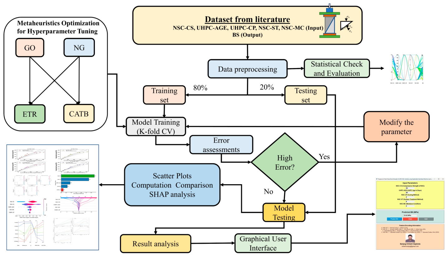
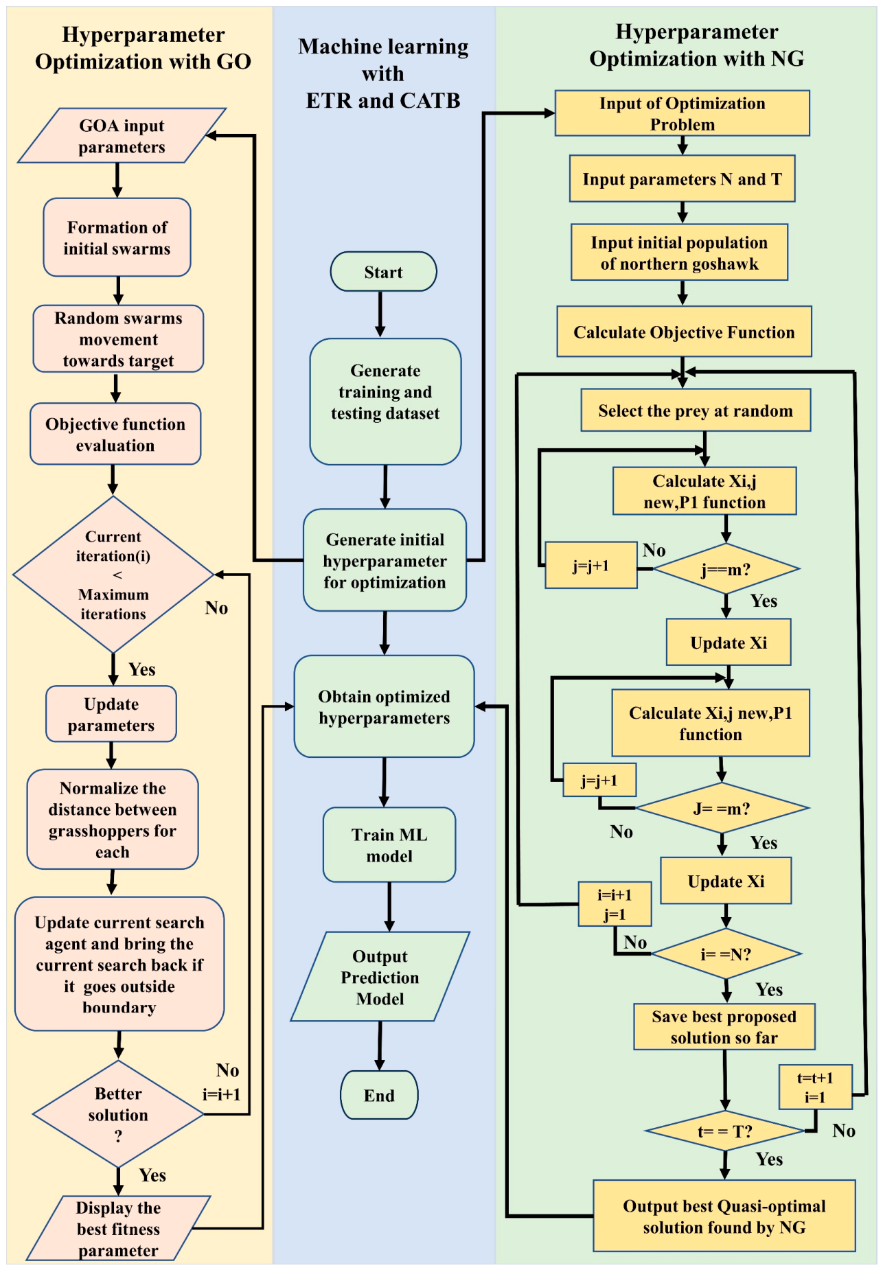
The performance of the bond between UHPC and NSC at their interface must be reliably predicted for the design and rehabilitation of composite structures. The slant shear bond strength (SSBS) test is an essential parameter for indicating the interfacial quality, and its performance prediction is still problematic due to the nonlinear interaction of parameters, including surface roughness, heat curing regime, fiber volume fraction CS, and water-to-binder ratio. Classical empirical or regression-based models assume a large simplification of such interdependencies, often leading to spatially and case-specific predictions. Although ML approaches have been developed for modeling concrete in the past, many previous studies suffer from poor hyperparameter tuning and training, local convergence, or a lack of explanation/interpretation, resulting in numerically accurate but unreliable models. As such, a framework that can be used to improve predictive capability and, further, provide insight into the impact of controlling parameters on bond strength is essential in the field of contemporary materials science. The workflow diagram of the current study’s process is presented in Figure 1. The novelties of the current study are:
  • A novel hybrid machine learning framework integrating Extra Trees Regressor and CatBoost with Grasshopper Optimization (GO) and Northern Goshawk Optimization (NG) is proposed to improve the prediction accuracy and generalization capability of UHPC-NSC slant shear bond strength through intelligent hyperparameter optimization. Such optimizers enhance model robustness by efficiently tuning hyperparameters while mitigating premature convergence to local optima, a common limitation of metaheuristic search algorithms. By maintaining an effective balance between global exploration and local exploitation, the optimization process is more likely to identify near-optimal hyperparameter configurations, thereby improving predictive accuracy and generalization performance on unseen datasets.
  • A comprehensive comparative investigation is conducted by jointly evaluating predictive accuracy, computational efficiency, and optimization performance, providing a balanced assessment of the trade-off between model robustness and computational cost for practical engineering applications.
  • An explainable artificial intelligence framework is established by combining SHAP and Individual Conditional Expectation (ICE) analyses to quantify both the global importance and local nonlinear influence of key material, curing, and interface parameters governing slant shear bond strength.
  • A user-oriented graphical user interface (GUI) is developed to translate the optimized machine learning models into a practical engineering decision-support tool, enabling rapid bond strength prediction and interactive visualization without requiring programming expertise.
  • An integrated prediction and interpretation framework is presented that combines metaheuristic optimization, ensemble learning, explainable artificial intelligence, and GUI-based deployment within a single workflow, providing an accurate, transparent, and practically applicable tool for UHPC-NSC interfacial bond strength assessment.
Figure 1. Workflow diagram of the proposed modeling process.
Buildings 16 03081 g001

3. Methodology

3.1. Data Collection

The quality, diversity, and structure of the dataset for model training and validation are the basis for any machine learning method’s performance. In the present study, an advanced database was used for predicting the interfacial bond strength between UHPC and NSC. These datasets are composed of 133 experimental data points taken from the literature and used for the bond test used by Farouk and Jinsong [39] and Sapkota et al. [42]. The dataset was pre-processed and labelled for distinction between input parameters and target output to reduce noise and enhance model interpretability. The input variables are as follows: UHPC-Age, NSC-CS, NSC-CP, the surface treatment of the NSC (NSC-ST), and its moisture condition (NSC-MO). The NSC surface treatment is a multilevel independent variable, grouped into 6 categories: smooth (SM), wire brushed (WB), drilled holes (DH), sandblasted (SB), rough surface (RS), and grooved surface (GS). The curing system is denoted as 1 for natural curing and 2 for steam curing, while the condition of moisture exposure is generalized as 1 (surface dry-saturated), 2 (air-dry surface), 3 (surface wet-saturated). This encoding scheme (which is structured) results in a way of encoding categorical variables so that they can be well understood by ensemble learners and optimization algorithms. A unified encoding strategy was adopted throughout the study to ensure identical preprocessing across all hybrid models and enable a consistent comparative evaluation of the proposed optimization frameworks. Given that the developed models are based on tree ensemble learning, which partitions the feature space using decision rules rather than distance metrics, the categorical encoding serves only as an identifier for category membership. Although the compiled database consists of 133 experimental observations, such dataset sizes are common in machine learning applications within structural and concrete engineering because experimental testing is costly and labor-intensive. It should be emphasized that the proposed study does not require separate datasets for each hybrid model. Instead, the same database was consistently used to develop and comparatively evaluate four alternative optimized machine learning frameworks under identical validation protocols. Moreover, Extra Trees Regressor and CatBoost are tree-based ensemble algorithms that have demonstrated robust performance on structured datasets of limited size, while the applied metaheuristic optimization algorithms only optimize model hyperparameters without increasing the number of trainable parameters. Therefore, the adopted modeling framework is considered appropriate for the available experimental database. The dataset supplies a well-balanced and physically meaningful description of the interfacial parameters influencing bond strength, thus forming a reliable platform for resilient predictive modeling.

3.2. Data Preprocessing and Analysis

The features of the dataset are six in number, where there are input and output variables, regarding the statistically important parameters such as mean, median, standard deviation, minimum, maximum, and a record of the range. The data preprocessing and numerical computations were performed using the Pandas and NumPy libraries implemented in Python Programming V3.14 [58,59,60].
The statistical details of all the input features are tabulated in Table 1. NSC-CS has a mean of 47.16 MPa and a median value of 45 MPa among the input features, showing a slight skew of the distribution. The standard deviation of 5.16 indicates moderate dispersion around the mean, resulting in minimum and maximum values of 31.9 MPa and 57.4 MPa, respectively, providing a range width of 25.5 MPa. Likewise, UHPC-AGE exhibits a large dispersion (the mean is 22.8 days for a standard deviation of 25.43, which spans between a minimum of 2 and a maximum of 180 days (range 178 days), highlighting significant variations in the duration of curing. The categorical variable UHPC-CP ranges from 1 to 2 (mean = 1.56, standard deviation = 0.49), indicating that the curing process is likely a binary classifier.
The second input feature is NSC-ST with an average value equal to 4.74 and a median equal to 6, indicating a nonhomogeneous distribution. The 2.07 standard deviation indicates moderate variance across data points. Similarly, NSC-MC has a mean of 1.72 and a median of 2, with a lower standard deviation of 0.55, indicating relatively similar values of moisture content in the database, with values limited between 1 and 3 (range width: 2). The only output feature, BS (bond strength), has a mean of 16.03 MPa and a median of 14.69 MPa, and it shows some skewedness. Due to a high standard deviation of 9.04 MPa, the bond strength values spread widely in range, a minimum of 1.19 MPa and a maximum of 41.2 MPa, for a total of 40.01 MPa. This may imply a wide range of bond strengths, not least due to the range of input conditions in the training set.
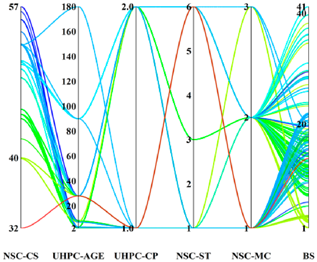
Figure 2 shows a visualization of the relationships between the six features -NSC-CS, UHPC, UHPC-CP, NSC-ST, NSC-MC, and BS through a parallel coordinate graph. Having one line for each data instance, the color differences in each line reflect different response patterns. NSC-CS values range from 32 MPa to 57 MPa, with significant dispersion. The values of UHPC-AGE range from 2 days to 180 days. These longer concrete ages might affect the values of higher bond strength. The UHPC-CP variable is categorical with values that range between 1 and 2. Also, NSC-ST varies from 1 to 6, which visually represents different material treatments. Similarly, depending on moisture conditions, NSC-MC values range between 1 and 3. There seems to be a heavy clustering near lower bond strength values, when the output variable BS varies from 1.19 MPa to 41.2 MPa. An inverse relationship seems to arise from trends between UHPC-AGE and BS, where lower values of age correspond to a lower bond strength. Similarly, the relationships between NSC-ST and NSC-MC also show various correlation patterns in which specific moisture content, surface fugacity, or treatment may improve bonding performance. Overall, this visualization indicates potential nonlinear relationships, which would require more complex statistical or machine learning approaches to generate meaningful insights into which parameters are impacting BS.

3.3. Machine Learning Models and Optimization Techniques

3.3.1. Extra Tree Regressor

Extra Trees Regressor (ETR) is a tree-based ensemble learner. It builds many unpruned decision trees and averages their predictions [61]. Technically, ETR differs from Random Forest Regressor in the way randomness is incorporated during tree construction. While Random Forest is based on bagged samples and searches for the best split among the randomly selected features, ETR applies all the training data in each tree and chooses to pick up thresholds from different random values to obtain a new root candidate feature. The best split is selected amongst those generated thresholds, using a criterion of variance reduction. This frees us from the burden of searching for the best split points and simplifies the tree-growing procedure. The aggressive randomization scheme of ETR results in strong variance reduction over the ensemble, leading to an improved generalization performance [62]. But such randomness leads to model bias since some useful cut points, or weakly influential features, might be ignored. Nevertheless, the bigger trade-off in our senses is inevitable, and yet across all examples, ETR trains faster than Random Forest, and it induces less overfitting. Technically, ETR is especially efficient to model highly nonlinear systems with complex feature interactions, as increasing diversity among trees improves robustness and stability of predictions while being computationally cost-effective.

3.3.2. Catboost Regressor (CATB)

CatBoost Regressor (CATB) is an ensemble model based on gradient boosting, which builds an additive function consisting of many weak learners, namely symmetric decision trees, also called oblivious trees [63]. In this arrangement, every tree applies the same splitting function and threshold at each level, leading to a balanced and regular tree structure. This model leads to lower variance and better generalization properties as compared to the conventional decision tree; it also improves upon the stability of a learning process by combining it with a strong learner that reacts to less important features (especially for tabular data with mixed feature scales and compositional or nonlinear interactions), like concrete mix composition and age. CatB trains the models one-by-one: each new tree is trained to eliminate the error of the current ensemble by means of gradient optimization with a prescribed loss function (usually mean squared error when considering regression). A crucial technical strength of CatB is its ordered boosting, which prevents target leakage in training via the constraints on the predictions for each sample that are made with the models fitted on earlier samples according to a prespecified order [64]. This method considerably decreases the influence of overfitting for small to moderate datasets that are encountered in civil engineering practice. CatB implicitly grasps high-order feature interactions without relying on hand-crafted feature engineering, and it supports precise, consistent feature attribution out-of-the-box with its native SHAP value support for tree ensembles. Consequently, CatB is a powerful high-capacity nonlinear regressor capable of accurately approximating complex input–output mappings combined with strong generalization capability and interpretability.

3.3.3. Grasshopper Optimization (GO)

The life cycle of a grasshopper can be divided into three stages: egg, nymph, and adult. Both nymphs and adults show swarm behavior [65]. In the larval phase, the grasshoppers jump and move like rolling cylinders. The swarm in this stage moves slowly, and the steps are small. In the adult phase, grasshoppers form a swarm in the air. The swarm in this stage moves abruptly and in large steps. Grasshoppers also display food source and target seeking.
The mathematical model to simulate the swarming behavior of grasshoppers is as follows:
X i = r 1 S i + r 2 G i + r 3 A i
Here, X i = position of ith grasshopper; S i = social interaction; G i = gravity force on the ith grasshopper; A i = wind advection; r 1 , r 2 , r 3 = random numbers between 0 and 1.
S i = j = 1 , j i N S d i j · d ^ i j d i j = | x j x i | S r = f   e r l e r d ^ i j = x j x i d i j f = 1.5 l = 0.5
Here, d i j = distance between ith and jth grasshoppers mapped in the interval [1,4]; S(r) = function to define strength of social forces; d ^ i j = unit vector from ith to jth grasshoppers; f = intensity of attraction; l = attractive length scale; N = number of grasshoppers.
G i = g e ^ g
Here, g = gravitational constant, e ^ g = unit vector towards the center of the Earth.
A i = u e ^ w
Here, u = constant drift, e ^ w = unit vector in the direction of wind. Substituting the values of S i , G i , and A i in Equation (1), we get:
X i d = j = 1 N S | x j x i | x j x i d i j g e ^ g + u e ^ w
The above equation is modified so that the model converges to a specific point.
X i d = C j = 1 , j i N C u b d l b d 2 S | x j d x i d | x j x i d i j + T ^ d C = c m a x l c m a x c m i n L
Here, cmax = maximum value = 1; cmin = minimum value = 0.00001; l = current iteration; L = maximum iteration; C = decreasing coefficient to shrink the comfort zone, attraction zone, and repulsion zone; u b d = upper bound in the dth dimension; l b d = lower bound in the dth dimension; T ^ d = value of the dth dimension in the target (best solution found).

3.3.4. Northern Goshawk Optimization (NG)

The northern goshawk, a medium-large hunter in the family Accipitridae with an intelligent process in hunting and catching prey, is used for a mathematical model. Its hunting technique is divided into two stages. Firstly, it identifies the prey and moves towards it at a high speed, and secondly, it hunts the prey in a short-tail chase process [66]. The main inspiration in designing the proposed NGO algorithm is its mathematical modeling of the mentioned strategy.
x 1,1 x 1 , d x 1 , m y x i , 1 x i , d x i , m y x N , 1 x N , d x N , m N × m ,
The matrix X represents the population of northern goshawks, where Xi denotes the ith proposed solution. Each element xi,j corresponds to the value of the jth variable in the ith solution. The matrix has the dimensions N × m with N being the number of population members and m being the number of problem variables.
F ( X ) = F 1 = F X 1 F i = F X i F N = F X N N × 1
The vector F represents the objective function values for the northern goshawk population, where Fi is the objective function value for the ith proposed solution.
P i = X k , i = 1,2 , , N , k = 1,2 , , i 1 , i + 1 , , N , x i , j n e w   , P 1 = x i , j + r p i , j I x i , j , F P i < F i , x i , j + r x i , j p i , j , F P i F i ,                                           X i = X i n e w , P 1   , F i n e w , P 1   < F i , X i , F i n e w , P 1   F i ,                                                                                        
where k is a random natural number in the interval [1, N], Pi is the location of the prey for the ith northern goshawk, and Fp is the value of its objective function. r is a random number in the interval [0, 1], I is a random number that can be 1 or 2, xi new P1 is the new status for the ith suggested solution, xi,j new P1 is its jth dimension, and Fi new P1 is its objective function value based on the first phase of NGO.
X i , j new   , P 2 = X i , j + R 2 r 1 X i , j , R = 0.02 1 t T , X i = X i new   , P 2 , F i new   , P 2 < F i , X i , F i new   , P 2 F i .
where T is the maximum number of iterations and t is the iteration counter. Fi nex P2 is its objective function, xi new P2 is the new status for the ith suggested solution, and xi,j new P2 is its jth dimension value based on the NGO’s second phase.

4. Model Development and Performance Metrics

The base ensemble learners in this work were ETR and CATB. Extra Trees Regressor was implemented using the Scikit-learn machine learning library [67], whereas the CatBoost model was developed using the CatBoost framework [68]. The predictive ability of these machine learning techniques was improved when tied to GOA and NGOA metaheuristic optimization algorithms. This hybridization resulted in four final models, ETR–GO, ETR–NG, CATB–GO, and CATB–NG. The hybridization of ensemble and metaheuristics models is depicted in Figure 3.
The metaheuristic algorithms were utilized to optimize the main hyperparameters of the base models for better accuracy and stability. For computational efficiency and methodological coherence, a restricted optimization was performed using the top three most impactful hyperparameters for each base model: number of estimators, learning rate, maximum depth for CATB; and number of estimators, minimum samples split, and number of features for ETR. These parameters have the strongest effect on generalization and learning behavior of models without excessively widening the search space.
In the present study, the K-fold cross-validation method is used to validate the model and address the overfitting issues and bias estimation of the performance of predictive models [69]. In this k-divide approach, we partition the dataset into k-sets of approximately equal size and independently use one set for training and the remaining sets for validation. This is repeated k times until every data subset can be used for validation, and the model’s performance is averaged out among all folds. This sort of procedure is a much stronger and more unbiased estimate of model generalization than a single train–test split, greatly reducing the risk of overfitting and the associated scenario where one builds a model that works well on the training data but terribly on new data. For the current study, the dataset was first split into 80% for training and 20% for testing. The test split was strictly maintained and only used for final evaluation to give a fair performance estimate of the developed models.
The process of two-way-fold cross-validation was carried out to maintain computational efficiency and methodological stability. During the optimization process, each candidate solution generated by GO or NGO was validated using a 3-fold cross-validation on the training set. This initial verification allowed for the relative comparison of competitive configurations and reduced the calculation overhead required to perform optimization. When the metaheuristic algorithm converged towards an optimal architecture, a more comprehensive 5-fold cross-validation was then utilized for the tuned model to achieve a reliable estimation of its predictive performance. Finally, the model was retrained with tuned hyperparameters on the entire training set and tested against an unseen 20% test set to determine its ability to generalize.
For ETR-GO and ETR-NG, the min_samples_split (with a value between 1 and 10) is the minimum number of samples required to split an internal node; as its value decreases, it results in finer splits and thus higher complexity. Ideally, ETR-GO has three; ETR-NG has two, revealing somewhat more aggressive splitting in the GO-optimized model. The max_depth controls the depth of the decision trees between 1 and 10, which avoids extreme overfitting. The best depths are seven (ETR-GO) and seven (ETR-NG), meaning deeper trees perform better, but it gets trickier to balance. The n_estimators (ranging from 10 to 100) corresponds to the number of trees in the ensemble, which affects the accuracy and also the time needed to compute the model. The maximum value of ETR-GO is 85, and for ETR-NG, it reaches 66, which indicates the genetic-optimized model requires a higher number of estimators than the other models. Likewise, the learning_rate ranges from 0.1 to 1), in addition to the hyperparameters mentioned above. Smaller values cause slower but more stable learning that mitigates divergence. In GO, CATB-GO yields and selects 0.17 optimally, and 0.11 in CATB-NG, indicating a faster learning rate imposed on GO. We can observe that max_depth (1 to 10) follows the same pattern as in ETR, with three vs. six for CATB-GO and CATB-NG, with the GO-optimized model favoring more shallow trees. For CATB-GO, n_estimators (10 to 100) is found to be 97, while CATB-NG converges on 89, suggesting the GO preference for more trees. The metaheuristic algorithm (MHA) parameters of n_pop = 20, max_iter = 100, and dim = 3 suggest that this optimization was performed with a population size of 20, 100 iterations, and three as the search dimension, ensuring good exploration of the hyperparameter space. All the details of hyperparameters are presented in Table 2.
Hyperparameter tuning plays a vital role in optimizing the base algorithm and its associated performance [70,71]. The performance of the base and optimized models is distinguished based on the statistical indices. The metrics help to validate the model for generalizability and prediction ability. The statistical metrics used in the study are Coefficient of Determination (R2), Root Mean Squared Error (RMSE), Mean Absolute Error (MAE), Willmott’s Index of Agreement (WI), and Ratio of the Root Mean Square Error to the Standard Deviation Ratio (RSR), and are presented in Equations (11)–(15).
R 2 = i = 1 n ( Y i Y m ¯ ) 2 i = 1 n ( Y i Y i ) 2 i = 1 n ( Y i Y m ¯ ) 2
RMSE = 1 n i = 1 n ( Y i Y i ) 2 2
MAE = 1 n i = 1 n ( Y i Y i )
WI = 1 i = 1 n ( Y i Y i ) 2 i = 1 n Y i Y m ¯ + Y i Y m ¯ 2
RSR = R M S E 1 n i = 1 n ( Y i Y m ¯ ) 2 2
Y i is the actual ith value, Y i is the predicted ith value, n is number of data samples in a dataset, and Y m ¯ is the mean of actual values.

5. Results and Discussion

5.1. Comparison of Predictions of Different ML Models

The quantitative performances of four hybrid models with ensemble tree regressors and two optimization strategies are listed in Table 3. All graphical representations were generated using the Matplotlib V3.11 visualization library [72]. The explained variance was quantified by the parameter R2. Values near one imply more powerful predictability. On the training set, CATB NG has a maximum R2 = 0.999, and CATB-GO yields an R2 of 0.996. This indicates near-perfect fitting. Certainly, error-based metrics concur with this trend. RMSE and MAE are used to measure the absolute and average differences between predicted and observed bond strengths. The CATB-NG has the lowest RMSE value of 0.2183 MPa and MAE value of 0.164 MPa, indicating little residual error. The WI tests the match between prediction and measurements. The values tend to unity for all models and are approximately one for the CATB-based ones. RSR (RMSE/standard deviation of observations) is used to assess model performance. Lower values indicate better performance. The best-performing CATB-NG is once again the one with an RSR of 0.025. In the testing set, performance tends to degrade as expected, but the position is maintained with consistency. CATB-NG still has the best generalization ability with an R2 of 0.934 and the smallest RMSE of 3.081 MPa.
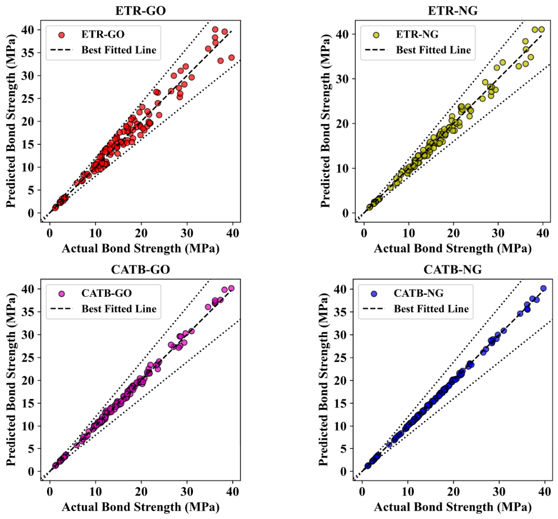
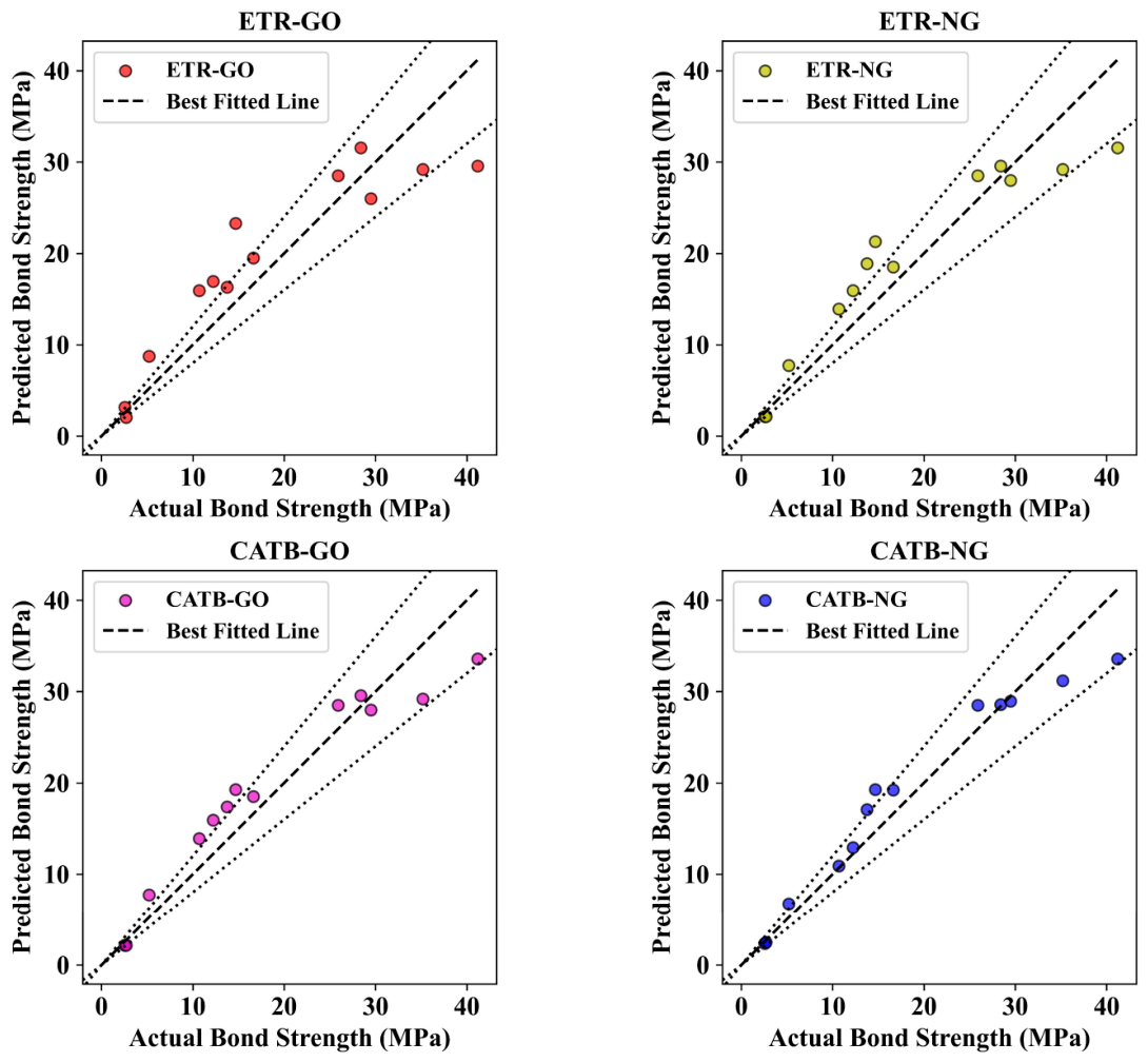
In Figure 4, the actual bond strength is plotted against the predicted one for the training data. Each subfigure is associated with one model. The black diagonal reference line indicates a perfect one-to-one relationship between predicted and measured values. The dashed line represents the best linear regression fit according to the model prediction. The two dashed lines indicate the acceptable deviation strip around the ideal rule line, usually interpreted as a confidence or tolerance interval. For CATB-GO and CATB-NG, the data points uniformly and closely form an ideal line regarding all strength values, also representing high learning accuracy and low bias. The solid line is barely distinguishable from the dashed line, indicating the absence of any systematic discrepancy. ETR-GO and ETR-NG instead exhibit slightly wider scatter at higher bond strengths, which suggests that it has increased spread and local prediction error. Still, the global linear relationship is strong, and all models manage to learn this underlying nonlinear map successfully. The generalization of the model is illustrated by Figure 5, which shows testing data predicted versus measured bond strengths. The same reference elements apply. The thick diagonal line denotes the perfect prediction, the dashed line represents the fitted predicted trend, and the bound means the allowed deviation. Compared to the training, for all models, point scatter increases as expected under unseen data. CATB-NG has the smallest spread and is the most closely aligned between fitted and ideal lines, reflecting its better predictive stability. CATB-GO is next with a little more scatter, but also still linearity. It can be seen that ETR-based models predict significantly higher deviations (particularly at high bond strengths), with underprediction apparent as points fall below the ideal line. This behavior accounts for the higher RMSE and MAE. Figure 6 demonstrates that CATB-NG is the most stable and reliable in generating bond strength predictions under experimental conditions, ratifying its applicability for applied usage.

5.2. Performance Comparison of the Models

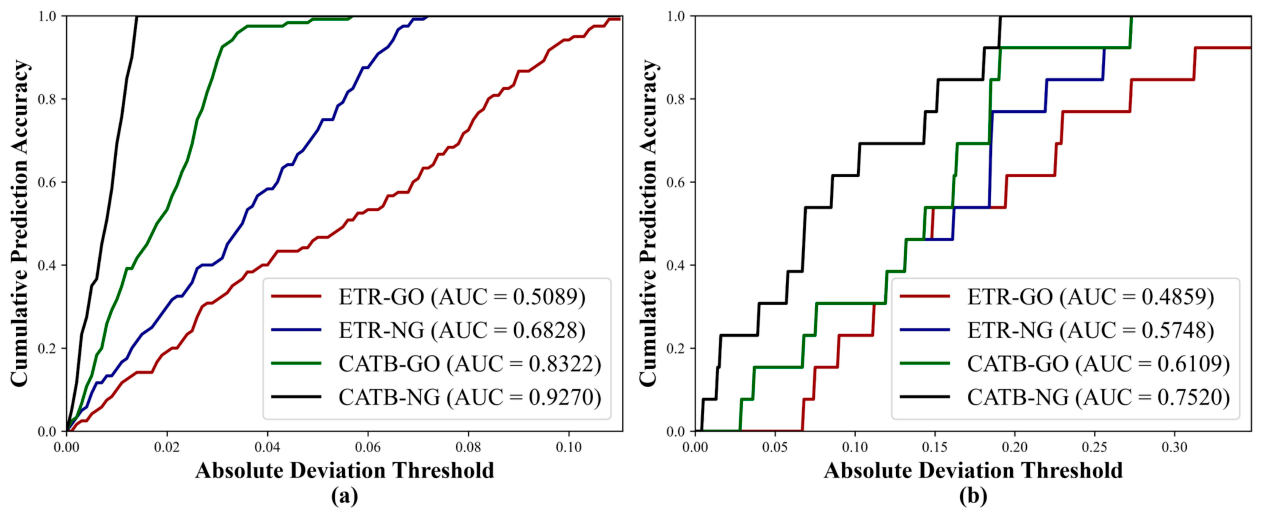
The performance of all the models across different metrics is not enough. So, other performance metrics are crucially needed to understand the error distribution and the computational time. The regression error characteristic (REC) curve is a statistical method for performance evaluation of regression models [73]. The REC curve plots accuracy (the fraction of predictions within some acceptable error of the actual value) against absolute deviation (the absolute impact of the prediction and actual values). For the REC, the Area Under the Curve (AUC) assesses how well our model identifies the right elements. It is expected that the AUC score will increase in the case of a more reliable and stable model with fewer errors in predictions. Also, this metric is very helpful in evaluating how well models generalize because it graphically shows the distribution of the errors at different tolerance levels.
From a training perspective, as shown in Figure 6a, CATB-NG (AUC = 0.9270) shows the highest accuracy among all the error tolerance intervals and the best learning capacity with the lowest error margin on this dataset. The comparatively less predictive accuracy of the CATB model is reflected in the use of genetic variation in the form of the CATB-GO model, which achieved an AUC of 0.8322. Although CATB-GO has a high degree of predictive accuracy, it still performs slightly worse than the non-genetic-based model. Within the ETR solution, ETR-NG (AUC = 0.6828) significantly outperforms ETR-GO (AUC = 0.5089), indicating that the non-genetic optimization method reduces the error effectively during training of the ETR model. The low performance of ETR-GO (~0.51) also indicates that there is a problem in either hyperparameter tuning or overfitting, as most predictions from the training phase show a high deviation. The trend of the REC curve shows agreement with previously observed behavior of the training sets, confirming that CATB-NG has the best accuracy and the smallest absolute deviations, as shown in Figure 6b. All AUC values decline when testing the models when applied to new (unseen) data. This will reduce the estimates of generalization ability. However, CATB-NG (AUC = 0.7520), which is the most accurate model, continues to exhibit robust predictive power with a reduced error rate. Although the CATB-GO (AUC = 0.610) model is ranked in second place, its generalization is not as good as training. Among the ETR, ETR-NG (AUC = 0.5748) comes out on top compared to ETR-GO (AUC = 0.4859), further reinforcing the idea that the model without genetic information is better equipped to minimize error on test data. Despite the decline in AUC values for all models, there is an increase in the error distribution on unseen data. This is not always sufficient, but still, CatB models always outperform ETR, confirming their robustness. The analysis based on AUC demonstrates that CATB-NG is the most robust, as it achieves the best balance between accuracy and minimizing deviations in both training and test samples.
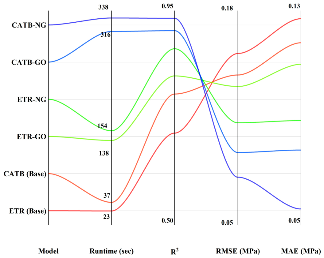
Likewise, Figure 7 is a technical summary of all models, taking both computational overhead and prediction quality into account and evaluating them using runtime, R2, RMSE, and MAE concurrently. The runtime is an indication of the time required to train and optimize the models, thus addressing algorithmic complexity. Predictive performance is also expressed in R2, the proportion of variance explained, along with RMSE and MAE for absolute and average prediction errors in MPa. Smaller RMSE and MAE reflect narrower error distributions, whereas a larger R2 reflects higher predictive consistency. The visual trends clearly indicate a hierarchy from base to optimized hybrids in improving accuracy, which progresses systematically at the cost of computational efforts.
The reference performance levels are set using the base models. ETR (Base) exhibits the smallest runtime (23 s) but also the poorest prediction performance (R2 = 0.695, RMSE = 6.602 MPa, and MAE = 4.621 MPa). These results suggest a low capture of variance and high prediction-error dispersion. CATB Base performance enhancement takes place, with R2 increasing from 0.533 to 0.764 and error decreasing to an RMSE of 5.828 MPa and MAE of 4.079 MPa, accompanied by a small runtime increase to approximately 37 s. This also supports the stronger learning ability of gradient boosting over ensemble tree regression without external optimization. However, the base models are hindered by poor parameter tuning, which narrows their generalization accuracy.
The performance improvements of the optimized models are significant and quantifiable. For ETR, with GO, the R2 of 0.695 is improved to an R2 of 0.813 by optimization and further to an R2 of 0.870 by NG. Likewise, RMSE decreases from 6.602 to 5.203 and then to 4.330 MPa while MAE decreases from 4.621 to 4.282 and then to 3.457 MPa as well. These are obtained with an average increase in running time to 138 s and 154 s. The hybrids based on CATB are the most enhanced. The CATB GO can increase R2 from 0.902 to 0.908 and decrease RMSE/MAE down to 3.654 MPa/3.034 MPa, respectively. CATB NG attains the best predictive performance with an R2 of 0.934 and RMSE and MAE of 3.081 MPa and 2.186 MPa in terms of accuracy with a running time of 338 s. From a research point of view, when prioritizing prediction reliability and error minimization, CATB NG shows an optimal trade-off; otherwise, ETR NG is a good alternative solution with reasonable computational cost.

5.3. SHAP and ICE-Based Model Explainability

SHapley Additive exPlanations (SHAP) is an advanced model interpretability technique rooted in cooperative game theory that is used to quantify each feature’s contribution to a model’s predictions [74,75,76]. SHAP values quantify the contribution of each feature by calculating the change in the model’s prediction when that feature is added or removed. SHAP values can be positive (i.e., they have added value to the predicted output) or negative (i.e., this particular feature reduces the predicted output), meaning that SHAP can be used for both regression and classification. SHAP is especially beneficial for complex machine learning models like gradient boosting and ensemble methods, which do not offer directly interpretable parameters the way linear models’ coefficients do.
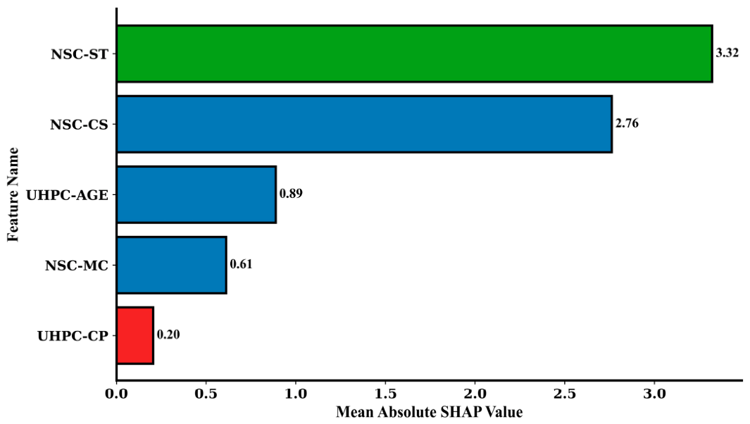
The feature importance plot explains variables based on their mean absolute SHAP values, describing their overall contribution to model predictions as presented in Figure 8. According to this plot, the NSC-ST has the highest mean SHAP value (3.32), reflecting its crucial role in bond strength predictive capabilities. Also, NSC-CS follows a mean SHAP value of 2.76, which further confirms its strong contribution. In the meantime, UHPC-AGE (0.89) and NSC-MC (0.61) act as relatively moderate contributors, whereas UHPC-CP (0.20) has the least impact on model predictions. The drastic difference between NSC-ST and other parameters is the indication that surface treatment is a prominent feature in predicting the bond strength, whereas curing is found to have a lesser impact (UHPC-CP). That indicates that surface treatment should receive more focus in model optimization.
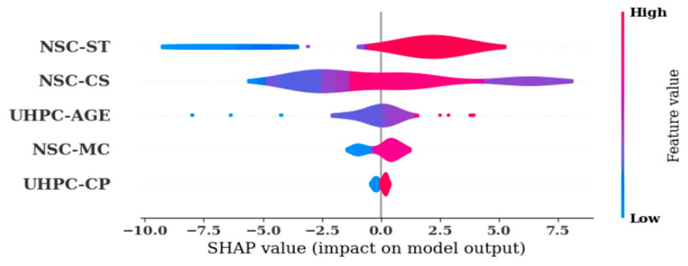
The summary plot shows SHAP values for all data points in a single figure, providing a sense of the impact and distribution of each feature as presented in Figure 9. In the plot, the x-axis represents SHAP values, which reflect each feature’s influence on model output, whereas feature magnitude is shown in a color gradient with blue representing the lower values and red representing the higher values. The widespread use of SHAP values for NSC-ST highlights that it has the most dominant effect on predictions. A high-density of points is observed around the positive SHAP values. This suggests that a higher level of surface treatment contributes positively to bond strength. NSC-CS, in contrast, has a large spread, indicating that the SHAP values are relatively evenly distributed between the positive and negative. This implies that NSC-CS has a different importance for different samples. On the other hand, UHPC-CP is very confined in terms of SHAP values, which further confirms its low predictive importance. The heatmap shows that high values of NSC-ST and NSC-CS tend to raise predictions, as expected, while low values negatively affect predictions.
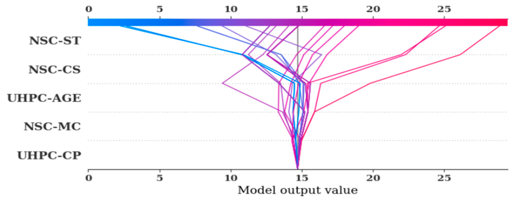
The SHAP decision plot gives an in-depth view of the contributions of the features cumulatively to the prediction of the model presented in Figure 10. Each line indicates a single prediction, demonstrating how SHAP values adjust the output of the model. This again shows NSC-ST as the largest discrepancy, significantly influencing the bond strength prediction. The line split accordingly at a number of features, indicating more of an impact on some samples than on others. A similar rough pattern is observed with NSC-CS, but with lower variance. The bond strength increases with increasing SHAP values for NSC-ST, while the results decrease with a lower SHAP value. UHPC-CP shows low variability, which means that predictions are not very dependent on curing process settings. The color gradient in the top bar is a visual indication of bond strength, with a darker color representing higher predictions of bond strength. This also shows that the predictions of the model are predominantly driven by NSC-ST and NSC-CS, while other features have much less of an impact.
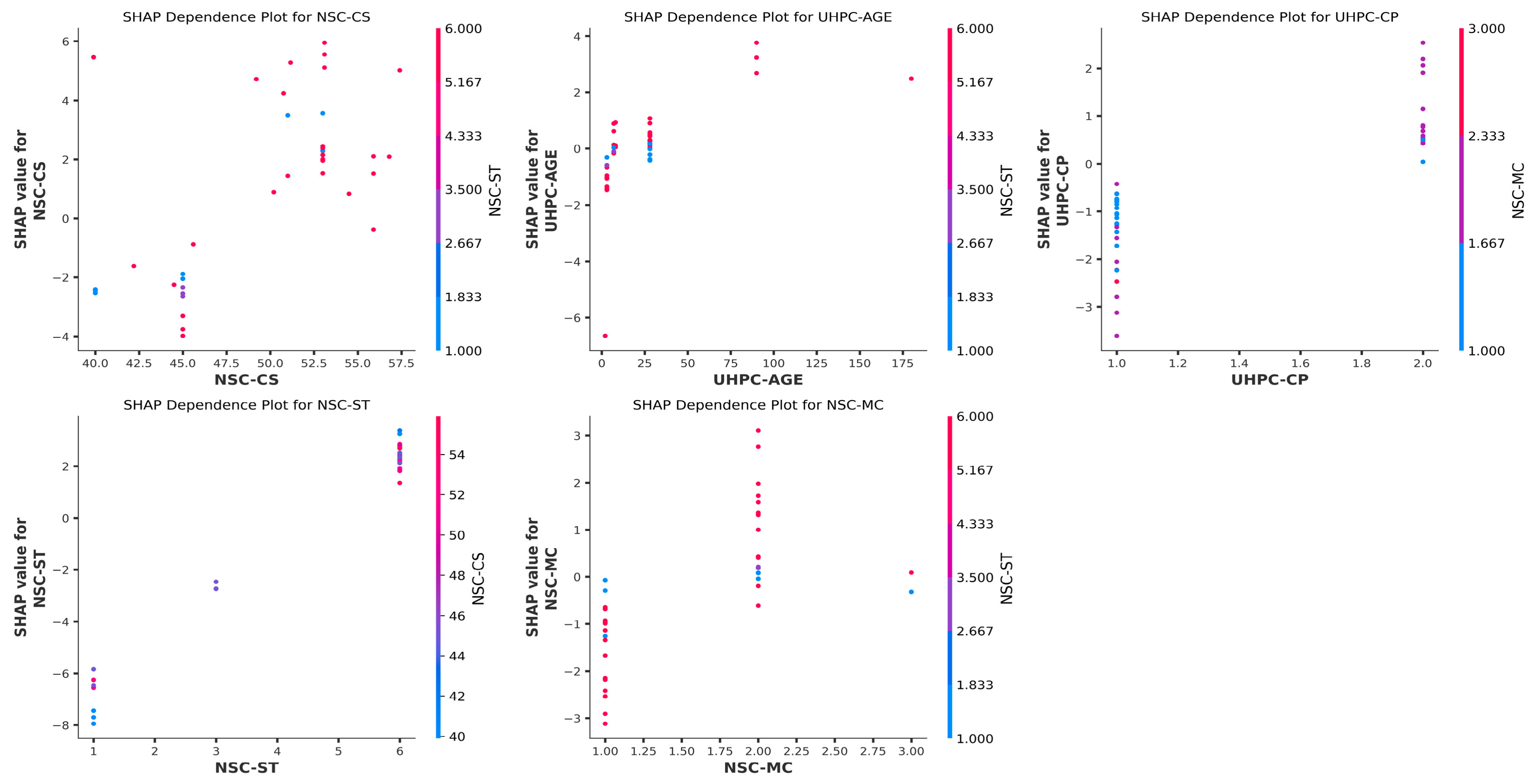
The SHAP dependence plot shows how each feature influences the predictions of the model (SHAP values) and interaction effects with secondary features presented in Figure 11. In each subplot, the x-axis represents a specific feature, while the y-axis represents its respective SHAP values, showing its contribution to the model’s output (BS). It also serves as an interacting feature, which is represented by the color gradient, to give an idea of how the two features (weight and height) are dependent on each other. In other words, NSC-ST (surface treatment) shows the strongest impact, while its SHAP values vary from nearly −4 to +6, indicating a direct relationship between elevated NSC-ST values and augmented bond strength. The dependence plot for NSC-CS (compressive strength) shows a similarly large spread (−4 to +6 SHAP values), which demonstrates that a higher compressive strength results in a significant positive effect on the bond strength. As shown by the color gradient, interaction effects show that NSC-ST also strengthens the effect of NSC-CS. The SHAP values in the UHPC-AGE plot show a more concentrated range (−6 to +4), indicating that age has a moderate but very variable impact, with higher values predominantly increasing bond strength. The NSC-MC plot shows that lower moisture content results in a minuscule negative effect on NSC-MC predictions with a SHAP value of −3 and a high moisture content of 3.0, which shows a neutral or slightly positive effect, but still no visible impact. Lastly, UHPC-CP (curing process) also exhibited the best behavior and a small range of SHAP values (−3 to +2), further confirming its lesser influence in model predictions. The analysis of interaction shows that NSC-ST and NSC-CS dominate the model’s decision-making process, followed by UHPC-AGE, NSC-MC, and UHPC-CP. The detailed analysis shows that the surface treatment and compressive strength play the most important role, and their interaction significantly determines the predicted bond strength.
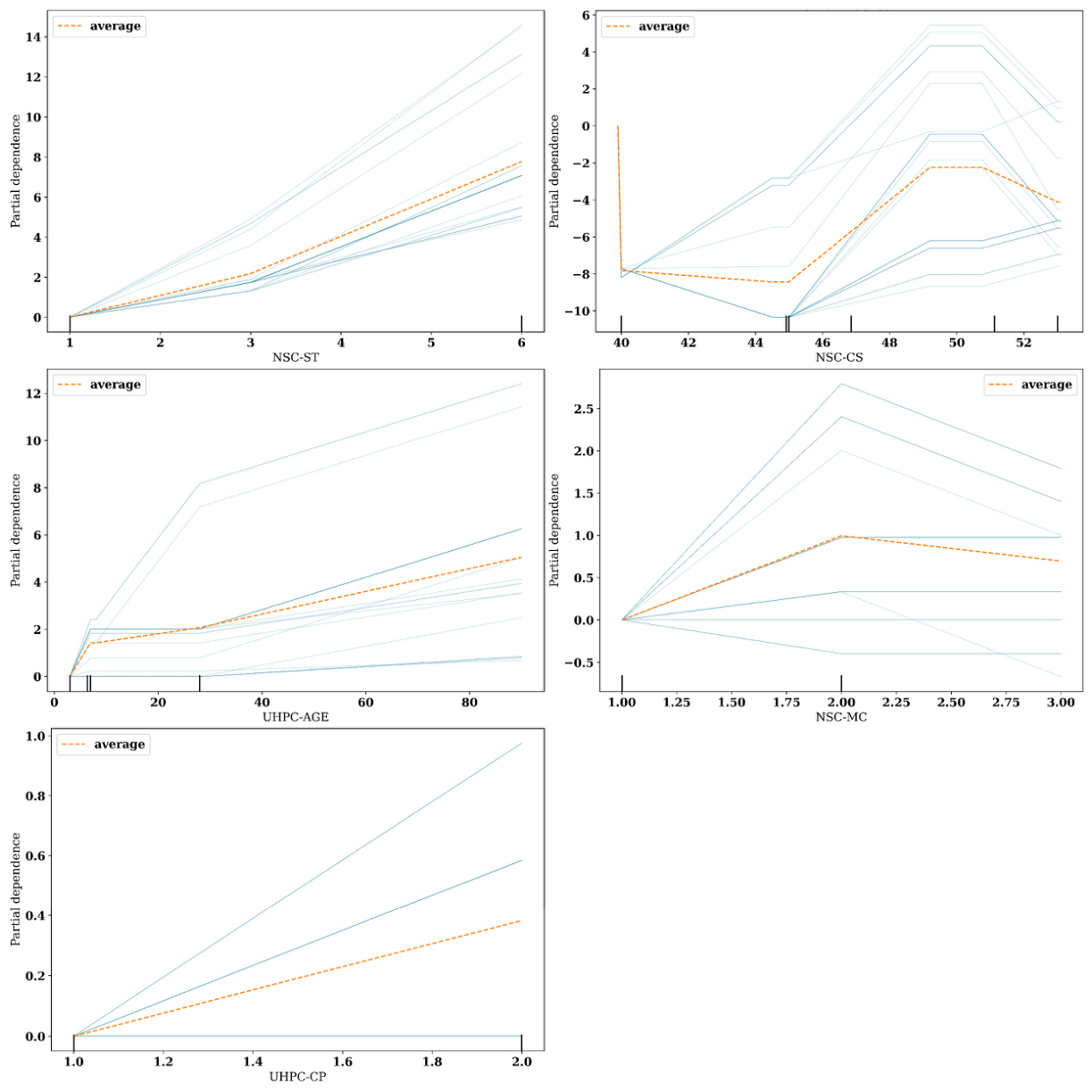
An Individual Conditional Expectation plot (ICE plot) is a graphical display that allows one to observe how a model’s predictions would vary when individual feature values are modified, while taking the variance over many observations into account [77,78]. The ICE plot result is presented in Figure 12. The light blue lines represent a unique data instance, demonstrating the independent effect that the feature value has on predicted bond strength. The average between all partial dependencies is shown by the dashed orange line that summarizes the overall trend. The ICE plots for NSC-ST and NSC-CS also show a strong and nonlinear dependence of these descriptors on bond strength. For NSC-ST, as the surface treatment value continues to increase, the predictions increase proportionately, but it is generally seen that the effects have the strongest influence above a value of 3. This trend remains consistent across all data points, solidifying NSC-ST as the most predictive one. The trend of NSC-CS appears to be nonlinear: between 40 and 46 MPa, the bond strength decreases significantly, only to increase beyond this point, indicating that it potentially interacts with other variables. However, for UHPC-AGE, a positive correlation was determined, with some sharper increases in bond strength for the first values (0–20 days), while later (beyond 40 days), no changes can be found. This indicates that longer curing times cause greater strength, but eventually that would plateau. NSC-MC has a weak linear relationship with slightly nonlinear behavior around a lower limit between 1.5 and 2.5, with a higher potential impact, peaking at a certain point, and then declining below 2.5. The ICE curves show variability in these observations, indicating some interaction with other factors. In contrast, UHPC-CP showed a less pronounced and linear effect on bond strength. The instances have very low variability, thus further confirming that UHPC-CP does not significantly influence the model’s predictions. These ICE plots affirm that NSC-ST and NSC-CS dominate, while there is a secondary influence, specifically from both UHPC-AGE and NSC-MC, leaving little to no effect from UHPC-CP.

5.4. Discussion and Graphical User Interface

The evaluation of predictive performance is demonstrated in Table 4, comparing the proposed framework with previous machine learning studies utilizing the same slant shear bond strength dataset. The comparison illustrates a very clear improvement in prediction accuracy obtained by the present work relative to previous approaches. Faroukh and Jinsong [39] used a Random Search-tuned SVM, which resulted in a testing R2 of 0.792 with an RMSE of 3.465 MPa. Despite the model capturing reasonable predictive power, the performance of this classic machine learning algorithm was limited by its inability to handle the strongly nonlinear relationships among governing material, mixture and interface parameters. Subsequently, Sapkota et al. [42] achieved an additional extension for the predictive framework by implementing the CatBoost algorithm with Bayesian hyperparameter optimization, completed with SHAP and ICE analyses for better model interpretability. Gradient boosting and explainable artificial intelligence (XAI) demonstrated their benefits by providing a better understanding of the influential variables. This approach also improved the testing performance, achieving an R2 of 0.8274 and an RMSE of 3.1375 MPa.
Based on these advancements, the current study presents an ensemble–metaheuristic framework combining CatBoost with GO and NG. Contradicting previous findings, the proposed framework not only minimizes the hyperparameter search problem using bio-inspired optimization algorithms but presents a systematic comparison of four hybrid models to select the most robust predictive structure across different datasets. The optimal CATB-NG model obtained a testing R2 of 0.934 and RMSE of 2.186 MPa, which corresponds to an approximately 17.9% improvement in accuracy compared to the SVM model, and also an approximately 13.0% enhancement compared to the Bayesian-optimized CatB model. Likewise, it made considerable improvements with RMSE reducing by 36.9% and 30.3%. The better predictive performance comes from the GO and NG algorithms having preferable exploration and exploitation ability compared to those in traditional optimization methods, allowing for less intensive but more effective hyperparameter tuning. In addition, combining SHAP and ICE provided global and local interpretability of the built models, while building a GUI improves the pragmatic applicability of the proposed framework in engineering practice. This combination of improvements shows that the proposed framework not only has much better accuracy in predication but is also more transparent and practical to use, making it a series-step advance over existing machine learning methods for UHPC-NSC slant shear bond strength prediction.
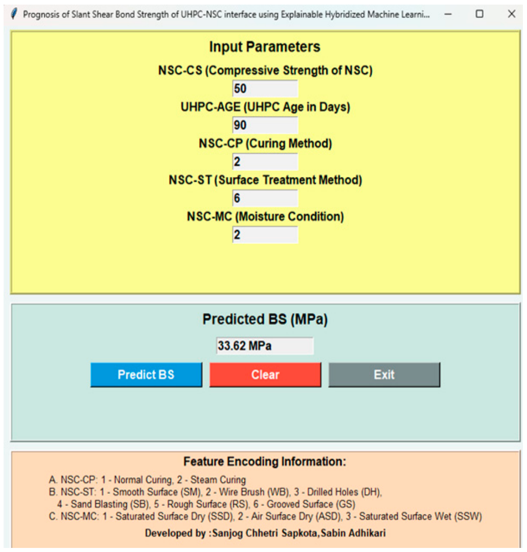
This graphical user interface (GUI) was developed using the Tkinter framework available within the Python standard library [79]. It is effective for the prediction of slant shear bond strength (BS) at the UHPC-NSC interface employing an explainable hybridized machine learning model as shown in Figure 13. It combines important factors’ influences to accurately determine bond strength, including those of NSC-CS, UHPC-AGE, NSC-CP, NSC-ST, and NSC-MC. Users can thus enter these variables into the system to be able to take advantage of an optimized predictive model trained on a large dataset covering different curing, treatment, and aging conditions. This considers the surface preparation techniques and curing environments, all of which can influence interfacial bond performance. After entering the input parameters, once the user retrieves the BS in megapascals (MPa), the GUI will help researchers and engineers in assessing UHPC-NSC bond performance, significantly improving the efficiency in the process of analysis and experimentation. Moreover, this tool is useful for mix optimization and the assessment of structural retrofitting solutions, as well as performance-based design of composite UHPC-NSC structures, serving as a rapid and efficient procedure to predict the interface bond strength experienced under distinct preparation and curing conditions.
Although the developed hybridized approach is more accurate in predicting interfacial bond strength between UHPC and NSC, some limitations should be considered. The primary limitation is the small size of the dataset (there were fewer than 150 data samples). Small sample sizes lead to statistical weakness of models and poor generalization properties in unseen or extreme conditions. It can also be observed, however, that the relationship among physical factors, including surface treatment type, curing method/moisture state, UHPC age, etc., is inherently nonlinear and very sensitive to local boundary conditions. Even small experimental or environmental perturbations (temperature, humidity, and perhaps casting sequence) introduce large variations in the measured bond strength that current models do not adequately describe. Moreover, although the use of bio-inspired optimizers such as GO and NG improves parameter tuning considerably, these techniques are still expensive to compute. They may be trapped in suboptimal solutions if perturbed by noise in objective function evaluations or by high-dimensional spaces. The lack of information about real-time or probabilistic uncertainty quantification also hinders the model from expressing confidence in its own forecast, a necessity for high-stakes structural design use cases.
In future work, developing data fusion from multiple sources/laboratories/simulations, or applying data augmentation at the laboratory scale, could significantly enhance model stability and coverage. Such a consideration can be effectively incorporated into data-driven models via PIML frameworks to avoid the discrepancy with known material behavior. In addition, uncertainty-aware models and active learners, including Bayesian ensembles, conformal regressors, and epistemic–aleatoric hybrid learners, can be used to self-assess reliability and decide which data points to query from the most uncertain regions. Moreover, domain adaptation and transfer learning can be added to generalize predictions to new materials, geometries, or curing regimes. In terms of computation, it is interesting to investigate multi-objective optimization considering accuracy, interpretability, and runtime efficiency. Also, the creation of interactive and cloud-embedded analytics platforms would enable researchers and practitioners to visualize model outputs, interpret sensitivity analysis under SHAP and ICE framework conditions, as well as apply trained models to practical decisions at a design level. Together, these extensions will be to the benefit of the scientific and engineering community in terms of the relevance of machine learning tools in interfacial bond characterization.

6. Conclusions

This paper describes a robust and application-driven machine learning framework for the prediction of slant shear bond strength at the UHPC-NSC interface that overcomes the deficiencies of traditional empirical and data-driven ways to capture nonlinear and interaction-based responses. The system consolidates ensemble learning, bio-inspired optimization, and explainable artificial intelligence to gain enhanced predictive power at a consistent physical understanding level. The incorporation of computational efficiency evaluation and GUI-based implementation further evidences the balance between accuracy and practical utilities, which allows informed decision making in UHPC NSC composite design and retrofitting.
  • The hybrid models, when optimized, demonstrate a clear increase in predictive power over the base learners. The test set R2 value rises gradually from 0.695 and 0.764 in ETR Base and CATB Base to 0.870 and 0.934 in ETR NG and CATB NG, respectively. Meanwhile, RMSE decreases from 6.602 MPa and 5.828 MPa to 4.330 MPa and 3.081 MPa, while MAE reduces from 4.621 MPa and 4.079 MPa to 3.457 MPa and 2.186 MPa. These gains support strong generalization and a compact error bound for the optimized model.
  • Base models offer the fastest runtime, with 23 s in the case of ETR and 37 s for CATB, but weak prediction accuracy. In the case where hybridization with GO and NG is used, the runtime increases in the range of 138 s to 338 s, but these lead to large improvements in performances. ETR-NG enhances R2 by approximately 25% (at the cost of up to 6.7 times the runtime). Furthermore, CATB-NG enhances R2 by approximately 22%, at the cost of an approximately 9.1-fold increase in runtime. This is an explicit accuracy computation trade-off.
  • The NSC surface treatment is shown to be the dominant factor over bond strength, according to the SHAP results. It reveals that the UHPC age and moisture condition have a medium-scale effect, and the curing manner is of little importance. These trends are consistent with a bond transfer mechanism that is controlled by the mechanical interlocking and coercer integrity.
  • Trends of SHAP dependence show that NSC with a rough or mechanically treated surface is associated with higher bond strength. Enhanced NSCs appear to improve bond performance up to a saturation level, after which further benefits diminish. The age of the UHPC has a threshold effect and is significant in that it develops rapidly at its early ages, then reaches stability.
  • The SHAP dependence plot shows that typically the roughed or mechanically treated NSCs are the highest positive SHAP values, indicating they make good candidates for bond improvement. The CS of NSC contributes positively to an optimal mid-to-high strength range, past which the marginal increase in bond strength becomes smaller. There exists a threshold effect in the bond properties of UHPC with a substantial increase at early to mid-age, followed by stabilization. SHAP contributions are always higher under lower moisture conditions, and this may reflect greater interfacial adhesion at these reduced levels of surface moisture.
  • The ICE plots indicate strong nonlinear and interaction effects, especially between surface treatment and NSC strength. Only when both parameters are favorably aligned does the bond strength increase steeply, which accounts for the range of applicability of linear or weak sequence-dependent models.
  • A GUI of the user interface is developed by using Tkinter with an implemented optimized CATB-NG model for live prediction. The framework maintains stable feature representation, stationary inference, and fast bond strength evaluation in the face of uncertainties, enabling practical engineering decision making without requiring expertise in machine learning.

Author Contributions

Conceptualization, methodology, formal analysis, software, data curation, visualization, S.C.S.; investigation, S.C.S., N.P., and S.P. (Sandip Pandey); methodology, S.A. and K.K.; software, S.A.; resources, N.P. and B.L.; validation, N.P. and K.K.; writing—original draft preparation, S.C.S., N.P., B.L., S.P. (Sandip Pandey), and K.K.; writing,—review and editing, S.C.S., S.A., N.P., B.L., S.P. (Sandip Pandey), K.K., and S.P. (Satish Paudel); supervision and project administration, S.P. (Satish Paudel); conceptual guidance, S.P. (Satish Paudel). All authors have read and agreed to the published version of the manuscript.

Funding

This research received no external funding.

Data Availability Statement

The data that support the findings of this study are available from the corresponding author upon reasonable request.

Conflicts of Interest

The authors declare no conflicts of interest.

References

  1. Mizan, M.H.; Hayakawa, R.; Matsumoto, K. Effects of Combined Deterioration of Steel Corrosion and Freeze-Thaw Cycles on the Pull-Out Behavior of Deformed Bars in Concrete. Constr. Build. Mater. 2025, 505, 144758. [Google Scholar] [CrossRef] [Scilit]
  2. Zhang, J.; Li, J.; Yun, H.; Long, J.; Zhu, Q.; Guan, Z. Durability of New-to-Old Concrete Interface under Coupling Action of Freeze-Thaw Cycle and Chloride Salt Erosion. Structures 2024, 70, 107867. [Google Scholar] [CrossRef] [Scilit]
  3. Khan, M.B.; Abbas, Y.M.; Shafiq, N.; Khan, M.I.; Zahid, M.; Masmoudi, R. Stress Transformation at Slant Interfaces in Concrete Structures: Role of Graphene Enhanced Fiber Overlays in Building Rehabilitation. J. Build. Eng. 2025, 113, 114019. [Google Scholar] [CrossRef] [Scilit]
  4. Huang, T.; Bobyr, M. Review of Delamination Damage of Composite Materials. J. Compos. Sci. 2023, 7, 468. [Google Scholar] [CrossRef] [Scilit]
  5. Amran, M.; Huang, S.S.; Onaizi, A.M.; Makul, N.; Abdelgader, H.S.; Ozbakkaloglu, T. Recent Trends in Ultra High Performance Concrete: Current Status, Challenges, and Future Prospects. Constr. Build. Mater. 2022, 352, 129029. [Google Scholar] [CrossRef] [Scilit]
  6. Bahmani, H.; Mostafaei, H.; Santos, P.; Fallah Chamasemani, N. Enhancing the Mechanical Properties of Ultra High Performance Concrete through Silica Sand Replacement with Steel Slag. Buildings 2024, 14, 3520. [Google Scholar] [CrossRef] [Scilit]
  7. Akhnoukh, A.K.; Buckhalter, C. Ultra High Performance Concrete: Constituents, Mechanical Properties, Applications and Current Challenges. Case Stud. Constr. Mater. 2021, 15, e00559. [Google Scholar] [CrossRef] [Scilit]
  8. Shrestha, A.; Sapkota, S.C. Hybrid machine learning model to predict the mechanical properties of ultra-high-performance concrete (UHPC) with experimental validation. Asian J. Civ. Eng. 2024, 25, 5227–5244. [Google Scholar] [CrossRef] [Scilit]
  9. Wang, X.; Ma, Z.; Wang, X.; Xue, S.; Shen, W.; Wu, D.; Zhang, X.; Han, Z.; Sui, S.; Wang, M.; et al. Design of Self-Compacting Ultra High Performance Concrete towards Cementitious Materials Packing Optimization. Cem. Concr. Compos. 2024, 148, 105443. [Google Scholar] [CrossRef] [Scilit]
  10. Xu, Z.; Qin, F.; Yang, Q.; Peng, X.; Xu, B. Review of Research on the Interfacial Shear Performance of Ultra High Performance Concrete and Normal Concrete Composite Structures. Coatings 2025, 15, 414. [Google Scholar] [CrossRef] [Scilit]
  11. Bai, M.; Ding, T.; Zhao, Y.; Zhao, Y. Shear Performance of New-to-Old Concrete Interface Based on Various Surface Preparation Techniques and Roughness. Case Stud. Constr. Mater. 2024, 21, e03549. [Google Scholar] [CrossRef] [Scilit]
  12. Zhang, B.; Yu, J.; Chen, W.; Liu, H.; Li, H.; Guo, H. Experimental Study on Bond Performance of NC-UHPC Interfaces with Different Roughness and Substrate Strength. Materials 2023, 16, 2708. [Google Scholar] [CrossRef] [Scilit] [PubMed]
  13. Fan, T.; Xu, P.; Chen, H.; Yuan, T.; Xu, A.; Chen, C.; Wu, Y. Analysis of Surface Texture Distribution Characteristics of Concrete Substrate and Modeling of Coating Adhesion Strength. Materials 2025, 18, 5412. [Google Scholar] [CrossRef] [Scilit] [PubMed]
  14. Tayeh, B.A.; Abu Bakar, B.H.; Megat Johari, M.A.; Voo, Y.L. Mechanical and Permeability Properties of the Interface between Normal Concrete Substrate and Ultra High Performance Fiber Concrete Overlay. Constr. Build. Mater. 2012, 36, 538–548. [Google Scholar] [CrossRef] [Scilit]
  15. Farouk, A.I.B.; Rong, W.; Zhu, J. Compressive Behavior of Ultra High Performance Concrete-Normal Strength Concrete Column with the Longitudinal Grooved Contact Surface. J. Build. Eng. 2023, 68, 106074. [Google Scholar] [CrossRef] [Scilit]
  16. Horák, P.; Pešková, Š.; Jogl, M.; Sovják, R.; Vítek, P. Experimental Investigation of Cohesion between UHPC and NSC Utilising Interface Protrusions. Materials 2022, 15, 6537. [Google Scholar] [CrossRef] [Scilit] [PubMed]
  17. Santos, D.S.; Santos, P.M.D.; Dias da Costa, D. Effect of Surface Preparation and Bonding Agent on the Concrete-to-Concrete Interface Strength. Constr. Build. Mater. 2012, 37, 102–110. [Google Scholar] [CrossRef] [Scilit]
  18. Daneshvar, D.; Behnood, A.; Robisson, A. Interfacial Bond in Concrete-to-Concrete Composites: A Review. Constr. Build. Mater. 2022, 359, 129195. [Google Scholar] [CrossRef] [Scilit]
  19. Zhang, Y.; Zhu, P.; Wang, X.; Wu, J. Shear Properties of the Interface between Ultra High Performance Concrete and Normal Strength Concrete. Constr. Build. Mater. 2020, 248, 118455. [Google Scholar] [CrossRef] [Scilit]
  20. Haber, Z.B.; Munoz, J.F.; de la Varga, I.; Graybeal, B.A. Bond Characterization of UHPC Overlays for Concrete Bridge Decks: Laboratory and Field Testing. Constr. Build. Mater. 2018, 190, 1056–1068. [Google Scholar] [CrossRef] [Scilit]
  21. Feng, S.; Xiao, H.; Liu, R.; Liu, M. Bond Properties between Ultra High Performance Concrete and Normal Strength Concrete Substrate: Bond Macro Performance and Overlay Transition Zone Microstructure. Cem. Concr. Compos. 2022, 128, 104436. [Google Scholar] [CrossRef] [Scilit]
  22. Xu, L.; Yao, Y.; Li, Y.; Su, J.; Wu, Y. Review of the Interfacial Bonding Properties between Ultra High Performance Concrete and Normal Concrete. Appl. Sci. 2023, 13, 6697. [Google Scholar] [CrossRef] [Scilit]
  23. Muñoz, M.A.C.; Harris, D.K.; Ahlborn, T.M.; Froster, D.C. Bond Performance between Ultra High Performance Concrete and Normal Strength Concrete. J. Mater. Civ. Eng. 2014, 26, 04014031. [Google Scholar] [CrossRef] [Scilit]
  24. Lessly, H.S.; Kumar, S.L.; Jawahar, R.R.; Prabhu, L. Durability Properties of Modified Ultra High Performance Concrete with Varying Cement Content and Curing Regime. Mater. Today Proc. 2021, 45, 6426–6432. [Google Scholar] [CrossRef] [Scilit]
  25. Khaksefidi, S.; Ghalehnovi, M.; de Brito, J. Bond Behaviour of High Strength Steel Rebars in Normal Strength Concrete and Ultra High Performance Concrete. J. Build. Eng. 2021, 33, 101592. [Google Scholar] [CrossRef] [Scilit]
  26. Huang, H.; Yuan, Y.; Zhang, W.; Liu, B.; Viani, A.; Mácová, P. Microstructure Investigation of the Interface between Lightweight Concrete and Normal Weight Concrete. Mater. Today Commun. 2019, 21, 100640. [Google Scholar] [CrossRef] [Scilit]
  27. Kahangi Shahreza, S.; Ahmadi, K. Data-Driven Prediction of Masonry Flexural Bond Strength: Interpretability and Implications. Case Stud. Constr. Mater. 2025, 23, e05412. [Google Scholar] [CrossRef] [Scilit]
  28. Liu, T.; Pan, C.; Huang, T.; Ai, Y.; Xu, Z.; Li, J.; He, Z.; Xie, M. Hybrid Parameter-Driven Analysis-Based Approach for Predicting the Interface Bond Strength between Steel Bar and Machine-Made Gravel Aggregate Concrete. Case Stud. Constr. Mater. 2025, 23, e05325. [Google Scholar] [CrossRef] [Scilit]
  29. Muftuoglu, G.M.; Dehghanian, K. Soil Liquefaction Assessment Using Machine Learning. Artif. Intell. Geosci. 2025, 6, 100122. [Google Scholar] [CrossRef] [Scilit]
  30. Mengistu, T.D.; Chung, I.-M.; Chang, S.W. Machine Learning for Water Quality Prediction and Uncertainty Assessment. Phys. Chem. Earth 2026, 143, 104319. [Google Scholar] [CrossRef] [Scilit]
  31. Shah, S.M.T.; Piantanakulchai, M. Ensemble Machine Learning for Travel Time Prediction: An Active Learning-Assisted Approach. Results Eng. 2026, 29, 108712. [Google Scholar] [CrossRef] [Scilit]
  32. Abduljabbar, R.; Dia, H.; Liyanage, S. Machine Learning Traffic Flow Prediction Models for Smart and Sustainable Traffic Management. Infrastructures 2025, 10, 155. [Google Scholar] [CrossRef] [Scilit]
  33. Chomacki, L.; Rusek, J.; Słowik, L. Machine Learning in Predicting Failures of Buried Water Supply Networks Affected by Mining Impacts. Sci. Rep. 2026, 16, 8465. [Google Scholar] [CrossRef] [Scilit] [PubMed]
  34. Liu, Y.; Luo, H. An Efficient Machine Learning-Based Model for Duration Prediction of Construction Tasks with Large-Scale Datasets. Adv. Eng. Inform. 2026, 69, 103820. [Google Scholar] [CrossRef] [Scilit]
  35. Özkılıç, Y.O.; Ecemis, A.S.; Stel’Makh, S.A.; Beskopylny, A.N.; Shcherban’, E.M.; Yildizel, S.A.; Aksoylu, C.; Madenci, E. Thermo-Mechanical and Data-Driven Assessment of Sustainable Concrete Incorporating Waste Tire Aggregates and Recycled Steel Fibers. Buildings 2026, 16, 946. [Google Scholar] [CrossRef] [Scilit]
  36. Zhang, F.; Wang, C.; Liu, J.; Zou, X.; Sneed, L.H.; Bao, Y.; Wang, L. Prediction of FRP-Concrete Interfacial Bond Strength Based on Machine Learning. Eng. Struct. 2023, 274, 115156. [Google Scholar] [CrossRef] [Scilit]
  37. Su, M.; Zhong, Q.; Peng, H.; Li, S. Selected Machine Learning Approaches for Predicting the Interfacial Bond Strength between FRPs and Concrete. Constr. Build. Mater. 2021, 270, 121456. [Google Scholar] [CrossRef] [Scilit]
  38. Hiew, S.Y.; Teoh, K.B.; Raman, S.N.; Kong, D.; Hafezolghorani, M. Prediction of Ultimate Conditions and Stress-Strain Behaviour of Steel-Confined Ultra-High-Performance Concrete Using Sequential Deep Feed-Forward Neural Network Modelling Strategy. Eng. Struct. 2023, 277, 115447. [Google Scholar] [CrossRef] [Scilit]
  39. Farouk, A.I.B.; Zhu, J. Prediction of Interface Bond Strength between Ultra High Performance Concrete and Normal Strength Concrete Using a Machine Learning Approach. Arab. J. Sci. Eng. 2022, 47, 5337–5363. [Google Scholar] [CrossRef] [Scilit]
  40. Lazaridis, P.C.; Thomoglou, A.K. Rapid Shear Capacity Prediction of TRM-Strengthened Unreinforced Masonry Walls through Interpretable Machine Learning Deployed in a Web App. J. Build. Eng. 2024, 98, 110912. [Google Scholar] [CrossRef] [Scilit]
  41. Gray, D.T.; Simwanda, L.; Sifan, M.; Poologanathan, K.; Kannan, T. Machine Learning Prediction of Shear Strength in Cold-Formed Steel Modular Construction-Optimised (MCO) Beam. Buildings 2026, 16, 1497. [Google Scholar] [CrossRef] [Scilit]
  42. Sapkota, S.C.; Sapkota, S.; Bansal, T.; Haq, M.; Al Osta, M.A. Leveraging Interpretable Ensemble Machine Learning for Predicting Interfacial Bond Strength between Normal Strength Concrete Substrate and UHPC Overlays. Arab. J. Sci. Eng. 2025, 50, 8621–8645. [Google Scholar] [CrossRef] [Scilit]
  43. Liu, K.; Wu, T.; Shi, Z.; Yu, X.; Lin, Y.; Chen, Q.; Jiang, H. Interpretable Machine Learning Models for Predicting the Bond Strength between UHPC and Normal Strength Concrete. Mater. Today Commun. 2024, 40, 110006. [Google Scholar] [CrossRef] [Scilit]
  44. Tian, L.; Wang, L.; Xian, G. Machine Learning Prediction of Interfacial Bond Strength of FRP Bars with Different Surface Characteristics to Concrete. Case Stud. Constr. Mater. 2024, 21, e03984. [Google Scholar] [CrossRef] [Scilit]
  45. Li, R.; Sun, W.; Wang, J.; Zhan, S.; Zhang, J.; Wang, G. XGBoost Prediction of UHPC-NC Bond Strength Using Interface Damage Parameters. Eng. Fract. Mech. 2026, 338, 112042. [Google Scholar] [CrossRef] [Scilit]
  46. Ecemiş, A.S.; Yildizel, S.A.; Beskopylny, A.N.; Stel’makh, S.A.; Shcherban’, E.M.; Aksoylu, C.; Madenci, E.; Özkılıç, Y.O. Sustainable Concrete with Waste Tire Rubber and Recycled Steel Fibers: Experimental Insights and Hybrid PINN-CatBoost Prediction. Polymers 2025, 17, 2910. [Google Scholar] [CrossRef] [Scilit] [PubMed]
  47. Singh, P.; Singla, S.; Bansal, A.; Kumar, M.; Mrinali, A.; Hasnain, S.M.M. Data-Driven Modeling for Bond Strength in Reinforced Concrete Structures. Sci. Rep. 2026, 16, 16861. [Google Scholar] [CrossRef] [Scilit] [PubMed]
  48. Taffese, W.Z.; Zhu, Y.; Chen, G. Ensemble-Learning Model Based Ultimate Moment Prediction of Reinforced Concrete Members Strengthened by UHPC. Eng. Struct. 2024, 305, 117705. [Google Scholar] [CrossRef] [Scilit]
  49. Mehdizadeh, B.; Fakharian, P.; Nouri, Y.; Afrazi, M.; Samali, B. Machine Learning-Assisted Analysis of Fracture Energy in Externally Bonded Reinforcement on Groove Bond Strength Prediction. Buildings 2026, 16, 1070. [Google Scholar] [CrossRef] [Scilit]
  50. Zhan, S.; Sun, W.; Li, R.; Wang, J.; Zhang, J.; Yang, Y. Prediction and Model Validation of UHPC-NSC Interface Bonding Performance Based on Machine Learning Algorithms. J. Mater. Civ. Eng. 2026, 38, 04025567. [Google Scholar] [CrossRef] [Scilit]
  51. Katlav, M.; Turk, K. Explainable Stacked Machine Learning Models for Predicting Fiber-Reinforced Polymer (FRP) Bars-Concrete Interfacial Bond Strength Retention in Marine Environments. Eng. Struct. 2026, 365, 123237. [Google Scholar] [CrossRef] [Scilit]
  52. Abid, K.A.; Syed, S.A.; Khan, M. Explainable Machine Learning-Based Model for Predicting Interlayer Bond Strength in 3D Printed Concrete. Multiscale Multidiscip. Model. Exp. Des. 2025, 8, 415. [Google Scholar] [CrossRef] [Scilit]
  53. Zhang, Z.; Ge, W.; Han, S.; Ashour, A.; Cao, D.; Wu, J. Genetic Algorithm-Optimized and Explainable Machine Learning for Bond Strength Prediction Between Steel-FRP Composite Bars and Concrete. Eng. Struct. 2026, 359, 122773. [Google Scholar] [CrossRef] [Scilit]
  54. Al-Hamd, R.K.S.; Albostami, A.S.; Warren, H. Data-Driven and Explainable AI Models for Evaluating Bond Strength in Reinforced Concrete at Elevated Temperatures. Fire Saf. J. 2025, 158, 104514. [Google Scholar] [CrossRef] [Scilit]
  55. Kashani, A.H.; Ghalehnovi, M.; Etemadfard, H. ML Modeling of Ultimate and Relative Bond Strength for Corroded Rebars Based on Concrete and Steel Properties. Sci. Rep. 2025, 15, 26830. [Google Scholar] [CrossRef] [Scilit] [PubMed]
  56. Khorshidi, M.; Nejatipour, P.; Teimortashlu, A.; Oliveto, G.; Afaridegan, E. Explainable AI-Based Optimization Framework for Sustainable Fly Ash Concrete Design. Sci. Rep. 2026, 16, 22397. [Google Scholar] [CrossRef] [Scilit] [PubMed]
  57. Nikzad, M.H.; Heidari-Rarani, M.; Sareh, P. From Classical Machine Learning Algorithms to Modern Transformer-Inspired Neural Networks for Multi-Target Prediction of Fracture Properties in Concrete Structures. Mach. Learn. Appl. 2026, 24, 100877. [Google Scholar] [CrossRef] [Scilit]
  58. van Rossum, G. Scripting the Web with Python. World Wide Web J. 1997, 2, 97–106. [Google Scholar] [CrossRef]
  59. McKinney, W. pandas: A Foundational Python Library for Data Analysis and Statistics. In Proceedings of the Python for High Performance and Scientific Computing Conference, Seattle, WA, USA, 9–11 June 2011; pp. 1–9. [Google Scholar]
  60. Harris, C.R.; Millman, K.J.; van der Walt, S.J.; Gommers, R.; Virtanen, P.; Cournapeau, D.; Wieser, E.; Taylor, J.; Berg, S.; Smith, N.J.; et al. Array Programming with NumPy. Nature 2020, 585, 357–362. [Google Scholar] [CrossRef] [Scilit] [PubMed]
  61. Geurts, P.; Ernst, D.; Wehenkel, L. Extremely Randomized Trees. Mach. Learn. 2006, 63, 3–42. [Google Scholar] [CrossRef] [Scilit]
  62. Mame, M.; Huang, S.; Li, C.; Zhou, J. Application of Extra-Trees Regression and Tree-Structured Parzen Estimators Optimization Algorithm to Predict Blast-Induced Mean Fragmentation Size in Open-Pit Mines. Appl. Sci. 2025, 15, 8363. [Google Scholar] [CrossRef] [Scilit]
  63. Dorogush, A.V.; Ershov, V.; Gulin, A. CatBoost: Gradient Boosting with Categorical Features Support. arXiv 2018, arXiv:1810.11363. [Google Scholar]
  64. Hancock, J.T.; Khoshgoftaar, T.M. CatBoost for Big Data: An Interdisciplinary Review. J. Big Data 2020, 7, 94. [Google Scholar] [CrossRef] [Scilit] [PubMed]
  65. Saremi, S.; Mirjalili, S.; Lewis, A. Grasshopper Optimisation Algorithm: Theory and Application. Adv. Eng. Softw. 2017, 105, 30–47. [Google Scholar] [CrossRef] [Scilit]
  66. Dehghani, M.; Hubálovský, Š.; Trojovský, P. Northern Goshawk Optimization: A New Swarm-Based Algorithm for Solving Optimization Problems. IEEE Access 2021, 9, 162059–162080. [Google Scholar] [CrossRef] [Scilit]
  67. Pedregosa, F.; Varoquaux, G.; Gramfort, A.; Michel, V.; Thirion, B.; Grisel, O.; Blondel, M.; Prettenhofer, P.; Weiss, R.; Dubourg, V.; et al. Scikit-Learn: Machine Learning in Python. J. Mach. Learn. Res. 2011, 12, 2825–2830. [Google Scholar]
  68. Prokhorenkova, L.; Gusev, G.; Vorobev, A.; Dorogush, A.V.; Gulin, A. CatBoost: Unbiased Boosting with Categorical Features. arXiv 2019, arXiv:1706.09516. [Google Scholar]
  69. Lyngdoh, G.A.; Zaki, M.; Krishnan, N.M.A.; Das, S. Prediction of Concrete Strengths Enabled by Missing Data Imputation and Interpretable Machine Learning. Cem. Concr. Compos. 2022, 128, 104414. [Google Scholar] [CrossRef] [Scilit]
  70. Franceschi, L.; Donini, M.; Perrone, V.; Klein, A.; Archambeau, C.; Seeger, M.; Pontil, M.; Frasconi, P. Hyperparameter Optimization in Machine Learning. Found. Trends Mach. Learn. 2025, 18, 975–1109. [Google Scholar] [CrossRef] [Scilit]
  71. Sapkota, S.C.; Haq, M.; Thapa, B.; Adhikari, S.; Dhakal, A.; Paudel, R.; Ghimire, A.; Bansal, T. Predicting the Strength of Sustainable Graphene-Enhanced Cementitious Composites Using Novel Machine Learning and Explainable AI Techniques. Infrastructures 2026, 11, 146. [Google Scholar] [CrossRef] [Scilit]
  72. Hunter, J.D. Matplotlib: A 2D Graphics Environment. Comput. Sci. Eng. 2007, 9, 90–95. [Google Scholar] [CrossRef] [Scilit]
  73. Fieldsend, J.E. Regression Error Characteristic Optimisation of Non-Linear Models. In Multi-Objective Machine Learning; Jin, Y., Ed.; Studies in Computational Intelligence; Springer: Berlin, Heidelberg, Germany, 2006; Volume 16, pp. 159–184. [Google Scholar] [CrossRef] [PubMed]
  74. Faigle, U.; Kern, W. The Shapley Value for Cooperative Games under Precedence Constraints. Int. J. Game Theory 1992, 21, 249–266. [Google Scholar] [CrossRef] [Scilit]
  75. Lundberg, S.; Lee, S.I. A Unified Approach to Interpreting Model Predictions. arXiv 2017, arXiv:1705.07874. [Google Scholar]
  76. Lundberg, S.M.; Erion, G.; Chen, H.; DeGrave, A.; Prutkin, J.M.; Nair, B.; Katz, R.; Himmelfarb, J.; Bansal, N.; Lee, S.I. Explainable AI for Trees: From Local Explanations to Global Understanding. arXiv 2019, arXiv:1905.04610. [Google Scholar]
  77. Goldstein, A.; Kapelner, A.; Bleich, J.; Pitkin, E. Peeking inside the Black Box: Visualizing Statistical Learning with Plots of Individual Conditional Expectation. arXiv 2014, arXiv:1309.6392. [Google Scholar]
  78. Ruiz España, S.; Arnal, L.; Signol, F.; Perez Cortes, J.C.; Arlandis, J. Explaining Machine Learning Predictive Models through Conditional Expectation Methods. arXiv 2026, arXiv:2601.07313. [Google Scholar]
  79. Ousterhout, J.K. Tcl and the Tk Toolkit; Addison-Wesley Professional: Reading, MA, USA, 1994. [Google Scholar]
Figure 2. Parallel plots of input and output features.
Buildings 16 03081 g002
Figure 3. Hybridization of ensemble and metaheuristics models.
Buildings 16 03081 g003
Figure 4. Actual versus predicted bond strength on training set.
Buildings 16 03081 g004
Figure 5. Actual versus predicted bond strength on testing set.
Buildings 16 03081 g005
Figure 6. Regression error characteristic curve: (a) in training set (b) in testing set.
Buildings 16 03081 g006
Figure 7. Model comparisons across different metrics.
Buildings 16 03081 g007
Figure 8. Feature importance plots of all input features.
Buildings 16 03081 g008
Figure 9. SHAP summary plots of input features.
Buildings 16 03081 g009
Figure 10. SHAP decision plot of all input features.
Buildings 16 03081 g010
Figure 11. SHAP interaction plots of input features.
Buildings 16 03081 g011
Figure 12. Individual Conditional Expectation plot of all input features.
Buildings 16 03081 g012
Figure 13. Graphical user interface (GUI) using optimized CATB-NG model.
Buildings 16 03081 g013
Table 1. Statistics of all features.
FeaturesCategoryMeanMedianStd. Dev.MinimumMaximumRange
NSC-CSInput47.16455.1631.957.425.5
UHPC-AGEInput22.82825.432180178
UHPC-CPInput1.5620.49121
NSC-STInput4.7462.07165
NSC-MCInput1.7220.55132
BSOutput16.0314.699.041.1941.240.01
Table 2. Hyperparameters details of input and output features.
Model NamesHyperparametersMHA ParameterOptimal Value
ETR-GOmax_samples_split (1 to 10)n_pop = 20; max_iter = 100; dim = 33
max_depth (1 to 10)8
n_estimators (10 to 100)85
ETR-NGmax_samples_split (1 to 10)n_pop = 20; max_iter = 100; dim = 32
max_depth (1 to 10)7
n_estimators (10 to 100)66
CATB-GOlearning_rate (0.1 to 1)n_pop = 20; max_iter = 100; dim = 30.17
max_depth (1 to 10)3
n_estimators (10 to 100)97
CATB-NGlearning_rate (0.1 to 1)n_pop = 20; max_iter = 100; dim = 30.11
max_depth (1 to 10)6
n_estimators (10 to 100)89
Table 3. Performance indices for different models on bond strength.
DatasetIndicesIdeal RangeETR-GOETR-NGCATB-GOCATB-NG
Training
Set
R210.9640.9850.9960.999
RMSE01.6131.0430.5380.2183
MAE01.2380.7740.4020.164
WI10.9910.9960.9990.999
RSR00.1870.1210.060.025
Testing
Set
R210.8130.8700.9080.934
RMSE05.2034.3303.6543.081
MAE04.2823.4573.0342.186
WI10.9400.9600.9720.981
RSR00.4310.3590.3030.255
Table 4. Performance comparison with earlier studies in slant shear datasets.
ReferenceDatasetBest Model UsedOptimizationExplainabilityTest R2Test RMSE
Faroukh and Jinsong [39]133SVMRandom SearchNo Analysis0.7923.465
Sapkota et al. [42]133CATBBayesianSHAP0.82743.1375
Present Study133CATB-NGGO, NGSHAP, ICE, GUI0.9342.186
Disclaimer/Publisher’s Note: The statements, opinions and data contained in all publications are solely those of the individual author(s) and contributor(s) and not of MDPI and/or the editor(s). MDPI and/or the editor(s) disclaim responsibility for any injury to people or property resulting from any ideas, methods, instructions or products referred to in the content.