Explaining the Spatial Misalignment Between Routine Use and Experiential Attention Based on Multi-Source Data and Interpretable Machine Learning

Abstract

As digital platforms reshape cities, urban spaces now host both routine functions and attention-driven experiential activities. However, traditional studies often conflate these distinct modes into aggregate activity intensity or urban vitality metrics. This study operationalizes spatial engagement through two proxy dimensions—routine use (RU) and digitally expressed experiential attention (EA)—and applies Ordinary Least Squares (OLS) and Random Forest SHapley Additive exPlanations (Random Forest SHAP) to multi-source behavioral and built-environment data from Shanghai to evaluate their spatial misalignment and built-environment associations. The results show that RU and EA are only moderately aligned and exhibit distinct spatial patterns. RU follows a more continuous center-to-periphery distribution, whereas EA is more selectively concentrated around landmarks and commercial destinations. Their built-environment associations also differ: RU is more strongly related to building density (β = 0.159) and functional mix (β = 0.226), while EA is more closely associated with service accessibility (β = 0.262) and syntactic integration (β = 0.210). In addition, under the random-split evaluation, RU is more readily predicted from the included built-environment variables, whereas the spatial block results indicate limited geographic transferability for EA and UAG. These findings provide a differentiated framework for moving beyond monolithic metrics and for interpreting relative contrasts between recurrent functional use and digitally expressed attention.

1. Introduction

Urban space is increasingly expected to serve not only everyday functional needs but also experience-oriented and attention-seeking forms of engagement. The widespread adoption of digital platforms and the rise of the attention economy have generated new forms of demand for urban space [1,2]. While cities must continue to support essential everyday functions such as commuting, shopping, and local service provision [3,4], people are increasingly seeking places that offer memorable experiences and opportunities so that they can record and share them through digital media [5,6]. Against this background, some places are increasingly designed and managed to attract experiential engagement and public attention [1,2], whereas others continue to primarily support the routines of everyday urban life [7]. Rather than being mutually exclusive, these functions are complementary and together satisfy different dimensions of human needs [4,8]. Understanding how spaces serving different functional orientations coexist, overlap, or diverge is therefore essential for developing a more comprehensive understanding of urban systems [9,10]. Such knowledge provides an important basis for planners to identify the dominant functions of different places and to formulate planning and design strategies that are aligned with diverse urban development objectives [3,11].

Despite the multifunctional nature of urban space, its value is still commonly evaluated through aggregate measures of activity intensity that do not distinguish why people use different places. Existing studies have largely adopted a single-dimensional perspective to assess the importance of urban space, focusing on indicators such as usage frequency or urban vitality, while overlooking the purposes for which spaces are used [9,12,13]. Such a perspective oversimplifies our understanding of why residents use urban spaces, as well as the actual functions and meanings these spaces embody. Recent reviews confirm that the large majority of vitality studies employ a single measure of activity intensity without distinguishing the behavioral purposes that generate these signals [12,14]. Even when researchers construct multi-dimensional indices or apply advanced predictive and subjective approaches, the resulting output remains a single aggregate variable that does not differentiate the behavioral purposes composing overall intensity [15,16,17]. Multi-source studies have observed that different activity proxies yield spatially inconsistent patterns [18,19,20], yet such divergence has generally been attributed to measurement differences and not examined as a substantive spatial phenomenon. By merging different forms of spatial behavior into unified intensity measures, they overlook the possibility that each form is associated with distinct environmental conditions. Such a unified perspective oversimplifies the multifunctionality of urban space and limits our understanding of the roles that different spaces play in urban life.

The Use–Attention framework connects two strands of scholarship. Urban vitality research commonly evaluates the intensity of human activity but often aggregates activities with different purposes into a single measure [12,14]. Digital urban research shows that platform visibility is selectively produced through geotagging, recording, and sharing practices and may therefore diverge from ordinary functional use [1,5,7,21,22]. Conceptually, the framework asks whether recurrent functional engagement and digitally expressed experiential attention are spatially aligned. The framework is potentially applicable beyond a single city or data source, whereas any numerical UAG indicator is an operationalization whose values depend on the selected proxies, spatial unit, study period, and urban context [9,21,23].

Although previous studies have extensively examined the associations between physical features and overall spatial use intensity, the specific factors associated with the divergence between routine use and experiential attention remain largely unclear. A broad body of empirical work has established consistent associations between built-environment characteristics and aggregate human activity. Density, land-use diversity, and the remaining “5D” indicators are among the most replicated predictors of pedestrian volume and overall urban vitality [13,24,25]. Structural accessibility measured through space syntax has been linked to movement flows [26,27], and street-level visual attributes quantified from panoramic imagery, such as greenery, enclosure, and sky openness, correlate positively with perceived vibrancy [28,29]. These findings span multiple cities and scales, yet they rest on a common analytical premise: human activity is modeled as an undifferentiated aggregate. Recent work has disaggregated vitality along functional, modal, and temporal dimensions. The associations between built-environment factors and vitality have been found to vary across urban functional types [30], between pedestrian and cycling mobility modes [31], and between daytime and nighttime periods [23,32]. Existing studies nonetheless examine each activity dimension in isolation. Whether the same set of built-environment characteristics is associated with routine use and experiential attention in the same direction and magnitude, or asymmetrically linked to distinct functional orientations of urban space, remains largely unexplored.

Shanghai offers a valuable case for exploring the coexistence and spatial divergence of routine use and experiential attention within a dense, heterogeneous, and attention-intensive megacity. As a globally connected megacity, its exceptionally dense and heterogeneous built environment produces sharp internal contrasts in both everyday use and experiential attention [20,33]. Shanghai also exemplifies the intense spatialization of the attention economy [1]. The city is deeply embedded in digital attention flows, where highly aestheticized, so-called “internet-famous” destinations attract substantial social media visibility and disproportionately benefit from urban regeneration and place-making investments [6]. Conversely, extensive everyday districts that sustain intensive routine use often remain relatively underrepresented in digital platforms and receive less visibility in planning and investment discourse [7]. In such an attention-saturated environment, there is a heightened risk of attention bias in urban regeneration processes, whereby planning resources may be disproportionately directed toward curating and enhancing experiential destinations, while the functional conditions of everyday neighborhoods receive comparatively less attention. Therefore, applying our diagnostic framework to Shanghai is not intended to suggest that highly visible cultural districts are superior to quiet residential areas; rather, it provides an empirical basis for identifying relative configurations of recurrent functional use and digitally expressed attention. This diagnostic perspective is particularly relevant for Shanghai’s ongoing “15-min community life circle” initiative. By moving beyond uniform evaluation criteria, planners can develop more context-sensitive spatial strategies that better align with the differentiated roles of urban spaces, ensuring that both everyday functional needs and experiential demands are appropriately supported within an integrated and sustainable urban system.

To bridge this gap, this study introduces the Use–Attention framework to examine the spatial relationship between recurrent functional use and digitally expressed experiential attention. The broader framework is potentially applicable across urban contexts, whereas the numerical UAG examined here is a case-specific operational indicator constructed for central Shanghai. The analysis integrates population estimates, nighttime-light imagery, geotagged Weibo posts, built-environment inventories, street-level perceptual indicators, and space-syntax metrics at a 500 m grid scale across 2615 analytical units within the Outer Ring Expressway. Three questions guide the analysis: (i) Do the RU and EA proxy indicators exhibit similar spatial patterns, or do they diverge systematically across urban space? (ii) Which built-environment characteristics are associated with RU and EA, and how do these associations differ between the two proxy dimensions? (iii) Do these relationships follow nonlinear patterns, and how do the fitted response profiles change across the observed predictor ranges? By addressing these questions, this study makes three main contributions. It distinguishes recurrent functional engagement from digitally expressed experiential attention rather than treating urban importance as a single intensity-based measure. It shows that the two proxy dimensions follow different spatial patterns and are associated with different built-environment conditions. It also provides an interpretable framework for diagnosing relative use–attention contrasts while recognizing that the Shanghai UAG values are case- and data-dependent.

2. Materials and Methods

2.1. Analytical Framework

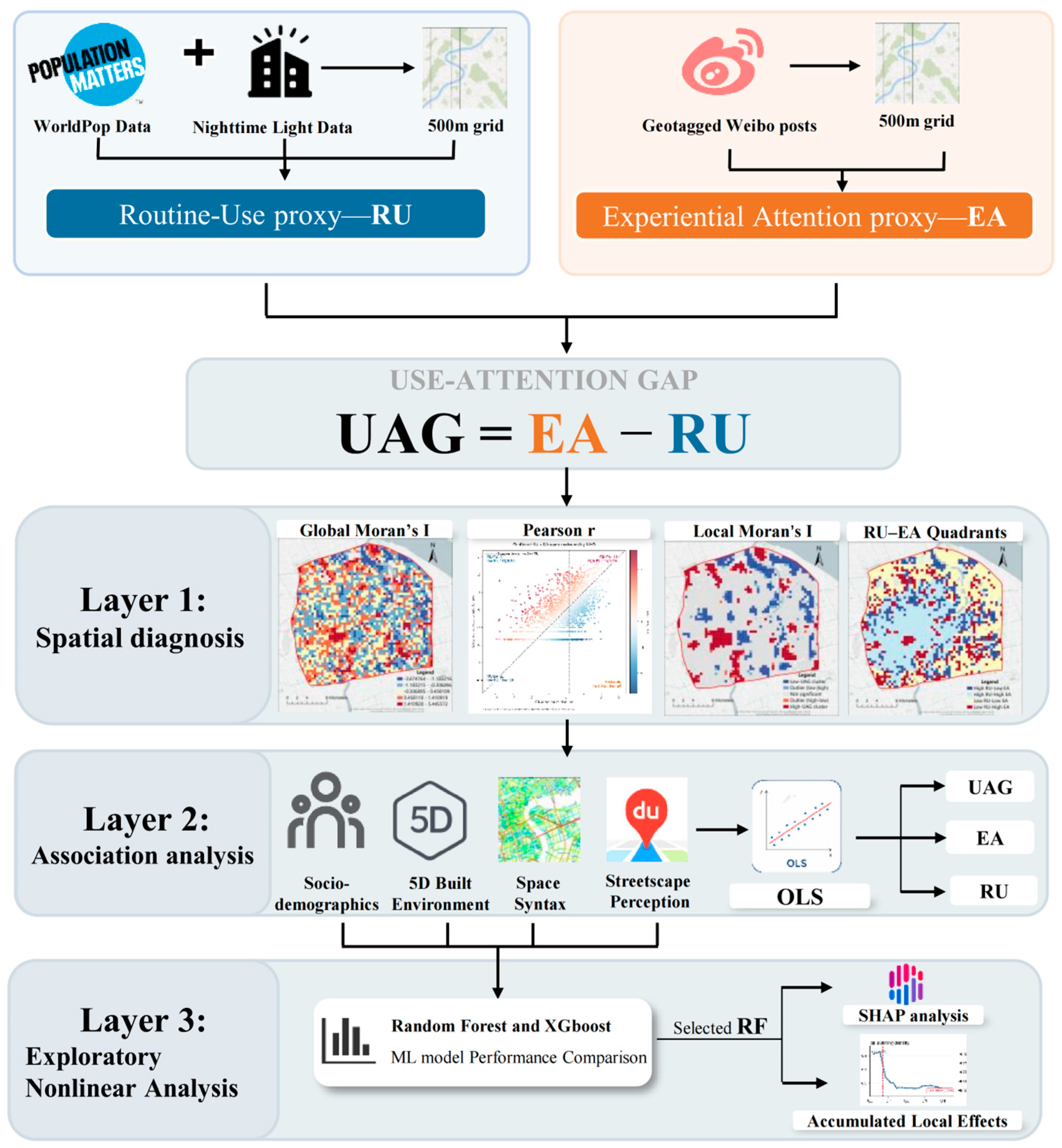
Conceptually, the Use–Attention framework distinguishes recurrent functional engagement from digitally expressed experiential attention. This conceptual distinction may be applied in other urban contexts, but the numerical UAG analyzed here is a case-specific operationalization based on WorldPop, VIIRS, and Weibo data at 500 m resolution in central Shanghai; it is not a universally fixed metric. The analysis proceeds in five steps (Figure 1). First, two grid-level proxy indicators are constructed: RU combines gridded population and nighttime-light intensity to approximate recurrent functional occupation [34,35], whereas EA is derived from geotagged Weibo posts to approximate where place-based experiences are deliberately made visible through digital posting [5,7,21]. Second, both proxies are z-standardized and the case-specific UAG indicator is computed as EA − RU. Third, global and bivariate Moran’s I, grid-level Pearson correlation, median-split quadrant classification, and LISA assess whether the proxy dimensions and their relative contrast are spatially aligned or systematically divergent. Fourth, UAG is modeled against socio-demographic characteristics, 5D indicators, space-syntax configuration measures, and streetscape perception indicators through standalone, hierarchical, and full Ordinary Least Squares (OLS) specifications; the same full model is estimated with RU and EA as dependent variables to identify which proxy dimension underlies each UAG association. Finally, Random Forest and XGBoost models, implemented using scikit-learn (version 1.5.1) and the xgboost package (version 3.2.0), respectively, are combined with SHAP and ALE to examine exploratory nonlinear predictive patterns across RU, EA, and UAG.

2.2. Study Area and Analytical Unit

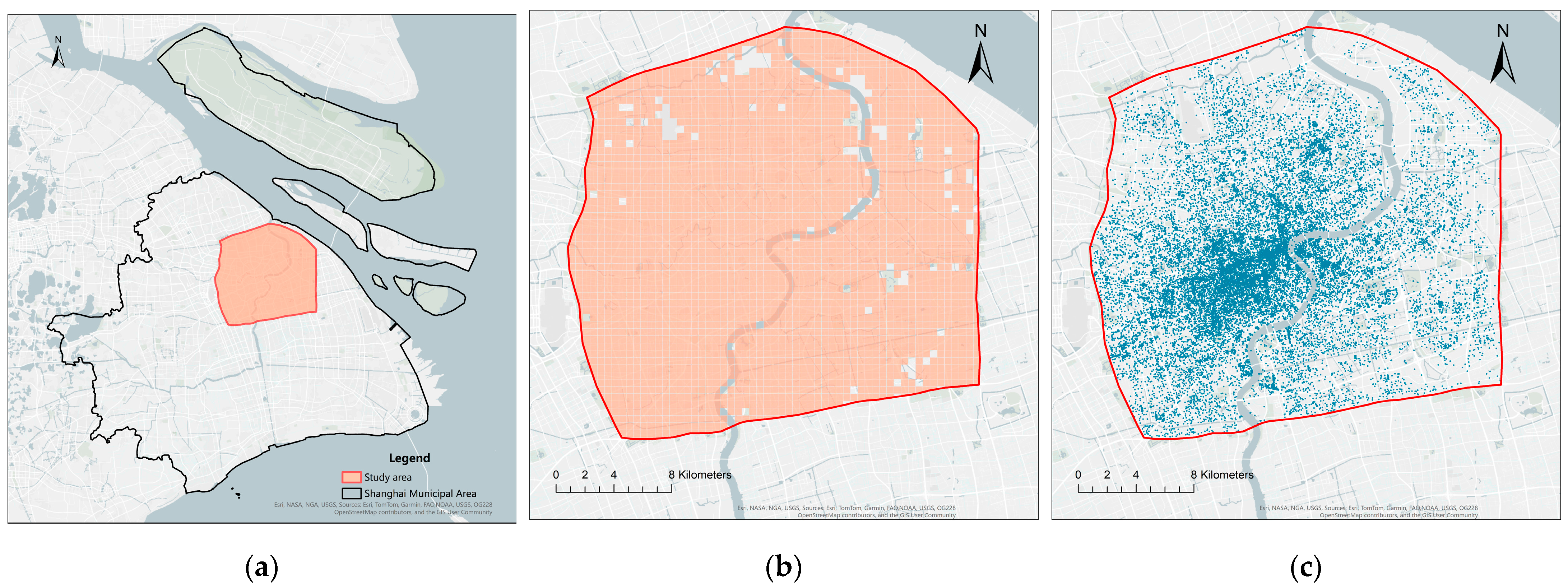
The study area covers the region within the Outer Ring Expressway in central Shanghai, approximately 620 km² (Figure 2). It encompasses core Puxi districts (Huangpu, Jing’an, Xuhui, Changning, Hongkou, and Yangpu) and the inner-ring portion of Pudong New Area. The area contains the highest population density and the greatest functional diversity in the Shanghai metropolitan region [20,33]. The study area includes historic lane-house neighborhoods, waterfront promenades, large residential estates, commercial corridors, and inner-suburban activity nodes.

We adopt a 500 m × 500 m regular grid as the analytical unit, following neighborhood vitality studies at the same resolution [19,29]. This cell size approximates a short walking catchment and provides a common neighborhood-scale unit for aggregating geotagged Weibo posts and Point of Interest (POI) data. After excluding cells that lack valid streetscape perception scores or space-syntax configuration measures, 2615 of the initial 2769 grids remain. Figure 2 shows the study area and analytical grid alongside the distribution of geotagged Weibo posts.

2.3. Construction of Routine Use, Experiential Attention, and the Use–Attention Gap

Because recurrent functional use and digitally expressed experiential attention are latent dimensions that cannot be exhaustively observed through a single dataset [9,10], RU and EA are operationalized as theoretically informed proxy indicators derived from distinct observable manifestations of spatial engagement. RU approximates recurrent human presence and infrastructure-supported urban functioning, whereas EA approximates the deliberate, platform-mediated visibility of place-based experiences. The case-specific UAG indicator is then calculated as the difference between these standardized proxy measures.

Routine-use intensity (RU) combines WorldPop 2024 gridded population (≈100 m raster, zonal sum) and VIIRS 2024 nighttime-light intensity (≈500 m raster, NOAA, zonal mean). WorldPop provides fine-scale, spatially explicit estimates of resident population, including validated high-resolution population distributions for the Chinese context [36,37]. In this study, it represents the relatively stable resident base from which repeated household activities, daily departures and returns, and recurring demand for neighborhood services are generated. VIIRS directly observes artificial low-light emissions, and prior studies show that nighttime radiance is systematically associated with human settlements and with local demographic, socioeconomic, and infrastructure conditions [38,39]. Residential lighting, office operations, retail and service provision, transport facilities, and evening leisure activities all contribute to this electricity-dependent signal [38]. Nighttime light is therefore interpreted as an aggregate indication of sustained electrified urban operation rather than as a direct count of people, trips, or visits. Combining the resident population base with nighttime radiance broadens the observable content of RU beyond either source alone. Nevertheless, the composite may also capture general urban intensity and does not directly observe commuting purposes, transient daytime populations, pedestrian movement, or all forms of everyday use [37,38,39]. RU is consequently interpreted as an indicative proxy for recurrent functional occupation rather than as a complete measure of routine behavior or mobility. Both inputs are log1p-transformed and z-standardized before being averaged with equal weights:

$${\widetilde{\mathrm{R}\mathrm{U}}}_{\mathrm{i}}=\left[\mathrm{z}\left(\log 1\mathrm{p}\left({\mathrm{p}\mathrm{o}\mathrm{p}\_\mathrm{s}\mathrm{u}\mathrm{m}}_{\mathrm{i}}\right)\right)+\mathrm{z}\left(\log 1\mathrm{p}\left({\mathrm{n}\mathrm{t}\mathrm{l}\_\mathrm{m}\mathrm{e}\mathrm{a}\mathrm{n}}_{\mathrm{i}}\right)\right)\right]/\hspace{0.17em}2$$

(1)

The intermediate composite is z-standardized to give the final RU score:

$${RU}_i=z\left({\widetilde{RU}}_i\right)$$

(2)

Equal weights are used because population and nighttime light represent complementary manifestations of recurrent functional occupation: the stable resident base that repeatedly generates activity demand and the sustained electricity-dependent operation of urban functions. Results are robust to weights ranging from 0.3/0.7 to 0.7/0.3 (Table S1).

Digitally expressed experiential-attention intensity (EA) is constructed from geotagged Weibo posts. Previous urban studies have used geotagged social-media data to characterize one dimension of urban vibrancy and dynamics, reveal mobility and preference patterns, and approximate the popularity of places [7,9,22,40]. The relevance of these records to EA lies in their data-generating process: a user actively associates a public post with a geographic location, thereby converting a place-based experience into a digitally visible and communicable trace [21,22]. Aggregated records therefore indicate where places are more frequently selected for public digital expression. They do not measure total visitation, the full range of experiential attention, or the preferences of the entire population.

EA is calculated from public Sina Weibo posts with user-attached geographic coordinates rather than venue transactions linked to specific establishments [9,40]. The records span the full year 2024 and were collected from the Sina Weibo open platform (https://open.weibo.com). W_i denotes the raw geotagged-post count within grid i; because the dataset does not include user-level identifiers, W_i is an aggregate intensity measure and does not represent a unique-visitor count. The geographic coordinates were used solely to assign the posts to 500 m grid cells, and no user-level identifiers were retained in the analytical dataset. Records lacking valid coordinates or falling outside the study-area boundary are removed before spatial joining to the 500 m grid; 885,039 records fall within the 2615 valid grids (2255 grids with at least one record, 360 with none). Zero-count grids are retained because the absence of a recorded post is a meaningful value of the EA proxy rather than missing data. A 0.5 offset keeps these grids on a finite scale after log-transformation, and EA is defined as:

$${EA}_{\mathrm{i}}=z\left[log\left(W_{\mathrm{i}}+0.5\right)\right]$$

(3)

The distinction between RU and EA is grounded in the different mechanisms through which the observable traces are generated. RU-related signals arise from persistent residential concentration and repeated urban operation regardless of whether activities are publicly recorded. EA-related signals become observable when users deliberately associate public digital content with places. The former therefore approximates recurrent functional occupation, whereas the latter approximates digitally expressed place salience. Neither proxy exhaustively measures its corresponding construct, but each records a theoretically relevant manifestation of a different mode of spatial engagement.

Because RU and EA are each z-standardized, the case-specific UAG indicator is calculated as their direct difference:

$${UAG}_{\mathrm{i}}={EA}_{\mathrm{i}}-{RU}_{\mathrm{i}}$$

(4)

Positive UAG values indicate that the standardized EA proxy is higher than the standardized RU proxy within the study sample, whereas negative values indicate that the RU proxy is relatively higher. Values near zero indicate similar standardized proxy scores. These contrasts do not establish absolute experiential dominance, inadequate public or planning attention, or equality between the underlying behaviors; they describe only the relative position of two case-specific proxies.

UAG is not z-standardized again after subtraction. Retaining the direct difference preserves its interpretation in the common standardized units of the two proxy indicators. Its numerical values are sample-relative and conditional on the selected data sources, transformations, 500 m spatial unit, study period, and Shanghai context.

As a scaling sensitivity check, RU and EA are also transformed using empirical-rank inverse-normal scores. Tied values, including zero-post-count grids, receive the same average rank. The alternative gap is defined as UAG_rank = EA_rank − RU_rank. This specification reduces sensitivity to the zero offset and extreme values while preserving the ordinal geography of both indicators (Table S9).

2.4. Spatial Diagnosis of Use–Attention Gap

We calculated global Moran’s I separately for RU, EA, and UAG to assess the degree of spatial clustering in each measure [41]. All spatial statistics in this section use a row-standardized eight-nearest-neighbor weights matrix (999 random permutations).

Pearson’s r across the 2615 grids quantifies the grid-level correspondence between RU and EA. Bivariate Moran’s I extends the comparison to neighboring grids by measuring the spatial correlation between one indicator at a given grid and the other at adjacent grids [42,43]. The local indicator is calculated as:

$$I_i^{kl}=z_{i,k}\sum _j{w}_{ij}{z}_{j,l}$$

(5)

where $z_{i,k}$ and $z_{j,l}$ are the standardized values of RU at grid i and EA at neighboring grid j, and $w_{ij}$ is the spatial weight. An RU–EA scatter plot colored by UAG visualizes departures from the 45-degree line.

Following Xu et al. [20], we cross-classified grids by the medians of RU and EA, yielding four types: High RU–High EA, High RU–Low EA, Low RU–High EA, and Low RU–Low EA. A grid classified as Low RU–High EA, for example, has routine-use intensity below the median and experiential attention intensity above it. The continuous UAG value is retained alongside the typology as the gap intensity entered into subsequent models.

We calculated Local Moran’s I for UAG to identify grids where positive or negative gap values concentrate spatially. This statistic detects whether a grid and its neighbors share similarly high or low UAG values and locates contiguous gap clusters. In the LISA results, high–high and low–low clusters denote local associations in UAG values, not the four RU–EA types defined above. UAG high–high clusters indicate neighboring grids with relatively higher standardized EA proxy scores than RU proxy scores, whereas low–low clusters indicate the reverse. We cross-tabulated the LISA-classified grids with the four RU–EA types to examine whether gap concentrations coincide with particular combinations of RU and EA. All global and bivariate Moran’s I values are re-estimated under k = 4 and k = 6 nearest-neighbor weights; results are directionally consistent across the three specifications (Table S2).

2.5. Explanatory Variables and Data Alignment

The explanatory variables are organized into four groups: 5D indicators, space-syntax configuration measures, streetscape perception indicators, and socio-demographic characteristics (

Table 1. Explanatory variables and theoretical roles.

Group	Variable	Definition	Data Source (Year)
5D indicators	Building density	Building footprint area ratio within grid	Baidu Footprints (2024)
	POI functional mix	Shannon entropy over POI major categories within grid (Diversity—functional mix).	Amap (Gaode) POI (2024)
	Intersection density	log(1 + number of intersections) within grid.	OSM (2024)
	Road density	Road-length density within grid (Design).	OSM (2024)
	Road connectivity	Road network connectivity within grid.	OSM (2024)
	Service accessibility	Min-max normalized count of service POIs within 500 m buffer; log(1 + x), z-standardized.	Amap (Gaode) POI (2024)
	Distance to center	Distance from grid centroid to nearest metropolitan center (km).	Amap (2024)
	Distance to metro	log(1 + distance to nearest metro station) (Distance to transit).	Amap (2024)
	Bus-stop density	log(1 + bus-stop density) within grid (Distance to transit).	Amap (2024)
Space-syntax configuration measures	Syntactic integration	Syntactic integration of road segments aggregated to grid (DepthMapX).	OSM + DepthMapX (2024)
	Space-syntax connectivity	Space-syntax connectivity of road segments aggregated to grid.	OSM + DepthMapX (2024)
Streetscape perception indicators	Streetscape PC1	First principal component of six MIT-style perception scores; a general positive-perception component (higher safety, beauty, liveliness, and wealth; lower boredom and depression).	Baidu Street View imagery; MIT Place Pulse-style perception scoring pipeline
	Streetscape PC2	Second principal component of the same six perception scores; an aesthetic–quiet component contrasting visually pleasant, calmer streetscapes with more lively ones.	Baidu Street View imagery; MIT Place Pulse-style perception scoring pipeline
Socio-demographic characteristics	Working-age population	Share of population aged 15–59; area-weighted to grid.	7th Census (2020)
	Education percentile rank	Zonal mean of the 2020 education percentile rank GeoTIFF.	Zhang et al. (2026), community-level education percentile rank GeoTIFF, 2020.

Note: $pop\_sum$ and $ntl\_mean$ are used to construct ${\widetilde{RU}}_i$, which is standardized again as ${RU}_i$; $wb\_count$ is used to construct ${EA}_{\mathrm{i}}$. UAG is defined as ${EA}_{\mathrm{i}}-{RU}_i$. The remaining variables are predictors in the UAG models.

).

The 5D indicators and socio-demographic characteristics are defined in Table 1. POIs are obtained from the Amap data and reclassified from the Amap first-level category into six functional classes: commercial retail, dining, business and office, public services, recreation and leisure, and transport facilities. Functional mix is calculated as Shannon entropy across these six classes within each grid, with the mapping from Amap first-level categories to the six functional classes reported in Table S3. Educational composition is measured as the grid-level zonal mean of the 2020 mean education percentile rank raster developed by Zhang et al. [44]. Working-age population share is derived from the Seventh National Population Census (2020) [45] and matched to the 500 m grid through area-weighted allocation; it and distance to metro enter the models as controls to absorb demographic and transit-proximity effects.

Because accessibility and network position shape how people encounter and move through urban space, this study incorporates space-syntax measures to capture the configurational advantages of different locations. Space-syntax configuration measures describe the movement potential that the street network affords to each location [46,47]. Syntactic integration indexes how easily a road segment can be reached from the rest of the network, and space-syntax connectivity records how many segments directly connect to it. Both are computed from the OSM road network at global radius (Rn) using angular segment analysis in DepthMapX (version 0.8.0) and aggregated to each 500 m grid as segment-length-weighted means; because the network is clipped at the study-area boundary, integration values in edge grids may be attenuated.

Beyond structural accessibility, the visual qualities of streets also shape how urban spaces are experienced and attended to, so this study includes streetscape perception indicators to represent the human-scale environment. Streetscape perception indicators capture the human-scale visual environment from street-view imagery [48,49]. Baidu Street View images acquired in 2024 are sampled at 50 m intervals along road centerlines, yielding 72,552 valid sample points. Each image is scored on six perceptual dimensions (safety, liveliness, beauty, wealth, boredom, and depression) using a multi-task DenseNet-121 model pretrained on the Place Pulse 2.0 dataset [49,50]. The use of this model in Shanghai is intended as a transfer-learning application rather than a claim of direct cultural equivalence between the original training context and the present study area. Its use is supported by two considerations. First, the six perception dimensions are broad visual judgments that have been widely used in comparative streetscape research. Second, closely related Place Pulse–style models have been applied in prior studies using Chinese street-view imagery, suggesting that the learned visual features retain practical descriptive value in this context [29,50]. At the same time, the scores should be interpreted as model-based proxies of relative visual perception rather than direct measurements of how all local residents evaluate streetscapes in Shanghai. This limitation is revisited in Section 4.5. Point-level scores are averaged within each 500 m grid; grids without valid sample points are excluded from the analysis. The six grid-level scores are reduced to two principal components before modeling. PC1 loads positively on safety, beauty, liveliness, and wealth and negatively on boredom and depression, and is therefore interpreted as a general positive-perception component. PC2 captures a contrast between aesthetically pleasant, quieter streetscapes and more animated ones: in substantive terms, it distinguishes visually appealing but relatively calm environments from streetscapes more strongly associated with liveliness. For ease of interpretation, PC2 is labeled the aesthetic–quiet component. Loadings and explained-variance ratios for both components are reported in Supplementary Table S4.

Before entering the models, skewed non-negative predictors are log1p-transformed as indicated in Table 1. The initial predictor pool contains 16 variables. Collinearity among the predictor set is screened with variance inflation factors: POI density is removed because of collinearity with service accessibility, and the 15 retained predictors all have VIF values below 3. Descriptive statistics and VIF values for RU, EA, UAG, and the 15 predictors are reported in Table S5.

2.6. Spatial Regression Models (OLS and Spatial Error Model)

All continuous predictors are z-standardized before entry. UAG itself is not re-standardized after subtraction. We fitted socio-demographic characteristics, 5D indicators, space-syntax configuration measures, and streetscape perception indicators to UAG cumulatively in the order listed (Table S6); the full model enters all groups simultaneously:

$$\begin{gathered} {\mathrm{U}\mathrm{A}\mathrm{G}}_{\mathrm{i}}={\mathsf{\beta }}^0+{\mathrm{X}}_{\mathrm{d}\mathrm{e}\mathrm{m}\mathrm{o},\mathrm{i}}{\mathsf{\beta }}_{\mathrm{d}\mathrm{e}\mathrm{m}\mathrm{o}}+{\mathrm{X}}_{5\mathrm{D},\mathrm{i}}{\mathsf{\beta }}_{5\mathrm{D}} + \\ {\mathrm{X}\_\mathrm{s}\mathrm{y}\mathrm{n}\mathrm{t}\mathrm{a}\mathrm{x},}_{\mathrm{i}}\mathsf{\beta }\_\mathrm{s}\mathrm{y}\mathrm{n}\mathrm{t}\mathrm{a}\mathrm{x}+{\mathrm{X}\_\mathrm{s}\mathrm{t}\mathrm{r}\mathrm{e}\mathrm{e}\mathrm{t},}_{\mathrm{i}}\mathsf{\beta }\_\mathrm{s}\mathrm{t}\mathrm{r}\mathrm{e}\mathrm{e}\mathrm{t}+{\mathsf{\epsilon }}_{\mathrm{i}}. \end{gathered}$$

(6)

Significance tests for all OLS coefficients use HC3 heteroscedasticity-consistent standard errors. The same specification is estimated with RU and EA as dependent variables, so that each predictor’s association with the gap can be traced to routine use, experiential attention, or both. To account for spatial dependence, we compute residual Moran’s I and robust Lagrange Multiplier diagnostics on the row-standardized eight-nearest-neighbor weight matrix and estimate a spatial error model alongside OLS:

$${\mathrm{U}\mathrm{A}\mathrm{G}}_{\mathrm{i}}={\mathrm{X}}_{\mathrm{i}}\mathsf{\beta }+{\mathrm{u}}_{\mathrm{i}}, {\mathrm{u}}_{\mathrm{i}}=\mathsf{\lambda }{\mathsf{\Sigma }}_{\mathrm{j}}{\mathrm{w}}_{\mathrm{ij}}{\mathrm{u}}_{\mathrm{j}}+{\mathsf{\epsilon }}_{\mathrm{i}}.$$

(7)

where X_i is the full predictor vector, w_ij the spatial weights, and λ the spatial autocorrelation coefficient. Associations whose direction and significance remain stable across the two specifications are considered robust to residual spatial dependence. The spatial error model is re-estimated under k = 4 and k = 6 weights; λ remains significant and most coefficient signs are unchanged, with exceptions noted in Table S7.

2.7. Tree-Based Models and Interpretation (Random Forest, XGBoost, SHAP, and ALE)

The linear assumption underlying OLS cannot capture the nonlinear associations that are likely to shape RU, EA, and UAG. Building upon the full OLS specification, the analysis therefore advances into machine-learning algorithms. Random Forest and XGBoost are fitted to all three outcomes using the same predictor set, as both algorithms are adept at modeling nonlinear and interaction effects while offering clear interpretation in urban research. Both models are tuned via grid search with five-fold cross-validation. The optimal Random Forest configuration uses 300 trees, a minimum leaf size of 5, and 80% feature sampling per split. The optimal XGBoost configuration uses 350 trees with a maximum depth of 3, a learning rate of 0.04, row and column subsampling of 85%, and an L2 penalty (reg_lambda) of 5.0. ALE profiles are computed over a maximum of 20 quantile-based bins. The 2615 grids are partitioned into training (70%), validation (15%), and test (15%) sets with the same split applied to all three outcomes, and the best-performing model family on the validation set is carried forward to reveal the nonlinear structure of UAG. A buffered spatial block cross-validation (5 km blocks, adjacent blocks excluded from training) is conducted to check for spatial leakage in the random partition [51] (Table S8).

The fitted models are interpreted with TreeSHAP [52] for variable importance and ALE plots [53] for response shapes. ALE is preferred to partial dependence because it is less sensitive to correlated predictors, a relevant consideration given the collinearity among built-environment variables in these data. SHAP values are aggregated within the four predictor groups to reveal which dimensions of the built environment weigh more heavily on the gap than on either indicator alone. ALE curves trace how predicted UAG changes across the range of each predictor, identifying the built-environment conditions under which the gap shifts direction or intensifies. Tree-based models are used exploratorily to characterize within-sample nonlinear structure in the observed Shanghai sample. Because spatially buffered validation provides a more conservative test of geographic transferability, SHAP importance and ALE profiles are interpreted as descriptions of the fitted models rather than as causal effects, transferable prediction rules, or planning thresholds.

3. Results

3.1. Spatial Distribution of RU, EA, and UAG

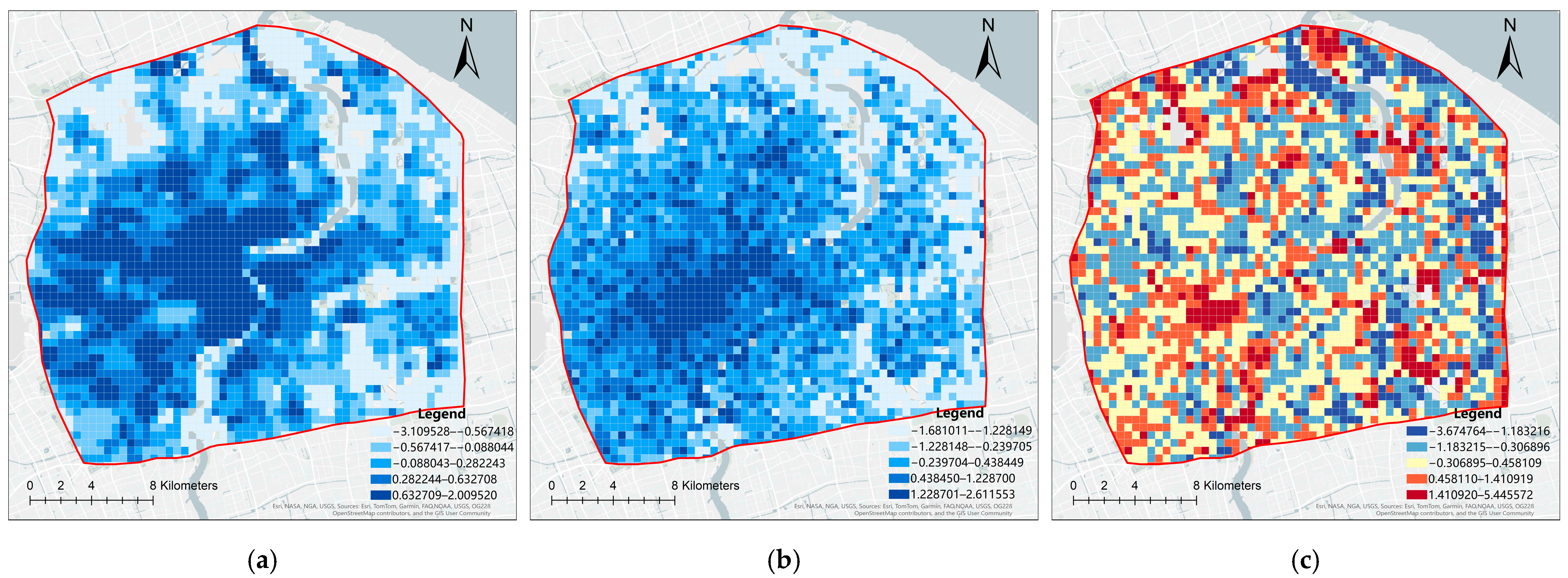
Figure 3 maps the spatial distributions of routine use (a) and experiential attention (b), which differ in degree of spatial autocorrelation and in spatial pattern. Routine use exhibits strong positive spatial autocorrelation (Moran’s I = 0.752, p < 0.001,

Table 2. Descriptive statistics and global Moran’s I of RU, EA, and UAG.

Variable	Moran’s I	Moran z	p
RU	0.752	77.819	<0.001
EA	0.635	65.731	<0.001
UAG	0.417	43.204	<0.001

) and grades from a continuous high-value core in central Puxi (Nanjing East Road–Bund, Nanjing West Road–Jing’an, Huaihai Road–Xintiandi) through the Lujiazui–Century Avenue corridor to low values at the Baoshan and outer-Pudong industrial–logistics fringe (Figure 3a). Spatial autocorrelation is weaker but significant for experiential attention (Moran’s I = 0.635, p < 0.001; Figure 3b). High experiential-attention values align with commercial corridors and heritage areas, concentrated along the central Puxi commercial spine (Nanjing East Road–Bund, Huaihai Road–Xintiandi) and the Hengfu/Wukang historical district in Xuhui, with a secondary concentration at Lujiazui–Tangqiao in Pudong. The residential interior and the industrial–logistics fringe remain low for both measures.

At the grid level, RU and EA are only moderately correlated (Pearson r = 0.490; Figure S1): less than a quarter of the variance in either indicator is shared with the other.

UAG shows moderate positive spatial autocorrelation (Moran’s I = 0.417, p < 0.001; Figure 3c). Positive-UAG grids, where the standardized EA proxy is relatively higher than the RU proxy, form continuous bands along waterfront and heritage corridors, concentrated around the Hengfu/Wukang historic quarter, the Expo–Qiantan waterfront, and several consumption subcenters in Pudong. Negative-UAG grids, where the standardized RU proxy is relatively higher, spread across the northern and eastern industrial margins of Pudong and the Yangpu–Baoshan belt. These patterns describe spatial contrasts between proxies rather than absolute experiential or routine-use dominance.

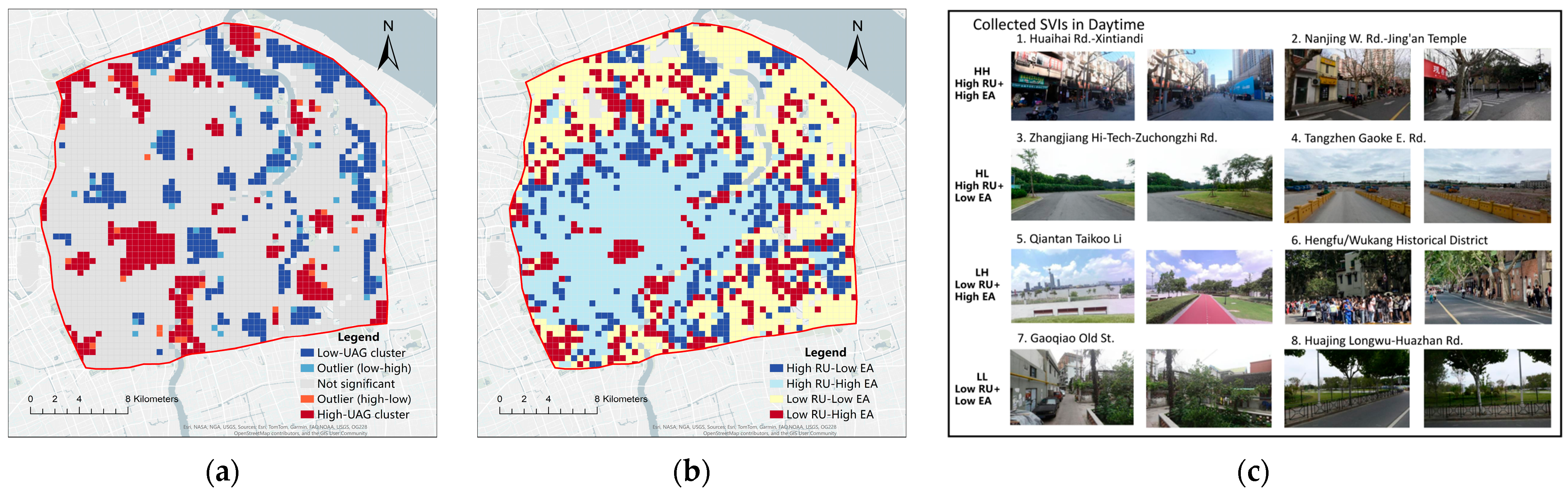
The median-split cross-classification of RU and EA yields four quadrant types (Figure 4b). High RU–High EA (n = 903, 34.5%) and Low RU–Low EA (n = 900, 34.4%) together account for nearly 70% of all grids. High RU–High EA forms a continuous zone extending across the Puxi inner city into the Lujiazui–Century Avenue corridor. Low RU–Low EA occupies a broad peripheral belt spanning northern and eastern Pudong and the Baoshan–Yangpu margin, with extensions into selected southern corridors. High RU–Low EA grids (n = 405, 15.5%) appear as pockets along the northern industrial fringe and in eastern Pudong. Low RU–High EA grids (n = 407, 15.6%) concentrate at commercial and waterfront nodes, including Beicai–Zhangjiang and the Expo waterfront–Shanggang corridor, with additional occurrences near the Pengpu–Miaohang interface.

3.2. Spatial Clustering of UAG

Local Moran’s I identifies 319 high-UAG and 372 low-UAG cluster grids, together covering 26.4% of all grids (

Table 3. UAG LISA categories by RU–EA quadrant type.

LISA Cluster	High RU– High EA	High RU– Low EA	Low RU– High EA	Low RU– Low EA	Total n	Share of All Grids
High-UAG cluster	59 (18.5%)	0 (0.0%)	124 (38.9%)	136 (42.6%)	319	12.2%
Spatial outlier	27 (37.5%)	0 (0.0%)	15 (20.8%)	30 (41.7%)	72	2.8%
Low-UAG cluster	75 (20.2%)	154 (41.4%)	0 (0.0%)	143 (38.4%)	372	14.2%
Not significant	742 (40.1%)	251 (13.6%)	268 (14.5%)	591 (31.9%)	1852	70.8%
Total	903 (34.5%)	405 (15.5%)	407 (15.6%)	900 (34.4%)	2615	100.0%

Note: Each cell shows n (row %). Columns follow the median-split RU–EA typology and rows follow local Moran’s I on UAG; outliers are grids whose UAG differs significantly from that of their neighbors. High-UAG clusters contain neighboring grids with relatively higher standardized EA proxy scores than RU proxy scores, whereas low-UAG clusters contain neighboring grids with relatively higher RU proxy scores. These labels describe relative proxy contrasts and should not be interpreted as absolute behavioral dominance.

; Figure 4a). High-UAG clusters fall predominantly in Low RU–Low EA and Low RU–High EA grids, and low-UAG clusters in High RU–Low EA and Low RU–Low EA grids. Within the Low RU–Low EA belt, High-UAG clusters scatter across northern Baoshan and the Shanggang–Qiantan waterfront fringe. Along the industrial and port margins of eastern Pudong and the northern Yangpu–Baoshan fringe, Low-UAG clusters predominate. The High RU–High EA core also contains both cluster types: 59 of the 319 High-UAG cluster grids (18.5%) and 75 of the 372 Low-UAG cluster grids (20.2%) fall within this zone (Table 3). Spatial outliers are few (72 grids, 2.8%), and the gap pattern consists mainly of contiguous clusters.

3.3. Regression Analysis of the Use–Attention Gap

Section 3.2 established that UAG is spatially clustered.

Table 4. OLS and spatial error model coefficients for RU, EA, and UAG.

Group	Variable	RU OLS β	EA OLS β	UAG OLS b	UAG SEM b (k = 8)
5D	Building density	+0.159 ***	−0.015	−0.174 ***	−0.166 ***
5D	POI functional mix	+0.226 ***	+0.105 ***	−0.121 ***	−0.093 ***
5D	Road connectivity	−0.004	−0.087 ***	−0.083 ***	−0.050 *
5D	Distance to metro (log)	−0.101 ***	−0.001	+0.100 ***	+0.045 *
5D	Service accessibility (log)	+0.183 ***	+0.262 ***	+0.079 **	−0.099 **
Demographic	Working-age pop. share	−0.037 **	−0.174 ***	−0.138 ***	−0.030
Spatial syntax	Syntactic integration	+0.124 ***	+0.210 ***	+0.086 ***	+0.061
Streetscape	Streetscape PC2	−0.108 ***	−0.012	+0.096 ***	+0.048 *
5D	Intersection density (log)	+0.131 ***	+0.118 ***	−0.013	−0.026
5D	Road density	+0.072 ***	+0.084 ***	0.012	−0.021
5D	Distance to center	−0.080 ***	−0.064 ***	0.016	−0.002
5D	Bus-stop density (log)	−0.007	−0.023	−0.016	−0.021
Demographic	Educational attainment	+0.065 ***	+0.091 ***	0.026	−0.003
Spatial syntax	Space-syntax connectivity	0.024	−0.014	−0.037	−0.003
Streetscape	Streetscape PC1	+0.064 ***	+0.039 *	−0.025	−0.060 **
Spatial diagnostic	Spatial-error coefficient λ	—	—	—	+0.786 ***
Spatial diagnostic	Residual Moran’s I	—	—	0.396 ***	−0.007

Note: RU and EA columns report HC3-robust OLS estimates. The UAG OLS column also uses HC3-robust standard errors; the UAG SEM column reports the maximum-likelihood spatial error model based on row-standardized k = 8 nearest-neighbor weights. β denotes RU/EA coefficients; UAG coefficients are reported as b. Significance levels are *** p < 0.001, ** p < 0.01, and * p < 0.05. Robust UAG associations retain their direction and significance in both UAG specifications. Residual Moran’s I decreased from 0.396 (p < 0.001) in OLS to −0.007 after spatial-error correction. The three OLS columns in Table 4 should be read jointly. Because UAG is the direct difference between EA and RU, each UAG coefficient represents the net balance of the corresponding EA and RU coefficients rather than an independent third association. Positive UAG coefficients indicate that higher predictor values are associated with a more positive EA–RU proxy contrast, whereas negative coefficients indicate a more negative contrast. The separate RU and EA columns are used to identify which side of the contrast underlies each association.

therefore reports the full UAG OLS model together with the main k = 8 spatial error specification, while the separate RU and EA OLS models identify which side of the gap underlies each association. The hierarchical block results remain in Table S6 and the k = 4, 6, and 8 SEM comparison in Table S7. Because the spatial-error coefficient is large and significant (λ = 0.786, p < 0.001), the interpretation below prioritizes associations that remain stable after spatial correction.

The three OLS columns in Table 4 should be read jointly. Because UAG is the direct difference between the standardized EA and RU proxies, each UAG coefficient represents the net balance of the corresponding EA and RU coefficients rather than an independent third association. Positive values indicate that the corresponding EA coefficient is more positive, or less negative, than the RU coefficient, whereas negative values indicate the reverse. The separate RU and EA columns are therefore used to identify whether the observed UAG association primarily reflects the RU coefficient, the EA coefficient, or both.

Five UAG associations retain both direction and statistical significance across OLS and SEM. Building density remains negatively associated with UAG (OLS b = −0.174; SEM b = −0.166), as do POI functional mix (−0.121; −0.093) and road connectivity (−0.083; −0.050), indicating a more negative EA–RU proxy contrast at higher values of these variables. Distance to the nearest metro station remains positively associated with UAG (+0.100; +0.045), indicating a more positive EA–RU proxy contrast farther from metro stations. Streetscape PC2 also retains a positive association (+0.096; +0.048). These five variables are treated as robust to residual spatial dependence, but the coefficients remain associations with a relative proxy contrast rather than evidence of behavioral dominance.

Several OLS findings are model-sensitive. Syntactic integration is positive and significant in OLS (b = +0.086, p < 0.001) but is no longer significant in the SEM (b = +0.061, p = 0.333). Service accessibility changes from a positive OLS association (b = +0.079, p = 0.003) to a negative SEM association (b = −0.099, p = 0.002). Working-age population share loses significance after spatial correction (−0.138 to −0.030), whereas Streetscape PC1 becomes significant only in the SEM (−0.025 to −0.060). These variables are therefore not interpreted as stable mechanisms of UAG.

The separate RU and EA OLS models remain useful for describing the composition of the two proxy dimensions. For example, service accessibility and syntactic integration are positively associated with the EA proxy in those models. However, these descriptive EA associations do not establish robust positive effects on UAG once residual spatial dependence is addressed. The most defensible UAG interpretation is therefore narrower: higher building density, functional mix, and road connectivity are consistently associated with a more negative EA–RU proxy contrast, whereas greater distance from the nearest metro station and higher values of the aesthetic–quiet streetscape component are associated with a more positive contrast.

This distinction prevents coefficients that are sensitive to spatial specification from being presented as stable planning mechanisms. In particular, service accessibility and syntactic integration may characterize places with higher EA under the OLS decomposition, but their relationship with the gap is contingent on how spatial dependence is modeled.

3.4. Predictability of RU, EA, and UAG Under Tree-Based Models

For UAG, Random Forest is the best-performing model under the random split (test R² = 0.304 vs. 0.131 for OLS;

Table 5. Predictive performance of OLS, Random Forest, and XGBoost for RU, EA, and UAG.

Outcome	Model	Validation R2	Test R2	Test RMSE	Test MAE
RU	OLS	0.636	0.575	0.630	0.474
	Random Forest	0.723	0.695	0.534	0.394
	XGBoost	0.726	0.687	0.541	0.405
EA	OLS	0.400	0.351	0.790	0.618
	Random Forest	0.463	0.492	0.698	0.547
	XGBoost	0.417	0.464	0.718	0.569
UAG	OLS	0.095	0.131	0.975	0.744
	Random Forest	0.197	0.304	0.873	0.679
	XGBoost	0.165	0.282	0.887	0.692

), indicating within-sample nonlinear or interaction-related structure not captured by the linear model; the SHAP and ALE results below are therefore based on it.

Under buffered spatial block validation, Random Forest R² is 0.321 ± 0.171 for RU, −0.117 ± 0.220 for EA, and −0.152 ± 0.151 for UAG (Table S8). The contrast with the random-split results suggests that the random partition partly benefits from local spatial similarity between nearby training and test observations. The negative R² values for EA and UAG indicate performance below a mean-only baseline when predicting spatially separated areas. The tree-based results are therefore interpreted as sample-specific diagnostics of fitted nonlinear patterns rather than as evidence of out-of-area predictive generalization.

3.5. Group-Level Importance

At the group level, the Random Forest SHAP ranking for UAG broadly aligns with the UAG OLS |b|-share ranking, with both placing 5D indicators first (

Table 6. Group-level SHAP importance across RU, EA, and UAG.

Predictor Group	RU Share	EA Share	UAG OLS |b| Share	UAG Share
5D indicators	74.70%	48.80%	60.10%	64.30%
Socio-demographic characteristics	10.10%	30.70%	16.00%	14.60%
Space-syntax configuration measures	10.60%	16.50%	12.00%	13.70%
Streetscape perception indicators	4.60%	4.00%	11.80%	7.50%

). The importance structure shifts across the three outcomes. 5D indicators account for 74.7% of mean |SHAP| for RU but only 48.8% for EA, where socio-demographic characteristics rise from 10.1% to 30.7%. RU appears more closely tied to urban form, and EA more closely tied to population composition. UAG falls between the two (5D 64.3%, socio-demographic 14.6%). Space-syntax and streetscape groups are comparatively stable across all three outcomes.

3.6. Variable Importance and Nonlinear Response Shapes

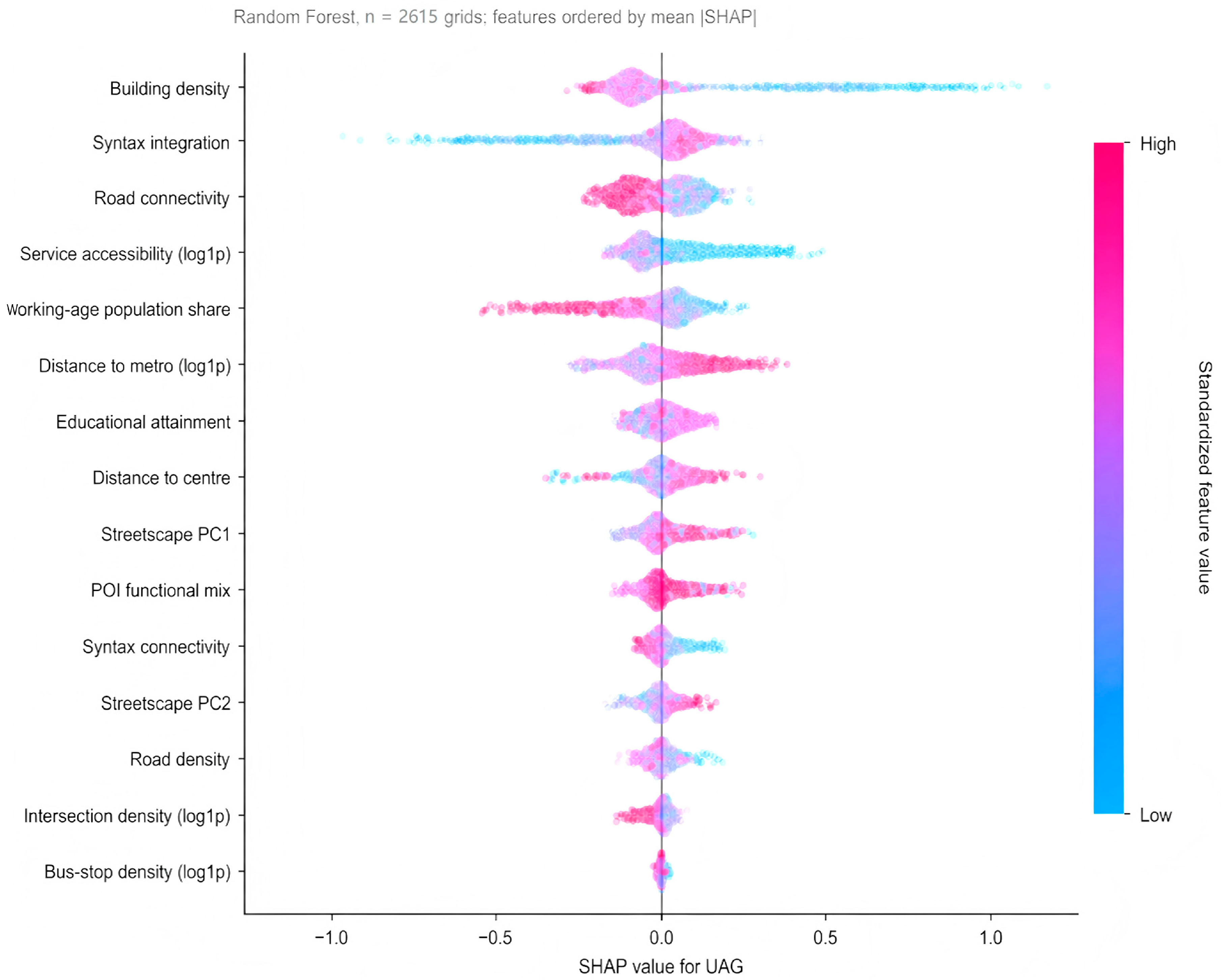
Figure 5 and

Table 7. SHAP-based importance of fifteen predictors for UAG, with group composition.

Factor	Group	Mean |SHAP|	Rel. Importance	Direction	High–Low SHAP
Building density	5D	0.158	20.6%	-	−0.407
Syntactic integration	syntax	0.083	10.7%	+	0.188
Road connectivity	5D	0.080	10.4%	-	−0.180
Service accessibility (log)	5D	0.079	10.3%	-	−0.207
Working-age population share	demo	0.073	9.5%	-	−0.206
Distance to metro (log)	5D	0.066	8.6%	+	0.177
Educational attainment	demo	0.039	5.0%	+	0.029
Distance to center	5D	0.036	4.7%	+	0.061
Streetscape PC1	street	0.035	4.5%	+	0.053
POI functional mix	5D	0.032	4.2%	+	0.051
Syntax connectivity	syntax	0.023	3.0%	-	−0.051
Streetscape PC2	street	0.023	2.9%	+	0.039
Road density	5D	0.021	2.8%	-	−0.040
Intersection density (log)	5D	0.017	2.2%	-	−0.037
Bus-stop density (log)	5D	0.004	0.6%	-	−0.007

Note: Group composition for UAG: G_5D = 64.3% (9 factors; sum mean |SHAP| = 0.495), G_demo = 14.6% (2 factors; 0.112), G_syntax = 13.7% (2 factors; 0.105), and G_streetscape = 7.5% (2 factors; 0.057); total = 0.770. Direction indicates the average SHAP direction for high values of each factor.

report the variable-level Random Forest SHAP results for UAG. Building density is the most important predictor by a clear margin. Syntactic integration, road connectivity, service accessibility, working-age population share, and distance to metro form a second tier of moderate importance, and the remaining nine predictors each contribute little.

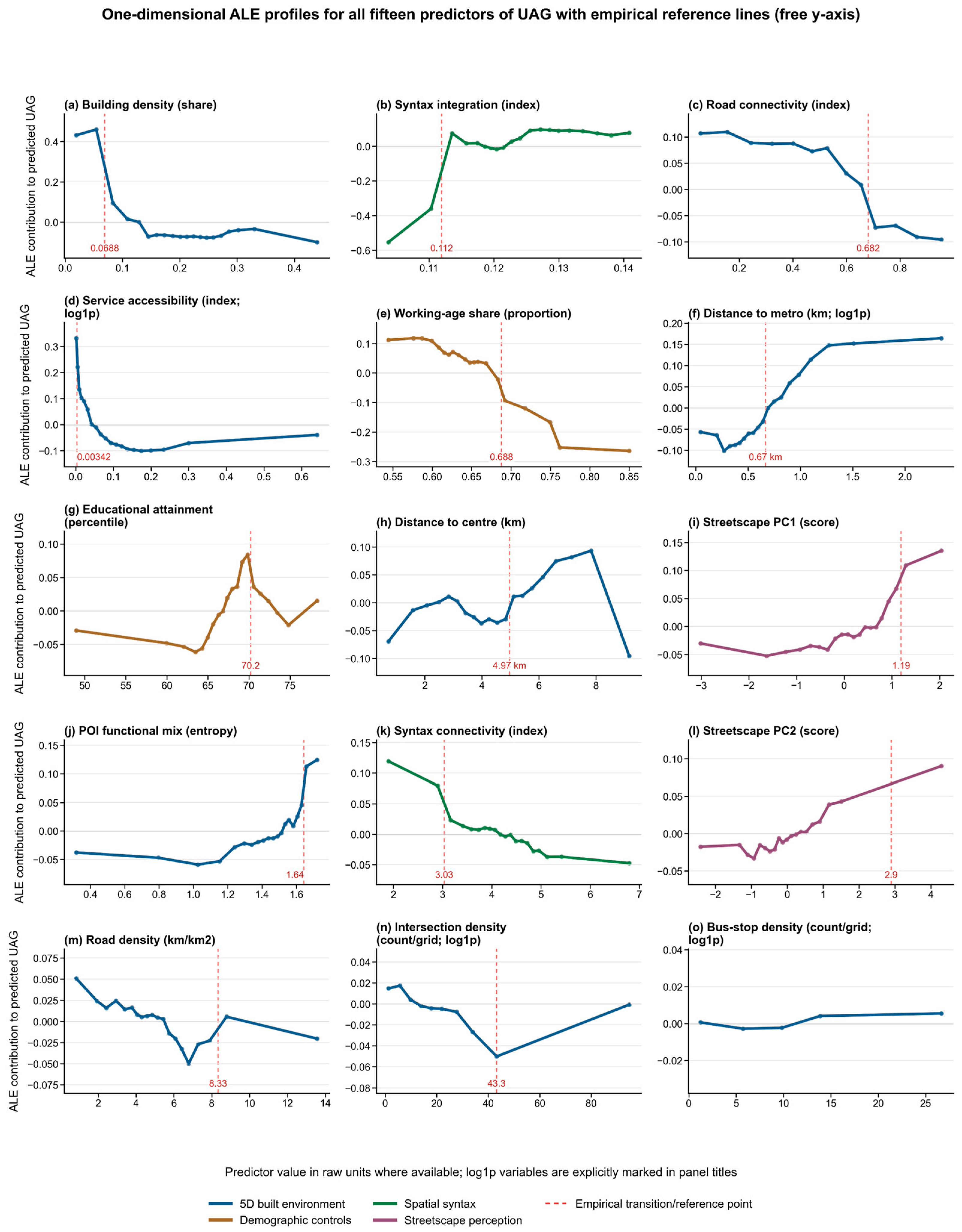
Within the fitted Random Forest model, Figure 6 presents the ALE profiles for all fifteen predictors of UAG and reveals that the relative contrast between the EA and RU proxies is most strongly related to a limited set of variables showing exploratory nonlinear patterns. The strongest pattern is observed for building density, which accounts for 20.6% of mean |SHAP|. Its ALE contribution is highest at very low levels of footprint coverage, then declines sharply once density exceeds approximately 7%, after which the effect remains slightly negative and does not recover. This indicates that higher UAG is most strongly associated with relatively open or weakly built environments rather than with dense residential or mixed-use fabrics. In the study area, such low-density grids are concentrated in waterfront redevelopment zones, open spaces, and areas near major landmarks (Figure 4a), where the standardized EA proxy may be high relative to the RU proxy.

A second set of influential predictors captures the role of street-network structure and locational accessibility. Syntactic integration (10.7%) shows a pronounced transition in the fitted ALE profile: the ALE curve remains nearly flat below a normalized value of about 0.112, rises rapidly within a narrow interval, and stabilizes at a positive plateau between 0.125 and 0.132. The pattern suggests that higher UAG is more commonly associated with places whose network integration exceeds this range. By contrast, distance to metro (8.6%) and distance to center (4.7%) show spatially differentiated and non-monotonic relationships. The contribution of distance to metro shifts from negative near stations to positive beyond roughly 666 m. Because the variable measures distance, this pattern indicates a more positive fitted UAG contribution farther from metro stations, rather than an effect of better metro accessibility. Distance to center becomes positive after about 5 km, peaks near 7.8 km, and declines sharply beyond 9.2 km. Together, these curves indicate that the relative EA–RU proxy contrast is not limited to either central or transit-adjacent areas, but emerges across multiple urban locational contexts.

Several other high-ranking variables show a consistent declining pattern, indicating that UAG becomes weaker as conditions associated with everyday urban functioning intensify. Road connectivity (10.4%) decreases gradually and then more sharply beyond approximately 0.682. Service accessibility (10.3%) has its highest ALE contribution at very low values and levels off as accessibility increases. Working-age population share (9.5%) also becomes negative above about 0.688. Although these variables represent different dimensions of the built and social environment, their response shapes point in the same direction: places characterized by stronger routine mobility, service provision, and resident-based daily activity tend to show lower UAG. This indicates that, within the fitted model, the EA proxy is lower relative to the RU proxy in such settings; it does not establish absolute experiential or routine-use dominance.

The remaining predictors each contribute less than 5% of mean |SHAP|, and their effects are comparatively weak. Within this group, POI functional mix shows a mild positive shift above approximately 1.64, whereas syntax connectivity declines after about 3.03. The other variables do not exhibit clear turning points or stable nonlinear patterns. Overall, the ALE results suggest that UAG is more strongly related to a small number of dominant predictors with turning-point or non-monotonic fitted response shapes. The dashed lines in Figure 6 indicate empirical turning points or transition regions in the fitted ALE profiles. They do not constitute causal thresholds, universal planning standards, or recommended intervention values.

4. Discussion

4.1. Rethinking Urban Space Through Divergent Modes of Spatial Engagement

Multiple findings in this study show that RU (approximated through population grids and nighttime lights) and EA (approximated through geotagged Weibo posts) are not interchangeable indicators of general human activity. Rather, they are theoretically distinct proxy dimensions generated through different observable processes. At the grid level, the two proxies exhibit only a moderate correlation, sharing less than 25% of their variance, and follow different spatial patterns: RU displays a more continuous center-to-periphery gradient, whereas EA is more selectively concentrated around landmarks and commercial corridors. The UAG contrast is itself significantly clustered, indicating a systematic spatial pattern in the relative positions of the two proxies rather than random disagreement between data sources. This evidence supports the conceptual distinction, but it does not convert the proxy scores into complete measurements of the underlying behaviors.

These findings prompt a reconsideration of the prevailing analytical framework through which urban space has traditionally been interpreted [14,54]. While previous multi-source vitality studies have frequently observed “partial overlaps” or mismatches among different data sources, they have traditionally attributed these inconsistencies to inherent data limitations or sampling biases [9,55]. The present analysis interprets such spatial discrepancies as possible manifestations of differing patterns of data generation associated with distinct human motivations.

Consequently, this suggests potential limitations of conventional data-fusion frameworks. Employing homogenizing approaches, such as aggregating these distinct traces of human engagement into a single composite score, may mischaracterize important dimensions of contemporary urban dynamics. Such approaches may distort the interpretation of a series of critical urban indicators, including human activity intensity, urban performance, spatial importance, and overall livability [21,25].

At the same time, the comparison across model families requires a clear distinction between their analytical purposes. OLS summarizes average linear associations, whereas the spatial error model evaluates whether these associations remain stable after residual spatial dependence is accounted for. Random Forest is used to explore nonlinear predictive structure and interactions within the observed sample. Differences in coefficient direction and significance between OLS and the spatial error model, and differences in predictive importance or fitted response shape under Random Forest, therefore represent different forms of evidence and should not be compared as equivalent statistics. Associations that remain stable across OLS and the spatial error model are treated as relatively robust to residual spatial dependence, whereas SHAP rankings and ALE profiles are interpreted as exploratory descriptions of within-sample predictive structure. A high Random Forest importance does not override a loss of significance or sign reversal in the spatial regression results.

4.2. The Spatial Anatomy of Misalignment Between RU and EA

We conceptualize the broader Use–Attention framework as a relational diagnostic lens and the Shanghai UAG as a case-specific support indicator, rather than as a validated decision-making tool or normative evaluative measure. The indicator identifies locations where the two standardized proxy scores differ relatively and may therefore support further investigation of issues such as uneven digital visibility. It does not by itself demonstrate attention bias, planning neglect, experiential dominance, or a need for intervention.

Spatial clustering results indicate a clear geographical differentiation in UAG patterns. Negative-UAG areas, where the RU proxy is relatively higher than the EA proxy, concentrate in Pudong’s industrial zones and the Yangpu–Baoshan corridor. Xu et al. [20] documented that industrial parks and mono-functional residential zones in Shanghai’s suburbs lacked basic public facilities, reducing opportunities for social, economic, and cultural activities. The areas identified here are similarly located, and comparable functional constraints may warrant investigation. Tu et al. [19] further noted that strict functional zoning and large block scales in the Pudong New Area failed to translate spatial investment into positive perceptual outcomes. These comparisons provide contextual hypotheses only: a negative UAG value does not itself establish inadequate services, weak public engagement, or under-attention.

Positive-UAG areas, where the EA proxy is relatively higher than the RU proxy, cluster in the Hengfu historical conservation district and along waterfront zones. Tu et al. [19] documented that historically evolved fine-grained street networks and high visual diversity in Puxi were associated with positive perceptual outcomes. The morphological features of the Hengfu district and waterfront zones may similarly be related to greater digitally expressed place salience relative to the recurrent-use proxy. The prominence of such locations on social-media platforms may also be related to the stronger online engagement often associated with visually distinctive environments [1]. However, a positive UAG value does not demonstrate that experiential activity objectively dominates these places.

Importantly, UAG should not be interpreted through a normative lens of better or worse urban space. For negative-UAG areas, the indicator shows only that the standardized RU proxy is relatively higher than the EA proxy. It does not establish that such places are socially or institutionally under-attended. Where low digital visibility raises a planning question, any response should rely on additional on-site assessment, service audits, investment data, and local consultation rather than on the UAG metric alone [56,57].

For positive-UAG areas, the indicator similarly shows a relative proxy contrast rather than direct evidence of experiential dominance or excessive tourism pressure. It may serve as a signal for closer examination of whether high digital visibility coexists with commercialization, tourism-oriented restructuring, or pressures on residential functions [58,59]. Such interpretations require independent evidence concerning visitation, land-use change, living costs, noise, and local perceptions. UAG alone does not demonstrate that intervention is necessary.

Overall, the Use–Attention framework offers a relational lens for examining whether recurrent functional engagement and digitally expressed attention are spatially aligned. The Shanghai UAG indicator is one case-specific implementation of that framework and should be used as a screening contrast between proxies, not as a direct classification of the underlying urban condition.

4.3. Built-Environment Associations with Routine Use and Experiential Attention

The associations of built-environment characteristics with routine use and experiential attention are not homogeneous. The same feature exhibits varying strengths of association across the two dimensions, with directions that are sometimes consistent and sometimes opposing, thereby revealing an asymmetric pattern of association.

By comparing the OLS coefficients, the separate RU and EA models, and the Random-Forest SHAP results, this study identifies several recurring associations across the non-spatial analyses. Building density (positive association with RU; β = +0.159, 20.6%) and syntactic integration (positive association with EA; β = +0.210, 10.7%) respectively emerge as leading predictors of the two proxy dimensions. However, their implications for UAG are not equally robust after spatial dependence is considered. Building density retains a significant negative association with UAG in both the OLS and spatial error models, whereas the positive OLS association of syntactic integration with UAG becomes non-significant in the spatial error model. Syntactic integration should therefore be interpreted as a factor associated with the EA proxy in the separate outcome model, rather than as a stable correlate of a higher EA-to-RU contrast. POI functional mix and road connectivity retain negative UAG associations after spatial correction, whereas distance to the nearest metro station and Streetscape PC2 retain positive associations. For metro distance, this positive association mainly reflects lower RU farther from stations rather than higher EA. These findings distinguish relative associations with the two proxy dimensions without implying absolute behavioral dominance.

These findings further suggest that density, functional diversity, and street-network connectivity are more consistently associated with the recurrent functional-use proxy. The evidence for conditions associated with relatively higher EA proxy values is more selective and model-dependent. Although syntactic integration and service accessibility are positively associated with UAG in OLS, syntactic integration loses significance and service accessibility reverses sign after spatial correction. By contrast, Streetscape PC2 remains positively associated with UAG across both specifications, suggesting that the aesthetic–quiet streetscape dimension is more consistently related to a higher EA proxy relative to RU. Accordingly, the built environment is associated with differentiated proxy patterns, but the results should not be interpreted as demonstrating that particular factors create attention-dominant or routine-use-dominant spaces.

In addition, the set of built-environment indicators employed in this study engages with the classic Jane Jacobs framework [3] and the traditional “5Ds” paradigm [24,60]. Conventional urban theory often assumes that continuously increasing density and land-use mix are sufficient to automatically generate comprehensive spatial vibrancy. Our results show corresponding positive associations with the RU proxy. They also indicate that, in the context of the digital and attention economy, this foundational relationship requires further qualification: the mere accumulation of physical form is associated with a baseline level of functional urban operation; however, it is not necessarily accompanied by a proportional level of the digitally expressed EA proxy. The spatial-error results do not support treating network integration or service accessibility as stable correlates of a more positive EA–RU proxy contrast. Instead, the more defensible conclusion is that the relationship between the built environment and experiential attention is spatially contingent, with the aesthetic–quiet streetscape dimension providing the most consistent association with a higher EA-to-RU proxy contrast in the present analysis.

4.4. Exploratory Predictability and Nonlinear Patterns in Interpretable Models

This study employs complementary modeling approaches to examine average linear associations, residual spatial dependence, and exploratory nonlinear predictive patterns across RU, EA, and UAG.

Under the random-split evaluation, RU is more predictable from the included built-environment characteristics than EA. However, the substantially lower performance under spatial block validation indicates that this predictive structure partly depends on local spatial similarity. The negative spatial block-validation R² values for EA and UAG show that the fitted models do not generalize reliably to spatially separated areas. The lower within-sample predictability of EA may reflect its stronger association with unobserved socio-cultural dynamics, platform practices, and algorithmic trends beyond the included physical–geographic variables [7].

The ALE profiles provide exploratory descriptions of how fitted predictions vary across the observed predictor ranges. Their turning points may serve as context-specific reference points for interpreting changes in modeled associations within central Shanghai, but they should not be treated as causal breakpoints, universally stable planning thresholds, or fixed intervention targets. Further spatial and external validation would be required before these sample-specific patterns could inform quantitative planning standards [61,62].

4.5. Limitations

Several limitations qualify these findings and indicate directions for further research.

First, both RU and EA are proxy-based measures. RU combines residential population and nighttime-light radiance to indicate recurrent human presence and infrastructure-supported urban functioning, but the composite may also reflect broader urban intensity and does not directly capture all commuting, daytime population redistribution, pedestrian movement, or service use. WorldPop represents a modeled resident population base, while VIIRS radiance may include industrial, road, security, and decorative lighting that is not proportional to contemporaneous human activity [21,38,39]. EA is operationalized through geotagged Weibo posts and therefore captures platform-mediated visibility and digitally expressed place salience rather than experiential attention as a whole [21,22]. Posting behavior is selective with respect to age, platform participation, activity type, and individual propensity to share [21,56]. UAG should consequently be interpreted as a sample-relative contrast between two standardized proxy dimensions, not as the literal difference between all routine use and all experiential behavior or as direct evidence of dominance or neglect. Future research drawing on mobility, pedestrian, survey, investment, or multi-platform data could provide additional triangulation when comparable citywide datasets become available [9,10].

All analyses are conducted at the 500 m grid scale, so UAG represents an aggregated spatial contrast rather than parcel-level or street-segment-level conditions. This aggregation may obscure substantial within-grid variation, especially in mixed-use or morphologically heterogeneous areas. Accordingly, the indicator should not be interpreted as a fine-grained representation of local urban experience.

Second, the study is cross-sectional and therefore identifies associations rather than causal relationships. The built-environment characteristics examined are correlates of the Use–Attention Gap, not established causal determinants of it. The relationship between the physical environment and human behavior is likely reciprocal, with human activity also contributing to changes in the built environment through market forces and policy feedback loops. Longitudinal designs and quasi-experimental approaches would be needed to clarify the direction and stability of these relationships.

Finally, although the conceptual distinction between RU and EA may be applicable beyond Shanghai, the predictive relationships estimated in this study are context-dependent. Urban morphology, functional structure, social-media practices, tourism intensity, and digital participation may alter predictor importance and nonlinear response shapes. The negative spatial block-validation R² values for EA and UAG indicate that the fitted models do not generalize reliably to spatially separated areas within the current study region. Comparative studies across cities and scales are therefore required before the SHAP rankings and ALE patterns can be interpreted as broadly transferable.

5. Conclusions

By integrating multi-source urban data with interpretable machine learning, this study distinguishes recurrent functional use and digitally expressed experiential attention as two theoretically distinct proxy dimensions of urban spatial engagement in central Shanghai. The two proxies are each spatially clustered but follow different geographic patterns and share less than a quarter of their variance at the grid level. Their relative difference forms contiguous spatial clusters, suggesting a systematic spatial pattern in the proxy contrast rather than random variation. The built-environment factors associated with each proxy dimension differ, and the spatial error model identifies which UAG associations remain stable across the selected spatial specifications. Under the random-split evaluation, RU is more predictable than EA, although spatial block validation indicates limited geographic transferability, particularly for EA and UAG. The highest-ranked predictors in the fitted UAG model exhibit exploratory nonlinear response shapes and sample-specific ALE turning points. The broader Use–Attention framework may be adapted to other contexts, but the numerical UAG examined here is a case-specific, sample-relative indicator whose interpretation depends on the selected data sources, transformations, spatial unit, period, and city. It can describe relative contrasts between recurrent functional engagement and digital visibility, but it should not be used to infer absolute experiential dominance, under-attention, or a need for intervention without supplementary evidence.

References

1. Törnberg, P. Social Media Imaginaries and the City: How the Attention Economy Is Reshaping Urban Built Environments. Soc. Media Soc. 2025, 11, 20563051251323389. [Google Scholar] [CrossRef]
2. Cao, L. From online to onsite: Wanghong economy as the new engine driving China’s urban development. Environ. Plan. Econ. Space 2024, 56, 1061–1076. [Google Scholar] [CrossRef]
3. Jacobs, J. The Death and Life of Great American Cities; Random House: New York, NY, USA, 1961. [Google Scholar]
4. Gehl, J.; Koch, J. Life Between Buildings: Using Public Space; Princeton University Press: Princeton, NJ, USA, 2011; ISBN 978-1-59726-827-1. [Google Scholar]
5. Boy, J.D.; Uitermark, J. Reassembling the city through Instagram. Trans. Inst. Br. Geogr. 2017, 42, 612–624. [Google Scholar] [CrossRef]
6. Zou, S. Transcoding a Wanghong City: Mediatized Culturalization of Urban Places in China. Media Cult. Soc. 2025, 47, 22–40. [Google Scholar] [CrossRef]
7. Zhang, F.; Zu, J.; Hu, M.; Zhu, D.; Kang, Y.; Gao, S.; Zhang, Y.; Huang, Z. Uncovering inconspicuous places using social media check-ins and street view images. Comput. Environ. Urban Syst. 2020, 81, 101478. [Google Scholar] [CrossRef]
8. Lynch, K. Good City Form; MIT Press: Cambridge, MA, USA, 1984; ISBN 978-0-262-62046-8. [Google Scholar]
9. Tu, W.; Zhu, T.; Xia, J.; Zhou, Y.; Lai, Y.; Jiang, J.; Li, Q. Portraying the spatial dynamics of urban vibrancy using multisource urban big data. Comput. Environ. Urban Syst. 2020, 80, 101428. [Google Scholar] [CrossRef]
10. Li, X.; Li, Y.; Jia, T.; Zhou, L.; Hijazi, I.H. The six dimensions of built environment on urban vitality: Fusion evidence from multi-source data. Cities 2022, 121, 103482. [Google Scholar] [CrossRef]
11. Montgomery, J. Making a city: Urbanity, vitality and urban design. J. Urban Des. 1998, 3, 93–116. [Google Scholar] [CrossRef]
12. Doan, Q.C.; Zhang, X. A systematic review of urban vitality studies: Trends and research opportunities. Land Use Policy 2025, 158, 107745. [Google Scholar] [CrossRef]
13. Jiang, Y.; Han, Y.; Liu, M.; Ye, Y. Street vitality and built environment features: A data-informed approach from fourteen Chinese cities. Sustain. Cities Soc. 2022, 79, 103724. [Google Scholar] [CrossRef]
14. Liu, S.; Ge, J.; Ye, X.; Wu, C.; Bai, M. Urban vitality assessment at the neighborhood scale with geo-data: A review toward implementation. J. Geogr. Sci. 2023, 33, 1482–1504. [Google Scholar] [CrossRef]
15. Gómez-Varo, I.; Miralles-Guasch, C.; Marquet, O. When more isn’t better: Reevaluating urban vitality’s role in fostering social cohesion. Cities 2026, 174, 106992. [Google Scholar] [CrossRef]
16. Qiao, W.; Zheng, H. Predicting urban vitality and pedestrian road safety in urban areas based on machine learning. Cities 2025, 166, 106193. [Google Scholar] [CrossRef]
17. Mouratidis, K.; Delclòs-Alió, X. Urban vitality versus urban livability: Does vibrancy matter for neighborhood satisfaction and neighborhood happiness? Cities 2026, 168, 106473. [Google Scholar] [CrossRef]
18. Kim, Y.-L. Seoul’s Wi-Fi hotspots: Wi-Fi access points as an indicator of urban vitality. Comput. Environ. Urban Syst. 2018, 72, 13–24. [Google Scholar] [CrossRef]
19. Tu, Y.; Wu, Y.; Zheng, X.; Tao, S. Unraveling threshold effects and hierarchical mechanisms of spatial mismatch between urban environment and subjective well-being in megacities. Landsc. Urban Plan. 2026, 271, 105639. [Google Scholar] [CrossRef]
20. Xu, G.; Su, J.; Xia, C.; Li, X.; Xiao, R. Spatial mismatches between nighttime light intensity and building morphology in Shanghai, China. Sustain. Cities Soc. 2022, 81, 103851. [Google Scholar] [CrossRef]
21. Shelton, T.; Poorthuis, A.; Zook, M. Social media and the city: Rethinking urban socio-spatial inequality using user-generated geographic information. Landsc. Urban Plan. 2015, 142, 198–211. [Google Scholar] [CrossRef]
22. Wu, C.; Ye, X.; Ren, F.; Du, Q. Check-in behaviour and spatio-temporal vibrancy: An exploratory analysis in Shenzhen, China. Cities 2018, 77, 104–116. [Google Scholar] [CrossRef]
23. Chen, Y.; Yu, B.; Shu, B.; Yang, L.; Wang, R. Exploring the spatiotemporal patterns and correlates of urban vitality: Temporal and spatial heterogeneity. Sustain. Cities Soc. 2023, 91, 104440. [Google Scholar] [CrossRef]
24. Ewing, R.; Cervero, R. Travel and the Built Environment: A Meta-Analysis. J. Am. Plan. Assoc. 2010, 76, 265–294. [Google Scholar] [CrossRef]
25. Xia, C.; Yeh, A.G.-O.; Zhang, A. Analyzing spatial relationships between urban land use intensity and urban vitality at street block level: A case study of five Chinese megacities. Landsc. Urban Plan. 2020, 193, 103669. [Google Scholar] [CrossRef]
26. Hillier, B. Space is the Machine: A Configurational Theory of Architecture; Cambridge University Press: Cambridge, UK, 1996. [Google Scholar]
27. Hillier, B.; Iida, S. Network effects and psychological effects: A theory of urban movement. In Spatial Information Theory; Cohn, A.G., Mark, D.M., Eds.; Springer: Berlin/Heidelberg, Germany, 2005; pp. 475–490. [Google Scholar]
28. Ye, Y.; Zeng, W.; Shen, Q.; Zhang, X.; Lu, Y. The visual quality of streets: A human-centred continuous measurement based on machine learning algorithms and street view images. Environ. Plan. B Urban Anal. City Sci. 2019, 46, 1439–1457. [Google Scholar] [CrossRef]
29. Wu, C.; Ye, Y.; Gao, F.; Ye, X. Using street view images to examine the association between human perceptions of locale and urban vitality in Shenzhen, China. Sustain. Cities Soc. 2023, 88, 104291. [Google Scholar] [CrossRef]
30. Tang, S.; Ta, N. How the built environment affects the spatiotemporal pattern of urban vitality: A comparison among different urban functional areas. Comput. Urban Sci. 2022, 2, 39. [Google Scholar] [CrossRef] [PubMed]
31. Bai, Z.; Mao, Y.; Gao, F.; Liu, S. Pedestrian and cycling vitality in scenic and downtown contexts: Decoding nonlinear associations with the built environment via Geo-XAI. Cities 2026, 172, 106906. [Google Scholar] [CrossRef]
32. Gao, F.; Liu, Y.; Liao, S.; Zhang, J.; Jiao, Z.; Hu, X.; Wu, J.; Chen, W.; Li, G. Lively Guangzhou: Deciphering the divergent intra-urban vibrancy across historic districts and CBD using interpretable machine learning. Cities 2025, 167, 106345. [Google Scholar] [CrossRef]
33. Wang, X.; Zhang, Y.; Li, C.; Yin, C.; Shao, C. Investigating nonlinear and spatially heterogeneous impacts of the built environment on urban vitality. Sustain. Cities Soc. 2025, 135, 107033. [Google Scholar] [CrossRef]
34. Tatem, A.J. WorldPop, open data for spatial demography. Sci. Data 2017, 4, 170004. [Google Scholar] [CrossRef] [PubMed]
35. Levin, N.; Kyba, C.C.M.; Zhang, Q.; Sánchez de Miguel, A.; Román, M.O.; Li, X.; Portnov, B.A.; Molthan, A.L.; Jechow, A.; Miller, S.D.; et al. Remote sensing of night lights: A review and an outlook for the future. Remote Sens. Environ. 2020, 237, 111443. [Google Scholar] [CrossRef]
36. Lloyd, C.T.; Sorichetta, A.; Tatem, A.J. High resolution global gridded data for use in population studies. Sci. Data 2017, 4, 170001. [Google Scholar] [CrossRef] [PubMed]
37. Gaughan, A.E.; Stevens, F.R.; Huang, Z.; Nieves, J.J.; Sorichetta, A.; Lai, S.; Ye, X.; Linard, C.; Hornby, G.M.; Hay, S.I.; et al. Spatiotemporal patterns of population in mainland China, 1990 to 2010. Sci. Data 2016, 3, 160005. [Google Scholar] [CrossRef] [PubMed]
38. Elvidge, C.D.; Baugh, K.; Zhizhin, M.; Hsu, F.C.; Ghosh, T. VIIRS night-time lights. Int. J. Remote Sens. 2017, 38, 5860–5879. [Google Scholar] [CrossRef]
39. Levin, N.; Duke, Y. High spatial resolution night-time light images for demographic and socio-economic studies. Remote Sens. Environ. 2012, 119, 1–10. [Google Scholar] [CrossRef]
40. Ouyang, J.; Fan, H.; Wang, L.; Zhu, D.; Yang, M. Revealing urban vibrancy stability based on human activity time-series. Sustain. Cities Soc. 2022, 85, 104053. [Google Scholar] [CrossRef]
41. NOTES ON CONTINUOUS STOCHASTIC PHENOMENA|Biometrika|Oxford Academic. Available online: https://academic.oup.com/biomet/article-abstract/37/1-2/17/194868?redirectedFrom=fulltext (accessed on 13 June 2026).
42. Local Indicators of Spatial Association—LISA-Anselin-1995-Geographical Analysis-Wiley Online Library. Available online: https://onlinelibrary.wiley.com/doi/10.1111/j.1538-4632.1995.tb00338.x (accessed on 13 June 2026).
43. Anselin, L.; Syabri, I.; Smirnov, O. Visualizing Multivariate Spatial Correlation with Dynamically Linked Windows. In New Tools for Spatial Data Analysis: Proceedings of the Specialist Meeting; Center for Spatially Integrated Social Science: Santa Barbara, CA, USA, 2002. [Google Scholar]
44. Zhang, Y.; Pan, Z.; You, Y.; Cai, L.; Qin, B. Community-level education percentile rank estimation in China using multi-source big data and machine learning. Sci. Data 2026, 13, 304. [Google Scholar] [CrossRef] [PubMed]
45. Main Data of the Seventh National Population Census. Available online: https://www.stats.gov.cn/english/PressRelease/202105/t20210510_1817185.html (accessed on 19 July 2026).
46. Hillier, B.; Penn, A.; Hanson, J.; Grajewski, T.; Xu, J. Natural movement: Or, configuration and attraction in urban pedestrian movement. Environ. Plan. B Plan. Des. 1993, 20, 29–66. [Google Scholar] [CrossRef]
47. Hillier, B.; Hanson, J. The Social Logic of Space; Cambridge University Press: Cambridge, UK, 1984; ISBN 978-0-521-36784-4. [Google Scholar]
48. Biljecki, F.; Ito, K. Street view imagery in urban analytics and GIS: A review. Landsc. Urban Plan. 2021, 215, 104217. [Google Scholar] [CrossRef]
49. Dubey, A.; Naik, N.; Parikh, D.; Raskar, R.; Hidalgo, C.A. Deep Learning the City: Quantifying Urban Perception at a Global Scale. In Computer Vision–ECCV 2016; Leibe, B., Matas, J., Sebe, N., Welling, M., Eds.; Lecture Notes in Computer Science; Springer International Publishing: Cham, Switzerland, 2016; Volume 9905, pp. 196–212. ISBN 978-3-319-46447-3. [Google Scholar]
50. Zhang, F.; Zhou, B.; Liu, L.; Liu, Y.; Fung, H.H.; Lin, H.; Ratti, C. Measuring human perceptions of a large-scale urban region using machine learning. Landsc. Urban Plan. 2018, 180, 148–160. [Google Scholar] [CrossRef]
51. Roberts, D.R.; Bahn, V.; Ciuti, S.; Boyce, M.S.; Elith, J.; Guillera-Arroita, G.; Hauenstein, S.; Lahoz-Monfort, J.J.; Schröder, B.; Thuiller, W.; et al. Cross-validation strategies for data with temporal, spatial, hierarchical, or phylogenetic structure. Ecography 2017, 40, 913–929. [Google Scholar] [CrossRef]
52. Lundberg, S.M.; Erion, G.; Chen, H.; DeGrave, A.; Prutkin, J.M.; Nair, B.; Katz, R.; Himmelfarb, J.; Bansal, N.; Lee, S.-I. From local explanations to global understanding with explainable AI for trees. Nat. Mach. Intell. 2020, 2, 56–67. [Google Scholar] [CrossRef] [PubMed]
53. Apley, D.W.; Zhu, J. Visualizing the Effects of Predictor Variables in Black Box Supervised Learning Models. J. R. Stat. Soc. Ser. B Stat. Methodol. 2019, 82, 1059–1086. [Google Scholar] [CrossRef]
54. Yue, Y.; Zhuang, Y.; Yeh, A.G.O.; Xie, J.-Y.; Ma, C.-L.; Li, Q.-Q. Measurements of POI-based mixed use and their relationships with neighbourhood vibrancy. Int. J. Geogr. Inf. Sci. 2017, 31, 658–675. [Google Scholar] [CrossRef]
55. Xia, C.; Zhang, A.; Yeh, A.G.O. The varying relationships between multidimensional urban form and urban vitality in Chinese megacities: Insights from a comparative analysis. Ann. Am. Assoc. Geogr. 2022, 112, 141–166. [Google Scholar] [CrossRef]
56. Zhang, G.; Zhu, A.-X. The representativeness and spatial bias of volunteered geographic information: A review. Ann. GIS 2018, 24, 151–162. [Google Scholar] [CrossRef]
57. Chapple, K.; Poorthuis, A.; Zook, M.; Phillips, E. Monitoring streets through tweets: Using user-generated geographic information to predict gentrification and displacement. Environ. Plan. B Urban Anal. City Sci. 2021, 49, 704–721. [Google Scholar] [CrossRef]
58. Kim, M.; Holifield, R. Touristification, commercial gentrification, and experiences of displacement in a disadvantaged neighborhood in Busan, South Korea. J. Urban Aff. 2024, 46, 509–527. [Google Scholar] [CrossRef]
59. Cocola-Gant, A. Place-based displacement: Touristification and neighborhood change. Geoforum 2023, 138, 103665. [Google Scholar] [CrossRef]
60. Cervero, R.; Kockelman, K. Travel demand and the 3Ds: Density, diversity, and design. Transp. Res. Part Transp. Environ. 1997, 2, 199–219. [Google Scholar] [CrossRef]
61. Doan, Q.C.; Ma, J.; Chen, S.; Zhang, X. Nonlinear and threshold effects of the built environment, road vehicles and air pollution on urban vitality. Landsc. Urban Plan. 2025, 253, 105204. [Google Scholar] [CrossRef]
62. Xiao, L.; Lo, S.; Liu, J.; Zhou, J.; Li, Q. Nonlinear and synergistic effects of TOD on urban vibrancy: Applying local explanations for gradient boosting decision tree. Sustain. Cities Soc. 2021, 72, 103063. [Google Scholar] [CrossRef]
Figure 1. Research framework.
Buildings 16 03002 g001
Figure 2. Study area, 500 m analytical grid, and spatial distribution of geotagged Weibo posts. (a) Study area within Shanghai Municipality. (b) The 500 m × 500 m analytical grid used for aggregation. (c) Geotagged Weibo posts distribution within the study area.
Buildings 16 03002 g002
Figure 3. Spatial distribution of RU (a), EA (b) and UAG (c) across the 2615 grids within Shanghai’s Outer Ring.
Buildings 16 03002 g003
Figure 4. (a) Local Moran’s I cluster map of UAG; (b) median-split RU–EA quadrant map; (c) representative street views for the four RU–EA quadrant types. Street-view images were obtained from Baidu Street View; the composite panel was assembled by the authors.
Buildings 16 03002 g004
Figure 5. SHAP-based importance and individual-grid contributions of fifteen predictors for UAG.
Buildings 16 03002 g005
Figure 6. Accumulated local effects of fifteen factors on UAG with empirical ALE turning points marked.
Buildings 16 03002 g006