Forecasting Steel Reinforcement Bar Prices in Egypt Using ARDL: A Macroeconomic Leading Indicator Framework for Building Cost Management

Abstract

Budget overruns driven by unpredictable building material prices are a persistent challenge in emerging economies, yet reliable price forecasting tools for structural materials such as steel reinforcement bar (RFT) remain largely unavailable to building project teams. This study develops an Autoregressive Distributed-Lag (ARDL) model to forecast RFT prices in Egypt using macroeconomic leading indicators. A structured filtering pipeline—stationarity testing, Variance Inflation Factor (VIF) screening, and Granger causality testing—reduced 22 candidate variables to nine predictors: producer price index (PPI), loan rate (LR), discount rate (DR), Egyptian Stock Exchange Index (EGX30), money supply (M0), exchange rate (ER), iron ore prices (ORE), American stock index (S&P500), and Hang Seng Index (HSI). ARDL bounds testing confirmed cointegration across look-back periods (LBP) of 3, 6, and 9 months. Comprehensive diagnostics confirmed model stability, homoscedasticity, and the absence of serial correlation. The ARDL was benchmarked against an Ordinary Least Squares (OLS) baseline and a first-difference vector autoregression (VAR) model. Evaluated as genuine multi-step (dynamic) forecasts over the held-out crisis-period window, the 3-month model achieved an out-of-sample mean absolute error of approximately 5.9% in price terms, retaining a clear advantage over the OLS baseline at that horizon. The proposed framework provides quantity surveyors, cost consultants, and project managers with a practical tool for setting RFT budgets at the tendering stage and optimising procurement timing. It is transferable to other building materials (cement, structural steel sections, glazing) across emerging-market construction economies.

1. Introduction and Background

Steel reinforcement bar (RFT) is the primary structural material in reinforced concrete building construction, and its price is the most volatile of the major structural cost components faced by building contractors during project planning [1,2]. As the dominant material in building frames—from low-rise residential to high-rise commercial and institutional projects—RFT price volatility directly affects contractor cost estimates, tendering margins, and project profitability. In Egyptian building construction, RFT typically represents 12–20% of the total structural budget, making accurate price forecasting critical to bid preparation accuracy and post-contract cost control.

Egypt’s building construction sector is the third-largest employer in the national economy, comprising 13.5% of the total workforce (CAPMAS). When intersectoral linkages are included, this figure rises substantially [3]. The sector grew by 336% in output between 2016 and 2023 (from EGP 96 billion to EGP 323 billion), yet persistent cost overruns—driven primarily by building material price fluctuations—have reduced investor confidence and damaged contractor cash flows [4,5,6,7,8].

Building materials, as traded commodities, are priced through the interaction of demand and supply, although in the Egyptian steel sector this interaction operates under imperfectly competitive conditions: production is concentrated among a small number of large producers, and demand is heavily influenced by state-led megaprojects. The macroeconomic drivers of demand and supply nevertheless remain the fundamental determinants of price movement over time, even where market structure moderates the speed and symmetry of their transmission. According to Brockmann [9], demand and supply for a commodity depend on the identity of its buyers and sellers. In the building construction sector, the buyers of structural materials are contractors and developers. The factors influencing demand arise from how much they are willing to invest, depending on capital availability and the money lending rate. The factors influencing supply emerge from the inclination to invest in building production—driven by inflation rates, unemployment, producer price index (PPI), and currency exchange rate.

Esam and Ehab [3] described the interactions linking the building construction sector with other economic sectors, which make it inherently sensitive to macroeconomic and geopolitical events. Geopolitical shocks—including the Russia–Ukraine war, the COVID-19 pandemic, and regional Middle East conflicts—disrupted international trade flows and restricted access to imported construction materials. Building materials supply was severely constrained by the shortage of foreign currency [9]. As a result, the building materials market reflected the same macroeconomic instability and suffered an unavoidable imbalance in its supply and demand equilibrium [10]. Price volatility in structural materials is widely cited as a primary driver of building cost overruns in emerging markets [1,2,11,12].

In such an unstable environment, naïve estimation methods and experience-based judgment cannot reduce forecast uncertainty in building cost planning sufficiently to support reliable procurement decisions. Different statistical methods—including dynamic regression, causal analysis, trend analysis, and correlation—have been applied to construction cost indices in the literature [13]. This study adopts multivariate time series analysis, incorporating the ARDL model to accommodate both short-term price shocks and long-run equilibrium relationships, which is particularly appropriate for the mixed-stationarity data characteristics of Egyptian economic series.

Despite extensive literature on construction material price forecasting, three critical gaps remain. First, no published study has applied an ARDL cointegration framework to building material prices in the Egyptian market. Second, no prior Egyptian study incorporates global equity market indices (S&P500 and HSI) as leading indicators. This omission is theoretically consequential: the commodity financialization literature documents that, since the mid-2000s, commodity prices have become increasingly correlated with financial market conditions, as index investment and cross-market capital flows transmit financial shocks into physical commodity markets [14,15]. Prior Egyptian models, by restricting attention to domestic macroeconomic aggregates, implicitly assumed that steel pricing is insulated from this channel—an assumption difficult to sustain for a market dependent on imported scrap iron priced in international markets. Third, no forecasting framework validated on Egypt’s 2022–2024 period—the most economically volatile episode in the country’s recent history, marked by a depreciation of the Egyptian pound of roughly 50%—has been published.

This study addresses all three gaps by developing and validating an ARDL-based forecasting framework for Egyptian RFT prices, incorporating a structured macroeconomic variable-selection pipeline to identify and validate nine leading price indicators. The framework is designed to produce practical 3-, 6-, and 9-month price forecasts that support budget-setting and procurement decisions at the building project tendering stage.

Literature Review

Price forecasting is essential for cost estimation, resource allocation, and procurement planning in building projects. Many studies explore this area with different approaches [16,17,18]. Two recent reviews published in Buildings provide comprehensive overviews of the field: Ma et al. [1] surveyed data-driven construction materials price forecasting methods, and Altalhoni and Abudayyeh [2] reviewed forecasting techniques for construction cost indices, identifying leading indicators and methodological trends from 2014 to 2024. Both reviews confirm that econometric time series methods remain underutilised relative to their potential in volatile emerging markets. Organisations in different countries have developed indices to represent the building industry’s price movements, such as the Construction Cost Index (CCI) and Tender Price Index (TPI) [19,20]. The literature followed two paths: identifying key variables influencing price movements and developing forecasting models to predict future price values.

Studies focused on identifying key variables utilised statistics and correlation approaches such as the Spearman coefficient, Pearson coefficient, and hypothesis testing [12,19], and others followed an econometric approach, such as Granger causality testing [21]. Akintoye et al. [22] applied lead–lag analysis to identify the cyclic correlation between material prices and macroeconomic indicators.

The second category concerns modelling and forecasting construction commodity prices, subcategorised into: traditional statistical analysis, econometric modelling, and non-econometric modelling. The former utilised statistical models such as standard, multiple, and dynamic regression [13,23,24]. Gambo and Ashen [23] applied regression to model the relationship between the construction cost of a one-square-metre building and macroeconomic indicators. Hwang [13] used dynamic regression to identify the relationship between the CCI and the Consumer Price Index (CPI). Collectively, these regression-based approaches demonstrate meaningful correlations between macroeconomic indicators and building cost indices, but their assumption of stationary, linear relationships breaks down during structural economic shocks—a critical limitation in volatile emerging building markets.

Artificial Neural Network (ANN) methods have been used intensively to model different aspects of the economy [18,25,26]. Cao et al. [27] used a hybrid machine learning (ML) approach to capture the relationship between proposed indicators and the CCI of Taiwan. Cheng et al. [28] applied a hybrid intelligence system integrating Least Squares Support Vector Machine Learning (LS-SVM) and Differential Evolution (DE) to identify CCI patterns. Mir et al. [29] proposed an interval forecasting approach for building material prices using ANN. Shiha et al. [30] developed ANN models to forecast RFT and Portland cement prices in Egypt using macroeconomic leading indicators, reporting MAPE values of 4–11% on a pre-2020 dataset. ANN and hybrid models consistently outperform regression in stable markets [27,28], but require large training datasets and offer limited interpretability—a practical barrier for building cost consultants who need to explain forecasts to clients.

Time series analysis, with single or multiple variables, has become popular in many fields [31]. ARIMA is a univariate model that reflects a single series on its historical data. The vector autoregressive (VAR) model, a multivariate model, explores a set of simultaneously recorded variables. Hwang [17] tested the applicability of both univariate and multivariate time series models to forecast the US CCI. Jiang et al. [16] extended the multivariate analysis to include macroeconomic indicators as independent variables with the PPI as the dependent variable. Xu and Moon [10] developed a cointegrated Vector Error Correction Model (VECM) to analyse the US CCI.

Regression models suffer from several problems, such as the linear assumption, stationarity requirements, and coefficient biases. ANN, ML, and hybrid models require large samples. The VECM mitigated certain limitations of ANN, making it feasible to work with smaller datasets. However, VECM models require all series to be integrated of the same order—a requirement that breaks down with the mixed I(0)/I(1) data common in emerging economies—making the ARDL bounds testing approach the most suitable established method for handling this characteristic without additional transformation.

2. Materials and Methods

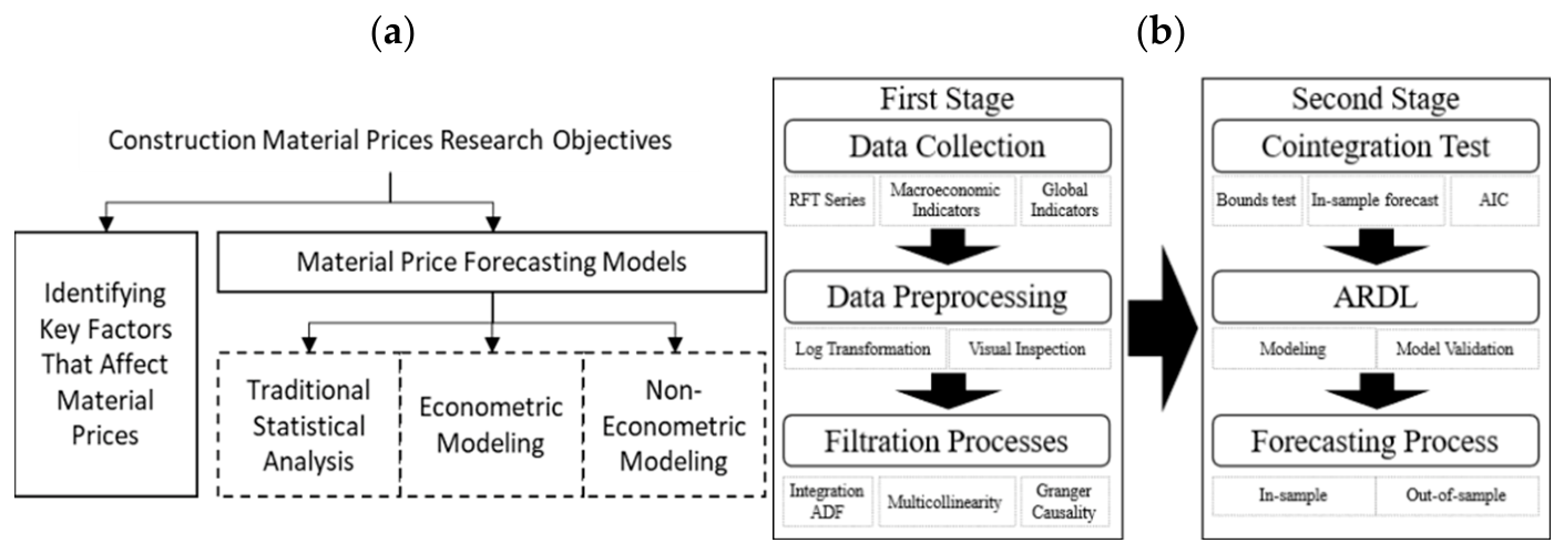
The research follows a two-stage multi-step framework (Figure 1). The first stage filters available macroeconomic variables to extract those with significant predictive power for building material prices. The second stage analyses the selected variables to model and forecast RFT prices using the ARDL framework. Each stage comprises three sub-processes, described in the subsections below.

The first-stage sub-processes are: (i) literature survey and data collection—candidate macroeconomic indicators are identified from the literature and collected from official Egyptian sources; (ii) data preprocessing—raw data are log-transformed to stabilise variance and normalise distributions; and (iii) variable filtering—the Augmented Dickey–Fuller (ADF) stationarity test, Variance Inflation Factor (VIF) multicollinearity check, and Granger causality test are applied sequentially to reduce the candidate set to statistically significant predictors.

The second-stage sub-processes are: (i) ARDL model specification—bounds testing is used to confirm cointegration and identify the optimal look-back period (LBP); (ii) model diagnostics—stability, linearity, homoscedasticity, and serial correlation tests validate model soundness; and (iii) forecasting evaluation—both in-sample and out-of-sample accuracy metrics assess model performance against OLS and VAR baselines.

An AI language assistance tool was used for copy-editing improvements to phrasing and structure in the preparation of this manuscript. All research content, analysis, results, and conclusions were generated by the authors.

2.1. Data Collection

Steel reinforcement bar is the most price-volatile major structural material in building construction and is extensively used in the literature to represent construction sector cost dynamics [12,29,30,32]. Given its 12–20% share of the structural budget noted earlier, its price is a critical input for building cost estimation and bid preparation. A pool of potential leading indicators from the published literature was selected as eligible for deployment in this prediction framework (

Table 1. Summary of economic indicators and independent variables by region.

Indicator	References	Region	Independent Variables
GDP	[30,32]	Egypt; US	Steel RFT and Portland Cement; Cement Prices
CPI/IR	[12,23,28,29,30,32,33]	Egypt; US; Taiwan; Pakistan; Nigeria	Steel RFT; Steel PPI; Taiwan CCI; Cement Prices; CCI; Mean Cost/m2
PPI	[30,32,33]	Egypt; US	Steel RFT; US CCI; Cement Prices
UR	[16,30]	Egypt; Australia	Steel RFT; Construction PPI (CPPI)
ER	[23,28,30,34]	Egypt; Taiwan; Nigeria; China	Steel RFT; Taiwan CCI; Cost/m2; Iron Ore
DR/LR	[16,23,26,28,30,32,34,35]	Egypt; Taiwan; Nigeria; Australia; US; China; India	RFT; Taiwan CCI; Cost/m2; CPPI; Steel; Ore; HCCI; Aluminium
ORE	[29,32]	US	Steel PPI; Steel Prices
Stock Index	[28]	Taiwan	Taiwan CCI
M0	[36,37]	US	Reinforced Concrete Pipe; Average Hourly Earnings

CCI = construction cost index; HCCI = highway CCI; PPI = producer price index; CPPI = construction PPI.

).

A study period from October 2009 to March 2024 was selected, containing 173 monthly observations. This period encompasses a range of destabilising events—including political unrest, currency devaluations, fuel price escalation, the COVID-19 pandemic, and geopolitical conflicts—making Egypt a representative case study context for investigating macroeconomic impacts on building material prices in an emerging market. The data were divided into training (October 2009–September 2023) and test (October 2023–June 2024) sets.

As presented in Table 1, various types of independent variables are employed in the literature, including economic variables such as the PPI, stock market, and M0; financial variables like the loan rate (LR) and discount rate (DR); and international variables like ORE and foreign stock market indexes.

Table 2. Summary of economic indicators with their ranges, frequencies, and sources.

Indicator	Range	Frequency	Source
Steel RFT	2950–52,000 EGP	Monthly	CAPMAS
GDP	1193–2149 billion EGP	Quarterly	CAPMAS
CPI	33.6–217 (index)	Monthly	CAPMAS
PPI	78.3–447 (index)	Monthly	CAPMAS
UR	6.7–13.4%	Quarterly	CAPMAS
POP	77.6–106.2 million	Monthly	CAPMAS
ER	5.5–47.2 EGP/USD	Monthly	CBE
LR	10–20%	Monthly	CBE
Discount Rate (DR)	8.5–27.8%	Monthly	CBE
Foreign Reserves (FRs)	13.4–45.5 billion USD	Monthly	CAPMAS
Trade Balance (TB)	1–5.1 billion EGP	Monthly	CAPMAS
EGX30	3622–28,964 (index pts)	Monthly	EG Stock
S&P500	524.4–5096.3 (index pts)	Monthly	NYSE
Hang Seng Index (HSI)	14,687–32,887 (index pts)	Monthly	Hong Kong Exchange
Iron Ore Price (ORE)	40.9–215.8 USD/tonne	Monthly	IMF (via FRED)
Money Supply (M0)	187,077–1,709,093 million EGP	Monthly	CBE

presents the available variable records in Egyptian databases.

2.2. Data Preprocessing

Applying a logarithmic transformation to the data helps make the distribution more normal by decreasing skewness, which is particularly useful in time series analysis as it stabilises the variance. The natural logarithm narrows the gap in the data range while preserving valuable information.

Table 3. Summary of economic indicators with their log-transformed ranges and means.

Indicator	Range (Log-Transformed)	Mean (Log-Transformed)
Steel RFT	7.99–10.86	9.09
GDP	7.08–7.67	7.34
CPI	3.51–5.40	4.30
PPI	4.36–6.17	5.02
UR	1.90–2.60	2.30
POP	4.35–4.66	4.52
ER	1.70–3.87	2.46
LR	2.23–3.21	2.57
Discount Rate (DR)	2.14–3.32	2.45
Foreign Reserves (FRs)	2.60–3.84	3.33
Trade Balance (TB)	−1.66–1.63	1.06
EGX30	8.19–10.27	9.15
S&P500	6.94–8.61	7.76
HSI	9.59–10.40	10.04
ORE	3.71–5.37	4.63
Money Supply (M0)	12.14–14.49	13.19

presents the log-transformed ranges and means.

2.3. Stationarity Test (ADF Test)

Stationarity is the property that describes a series with constant statistical properties such as mean and variance. The ARDL model accommodates a mixed order of integration, handling both stationary I(0) and integrated I(1) series. The Augmented Dickey–Fuller (ADF) test was used to investigate the variables’ order of integration. The null hypothesis H₀ is that the series contains a unit root (non-stationary); the alternative H_a assumes the series is stationary.

The test was performed in two sequential iterations. The first iteration tested the original series; if non-stationary, it proceeded to the second iteration in which the first difference was tested. If the difference in the series was stationary, it was classified as I(1). No I(2) variable was detected. Two variables showed stationarity in levels: Trade Balance (TB) and S&P500, both of which are I(0), and can be included in the ARDL without violating any modelling conditions as shown in

Table 4. Summary of ADF test results for economic indicators.

Series	Test Model	ADF t-Stat	SeriesΔ	Test Model	ADF t-Stat	Integration
Steel RFT	w/o const.	2.857	ΔRFT	with const.	−10.648 a	I(1)
GDP	w/const. & trend	−3.055	ΔGDP	with const.	−3.773 a	I(1)
PPI	w/o const.	4.016	ΔPPI	with const.	−8.806 a	I(1)
ER	w/o const.	2.443	ΔER	with const.	−12.086 a	I(1)
LR	w/o const.	1.166	ΔLR	w/o const.	−4.775 a	I(1)
DR	w/o const.	1.845	ΔDR	w/o const.	−6.365 a	I(1)
EGX30	w/const. & trend	−2.008	ΔEGX30	w/o const.	−13.073 a	I(1)
HSI	with const.	−2.037	ΔHSI	w/o const.	−14.476 a	I(1)
S&P500	w/const. & trend	−4.000 a	—	—	—	I(0)
Trade Balance (TB)	with const.	−4.990 a	—	—	—	I(0)
Money Supply (M0)	w/const. & trend	−3.157	ΔM0	with const.	−17.507 a	I(1)
ORE	with const.	−2.273	ΔORE	w/o const.	−9.982 a	I(1)

ᵃ Significant at 5%. Δ denotes first difference. I(0) = stationary in levels; I(1) = stationary after first differencing.

.

2.4. Multicollinearity Test

The Variance Inflation Factor (VIF) was adopted to identify multicollinearity in the model. The proposed full model is presented in Equation (1):

$$\Delta RFT=C_0+C_1\Delta GDP+\cdots +C_{22}\Delta M0$$

(1)

As presented in

Table 5. Variance Inflation Factor (VIF) for economic indicators.

Indicator	VIF
PPI	2.409
ER	1.907
LR	2.638
DR	2.626
EGX30	3.673
S&P500	1.206
HSI	1.297
ORE	1.187
M0	1.065
Fuel 92 (excluded)	10.590
Fuel 80 (excluded)	9.019

VIF > 10 indicates severe multicollinearity; those variables were excluded.

, fuel price variables (gasoline 92 and 80) exceeded VIF > 10 and were excluded. Egyptian stock market sub-indices (EGX70, EZZ, EGST) showed interdependence but did not reach multicollinearity levels; they were excluded following the principle of parsimony.

The VIF > 10 exclusion threshold follows the standard econometric rule of thumb; O’Brien [38] cautions against mechanically applying stricter cutoffs such as VIF > 5, showing that moderate VIF values do not by themselves invalidate coefficient estimates. In this application, the choice of threshold is, in any case, not binding: all retained indicators exhibit VIF < 4 (Table 5), comfortably below even the stricter standard.

2.5. Granger Causality Test

The Granger causality test was performed on different lags (2, 4, 6, 8, 10, and 12 months) between RFT and the tested variables. When the test statistics are significant at the 5% level, the independent variable at that specific lag is considered to Granger-cause the dependent variable and can be used to predict future RFT prices. Two design decisions in the lag structure warrant explanation. First, the Granger causality screening was performed at even lags (2, 4, …, 12 months) as a horizon-coverage scan rather than a lag-optimisation exercise: its purpose was to establish whether predictive content exists at short, medium, and long horizons, and coarser spacing preserves test power in a finite sample by limiting the number of estimated coefficients per test. Second, the maximum boundary of 12 months is consistent with the lead–lag horizons reported for construction leading indicators [22,30] and with the conventional view that monetary and exchange-rate shocks are transmitted to domestic prices within approximately one year. See

Table 6. Granger causality test statistics for selected lag lengths.

Null Hypothesis	Lag 2	Lag 4	Lag 6	Lag 8	Lag 10	Lag 12
ΔPPI ΔRFT	1.273	0.959	2.481 *	2.032 *	1.696 *	1.391
ΔER ΔRFT	5.034 **	3.353 **	2.390 *	1.708	1.402	1.367
ΔLR ΔRFT	5.530 **	3.719 **	3.345 **	2.648 **	2.045 *	2.096 *
ΔDR ΔRFT	3.252 *	1.834	2.645 *	2.027 *	1.533	1.324
ΔORE ΔRFT	4.907 **	2.701 *	1.186	1.862	1.512	1.378
ΔEGX30 ΔRFT	3.214 *	1.875	2.433 *	2.035 *	2.017 *	1.835 *
ΔS&P500 ΔRFT	1.440	1.942	2.321 *	2.523 *	2.584 **	2.285 *
ΔHSI ΔRFT	0.161	0.268	0.417	0.696	2.535 **	2.135 *
ΔM0 ΔRFT	0.494	1.139	2.249 *	1.939	1.427	1.321

* p < 0.05; ** p < 0.01. F-statistics shown. denotes ‘does not Granger cause’.

.

The Granger causality test identified nine significant predictors: PPI, exchange rate (ER), loan rate (LR), discount rate (DR), iron ore prices (ORE), Egyptian Stock Market Index (EGX30), American Stock Market Index (S&P500), Hang Seng Index (HSI), and money supply (M0). The filtering pipeline reduced the candidate variable set to these nine predictors (

Table 7. Summary of selected variable types and sources.

Variable Type	Variable	Source
Dependent Variable	Steel RFT Prices	CAPMAS
Independent Variable	PPI	CAPMAS
Independent Variable	ER	CBE
Independent Variable	LR	CBE
Independent Variable	Discount Rate (DR)	CBE
Independent Variable	Iron Ore Price (ORE)	IMF (via FRED)
Independent Variable	EGX30	Egypt Exchange
Independent Variable	S&P500	US Exchange
Independent Variable	HSI	Hong Kong Exchange
Independent Variable	Money Supply (M0)	CBE

).

2.6. Cointegrated Variable Selection

The Granger causality test captured short-term relationships. For long-term relationships, a cointegration test is required. Cointegration describes the case in which two or more time series share a linear combination that moves stably in the long run [39,40]. This research utilised the ARDL model, which accommodates a mixed-order integration process aligned with the collected data characteristics. It offers a flexible lag-selection process using different lags for the dependent and independent variables and can accommodate small samples.

A non-linear extension of the framework (NARDL) was considered, in which positive and negative partial-sum decompositions of the regressors allow asymmetric short- and long-run responses [41]. Three considerations favoured the linear specification. First, the partial-sum decomposition doubles the number of distributed-lag regressors; with 168 training observations and lag orders of up to twelve, the resulting loss of degrees of freedom would be prohibitive for reliable bounds inference. Second, the dominant source of asymmetry in the sample—the discrete 2022 regime shift—is captured directly by the structural break dummy rather than left to be absorbed by asymmetric slope coefficients. Third, the Ramsey RESET results reported in Section 3.3 fail to reject the null of correct linear specification for all three look-back periods, providing direct statistical evidence that a linear functional form is an acceptable simplification for this dataset. Asymmetric price transmission—in particular the possibility that RFT prices rise faster than they fall—remains a promising avenue for future work.

The look-back period (LBP) was defined as the lag period between the dependent variable RFT and the independent variables. The candidate LBPs of 3, 6, and 9 months were fixed ex ante on practical rather than statistical grounds: they correspond to the quarterly tender-preparation cycle, the semi-annual budget review, and the typical lead time for bulk procurement scheduling in Egyptian building projects. Pre-specifying the forecast horizons in this way, rather than selecting them by searching over neighbouring values, avoids data-snooping in horizon choice; conditional on each LBP, the lag order of every variable was then selected by minimising the Akaike Information Criterion (AIC). During this variable-selection stage, the framework fixes the LBP to 0, the deterministic variable to an unconstrained constant, the dependent variable lags up to 2, and independent variable lags up to 12.

Table 8. Summary of model comparisons with AIC, F-Bounds, and t-Bounds during stepwise variable selection.

Variables	Model	AIC	F-Bounds	t-Bounds
RFT + PPI	ARDL(2,1)	5.114 *	—	−3.193 *
+ER	ARDL(2,1)	−2.973	10.529 **	−4.407 **
+HSI	ARDL(2,0,7)	−3.132	15.383 **	−6.189 **
+S&P500	ARDL(2,0,7)	−3.119	15.271 **	−6.033 **
+M0	ARDL(2,9,6,1)	−3.059	7.042 **	−4.565 **
+LR	ARDL(2,9,6,1)	−3.053	6.614 **	−4.588 **

* Significant at 5%; ** Significant at 1%.

shows the stepwise selection results. The combination of PPI, ER, HSI, S&P500, M0, and LR satisfies the cointegrated ARDL requirements. The resulting model-level AIC values are reported alongside the selected model parameters in

Table 9. Summary of ARDL model parameters for different look-back periods (LBPs).

Variable	LBP = 3 Lags	LBP = 3 Params	LBP = 6 Lags	LBP = 6 Params	LBP = 9 Lags	LBP = 9 Params
RFT	2 [−1, −2]	1.023; −0.271	2 [−1, −2]	1.083; −0.305	2 [−1, −2]	1.080; −0.282
Constant	—	0.479	—	1.799	—	2.022
PPI	12 [−3, −15]	0.366 to 0.174	9 [−6, −15]	0.381 to −0.398	7 [−9, −16]	0.158 to −0.083
HSI	8 [−3, −11]	0.172 to −0.120	6 [−6, −12]	0.050 to −0.135	4 [−9, −13]	−0.307 to −0.160
M0	1 [−6, −7]	0.005; 0.282	1 [−6,−7]	−0.014; 0.213	0 [−9]	0.211
ER	0 [−3]	−0.010	0 [−6]	0.068	0 [−9]	0.101
S&P500	0 [−3]	−0.150	0 [−6]	−0.088	0 [−9]	−0.080
LR	0 [−3]	−0.013	0 [−6]	−0.037	0 [−9]	−0.064
AIC	—	−3.088	—	−3.053	—	−3.008

.

2.7. Deterministic Term Selection

The ARDL model distinguishes between three cases for model parameters: with a trend and constant, with only a constant, and without a trend or constant. According to Jiang et al. [16], the first and third cases are considered impractical for this dataset. This research relied on the case with only a constant in the model.

2.8. Benchmark Models

To contextualise the ARDL’s forecasting performance, two multivariate benchmarks were estimated on the identical training sample (October 2009–September 2023): an OLS regression and a vector autoregression (VAR). Because the dataset combines I(0) and I(1) series (Table 4), a levels VAR would be spurious and a VECM inadmissible; the VAR was therefore specified in first differences, with the I(0) S&P500 entered in levels. The endogenous system comprised ΔRFT, ΔPPI, ΔER, ΔHSI, S&P500, ΔM0, and ΔLR, with a constant and the 2022M07 structural break dummy as exogenous terms, mirroring the ARDL treatment. All lag-length criteria (FPE, AIC, SC, HQ) unanimously selected an order of one; a VAR(2) was tested under a pre-committed decision rule and rejected, as it failed to improve the residual autocorrelation profile. All inverse roots of the characteristic polynomial lie inside the unit circle (maximum modulus 0.992, attributable to the persistence of the S&P500 series in levels), satisfying the stability condition. Dynamic out-of-sample forecasts of ΔRFT were cumulated from the September 2023 log-level to reconstruct level forecasts over the test window.

3. Results

3.1. Selected Models

The preceding stages resulted in nine models, one per look-back period. Table 9 presents the models for LBP = 3, 6, and 9. Each ARDL model consists of a long-term and a short-term relationship, with the cointegration relationship presented in

Table 10. Summary of Error Correction Model (ECM) parameters.

Variable	LBP = 3 Lags	LBP = 3 Params	LBP = 6 Lags	LBP = 6 Params	LBP = 9 Lags	LBP = 9 Params
COINTEQ *	—	−0.248 (0.000)	—	−0.222 (0.000)	—	−0.202 (0.000)
ΔRFT	—	0.271	—	0.305	—	0.282
ΔPPI	[−3, −14]	see Table 9	[−6, −14]	see Table 9	[−9, −15]	see Table 9
ΔHSI	[−3, −10]	see Table 9	[−6, −11]	see Table 9	[−9, −12]	see Table 9
ΔM0	[−3]	0.005	[−6]	−0.014	—	—

COINTEQ * = cointegrating equation coefficient (speed of adjustment). p-values in parentheses.

.

These models provide both long-run and short-run relationships between the RFT and the candidate variables. The cointegration term is significant in all nine models. For LBP  =  3, the system corrects short-term shocks by 24.8% per period, suggesting that if a shock disturbs the equilibrium price, it takes approximately 4 months to return to equilibrium. The cointegration equations for LBP  =  3, 6, and 9 are presented in Equations (2)–(4), where CE denotes the cointegrating equation:

$$CE=\Delta RFT-\left(0.4954\cdot PP{I}_{-4}-0.5346\cdot HS{I}_{-4}+1.1327\cdot M{0}_{-4}\right)$$

(2)

$$CE=\Delta RFT-\left(0.3246\cdot PP{I}_{-7}-0.9248\cdot HS{I}_{-7}+0.8672\cdot M{0}_{-7}\right)$$

(3)

$$CE=\Delta RFT-\left(0.0595\cdot PP{I}_{-10}-1.5576\cdot HS{I}_{-10}+1.2517\cdot M{0}_{-9}\right)$$

(4)

3.2. Model Stability (CUSUM and CUSUMSQ Tests)

CUSUM and CUSUMSQ tests assessed the stability of the model parameters.

Table 11. Summary of model stability results (CUSUM and CUSUMSQ tests).

LBP	Model	CUSUM	CUSUMSQ
3	ARDL(2,12,8,1)	Stable	Unstable at 2022M01
6	ARDL(2,9,6,1)	Stable	Stable
9	ARDL(2,7,5,0)	Stable	Unstable at 2017M02 and 2022M01

presents the inference from the test plots. A structural break in January 2022 was identified, consistent with the Egyptian foreign currency crisis and post-COVID global shocks. Individual series tested separately (

Table 12. Summary of structural breakpoint tests on individual series.

Series	CUSUMSQ Stability	Break Point
Steel RFT	Unstable	2022M07
CPI	Unstable	2022M10
PPI	Unstable	2022M11
ER	Unstable	2022M05
LR	Unstable	2022M07
DR	Unstable	2022M09
ORE	Unstable	2022M05
EGX30	Unstable	2022M05
S&P500	Unstable	2020M11
HSI	Unstable	2021M05
Money Supply (M0)	Unstable	2022M01

All series exhibit a structural break concentrated around 2022, consistent with the Egyptian foreign currency crisis and post-COVID global shocks.

) confirmed a structural break concentrated around 2022. A dummy variable covering July 2022 to the end of the sampling period was introduced; its start date was anchored to the breakpoint of the RFT series itself (2022M07, Table 12) rather than the earlier model-level instability date, since it is the dependent variable’s own regime shift that the specification must absorb. Formally, the dummy is a step (intercept) variable, defined as D_t = 0 for t < 2022M07 and D_t = 1 thereafter, entering the specification as an additive fixed regressor: it shifts the intercept of the level relationship—equivalently, the long-run mean around which the cointegrating relationships in Equations (2)–(4) hold—in the post-break regime, leaving the slope coefficients unchanged. A step form was preferred to a gradual trend break because the underlying event—the foreign-currency crisis and its associated devaluation steps—constituted a discrete regime change rather than a smooth transition, consistent with the CUSUMSQ evidence of instability concentrated at a point in time. Sample splitting was rejected because the post-break segment of the training sample (approximately 15 monthly observations) is too short for independent estimation, and regime-switching specifications were set aside on the same degrees-of-freedom grounds discussed for the NARDL alternative in Section 2.6.

Table 13. Summary of model statistics and stability after dummy variable inclusion.

LBP	Model	F-Statistic	t-Statistic	CUSUMSQ After Dummy
3	ARDL(2,12,8,1)	7.549 **	−4.307 *	Stable
6	ARDL(2,9,6,1)	6.541 **	−4.445 **	Stable
9	ARDL(2,7,5,0)	6.977 **	−3.931 *	Stable

* Significant at 5%; ** significant at 1%.

shows the models gaining stability while retaining cointegration significance.

3.3. Linearity, Heteroskedasticity, and Serial Correlation Tests

The Ramsey RESET Specification test was performed to examine model robustness.

Table 14. Ramsey RESET specification test results.

LBP	Model	t-Stat (p)	F-Stat (p)	Conclusion
3	ARDL(2,12,8,1)	0.102 (0.919)	0.010 (0.919)	Correctly Specified
6	ARDL(2,9,6,1)	1.096 (0.275)	1.200 (0.275)	Correctly Specified
9	ARDL(2,7,5,0)	0.501 (0.617)	0.251 (0.617)	Correctly Specified

presents consistent linear behaviour between the steel RFT and the proposed regressors. The Breusch–Pagan–Godfrey and ARCH tests (

Table 15. Breusch–Pagan–Godfrey and ARCH heteroskedasticity test results.

LBP	Model	Breusch–Pagan–Godfrey (p)	ARCH Test (p)
3	ARDL(2,12,8,1)	28.567 (0.540)	0.465 (0.495)
6	ARDL(2,9,6,1)	28.900 (0.268)	0.847 (0.358)
9	ARDL(2,7,5,0)	24.560 (0.267)	0.079 (0.779)

) confirmed homoscedasticity of residual variance across all LBPs, ensuring reliable standard errors. The Breusch–Godfrey Serial Correlation LM Test (

Table 16. Breusch–Godfrey serial correlation LM test results.

LBP	Model	LM: 4 Lags (p)	LM: 8 Lags (p)	LM: 12 Lags (p)	Correlogram Q-Stat
3	ARDL(2,12,8,1)	4.394 (0.355)	12.088 (0.147)	16.073 (0.188)	No Serial Corr.
6	ARDL(2,9,6,1)	6.238 (0.182)	12.585 (0.127)	15.501 (0.215)	No Serial Corr.
9	ARDL(2,7,5,0)	1.146 (0.887)	4.863 (0.772)	5.674 (0.932)	No Serial Corr.

H₀: No Serial Correlation. Failure to reject confirms well-specified residuals.

) confirmed no serial correlation in the model residuals.

3.4. Forecasting Accuracy Metrics

The root mean square error (RMSE), mean absolute percentage error (MAPE), mean absolute error (MAE), and Theil’s Inequality Coefficient (U₁) were utilised to assess forecasting power; RMSE, MAE, and MAPE are defined in Equations (5)–(7). A lower RMSE indicates predictions closer to actual values. A lower MAPE (%) indicates better performance. MAE is less sensitive to outliers than MAPE. U₁ considers both the magnitude and direction of forecast errors; zero indicates a perfect forecast; one indicates the forecast is no better than a naïve forecast. Following best practice, U₁ is further decomposed into bias, variance, and covariance proportions.

$$RMSE=\sqrt{{\displaystyle \frac{{\sum }_{i=1}^N{\left(x_i-{\widehat{x}}_i\right)}^2}{N}}}$$

(5)

$$MAE={\displaystyle \frac{{\sum }_{i=1}^N\left|{\widehat{x}}_i-x_i\right|}{N}}$$

(6)

$$MAPE={\displaystyle \frac{100}{N}}{\displaystyle {\displaystyle \sum }_{i=1}^N}\left|{\displaystyle \frac{x_i-{\widehat{x}}_i}{x_i}}\right| (\%)$$

(7)

where i is the observation number, N is the number of data points, x_i is the actual observation, and ${\widehat{\mathrm{x}}}_{\mathrm{i}}$ is the ARDL model estimate. Note that all MAPE values are reported in log-transformed space; equivalent price-space percentage deviations are obtained by back-transformation as exp(MAE) − 1 and exp(RMSE) − 1 (see Section 4).

3.5. In-Sample Forecasting

The ARDL model was evaluated for three look-back periods: LBP  =  3, 6, and 9 (Figure 2). In-sample accuracy was broadly similar across the three look-back periods (RMSE 0.075–0.086 in log space). As the LBP increased to 6 and 9, forecasts experienced more smoothness but with a drift from the original RFT series, attributable to the model’s longer memory. The in-sample accuracy is satisfactory (

Table 17. Performance metrics for selected models: in-sample forecast.

LBP	Model	RMSE	MAPE (%)	MAE	U1
3	ARDL(2,12,8,1)	0.0786	0.67	0.0609	0.0043
6	ARDL(2,9,6,1)	0.0753	0.69	0.0625	0.0041
9	ARDL(2,7,5,0)	0.0856	0.80	0.0722	0.0047

RMSE and MAE in log-transformed units (dimensionless). MAPE expressed as a percentage.

). The U₁ coefficient is approximately zero for all LBPs, and its decomposition attributes the in-sample errors almost entirely to the unsystematic covariance component (bias proportion < 0.001), indicating non-biased in-sample forecasts.

Table 18. Comparison of ARDL and OLS baseline: in-sample forecasting.

Metric	LBP = 3 ARDL	LBP = 3 OLS	LBP = 6 ARDL	LBP = 6 OLS	LBP = 9 ARDL	LBP = 9 OLS
AIC	−3.075	−1.446	−3.040	−1.181	−3.006	−0.890
RMSE	0.0786	0.1126	0.0753	0.1284	0.0856	0.1484
MAE	0.0609	0.0850	0.0625	0.0975	0.0722	0.1241

shows a comparison of ARDL and OLS baseline: in-sample forecasting.

Figure 2. In-sample forecasting performance: full sample period (October 2009–September 2023). The grey-shaded region indicates the magnified sub-period shown in Figure 3.

Figure 2. In-sample forecasting performance: full sample period (October 2009–September 2023). The grey-shaded region indicates the magnified sub-period shown in Figure 3.

Figure 3. In-sample forecasting performance: magnified view (December 2014–March 2018). (a) LBP  =  3; (b) LBP  =  6; (c) LBP  =  9.

Figure 3. In-sample forecasting performance: magnified view (December 2014–March 2018). (a) LBP  =  3; (b) LBP  =  6; (c) LBP  =  9.

3.6. Out-of-Sample Forecasting

Out-of-sample forecasting was evaluated on the held-out dataset beginning October 2023 to guard against overfitting. Each model was assessed over its designated horizon as a genuine multi-step (dynamic) forecast generated from the end of the training sample: LBP  =  3 over October–December 2023, LBP  =  6 over October 2023–March 2024, and LBP  =  9 over October 2023–June 2024. The test window contains the sharpest price movement in the sample—a surge of roughly 20% between December 2023 and February 2024 followed by a partial retreat—making it a demanding stress test for any forecasting specification. The 3-month model performed best (RMSE 0.0672 in log space), while the 6- and 9-month models, whose horizons spanned the surge, recorded larger errors (

Table 19. Performance metrics for selected models: out-of-sample forecast.

LBP	Model	RMSE	MAPE (%)	MAE	U1
3	ARDL(2,12,8,1)	0.0672	0.54	0.0569	0.0032
6	ARDL(2,9,6,1)	0.1503	1.19	0.1274	0.0071
9	ARDL(2,7,5,0)	0.1403	1.05	0.1126	0.0066

RMSE and MAE in log-transformed units; MAPE computed on the log-transformed series. Each model is evaluated over its designated horizon as a dynamic multi-step forecast (Section 3.6). Back-transformed price-space equivalents (exp(metric) – 1): LBP = 3, MAE ≈ 5.9%, RMSE ≈ 7.0%; LBP = 6, MAE ≈ 13.6%, RMSE ≈ 16.2%; LBP = 9, MAE ≈ 11.9%, RMSE ≈ 15.1%.

); the 9-month model partially recovered by the end of its window as prices retreated toward the forecast path (Figure 4a). Compared with the OLS model, the ARDL model (Figure 4b) tracked the RFT trend, whereas the OLS model provided a near-constant forecast. The U₁ coefficients remained close to zero in absolute terms; however, their decomposition showed that the out-of-sample errors at the longer horizons contained a substantial systematic component, reflecting under-prediction of the early-2024 surge—a devaluation-driven shock whose magnitude no linear specification could anticipate from information available at the forecast origin.

Table 20. Comparison of ARDL and OLS baseline: out-of-sample forecasting.

Metric	LBP = 3 ARDL	LBP = 3 OLS	LBP = 6 ARDL	LBP = 6 OLS	LBP = 9 ARDL	LBP = 9 OLS
RMSE	0.0672	0.0832	0.1503	0.1301	0.1403	0.1310
MAE	0.0569	0.0765	0.1274	0.0990	0.1126	0.0988

MAPE computed on the log-transformed series. ARDL metrics are dynamic multi-step forecasts over each model’s designated horizon (Section 3.6); OLS metrics are evaluated over the full October 2023–June 2024 window. The ARDL retains a clear advantage at the 3-month horizon.

Illustrates a comparison of ARDL and OLS baseline: out-of-sample forecasting.

The VAR(1) benchmark was evaluated over October 2023–March 2024, which coincides with the 6-month ARDL horizon;

Table 21. Out-of-sample comparison of ARDL, OLS, and VAR benchmarks (October 2023–March 2024).

Metric	ARDL (LBP = 6)	OLS (LBP = 3)	VAR(1)
RMSE (log space)	0.1503	0.0832	0.1501
MAE (log space)	0.1274	0.0765	0.1264
MAPE, price space (%)	≈13.6	≈8.0	≈11.6

Price-space errors obtained by back-transforming forecasts to levels before computing percentage deviations; see the note following Equation (7). ARDL statistics are the dynamic 6-month-horizon results from Table 19, matching the VAR evaluation window (October 2023–March 2024); OLS statistics are as reported in Table 20 (full test window).

therefore compares the models over this common window in log space and in back-transformed price space, with the OLS baseline shown for reference. Over the common window, the dynamic ARDL (LBP  =  6) and the VAR recorded nearly identical errors (RMSE 0.1503 and 0.1501, respectively): both under-predicted the early-2024 surge—the VAR because its dynamic forecast converges to the model’s unconditional mean growth within three steps, and the ARDL because the error-correction pull operates too gradually to absorb a shock of this size within six months. Estimation in first differences nevertheless carries a structural cost: it discards the long-run cointegrating relationship confirmed by the bounds test, leaving the VAR without an equilibrium anchor at any horizon. The ARDL’s advantage is accordingly concentrated at its 3-month design horizon (RMSE 0.0672; price-space MAE ≈ 5.9%; Table 19)—the horizon most relevant to tender preparation—where the cointegration anchor contributes before multi-step uncertainty accumulates. In price terms, the 6-month errors of both multivariate models (≈11.6–13.6% MAE) approached the upper bound of the 10–15% contingency band typical of Egyptian structural budgets, reinforcing that horizons beyond one quarter are better suited to directional planning than to firm price commitments. The full decomposition of the U₁ statistic for the in-sample and out-of-sample forecasts is reported in

Table 22. Decomposition of Theil’s U₁ statistic into bias, variance, and covariance proportions.

LBP	Sample	Bias Proportion	Variance Proportion	Covariance Proportion
3	In-sample	0.0001	0.0078	0.9921
6	In-sample	0.0000	0.0058	0.9942
9	In-sample	0.0000	0.0208	0.9792
3	Out-of-sample	0.3915	0.5184	0.0901
6	Out-of-sample	0.6849	0.2831	0.0320
9	Out-of-sample	0.5250	0.0298	0.4452

Proportions sum to unity for each forecast. In-sample errors are almost entirely unsystematic (covariance proportion > 0.98). The out-of-sample proportions at LBP = 3, 6, and 9 are computed over 3, 6, and 9 observations, respectively, and should be read as descriptive; the elevated bias proportions reflect systematic under-prediction of the early-2024 price surge discussed in Section 3.6.

.

4. Discussion

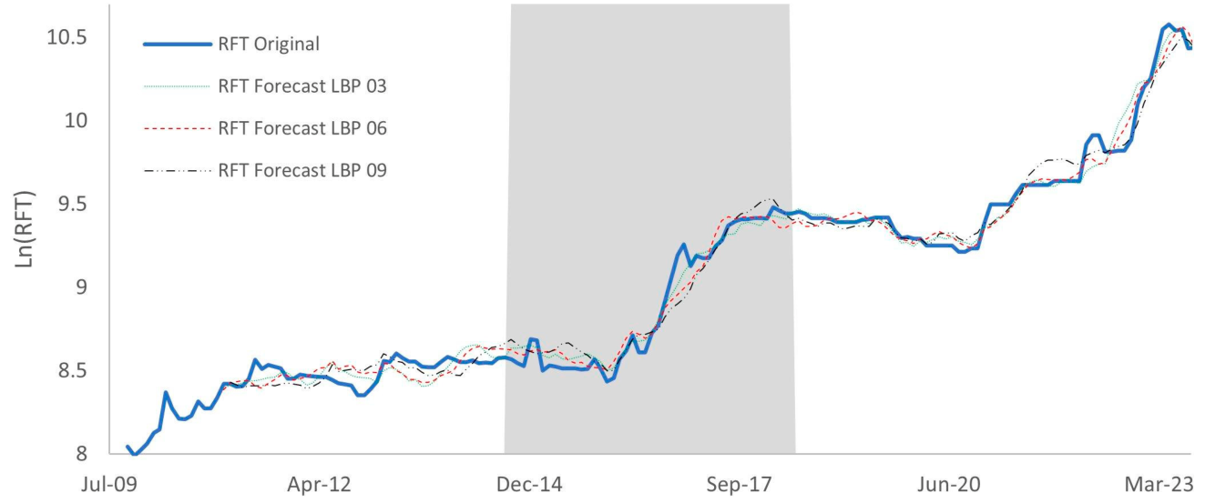
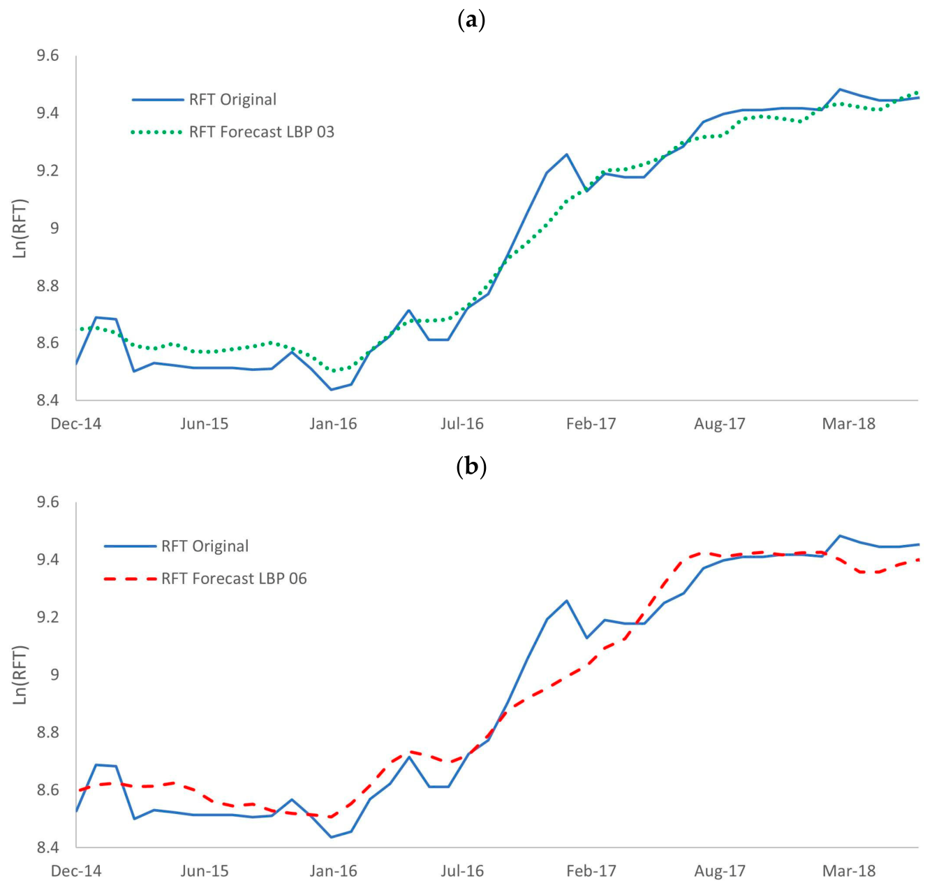
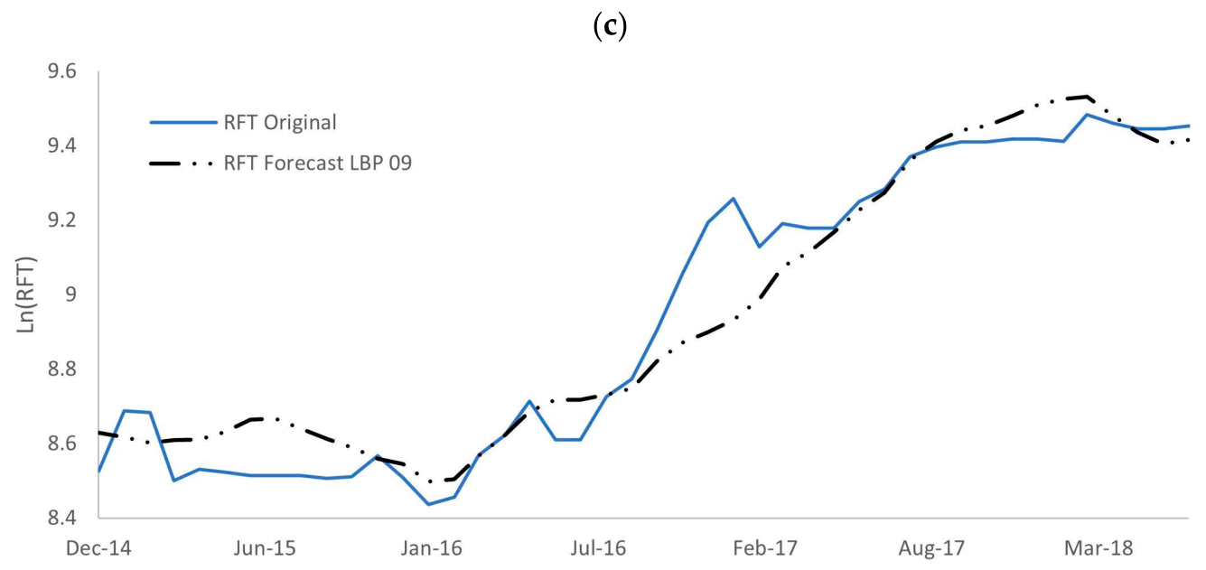
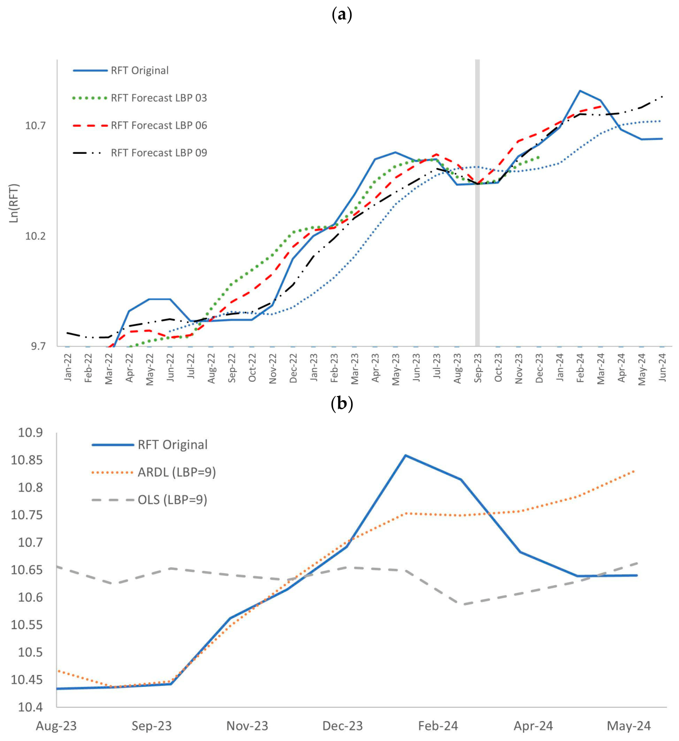
The ARDL model developed in this study demonstrated strong forecasting capability for Egyptian RFT prices, outperforming the OLS baseline at the 3-month horizon that matters most for tender preparation. The out-of-sample errors must be interpreted relative to building cost management practice rather than as an abstract statistical benchmark. In Egyptian building construction, contingency allowances for structural materials typically range from 10–15% of the structural cost budget. Because all error metrics are computed on natural-log-transformed prices, the reported MAPE overstates the practical forecast error: dividing absolute log-space errors by log-price levels (approximately 8–11) inflates the percentage figure. Back-transforming the out-of-sample errors to price space, the LBP  =  3 model’s MAE of 0.0569 log units corresponds to a typical price deviation of approximately 5.9% (exp(0.0569) − 1), and its RMSE of 0.0672 to approximately 7.0%; at the longer horizons, which span the early-2024 surge, the price-space deviations rise to roughly 11.9–13.6% (MAE). At the 3-month horizon most relevant to tender preparation, the expected price deviation of 5.9–7.0% falls within the 10–15% contingency band, leaving a residual-risk margin of roughly 3–9 percentage points; by contrast, the OLS baseline’s back-transformed error (approximately 8.0% MAE and 8.7% RMSE over the full test window) consumes most of that band. At the 6- and 9-month horizons, the expected deviations approach or reach the band itself, so those forecasts inform market direction and procurement timing rather than firm budget figures. The framework thus provides actionable budget guidance rather than precise prediction, which is the appropriate standard for a volatile emerging-market commodity. In contract terms, the 3-month forecast is accurate enough to inform contingency-setting in fixed-price (lump-sum) bids, since the expected deviation sits inside the customary buffer; the 6- and 9-month horizons, with larger price-space errors, are better suited to cost-plus arrangements, feasibility-stage budget sizing, and procurement-timing decisions than to firm price commitments. Egypt experienced approximately 50% Egyptian pound depreciation between 2022 and 2024, a period characterised by unprecedented currency volatility, fuel price escalation, and geopolitical disruption [3,11]. Under such conditions, the ARDL framework—which explicitly models the 2022 structural break via a dummy variable—provides a substantially more reliable basis for building cost planning than naïve estimation or static regression. The VAR comparison reinforces this conclusion from a different direction: a differenced VAR, the only admissible VAR specification for mixed-integration data, forfeits the long-run equilibrium information that the ARDL retains, and its forecast accuracy deteriorates accordingly (Table 21).

Comparison with the closest prior study—Shiha et al. [30], who applied ANN models to Egyptian RFT and Portland cement prices—reveals important advances. While Shiha et al. reported MAPE values of 4–11%, their dataset (2008–2018) predated the structural breaks of 2022. The present study explicitly models this structural break using a dummy variable, extending the validated framework to the most volatile period in Egypt’s modern economic history. Furthermore, the ARDL framework handles the mixed stationarity of economic time series—a combination of I(0) and I(1) variables—that standard regression and VECM approaches cannot accommodate without additional transformation. This is a fundamental methodological advantage over prior Egyptian market studies.

The selection of international stock indices (S&P500 and HSI) as Granger-causal predictors of Egyptian RFT prices reflects the globalised nature of steel markets. Egyptian steel production depends heavily on imported scrap iron, whose price co-moves with international equity markets. The inclusion of these globally traded indicators distinguishes this framework from Egypt-centric models and improves its sensitivity to external shocks. The PPI and money supply (M0) predictors are consistent with prior international literature [16,32], providing external validity to the filtering results.

The cointegrating equations (Equations (2)–(4)) reveal that PPI exerts a positive long-run effect on RFT prices, consistent with the role of production costs in steel pricing. HSI exhibits a negative long-run coefficient, and the financialization channel supplies a concrete mechanism. Egyptian mills rely on imported ferrous scrap and billet priced in US dollars, and the HSI proxies Asian—particularly Chinese—industrial demand conditions. When Asian equity markets rise, signalling expanding industrial activity and global risk appetite, scrap and billet cargoes are bid toward East Asian buyers, raising the landed cost faced by Egyptian importers precisely when foreign-currency availability in Egypt is under pressure. Egyptian steel producers thus compete in the same international scrap market as Chinese demand, and the equity index transmits this competition into domestic RFT prices with a lag—the cross-market transmission mechanism described in the commodity financialization literature [14,15]. The speed of adjustment coefficient (−0.248 for LBP  =  3) implies that approximately 24.8% of any deviation from long-run equilibrium is corrected each month, returning to equilibrium in approximately 4 months—a practically relevant horizon for contractor procurement planning. To translate this into a contractor’s timeline: consider a bid submitted with a standard 30-day validity window immediately after an adverse price shock, such as a sudden devaluation-driven RFT spike. The estimated adjustment speed implies that only about a quarter of the disequilibrium dissipates within that window, so the contractor cannot rely on prices reverting before award and should price the bid at close to the shocked level, expecting only partial relief over the following quarter. Conversely, a cost consultant advising on procurement timing after such a spike can anticipate that the bulk of the excess will unwind over roughly four months, which argues for deferring non-critical bulk purchases beyond the immediate post-shock period where the programme allows.

In building project delivery, price risk management occurs at three critical stages: schematic design, when the structural material budget is established; tender preparation, when contractors price their bids against current and projected market rates; and procurement, when purchase orders are placed against a fluctuating market. The 3-month ARDL forecast is most applicable at the tender preparation stage, where a forward-looking price estimate enables building contractors to include a data-driven RFT contingency in their bid rather than relying on experience-based judgment. The 9-month forecast supports procurement scheduling—allowing building projects to anticipate market direction and time bulk RFT purchasing to projected lower-price periods. The integration of this model into quantity surveying practice would require only monthly data feeds from CAPMAS and CBE, both of which are publicly available, making operational deployment technically feasible without proprietary data access.

A practical caveat concerns institutional reporting lags. CAPMAS and CBE releases typically become available one to two months after the reference month, so a nominal 3-month-ahead forecast issued from the latest available data is, in real time, an effective 1–2-month forward-looking estimate. Practitioners can navigate this in two ways: for tender preparation, the LBP = 3 model should be run on the most recent complete data vintage and interpreted as a near-term price check on current quotations; for budget-setting and procurement scheduling, the LBP = 6 and LBP = 9 models are more robust to the lag, since a two-month erosion of a 9-month horizon still leaves a genuinely forward-looking 7-month window. Where a single predictor is delayed, its most recent available observation can be carried forward as a nowcast, at the cost of modest additional uncertainty.

The primary limitations of this study are fourfold. First, the model assumes linear and symmetric relationships between macroeconomic indicators and RFT prices; although the RESET tests support this specification in-sample, asymmetric adjustment and regime-switching behaviour during extreme market episodes may not be fully captured, and a NARDL extension [41] is a natural next step. Second, the dataset ends March 2024; the model’s performance during any subsequent structural break remains unvalidated. Third, forecast errors grow materially with horizon: while the 3-month model’s price-space error (≈5.9% MAE) is comparable to the 4–11% MAPE reported by ANN-based studies on calmer pre-2020 data, the 6- and 9-month errors (≈12–14% MAE) approach the upper bound of customary contingency allowances—a gap that future hybrid ARDL–LSTM approaches could partially close [42]. Fourth, the framework inherits the publication lag of its inputs, as discussed above, which compresses the effective forecast horizon available to practitioners in real time. Future research should test the framework’s transferability to other building material prices (cement, aggregate, formwork, glazing) and to other emerging-market construction economies where monthly macroeconomic data are available.

5. Conclusions

This study developed and validated an ARDL-based forecasting framework for steel reinforcement bar (RFT) prices in Egypt—a building construction market characterised by severe macroeconomic volatility, mixed-stationarity economic data, and a documented structural break in 2022. The framework provides actionable 3-, 6-, and 9-month price forecasts using nine macroeconomic leading indicators identified through a reproducible variable-selection pipeline (stationarity testing, VIF multicollinearity screening, and Granger causality testing) and validated through comprehensive model diagnostics including CUSUM stability tests, Ramsey RESET specification testing, heteroskedasticity checks, and serial correlation tests.

At the operationally critical 3-month horizon, the ARDL demonstrated superiority over OLS in both understanding data dynamics and capturing the data generation process, achieving, in genuine multi-step evaluation, an out-of-sample price-space error of approximately 5.9% (mean absolute) under crisis-period conditions, versus approximately 8% for the OLS baseline. This superior performance highlights the advantages of the ARDL framework in capturing both short-run dynamics and long-run equilibrium relationships within the complex interplay of macroeconomic variables influencing steel prices. The first-difference VAR(1) benchmark performed worse still (Table 21), confirming that the long-run cointegrating information retained by the ARDL is central to its forecasting advantage.

For building project teams, the ARDL framework delivers RFT price forecasts at 3-, 6-, and 9-month horizons. The 3-month forecast is most directly applicable at the tender preparation stage of reinforced concrete building projects, where a validated forward price indicator reduces reliance on experience-based contingency setting, improves bid accuracy and competitiveness in volatile procurement markets, and reduces post-contract cost overrun exposure. The 9-month forecast supports bulk procurement scheduling by anticipating market direction. The framework is adaptable to other building structural materials—cement, aggregate, formwork, and glazing—and is transferable to other emerging-market construction economies where monthly macroeconomic data are publicly available.