Cumulative Intervention Area and Reconfiguration Carbon Intensity: A Comparative LCA of Hybrid Dry Floor Systems in High-Churn Office Buildings

Abstract

Office buildings accumulate embodied carbon not only during construction but repeatedly throughout operation, driven by tenant improvements (TI). In contexts where regulatory and supply-chain constraints limit full design-for-disassembly, this paper explores partial decoupling of a dry slab system within the high-churn zone of a Seoul office. Two area-normalised indicators are introduced—cumulative intervention area ($A_{\mathrm{cum}}$) and Reconfiguration Carbon Intensity (RCI)—defined on the structural slab/panel boundary to complement the mass-weighted Circularity Index (CI). The indicators are demonstrated on a 17-storey Seoul office over 60 years across three scenarios: a wet composite baseline (S1), full-dry CLT (S2), and a hybrid placing CLT within the high-churn zone (S3). S3 reduces RCI by approximately 45% relative to the wet baseline, capturing 71.7% of the full-decoupling benefit while converting only 11.5% of the floor area to CLT—a benefit-to-conversion ratio of $6.2\times$. Both shares are fixed by the floor-plate geometry, so this ratio is a consequence of the high-churn zone’s concentration rather than an independent empirical finding. A joint-uncertainty stress test confirms that S3 outcomes lie entirely below S1 across plausible parameter ranges. A placement test compares three configurations of the same floor that differ only in CLT placement location relative to the high-churn zone. Mass-weighted CI cannot distinguish these configurations, whereas RCI ranges from no reduction to the full hybrid benefit depending on placement—isolating the diagnostic value of the use-phase indicator. Hybrid zone-scale decoupling offers a feasible pathway for use-phase decarbonisation without committing to full-floor dry construction.

1. Introduction

1.1. Embodied Carbon and Design Practice

Whole-building embodied-carbon assessments commonly describe buildings as if they are built once and then remain materially stable until eventual demolition. This simplification is particularly inadequate for commercial office buildings, where tenant improvements (TI), service replacements, and recurring layout changes repeatedly add embodied carbon during the use phase and where cumulative recurring emissions can become comparable to those of initial core-and-shell construction [1] (see Section 2.1 for the full empirical case).

One specific source of recurring use-phase carbon arises in contemporary headquarters offices, where internal staircases and open vertical circulation are cut through the structural slab to support collaboration between stacked floors. If a floor is later leased as an independent unit, the void must be re-closed. Each open-and-close cycle is one structural slab-penetration event, and its carbon cost depends on the slab system being cut and restored. In a conventional wet steel–concrete composite slab, each penetration requires saw-cutting, breaking out, and re-casting concrete—an irreversible demolition-and-reconstruction sequence. In a dry, demountable CLT panel system, the same spatial change is achieved by unbolting and reinstalling panels—a reversible, low-carbon operation. The contrast between this wet coupling penalty and the dry reversibility benefit is the central object of measurement in this paper.

Recent LCA methods provide tools for modelling product recovery, layer-based replacement, and time-resolved replacement events relevant to recurring structural intervention [2,3,4]; Section 2 details how this paper builds on them.

1.2. Design for Disassembly and Circularity

Design for disassembly (DfD) extends the useful life of building components by making them recoverable and reusable at end-of-life [5]; recent demonstrations include reusable and demountable steel–concrete composite floor systems [6]. Brand’s shearing-layers model [7] introduces a compatible logic at the building scale: layers age and turn over at different rates, and dry, demountable assembly between layers allows each layer to be replaced or reconfigured without destroying the others. This study draws on the layered dry-assembly principle rather than on the specific service-life values of the model; subsequent applications of the model to building LCA [8,9] are noted in the Literature Review.

However, most DfD research assumes ideal conditions, treating entire floor systems as either fully coupled (wet) or fully decoupled (dry). It rarely addresses the practical constraints—regulatory compliance pathways, supply chain availability, certification regimes, and detailing costs at scale—that limit how widely fully dry construction can be applied in any given regional market.

1.3. Practical Constraints on Full-Floor Dry Construction

Fully dry floor systems are well-established in European mass-timber practice but remain uncommon in commercial office construction across much of East Asia [10]. Where dry construction is not the default, several barriers compound: limited domestic supply chains for engineered panels and dry connectors, the absence of certified system-level test reports for full-floor dry assemblies, and the cost premium of fire and acoustic compliance detailing required across large dry areas. In the Korean context, fire-resistance requirements for mid- to high-rise office floors (typically 120 min ratings) are set by the Rules on the Standards for Escape and Fire-Proof Structures of Buildings [11]. These barriers scale with dry area, making full-floor dry construction less practical at present. Full-dry implementation is therefore treated throughout this study as a theoretical upper-bound reference (Scenario S2); the hybrid scenario (Scenario S3), which uses the dry system in the specific high-churn area, is the practical design target. The illustrative case examined in Section 3.3 traces precisely such a trajectory: a Seoul office whose flexible floors were reduced from the full-CLT ambition to a high-churn-zone CLT insertion under the constraints described above.

1.4. Research Objectives

This study formalises two area-normalised indicators for carbon reconfiguration—Cumulative Intervention Area ($A_{\mathrm{cum}}$), the total floor area affected by reconfiguration events over the study period, and Reconfiguration Carbon Intensity (RCI), the carbon emitted per unit of that area—and demonstrates their behaviour on a hybrid floor that places dry construction where reconfiguration events occur. The reconfiguration event modelled is a vertical slab-penetration cycle, defined in Section 3.6.2. The study addresses two questions:

• Methodological. Can $A_{\mathrm{cum}}$ and RCI be formalised as area-normalised indicators on a declared boundary, and how do they complement the mass-weighted Circularity Index (CI) when both are evaluated on the same boundary?
• Empirical. To what extent does localizing dry CLT construction within a high-churn zone—while retaining conventional wet slabs elsewhere—reduce reconfiguration carbon intensity and absolute reconfiguration GWP relative to a fully wet baseline?

2. Literature Review

This review concentrates on the work most directly relevant to the proposed indicators, organised in four strands: the recurring use-phase carbon of office churn that motivates the problem; the disassembly-potential and recovery framework of Abu-Ghaida et al. [2] that supplies the Circularity Index inputs adopted here; the time-resolved prospective-LCA principle that places reconfiguration events in time; and layer-based replacement modelling. The disassembly framework and the recurring-carbon evidence are the most direct foundations of the method; each strand is discussed only insofar as it bears on reconfiguration carbon within a single structural layer.

2.1. Embodied Carbon in Adaptive Buildings

Rodriguez et al. [1] quantified embodied carbon for mechanical, electrical, plumbing (MEP) and tenant-improvement (TI) systems in Pacific Northwest commercial offices, reporting per-installment values of 40–75 kg CO₂e/m² for MEP and 45–135 kg CO₂e/m² for TI; with recurring installations over a 60-year horizon, cumulative emissions become comparable to those of initial core-and-shell construction. Forsythe and Wilkinson [12] profiled office fit-out frequency in the Melbourne CBD (n = 986 permits, 2006–2010), and through four supporting case studies estimated that 46–71% of floors in high-rise office buildings undergo retrofit within a five-year period; they identified recurring embodied energy as an under-quantified component of office building LCA. Together, these studies establish that office buildings are materially unstable during the use phase.

2.2. Disassembly Potential and Product Recovery

Abu-Ghaida et al. [2] developed a disassembly-network-based method for incorporating product recovery potential into building LCA. The method derives a Disassembly Potential (DP) score from four criteria (connection type, connection access, form containment, and crossings), maps DP to a Recovery Potential (RP) via a material-specific function, and couples RP to a probabilistic material flow analysis with a binary recovery outcome. DP and RP are adopted directly in this study, including the four-criterion scoring and the DP-to-RP mapping (Appendix C).

The Circularity Index (CI) used here is a mass-weighted per-assembly aggregation of the product-level RP values, in the building-circularity-indicator tradition [13]. CI is not a named indicator in Abu-Ghaida et al.; it is a summary aggregation that uses Abu-Ghaida’s DP and RP as inputs. The contribution of this paper is not an extension of DP or RP but a complementary use-phase indicator (RCI) on the same boundary as CI; see Section 3.6.2.

2.3. Time-Resolved Prospective LCA

Abu-Ghaida et al. [4] extended the disassembly-network method into time-resolved prospective LCA (trP-LCA), which evolves future background inventories using prospective integrated-assessment-model pathways and tracks the timing of replacement events. They show that trP-LCA produces materially different results than static LCA, particularly in replacement phases, because production processes decarbonise over the building lifetime. Levasseur et al. [14] developed dynamic LCA (DLCA), combining a time-resolved inventory with time-dependent characterisation factors derived from the cumulative radiative forcing concept; the demonstrated implementation is for global warming, though the framework is presented as applicable in principle to any impact category. The present study draws on this literature for the principle that background inventories evolve over a building’s life, but does not stage the per-event intensities in time. On the structural slab/panel boundary, the reconfiguration carbon is dominated by process emissions (cement calcination, primary steel) and fuel-based intercontinental transport, which are largely insensitive to electricity-grid decarbonisation; the per-event intensities are therefore treated as static central values, with the small residual grid sensitivity bounded in Section 3.7.

2.4. Layer-Based Replacement Modelling

Davis et al. compared component-based and layer-based replacement approaches in building LCA, showing that layer-based replacement produces materially different results because it accounts for the interdependencies between products within a layer and the coupling between layers [3]. Pushkar and Verbitsky, and Pushkar, applied Brand’s six-layer shearing-layers model to building LCA in an Israeli office-module case study, with explicit per-component replacement schedules within shorter-lived layers; they found that long-lived structural layers dominate cumulative environmental damage over short-lived service layers, and argued for re-weighting green rating system point allocation rather than per-event reconfiguration accounting [8,9]. The present study takes the layered-dry-assembly principle from this body of work but does not adopt the canonical service-life values; reconfiguration cadence is anchored on Korean office-market data (Section 3.7.2).

2.5. Research Gap

Across the works reviewed above, none address how the spatial concentration of reversibility interacts with its coverage to determine use-phase reconfiguration carbon within a single building layer. Four gaps remain in the existing literature: Fit-out frequency has been profiled without per-event carbon intensity on a defined boundary [12]; recurring carbon has been quantified on a boundary without a direct wet/dry analogue [1]; analysis has operated at the whole-building level, driven by product-level ageing rather than occupancy-driven structural events [2,4]; and regime comparisons have proceeded without modelling partial decoupling or spatial concentration [15]. The present study targets a narrower question: how to measure reconfiguration carbon when the dominant event is a vertical slab-penetration cycle concentrated in a bounded high-churn zone. Restricting the scope to one event type on one layer is what permits a closed-form decomposition and enables direct comparison with CI on a shared structural-slab boundary.

3. Materials and Methods

3.1. Framework Overview

The framework comprises three analytical components. First, a pair of area-normalised indicators on the structural slab/panel boundary—the Cumulative Intervention Area ($A_{\mathrm{cum}}$) and the Reconfiguration Carbon Intensity (RCI)—both defined for a single event type: the vertical slab-penetration cycle. Second, a parametric form of RCI that links the proportion of the high-churn zone built in dry construction to use-phase carbon intensity and that yields a benefit-to-conversion ratio determined by the spatial concentration of reconfiguration activity. Third, a two-stage sensitivity analysis: one-at-a-time variation for marginal leverage and a compact joint-uncertainty stress test that adds correlation structure and induced-demand checks that the OAT cannot supply. Per-event GWP values, the empirical justification for event cadence, and sensitivity analysis parameter ranges are introduced where they are first used.

Use of generative AI tools. The author used Google Gemini, OpenAI ChatGPT, Anthropic Claude, and SciSpace (web interfaces, accessed May 2026) for assistance with drafting, Monte Carlo code drafting, algebra checks, proofreading, and literature scoping. All outputs were verified by the author.

3.2. Framework Protocol

The framework is demonstrated on one typical floor of a 17-storey commercial office building in Seoul, examined across three floor-system scenarios (Section 3.4) under three indicators: CI [2,13], RCI, and absolute reconfiguration GWP. Two framework-level assumptions apply throughout.

System boundary. The two new indicators are evaluated strictly on the structural slab/panel boundary, the same boundary used for CI. CI asks what fraction of the structural mass is recoverable at end-of-life; RCI asks how much carbon each structural-slab reconfiguration event emits during the use phase. Events that do not disturb the structural slab—tenant fit-out cycles, MEP replacements, finish renewals—lie outside this scope and belong in a complementary indicator on a fit-out or service-layer inventory.

Demand-neutrality of the event count. The number and location of slab-penetration events is treated as a feature of the occupancy program, not of the structural system. For a given building and tenancy model, the occupancy program demands the same sequence of slab penetrations whether the floor is wet, dry, or hybrid; what changes between scenarios is the per-event carbon cost of satisfying that demand. The analytical consequence—that $A_{\mathrm{cum}}$ is invariant across scenarios and RCI therefore functions as a clean intensity comparator on a shared boundary—is shown in Section 3.6.5 and is extended in Section 4.6 to a placement test in which ${\beta }_{\mathrm{HCZ}}$ shifts across alternative CLT placements while demand-neutrality is preserved. The relaxation of the assumption itself, under induced reconfiguration demand, is examined separately in Section 4.5 (induced-demand breakeven).

LCA modelling assumptions and reconfiguration cadence are stated alongside the per-event GWP derivation in Section 3.7.

3.3. Illustrative Case: Spatial Logic of a High-Churn Hybrid Floor

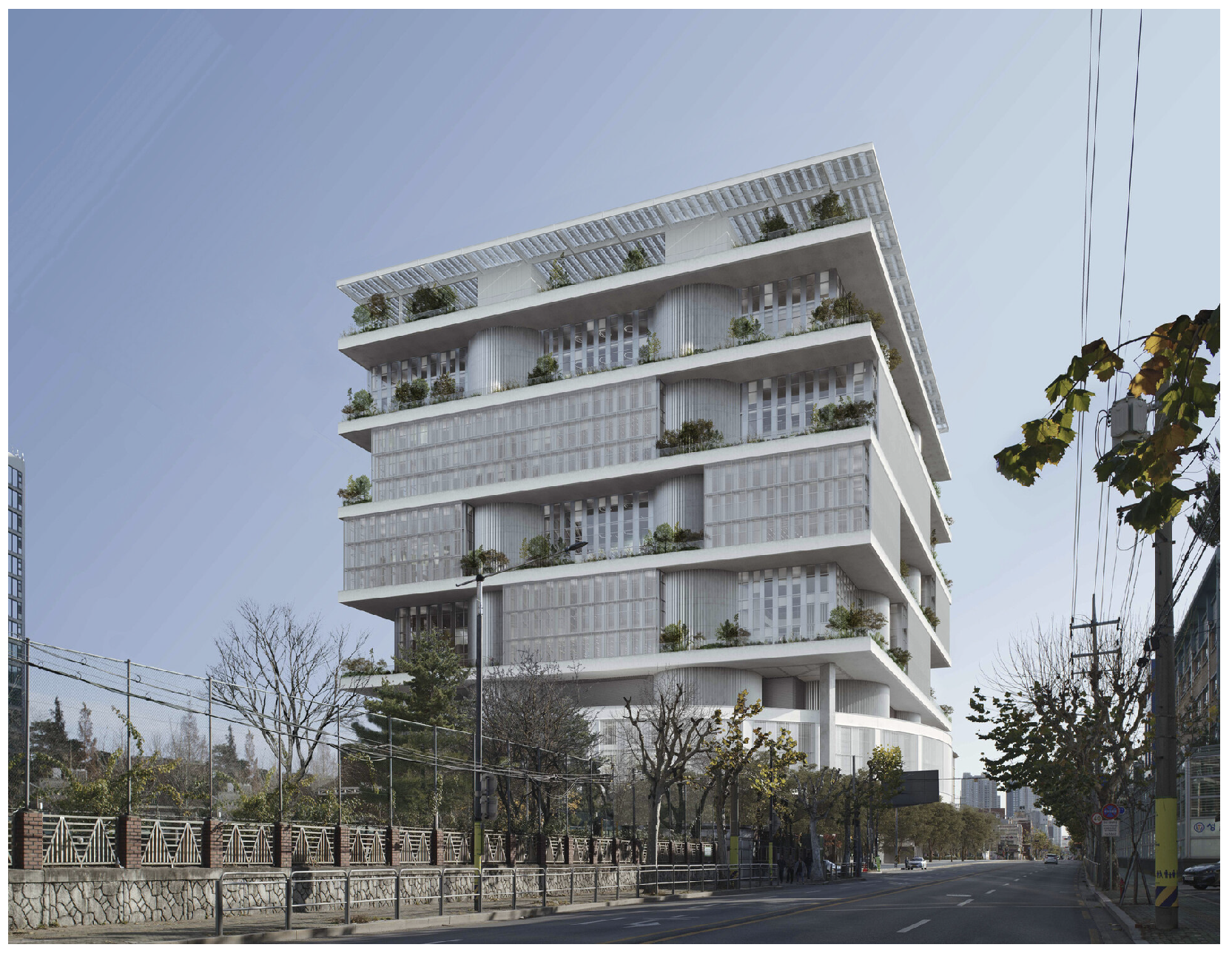
The illustrative case is one typical office floor (5615 m²) of a 17-storey commercial building in Seoul. The case is not a generic example but a project that embodies the central argument of this paper. The flexible floors of the building were initially designed as a full-CLT system—the configuration corresponding to Scenario S2—and the dry zone was subsequently reduced and concentrated within the high-churn central area in response to the practical cost pressures described in Section 1.3, yielding the configuration corresponding to Scenario S3. The S1–S2–S3 comparison developed in this paper therefore traces an actual design trajectory: S2 is the project’s earlier full-CLT ambition, S3 is the hybrid configuration the project has settled on, and S1 is the conventional wet-composite reference against which both are evaluated. The case both motivates the analytical framework and serves as the empirical object on which it is demonstrated (Figure 1).

The building’s occupancy model is the primary driver of reconfiguration frequency. An anchor IT company occupies a core cluster of interconnected levels, with the remaining floors designated as speculative lease space. As the anchor tenant experiences fluctuations in headcount, the resulting programmatic volatility demands localised structural flexibility. During periods of expansion, CLT panels in the central zone are removed to open a vertical void and install an internal staircase connecting adjacent floors. During periods of contraction, those panels are reinstalled to re-close the void, restoring the floor as an independent, leasable unit. Each such open-and-close cycle constitutes one vertical slab-penetration event—the reconfiguration event modelled throughout this study. Treating these openings as reversible rather than as one-off cuts is the project-specific design move that lets the same floor plate absorb successive expansion and contraction cycles over the building’s lifetime.

Architectural logic of the dry zone: The CLT insertion is located along the deep floor area where collaborative space is concentrated—meeting rooms, lounges, hot-desking zones—and where anchor-tenant expansion and contraction cycles trigger internal staircases and voids. Open vertical connections support contemporary headquarters programme requirements by counteracting the communication decay effect of stacked floor plates [16], as in local precedents such as Amorepacific Headquarters in Seoul [17]. Locating the dry zone here means vertical connections can be added and removed with minimal structural carbon cost; the stable perimeter retains wet composite slab, matched to less volatile desk layouts.

This event type cannot be accommodated without structural intervention in a conventional wet composite slab: saw-cutting and breaking out concrete to open the void, and re-casting concrete to close it. In the dry CLT zone, the same spatial change requires only unbolting and reinstalling panels using manual labour and the pre-installed RAPTOR lifting rings (Rothoblaas GmbH, Cortaccia sulla Strada del Vino, Italy), without disturbing the adjacent wet slab. The carbon difference between these two operations—the wet penalty for cutting and re-casting concrete versus the much smaller cost of unbolting and reinstalling a panel—is formalised on the structural slab/panel boundary by the indicators developed in Section 3.6.2, with per-event GWP values derived in Section 3.7.1.

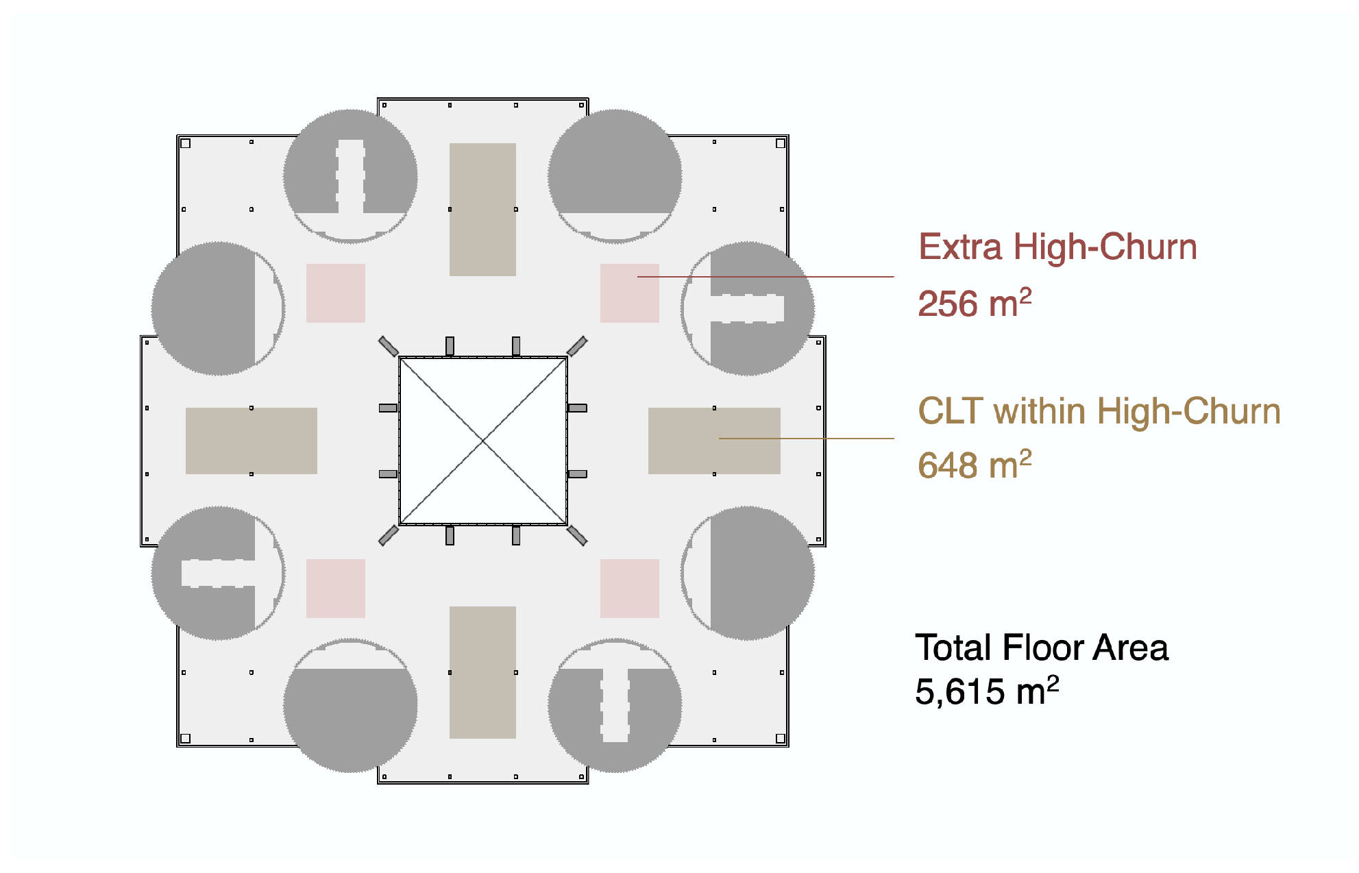
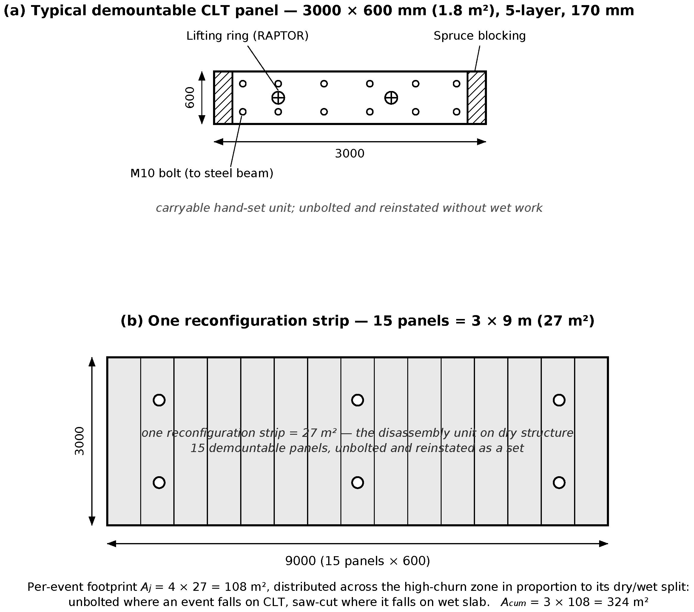
The perimeter zone of the floor supports relatively stable desk-based working activities and is not subject to vertical penetration events; it retains a conventional wet composite slab. The high-churn zone (HCZ)—the bounded sub-area of the floor where the occupancy program concentrates reconfiguration events—covers 904 m² (16.1% of the floor area; Figure 2) and encompasses the deep-plan central collaborative area where anchor tenant expansion/contraction cycles are anticipated to produce slab-penetration events. Of this 904 m², the hybrid strategy places 648 m² of dry CLT construction—four 18 × 9 m dry construction zones (“dry zones”; 162 m² each); each dry zone spans six 3 × 9 m reconfiguration strips (27 m² each), and each strip is in turn assembled from fifteen 3000 × 600 mm demountable CLT panels (1.8 m² each, hand-set with M10 bolts and lifting rings; Figure 3)—within the column bays where the dry zones fit the structural condition cleanly. The remaining 256 m² stays on wet composite slab at four interstitial positions that cannot accommodate a full dry zone. About 71.7% of the high-churn zone is therefore dry CLT, and 28.3% remains wet—a dry fraction $\beta =0.717$, formalised as the central design parameter in Section 3.6.5; Figure 2 illustrates this partial-coverage geometry in full. The carbon implication of these residual wet positions is examined in Section 3.6.5.

3.4. Scenario Definitions

Three scenarios are compared. All share the same number and location of slab-penetration events within the 904 m² high-churn zone; what differs is the structural system that occupies the zone.

• S1 (Wet Baseline). Wet steel–concrete composite slab across the full 5615 m² floor—no CLT.
• S2 (Full CLT). Dry CLT panels across the full 5615 m² floor—the theoretical upper-bound reference.
• S3 (Hybrid). Wet composite slab across 4967 m² with a 648 m² CLT insertion (11.5% of the floor) within the 904 m² high-churn zone—the practical design target.

Quantitative outcomes (mass totals, RCI values, derived ratios) are reported in Section 4 once the indicators have been formalised.

3.5. Floor Assembly Specifications

3.5.1. Scenario 1: Wet Steel–Concrete Composite Slab (Baseline)

Scenario 1 is a conventional wet steel–concrete composite slab: reinforced concrete cast on a re-entrant steel deck, compositely connected to steel beams, acting as a rigid diaphragm over the 5615 m² floor. Major reconfiguration events require saw-cutting, breaking out, and re-casting concrete in the affected zones. The slab-mass comparison uses a structural-only basis: re-entrant steel deck (0.8 mm), normal-weight concrete (150 mm at 2400 kg/m³), and steel reinforcement mesh (

Table 1. Scenario 1 (Wet Baseline) structural slab assembly (slab-mass comparison basis).

Layer	Component	Thickness (mm)	Mass (kg/m2)
Structural	Re-entrant steel deck (0.8 mm)	0.8	6.3
Structural	Concrete (normal weight, 2400 kg/m3)	150	360.0
Structural	Steel reinforcement (mesh)	—	12.0
Total (structural slab only)			378.3

).

3.5.2. Scenario 2: Full Dry CLT Floor (Reference)

Scenario 2 is a full dry CLT floor reference: a 170 mm, 5-layer KLH TL CLT panel (KLH Massivholz GmbH, Austria; or equivalent Stora Enso L5s, Stora Enso Wood Products, Austria/Sweden) installed across the full 5615 m² floor with reversible mechanical fixings. At KLH’s declared density of 470 kg/m³ [18], the panel mass is 79.9 kg/m²—the structural comparison item, directly analogous to the wet composite slab in Scenario 1. Ancillary acoustic, fire, connection, and lifting components (

Table 2. Scenario 2/3 CLT zone assembly. The structural panel row is included in the slab-mass comparison. Ancillary rows are excluded from the structural mass comparison but are described for assembly completeness and may be included in CI if declared in the CI inventory boundary.

Layer	Component	Thick. (mm)	Mass (kg/m2)	Comparison
Structural	5-layer KLH TL CLT panel (470 kg/m3)	170	79.9	Included
Acoustic	Rothoblaas Silent Floor Bytum membrane	6	0.5	Excluded
Acoustic	Rothoblaas Xylofon 50 pads (100 × 100 × 6 mm)	6	0.1	Excluded
Fire/joint	Rothoblaas Fire Stripe Graphite tape (50 × 4 mm)	4	<0.1	Excluded
Sealing	Façade Band UV (60 × 0.32 mm)	0.3	<0.1	Excluded
Connection	M10 bolts + Screw-Ø8@300 (L = 140 mm)	—	0.7	Excluded
Connection	Ø8 × 120 blocking screws at Section E	—	0.1	Excluded
Lifting	Rothoblaas RAPTOR lifting rings (8 per panel)	—	<0.1	Excluded
Total (structural panel only)			79.9	Comparison basis

) are excluded from the structural mass comparison but described for assembly completeness.

3.5.3. Scenario 3: Hybrid Partial-Decoupling Floor

Scenario 3 is a hybrid partial-decoupling floor: wet composite slab over 4967 m² and a dry CLT insertion of 648 m² within the 904 m² high-churn zone, using the same CLT panel and dry build-up as Scenario 2. The dry-zone geometry and panel layout are described in Section 3.3. The wet/dry interface is detailed as a mixed mechanical joint with blocking, sealing (Façade Band UV, Fire Stripe Graphite tape), and CNC-prepared panel geometry; Rothoblaas RAPTOR lifting rings enable panel removal without disturbing adjacent wet slab.

3.5.4. Slab-Mass and CI Inventory Boundary

In line with the system boundary stated in Section 3.2, the slab-mass comparison and the CI calculation use the structural slab/panel basis only: 150 mm wet composite slab for Scenario 1 and 170 mm CLT panel for Scenarios 2 and 3, excluding ancillary dry-system components (acoustic pads, membranes, tapes). The full component inventory and recovery potential assumptions are provided in Appendix C.

3.6. Mathematical Formulation of Key Indicators

The mathematical logic developed below was derived from the illustrative case but applies to any hybrid floor for which a structural slab/panel boundary, an event type, and an occupancy-driven event schedule can be declared. Three primary indicators are used to compare the scenarios: the Circularity Index (CI), the absolute Reconfiguration Global Warming Potential (${\mathrm{GWP}}_{\mathrm{reconf}}$), and the Reconfiguration Carbon Intensity (RCI).

3.6.1. Circularity Index (CI)

The Circularity Index is a mass-weighted per-assembly aggregation of Abu-Ghaida’s product-level Recovery Potential. It is constructed in the building-circularity-indicator tradition [13] to summarise end-of-life recoverability at the assembly scale. For a floor assembly of n components, CI is calculated as:

$$\mathrm{CI}={\displaystyle \frac{{\sum }_{i=1}^n\left(m_i·{\mathrm{RP}}_i\right)}{{\sum }_{i=1}^n{m}_i}}$$

(1)

where $m_i$ is the total mass of component i within the system boundary, and ${\mathrm{RP}}_i$ is the Recovery Potential of component i (ranging from 0 to 1). Recovery Potential is mapped from Disassembly Potential using the material-specific function of Abu-Ghaida et al. [2]:

$${\mathrm{RP}}_i=f\left({\mathrm{DP}}_i\right)$$

(2)

where ${\mathrm{DP}}_i$ is the Disassembly Potential of component i (reflecting connection reversibility, derived from the four-criterion scoring method of [2]; see Appendix C) and $f\left(·\right)$ is the material-specific DP-to-RP mapping reported by Abu-Ghaida et al. DP and RP are adopted directly from [2] without modification.

3.6.2. Reconfiguration Event Definition

A reconfiguration event is defined as a single vertical slab-penetration cycle: the opening of an inter-floor void through the structural slab and its subsequent re-closure. This event type is the focus of the study because it is structural—the slab itself is cut, not only the layers above it—and because it is the event for which the wet/dry distinction produces the largest and most reproducible carbon differential. The per-event GWP for each structural system is derived from the assembly specifications in Section 3.7.1 and Appendix B.

3.6.3. Cumulative Intervention Area ($A_{\mathrm{cum}}$)

Given that the hybrid scenario (S3) experiences highly localized churn rates that differ from the rest of the floor plate, spatial normalization is required. The cumulative intervention area ($A_{\mathrm{cum}}$) quantifies the total physical area affected by reconfiguration over the study period:

$$A_{\mathrm{cum}}={\displaystyle \sum _{j=1}^E}{A}_j$$

(3)

where $A_j$ is the floor area (m²) dismantled and rebuilt during a given reconfiguration event j, and E is the total number of intervention events over the 60-year analysis horizon. The dismantled-and-rebuilt footprint of a single event is taken as 108 m²—the area of four 3 × 9 m reconfiguration strips, each comprising fifteen 3000 × 600 mm demountable CLT panels (27 m²; Figure 3)—so that $A_j=4\times 27=108$ m² per event. The four strips fix the area of the footprint rather than its structural make-up: $A_j$ is an area magnitude set by the reconfiguration programme, and under demand-neutrality (Section 3.2) its location within the high-churn zone follows the zone’s dry/wet composition rather than being confined to the dry construction. Where the footprint falls on dry construction, the panels are unbolted and reinstated to open and re-close a void; where it falls on the wet slab, an equivalent area is saw-cut and re-cast for the same spatial change. The same 108 m² footprint is accordingly costed as entirely saw-cut in the all-wet baseline (S1), entirely unbolted in the full-CLT zone (S2), and—in the hybrid floor, where 71.7% of the high-churn zone is dry—unbolted over that fraction and saw-cut over the remainder, yielding the area-weighted per-event intensity of Equation (6). The per-event footprint $A_j$ is thus held constant across scenarios while its dry/wet split tracks $\beta$; it is distinct from the high-churn zone area $A_z=904$ m², which sets the dry fraction $\beta$ and zone-concentration ratio ${\alpha }_z$ but is not disturbed in its entirety by any single event.

3.6.4. Reconfiguration Carbon Intensity (RCI)

The Reconfiguration Carbon Intensity (RCI) normalises the total reconfiguration GWP against the cumulative intervention area, isolating the carbon efficiency of the structural assembly method from the frequency of tenant-driven change:

$$\mathrm{RCI}={\displaystyle \frac{{\mathrm{GWP}}_{\mathrm{reconf}}}{A_{\mathrm{cum}}}}={\displaystyle \frac{{\sum }_{j=1}^E({\mathrm{GWP}}_{\mathrm{demo},j}+{\mathrm{GWP}}_{\mathrm{prod},j}+{\mathrm{GWP}}_{\mathrm{inst},j})}{A_{\mathrm{cum}}}}$$

(4)

where ${\mathrm{GWP}}_{\mathrm{reconf}}$ is the absolute Reconfiguration GWP (kg CO₂e) summed over all penetration events, and ${\mathrm{GWP}}_{\mathrm{demo},j}$, ${\mathrm{GWP}}_{\mathrm{prod},j}$, ${\mathrm{GWP}}_{\mathrm{inst},j}$ are the demolition, production, and installation GWPs for the structural slab material displaced and replaced during event j. All three components are evaluated on the structural slab/panel boundary defined in Section 3.2. Per-event GWP values for the wet and dry systems are derived in Section 3.7.1.

3.6.5. Parametric Behaviour of RCI for Hybrid Floor Systems

Consider a floor of total area $A_T$ that contains a bounded high-churn zone of area $A_z$. The zone-concentration ratio ${\alpha }_z=A_z/A_T\in (0,1]$ is the high-churn zone’s share of the total floor area. Let $\beta \in [0,1]$ denote the dry fraction—the proportion of the zone constructed as dry, demountable CLT—so that the remaining $(1-\beta )$ stays wet composite. In practice, $\beta <1$ because architectural zones rarely align exactly with the structural grid on which the dry zones are placed. Let $g_w$ and $g_d$ be the per-event reconfiguration GWP per unit area for the wet and dry systems, respectively, with $g_d\ll g_w$ (base-case values $g_w=82.0$ and $g_d=30.4$ kg CO₂e/m², derived in Section 3.7.1 and Appendix A), and let E be the number of events over the study period.

Under demand-neutrality (Section 3.2), E and the per-event footprint $A_j$ are properties of the occupancy program and are identical across scenarios; $\beta$ is the design variable. Events of footprint $A_j$ are distributed across the zone in proportion to its composition, so the expected per-event intensity is the area-weighted average of $g_w$ and $g_d$.

Indicator forms. Two consequences follow from the demand-neutral setup. First, $A_{\mathrm{cum}}$ is invariant with respect to $\beta$:

$$A_{\mathrm{cum}}=E{A}_j$$

(5)

Second, the total reconfiguration GWP is the area-weighted sum across the zone, and the carbon intensity is its per-area normalisation:

$${\mathrm{GWP}}_{\mathrm{reconf}}=E{A}_j\left[(1-\beta )g_w+\beta g_d\right],\mathrm{RCI}\left(\beta \right)={\displaystyle \frac{{\mathrm{GWP}}_{\mathrm{reconf}}}{A_{\mathrm{cum}}}}=(1-\beta )g_w+\beta g_d$$

(6)

The absolute saving of a hybrid with dry fraction $\beta$ relative to the wet baseline is therefore:

$$\Delta {\mathrm{GWP}}_{\mathrm{reconf}}=E{A}_j\beta (g_w-g_d)$$

(7)

Three properties. (i) RCI is a linear blend of $g_w$ and $g_d$ weighted by $\beta$; it is invariant to zone size, event count, and study period—the expected behaviour of a scale-invariant intensity indicator. (ii) Under partial coverage ($\beta <1$), the gap $(1-\beta )(g_w-g_d)$ is the program-to-structure mismatch penalty: the additional reconfiguration carbon incurred because some events land in wet slab within the high-churn zone. (iii) The benefit-to-conversion ratio at the floor-plate level is

$${\displaystyle \frac{\mathrm{benefit}\mathrm{captured}}{\mathrm{conversion}\mathrm{fraction}}}={\displaystyle \frac{\beta }{\beta {\alpha }_z}}={\displaystyle \frac{1}{{\alpha }_z}}$$

(8)

which is independent of $\beta$ and governed solely by how spatially concentrated reconfiguration activity is. The disproportionality of zone-scale reversibility is therefore a function of zone concentration, not of coverage depth. The qualitative result—that localising reversibility in a high-churn zone captures most of the full-decoupling intensity benefit at a fraction of the converted area—follows from the indicator definitions alone and does not depend on specific values of $g_w$, $g_d$, E, or ${\alpha }_z$.

Generalisation when CLT placement diverges from the high-churn zone. The parameter $\beta$ above implicitly assumes all CLT lies inside the HCZ. When a project’s structural grid, service routing, or existing structure prevents this, the proper general parameter is

$${\beta }_{\mathrm{HCZ}}={\displaystyle \frac{A_{\mathrm{CLT}\cap \mathrm{HCZ}}}{A_{\mathrm{HCZ}}}}$$

(9)

i.e., the share of the HCZ that is dry, regardless of any CLT placed outside the HCZ. Equation (6) then reads $\mathrm{RCI}=(1-{\beta }_{\mathrm{HCZ}})g_w+{\beta }_{\mathrm{HCZ}}{g}_d$ unchanged in form. A second area ratio, ${\beta }_{\mathrm{floor}}=A_{\mathrm{CLT}}/A_T$, governs total floor mass and therefore CI. The illustrative case (Section 3.3) corresponds to $\beta ={\beta }_{\mathrm{HCZ}}={\beta }_{\mathrm{floor}}/{\alpha }_z$ because all CLT lies inside the HCZ; the general case allows ${\beta }_{\mathrm{HCZ}}<{\beta }_{\mathrm{floor}}/{\alpha }_z$, with the gap measuring stranded CLT mass that contributes to CI but not to RCI. Empirical behaviour under different placement configurations is examined in Section 4.6.

3.7. Reconfiguration Event Model

LCA modelling assumptions. Biogenic carbon follows the EN 15804+A2 [19] $-1/+1$ characterisation: uptake during forest growth is characterised as $-1$ kg CO₂e per kg CO² within modules A1–A3 and the corresponding re-emission as $+1$ kg CO₂e per kg CO² within module C, irrespective of the end-of-life route. Over a closed cradle-to-grave inventory for sustainably-sourced timber, the two entries cancel, so the net biogenic contribution tends to zero across the 60-year reference study period; EN 15804+A2 additionally prohibits any credit for temporary carbon storage or delayed emissions in the GWP indicators. EN 15804+A2 is adopted in preference to the principal alternatives for three reasons. First, it is the binding core-rules standard for the construction-product EPDs that anchor every per-event intensity in this study (Appendix A), so using its biogenic convention keeps the foreground inventory methodologically consistent with its own data sources rather than mixing accounting rules. Second, the principal alternative standards apply the same underlying $-1/+1$ characterisation and likewise reject temporal-storage credits in the headline metric, so they yield the same near-zero cradle-to-grave net for sustainably-sourced timber—but they differ in how biogenic flows are reported, and the present choice is not equivalent to assuming they are interchangeable. ISO 14067:2018 [20] (clause 6.5.2) mandates the identical $-1/+1$ characterisation but requires biogenic removals and emissions to be documented separately and excludes in-product biogenic carbon content from the reported footprint value (clause 6.4.9); the GHG Protocol Product Standard [21] similarly requires biogenic and non-biogenic flows to be reported separately and excludes weighting factors for delayed emissions. EN 15804+A2 instead publishes biogenic carbon as a named GWP-biogenic sub-indicator of GWP-total. The numerical convergence to a near-zero net is therefore conditional—on closure of the system boundary at end-of-life, sustainable-forestry certification, the absence of significant landfill methane (characterised at its IPCC GWP₁₀₀), and the use of static rather than dynamic characterisation—rather than a property the standards share unconditionally. Third, the static $-1/+1$ characterisation is itself a recognised simplification: a dynamic-LCA treatment in the sense of Levasseur et al. [14] would redistribute the credit and debit in time, and the wider mass timber LCA literature reports that the biogenic-accounting choice can shift building-level GWP materially. In the present study, however, the reported indicators are defined on fossil GWP, so biogenic carbon lies outside the reconfiguration intensity altogether; under EN 15804+A2 it is reported separately as the GWP-biogenic sub-indicator and does not enter the fossil per-event values $g_w$ and $g_d$ on which RCI is computed. The biogenic accounting choice thus affects the absolute presentation of cradle-to-grave carbon but not the reconfiguration carbon differences that this study reports, a limitation revisited in Section 5.3. The per-event reconfiguration GWP on this boundary is dominated by process emissions (cement calcination, primary steel) and fuel-based intercontinental transport, both largely insensitive to electricity-grid decarbonisation; grid intensity is principally a determinant of operational rather than embodied carbon. Only a small, electricity-intensive fraction of each intensity is grid sensitive—electric-arc-furnace reinforcement, galvanizing, and on-site power tools (Appendix A)—and this fraction is the larger for the wet system, which carries the steel and concrete electricity loads. Full decarbonisation of the Korean grid would therefore leave the headline RCI reduction essentially unchanged, and, if anything, move it marginally downward; the per-event intensities $g_w$ and $g_d$ are accordingly treated as static central values, and the prospective shift is second-order on this boundary. Reused materials follow the 100:0 cut-off allocation. Disassembly interdependencies are not modelled explicitly but apply equally across scenarios.

3.7.1. Per-Event GWP: Boundary and Derivation

The per-event GWP per unit area (g, kg CO₂e/m²) is evaluated on the structural slab/panel boundary (Section 3.2) and comprises demolition, production, and installation stages:

$$g={\mathrm{GWP}}_{\mathrm{demo}}+{\mathrm{GWP}}_{\mathrm{prod}}+{\mathrm{GWP}}_{\mathrm{inst}}$$

(10)

The bottom-up derivation of both values from the assembly specifications in Table 1 and Table 2, with full citation of the underlying Korean concrete LCI, KEITI-registered Korean Environmental Product Declarations (EPDs) for rebar and steel deck, European CLT EPDs, and inter-continental CLT transport inventory (Austria/Sweden → Busan → Seoul), is provided in Appendix A. The headline values are S1 (wet composite slab), $g_w=82.0$ kg CO₂e/m² (saw-cutting, breaking out, and re-casting the 150 mm concrete/steel-deck assembly, with concrete A1–A3 anchored on the Korean ready-mix concrete LCI of Choi and Tae [22] cross-checked against the KEITI database mean of $n=1908$ Korean ready-mix EPDs [23], rebar on the Hyundai Steel KEITI-registered EPD [24], steel deck on the POSCO galvanized steel-sheet EPD [25], and demolition/transport on Coelho and de Brito [26]); S2/S3 CLT zone, $g_d=30.4$ kg CO₂e/m² (unbolting the 170 mm CLT panel and reinstalling or replacing, with A1–A3 anchored on the Stora Enso [27], KLH [18], and Binderholz [28] EPDs and the systematic review of Younis and Dodoo [29], transport on Hemmati et al. [30], the Asia–Northern-Europe trade-lane reference of Notteboom et al. [31], and IMO [32], fasteners on the Hilti structural timber screw EPD [33], and acoustic/sealing components on Rothoblaas datasheets [34] with the BMI Icopal SBS-membrane EPD [35]). The dry-case $g_d$ is therefore not a pure unbolt-and-reinstall figure; it assumes approximately 30% panel replacement per cycle to account for edge damage, fastener hole wear, and re-machining of panels disturbed during dismantling, plus full renewal of consumable acoustic and sealing components; the residual ∼70% of panel mass cycles back into the floor through reinstallation. This replacement fraction is an engineering assumption for which no direct empirical measurement exists; it is therefore treated as an explicit scenario variable—varied across low-damage (20%), base (30%), and high-damage (50%) cases in Section 4.4.3—rather than only through the EPD-variation range of $g_d$. The gap $g_w-g_d=51.6$ kg CO₂e/m² per event is the wet coupling penalty.

EPD-vintage note. The deterministic $g_d$ value is anchored on the KLH [18], Stora Enso [27], and Binderholz 2019 IBU [28] EPDs. A 2024 MRPI successor for the Binderholz CLT BBS product [36] became available during manuscript preparation but is not used here; its A1–A3 ${\mathrm{GWP}}_{\mathrm{fossil}}$ values fall within the OAT envelope of Section 4.4, so re-deriving against it would not change the 45.1% headline.

3.7.2. Event Frequency and Cumulative Intervention Area

Three vertical slab-penetration events are assumed over the 60-year study period within the 904 m² high-churn zone (one cycle approximately every 20 years). No published Korean dataset quantifies slab-penetration cadence directly; the assumed frequency is inferred from three related empirical sources. Cho and Choi [37] documented 5-year minimum lease structures in all 19 TI-paying Seoul Prime office buildings they surveyed in 2016 Q4, establishing the basic lease-cycle anchor. Forsythe [38] measured an 8.2–8.5-year fit-out churn rate in 528 Sydney CBD Prime buildings, providing the closest Anglophone comparator; no Asian-market replication exists. Cho and Choi [39] found 25–30-year major remodelling cycles for Seoul Grade B+ offices, bounding the upper end of structurally-disruptive intervention frequency. Combining these, slab penetrations are assumed to occur at approximately one-third the frequency of non-structural fit-out cycles, yielding 2–6 events over 60 years with a mode near 3; a 6-event upper bound is additionally tested in Section 4.4 as a stress case representing tenancy programmes with accelerated reconfiguration cadences beyond the inferred empirical envelope. The three-event cadence is therefore presented as a scenario assumption inferred from related leasing- and fit-out-cycle proxies, not as a directly measured slab-penetration frequency; the 2- and 6-event variants accordingly bracket it as a scenario range rather than as confidence bounds on a measured quantity.

Under demand neutrality (Section 3.2), event count and event location are held constant across all three scenarios. Each event disturbs a per-event footprint of $A_j=108$ m² (the area of four 27 m² reconfiguration strips; Section 3.6.3), placed across the high-churn zone in proportion to its composition, so $A_{\mathrm{cum}}=3\times 108=324$ m² for all scenarios. Sensitivity to event count is examined in Section 4.4 with bounding cases of 2 (low) and 6 (high). Non-structural fit-out, service, and finish cycles occur at their own cadences but do not penetrate the structural slab and fall outside the RCI boundary.

4. Results

The results are presented on a whole-to-part progression: The structural slab mass that each scenario commits (Section 4.1) establishes the material basis of the comparison; the reconfiguration carbon intensity (Section 4.2) is the central use-phase indicator derived from it; the absolute reconfiguration GWP places that intensity in absolute terms on a common intervention footprint; and the combined circularity–RCI plane positions the scenarios jointly on both indicators. Establishing the material substitution before the indicators derived from it lets each carbon result be read in light of the physical change that produces it.

4.1. Slab Mass Comparison

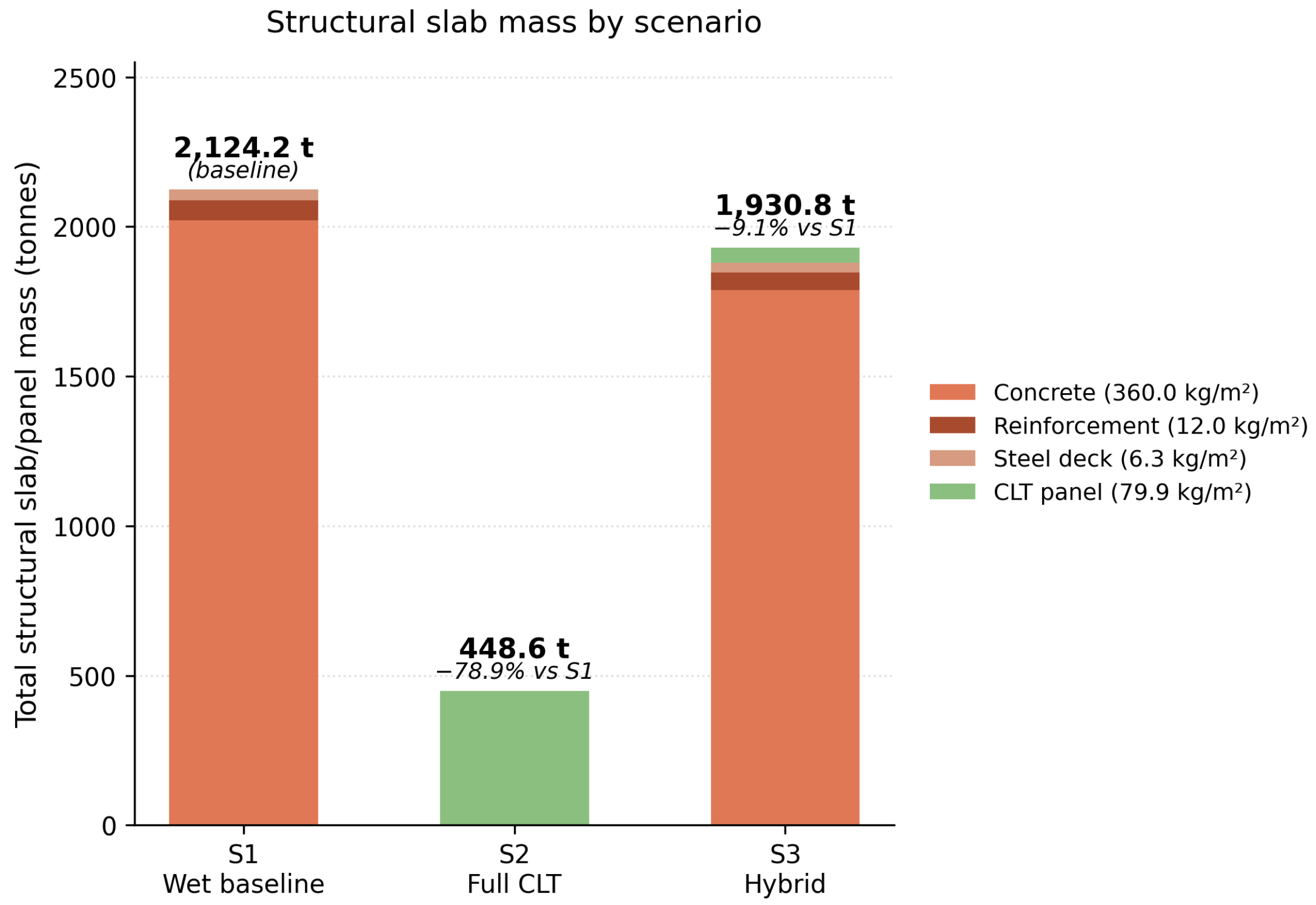
Figure 4 shows the total slab mass breakdown for each scenario on a structural slab/panel-only basis. The hybrid strategy (S3) achieves a 9.1% mass reduction relative to the wet baseline (S1) by replacing 648 m² of wet composite slab (378.3 kg/m²) with 170 mm CLT panel (79.9 kg/m²), saving 193.4 t of structural slab mass. The full CLT scenario (S2) achieves a 78.9% mass reduction. The internal component annotation in Figure 4 reflects the structural-only breakdown of Table 1.

4.2. Reconfiguration Carbon Intensity and Cumulative GWP

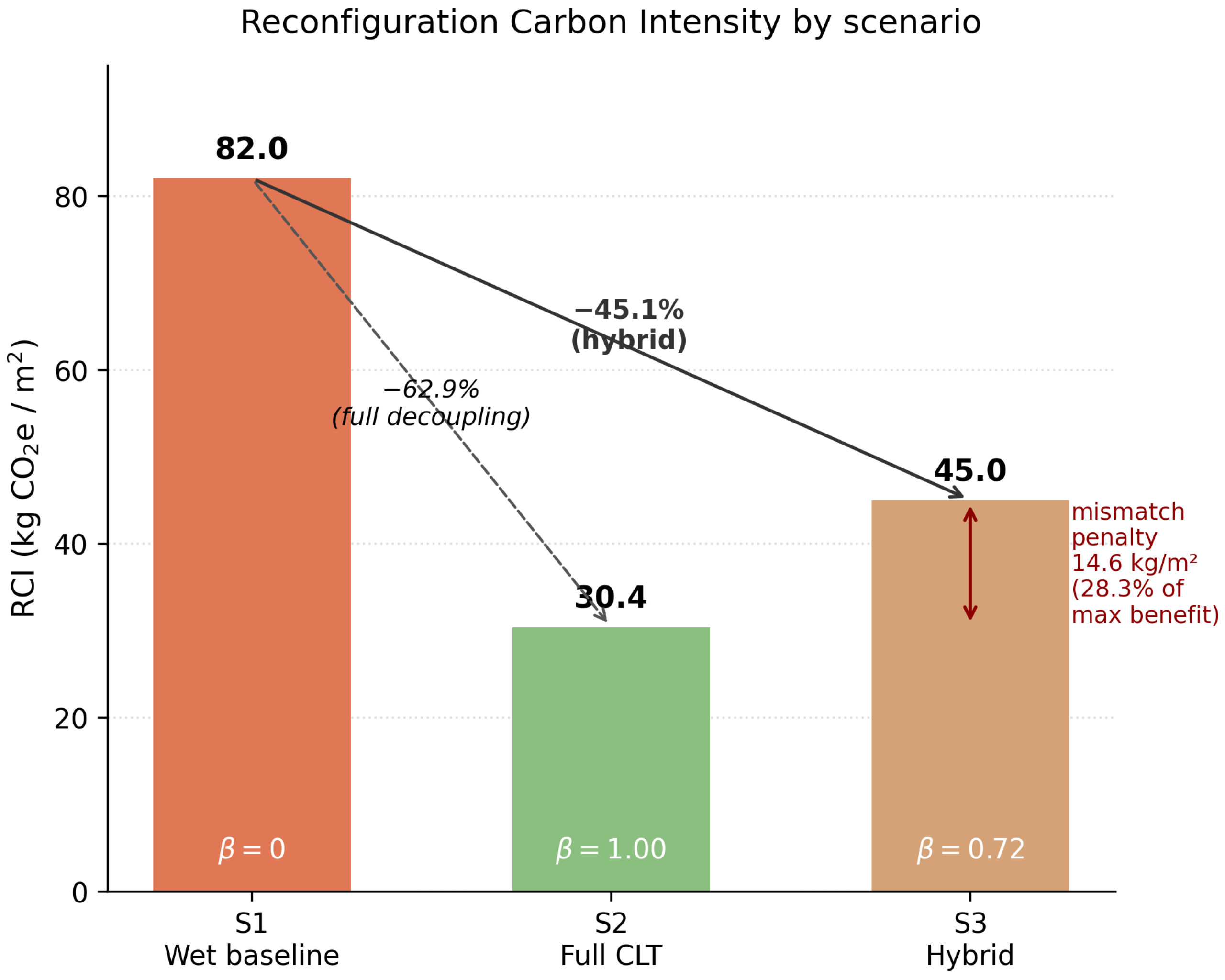
Figure 5 reports the reconfiguration carbon intensity (RCI) for each scenario: ${\mathrm{RCI}}_{\mathrm{S}1}=82.0$, ${\mathrm{RCI}}_{\mathrm{S}2}=30.4$, and ${\mathrm{RCI}}_{\mathrm{S}3}=45.0$ kg CO₂e/m². The hybrid reduces RCI by 45.1% relative to the wet baseline, capturing 71.7% of the 62.9% reduction achievable by full decoupling. By Equation (6), ${\mathrm{RCI}}_{\mathrm{S}3}=(1-0.717)\left(82.0\right)+\left(0.717\right)\left(30.4\right)=45.0$, matching the zone-averaged intensity expected for $\beta =0.717$. The 28.3% shortfall is the program-to-structure mismatch penalty $(1-\beta )(g_w-g_d)=14.6$ kg CO₂e/m² derived in Section 3.6.5; the hybrid converts only 11.5% of the total floor area to CLT while delivering this benefit, giving a benefit-to-conversion ratio of $6.2\times$. That is, the share of the use-phase intensity benefit captured (71.7%) is 6.2 times the share of the floor area converted to dry construction (11.5%); this ratio equals $1/{\alpha }_z$ with ${\alpha }_z=0.161$.

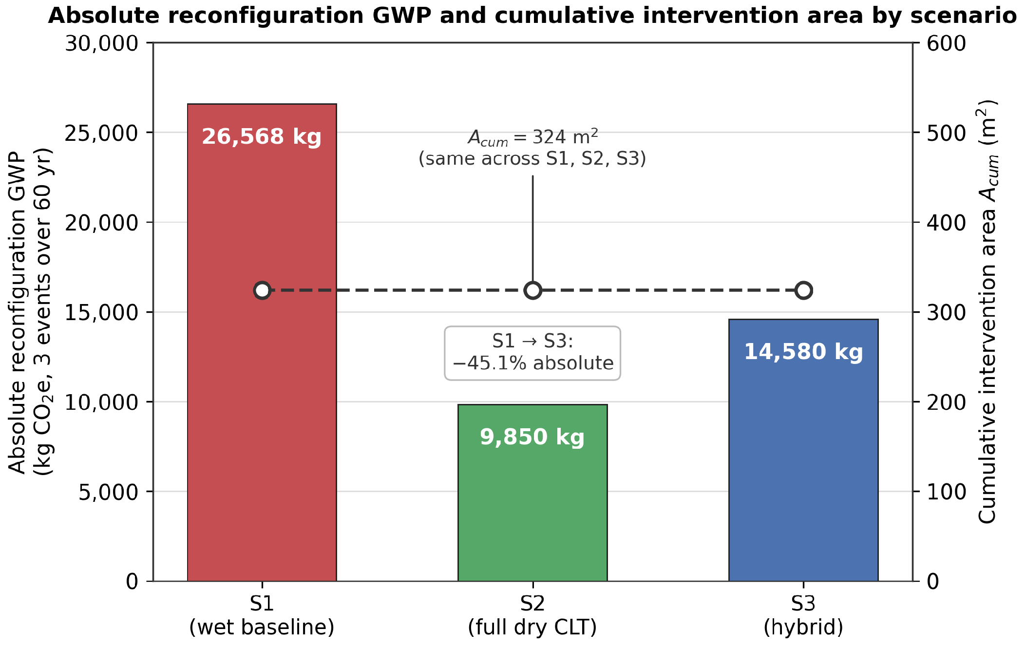
Figure 6 presents the absolute reconfiguration GWP and cumulative intervention area. As all three scenarios share the same three penetration events with the same per-event footprint ($A_j=108$ m²), $A_{\mathrm{cum}}$ is identical across them at 324 m². The absolute reconfiguration GWP is 26,568 kg CO₂e for S1, 9850 kg for S2, and 14,580 kg for S3 (detailed arithmetic in Appendix B). The hybrid therefore reduces absolute reconfiguration GWP by 45.1%, consistent with the RCI result and with equal $A_{\mathrm{cum}}$ across scenarios.

4.3. Circularity Index vs. Reconfiguration Carbon Intensity

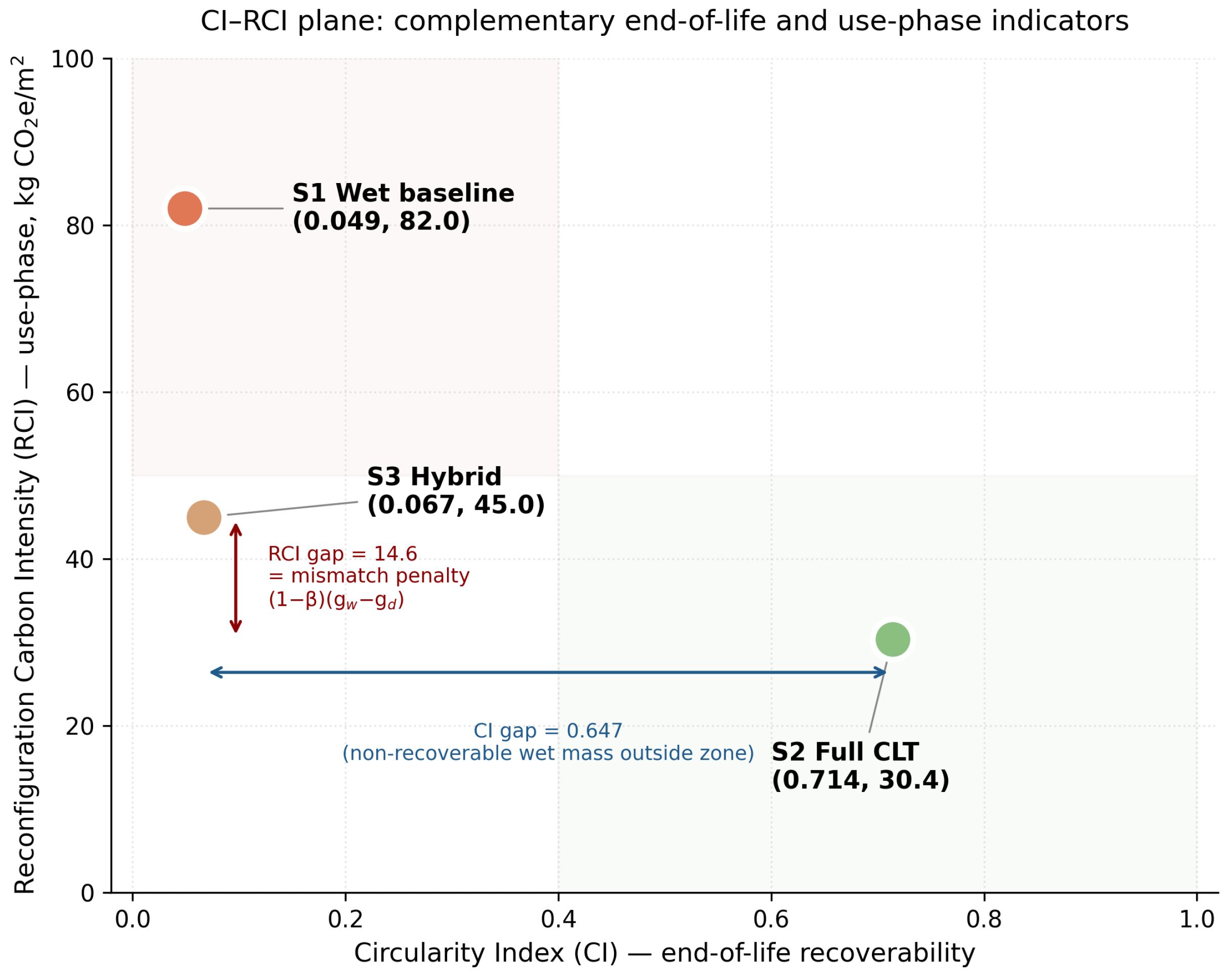
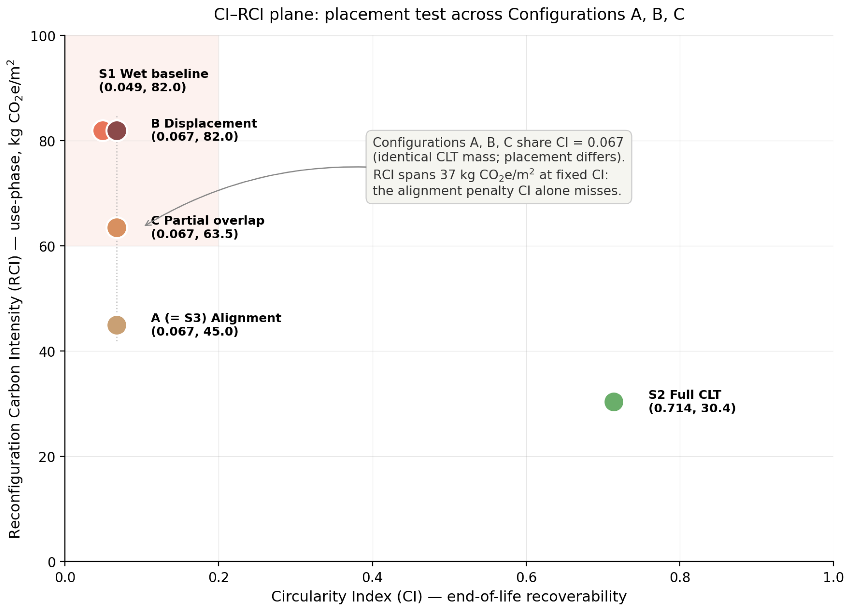
Figure 7 maps all three scenarios on a CI–RCI plane. S1 sits in the low-CI, high-RCI region ($\mathrm{CI}=0.049$, $\mathrm{RCI}=82.0$); S2 in the high-CI, low-RCI region ($\mathrm{CI}=0.714$, $\mathrm{RCI}=30.4$); S3 between them at intermediate values ($\mathrm{CI}=0.067$, $\mathrm{RCI}=45.0$). S3 captures 71.7% of the use-phase intensity benefit and 3% of the end-of-life recoverability benefit relative to S1 while converting only 11.5% of the floor area. The two indicators are separable on both axes; design implications are interpreted in Section 5.1.

4.4. Sensitivity Analysis

Under the demand-neutral, structural-only event model, RCI depends on the per-event GWP inputs ($g_w$, $g_d$) and on the dry fraction $\beta$ of the high-churn zone (see Equation (6)); it is invariant to event count, zone size, and study period. Absolute reconfiguration GWP saving, by contrast, scales with $\beta$, per-event footprint, event count, study period, and the gap $(g_w-g_d)$ (see Equation (7)). Parameters fall into two groups (

Table 3. Sensitivity analysis parameters and tested ranges. Both = changes RCI and absolute GWP saving; Scale = changes absolute GWP saving only. The $\beta$ values are treated as a continuous design-space sweep; physically realisable discrete configurations within the 904 m² HCZ correspond to whole-zone counts ($\beta \in \{0,0.179,0.358,0.538,0.717,0.896\}$ for 0–5 dry zones of 162 m² each), with $\beta =0.358$ examined as Configuration C in Section 4.6; $g_w$, $g_d$ ranges span $\pm 15$–$25\%$ of base values (plausible EPD variation); the per-event footprint range spans two to eight 27 m² reconfiguration strips around the four-strip base ($A_j=108$ m²).

Parameter	Low/Base/High	Acts on
Dry fraction of zone ($\beta$)	0.50/0.717/1.00	Both
Wet per-event GWP ($g_w$, kg CO2e/m2)	70/82.0/95	Both
Dry per-event GWP ($g_d$, kg CO2e/m2)	25/30.4/38	Both
Per-event footprint ($A_j$, m2)	54/108/216 (2/4/8 strips)	Scale
Event count (E, over 60 yr)	2/3/6	Scale
Study period (yr)	40/60/80	Scale

): scale-only ($A_j$, E, study period) and dual-acting ($g_w$, $g_d$, $\beta$). Within the dual-acting group, $\beta$ is distinct because it is the only parameter set by architectural design rather than by material EPD or occupancy programme.

4.4.1. One-at-a-Time Results

Table 4. Sensitivity analysis results: RCI reduction (%) and absolute GWP saving (million kg CO₂e) for the hybrid relative to the wet baseline.

Parameter	Variant	Value	RCI Red. (%)	GWP Saving (M kg)
Dual-acting parameter (design variable)
$\beta$ (dry fraction)	Low	0.50	31.5	0.008
	Base	0.717	45.1	0.012
	High	1.00	62.9	0.017
Dual-acting parameters (material EPD inputs)
$g_w$	Low	70 kg/m2	40.6	0.009
	Base	82.0 kg/m2	45.1	0.012
	High	95 kg/m2	48.7	0.015
$g_d$	Low	25 kg/m2	49.8	0.013
	Base	30.4 kg/m2	45.1	0.012
	High	38 kg/m2	38.5	0.010
Scale-only parameters (RCI invariant)
Footprint $A_j$	Low	54 m2 (2 strips)	45.1	0.006
	Base	108 m2 (4 strips)	45.1	0.012
	High	216 m2 (8 strips)	45.1	0.024
Event count E	Low	2 events	45.1	0.008
	Base	3 events	45.1	0.012
	High	6 events	45.1	0.024
Study period	Low	40 yr (2 events †)	45.1	0.008
	Base	60 yr (3 events)	45.1	0.012
	High	80 yr (4 events)	45.1	0.016

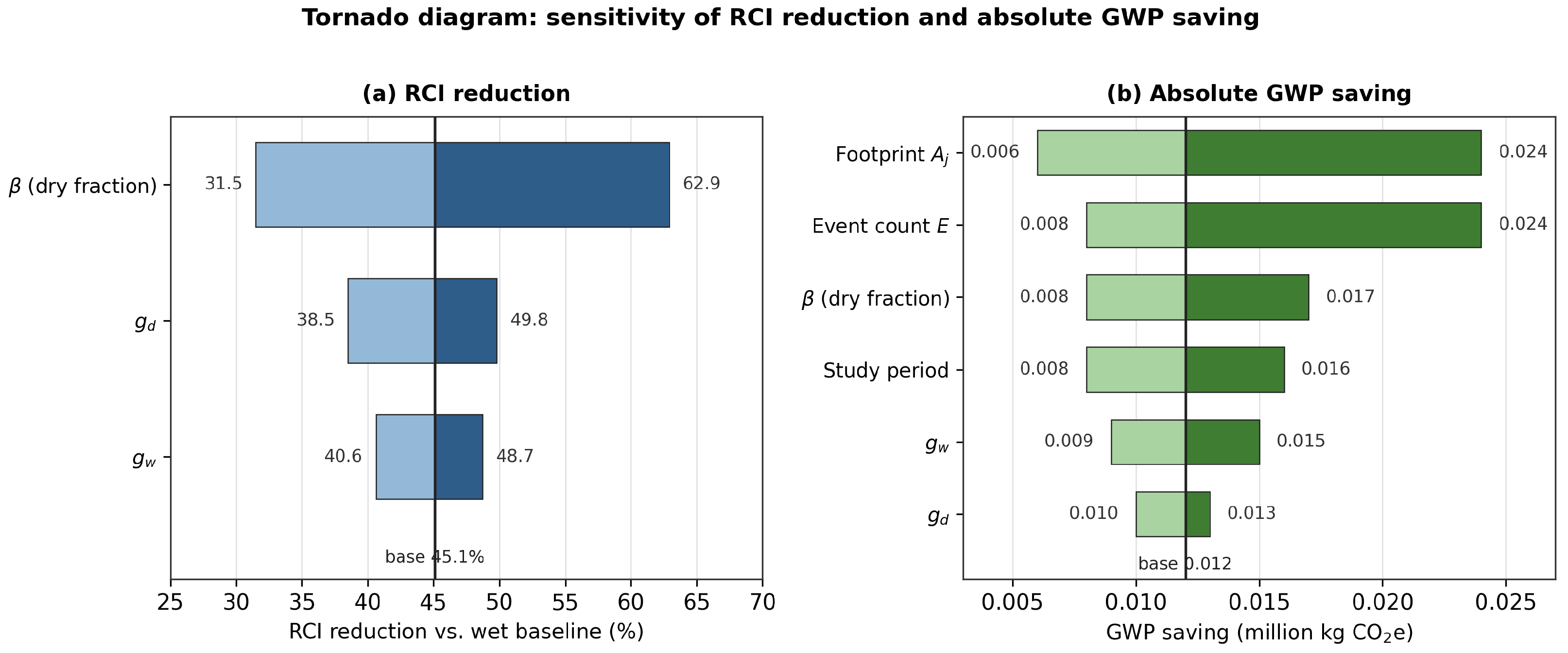
^† Event count scales with study period at one event per 20 years.

presents OAT sensitivity results. Base-case values are ${\mathrm{RCI}}_{\mathrm{S}1}=82.0$, ${\mathrm{RCI}}_{\mathrm{S}3}=45.0$ kg CO₂e/m² (45.1% reduction) and absolute GWP saving = 0.012 million kg CO₂e (26,568 − 14,580). Figure 8 presents the results as a tornado diagram, with dual-acting parameters grouped separately from scale-only parameters.

4.4.2. Interpretation and Robustness

The OAT results align with the analytical predictions of Section 3.6.5. The dry fraction $\beta$ dominates RCI sensitivity (31.5–62.9% across the tested range), reflecting its role as the design lever in $\mathrm{RCI}\left(\beta \right)=(1-\beta )g_w+\beta g_d$. Sensitivity to $g_d$ exceeds that of $g_w$ at base-case $\beta =0.717$ (the partial-derivative weights $\beta$ and $1-\beta$ from Equation (6)), so CLT-EPD improvements compound more strongly than wet-slab-EPD improvements. Scale-only parameters ($A_j$, E, study period) leave RCI reduction at 45.1% by construction and act only on absolute saving. The minimum RCI reduction across all 18 tested variants is 31.5% ($\beta =0.50$); excluding the $\beta$ variants, it is 38.5% (high $g_d$). The hybrid strategy is robust to the principal sources of parametric uncertainty in this analysis.

4.4.3. Damage-Scenario Sensitivity: Panel Replacement Fraction

The dry-case intensity $g_d$ depends on the fraction $\phi$ of CLT panel mass replaced per reconfiguration cycle—a function of edge damage, fastener-hole wear, and re-machining of disturbed panels—for which no direct empirical measurement exists (Appendix A.2). To treat this assumption explicitly rather than only through the EPD-variation range of $g_d$, $\phi$ is varied across three damage scenarios anchored on the bottom-up derivation: a low-damage case ($\phi =0.20$, $g_d\approx 25$), the base case ($\phi =0.30$, $g_d=30.4$), and a high-damage case ($\phi =0.50$, $g_d\approx 46$). The high-damage value deliberately exceeds the EPD-variation OAT high bound ($g_d=38$ kg CO₂e/m²) and is included as a conservative stress case.

Table 5. Damage-scenario sensitivity: hybrid (S3) RCI reduction relative to the wet baseline (S1) as the CLT panel replacement fraction $\phi$ varies, evaluated at base dry fraction $\beta =0.717$ and $g_w=82.0$ kg CO₂e/m². The high-damage case exceeds the EPD-variation OAT bound and is included as a conservative stress scenario; $g_d$ values are anchored on the bottom-up derivation in Appendix A.2.

Scenario	Replacement Fraction $\mathit{\phi }$	${\mathit{g}}_{\mathit{d}}$ (kg CO2e/m2)	RCIS3	RCI Red. vs. S1
Low damage	0.20	∼25	41.1	49.8%
Base	0.30	30.4	45.0	45.1%
High damage	0.50	∼46	56.2	31.5%

reports the resulting RCI reduction at the base dry fraction $\beta =0.717$.

The hybrid retains a substantial use-phase advantage across the entire range: Even under 50% panel replacement per cycle—a high-damage assumption above the plausible EPD envelope—S3 reduces RCI by 31.5% relative to the wet baseline. The conclusion that zone-scale decoupling delivers a material reconfiguration-carbon benefit is therefore robust to the panel-replacement assumption, which is the single most load-bearing input in the $g_d$ derivation.

4.5. Joint Uncertainty and Robustness Checks

The closed-form decomposition (Section 3.6.5) establishes RCI’s structural dependence on ${\beta }_{\mathrm{HCZ}}$, $g_w$, and $g_d$ analytically; the OAT analysis (Section 4.4.1) confirms the marginal hierarchy. This section reports a compact joint-uncertainty stress test and two extensions—a correlation-structure check and an induced-demand breakeven—that sample interactions and assumption-relaxations the OAT cannot supply by construction. The stress test is anchored on Configuration A (CLT placed inside the HCZ, so $\beta ={\beta }_{\mathrm{HCZ}}$); the orthogonal axis of CLT placement relative to the HCZ is treated deterministically in Section 4.6 because it is a design choice rather than a stochastic parameter.

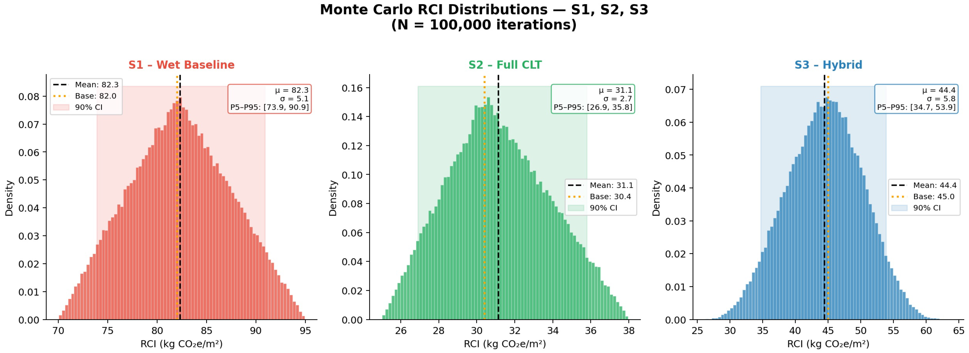
Joint sampling and headline result: A Monte Carlo simulation samples all five parameters simultaneously across the OAT envelope of Table 3. Triangular distributions are used for $g_w$, $g_d$, and ${\beta }_{\mathrm{HCZ}}$ because the endpoints represent hard physical or design bounds; E is a discrete weighted distribution with the base case at $P=0.50$; $A_z$ is truncated normal ($\mu =904$ m², $\sigma =150$ m², approximately $\pm 1$ structural bay). The ${\beta }_{\mathrm{HCZ}}$ range [0.50, 1.00] reflects the alignment configurations achievable when dry zones fit inside the HCZ; placements outside this range correspond to Configurations B and C and are examined separately in Section 4.6. EPD anchors for $g_w$ are the Korean ready-mix concrete compilation of Choi and Tae [22] (1$\sigma \approx 15\%$) together with KEITI/Hyundai Steel rebar references; for $g_d$, the Stora Enso [27], Binderholz [28], and KLH [18] EPDs (modules A1–A3, fossil-only GWP-GHG; no Korean CLT EPD is currently available). The full distribution specification is summarised in

Table 6. Monte Carlo input distributions. Triangular bounds are anchored on the OAT envelope of Table 3; the discrete probability vector for E assigns the dominant mass to the documented base cadence and splits the remainder symmetrically over the lower and higher alternatives; the truncated normal for $A_z$ uses $\sigma$ corresponding to approximately one structural bay. The study period is held fixed at 60 yr because RCI is intensity-normalised and therefore invariant to it. EPD anchors are described in the preceding paragraph.

Parameter	Distribution
${\beta }_{\mathrm{HCZ}}$ (within-HCZ dry fraction)	Triangular$(0.50,0.717,1.00)$
$g_w$ (kg CO2e/m2)	Triangular$(70,82.0,95)$
$g_d$ (kg CO2e/m2)	Triangular$(25,30.4,38)$
$A_z$ (m2)	Truncated normal, $\mu =904$, $\sigma =150$, support $[600,1200]$
E (events over 60 yr)	Discrete: $P\left(2\right)=0.25$, $P\left(3\right)=0.50$, $P\left(6\right)=0.25$

.

Figure 9 shows the resulting RCI distributions, and

Table 7. Monte Carlo summary statistics. Means and medians lie within about one unit of the deterministic base case (the medians closer than the means); P5–P95 intervals give the central 90% of the joint-uncertainty envelope.

Metric	Mean	Median	Std. Dev.	P5	P95	Base
${\mathrm{RCI}}_{\mathrm{S}1}$ (kg CO2e/m2)	82.3	82.3	5.1	73.9	90.9	82.0
${\mathrm{RCI}}_{\mathrm{S}2}$ (kg CO2e/m2)	31.1	31.0	2.7	26.9	35.8	30.4
${\mathrm{RCI}}_{\mathrm{S}3}$ (kg CO2e/m2)	44.4	44.6	5.8	34.7	53.9	45.0
RCI reduction S3 vs. S1 (%)	45.9	45.6	7.0	34.8	58.1	45.1
Benefit-to-conversion ratio (×)	6.4	6.2	1.1	4.9	8.5	6.2

reports the headline metrics. The S1 and S3 distributions do not overlap; the deterministic base-case values lie close to the sample means and medians—within about 1 kg CO₂e/m² for the RCI values and 0.8 percentage points for the reduction, with all base values well inside the P5–P95 envelope; the small offsets reflect the rightward skew of the triangular inputs, whose means sit slightly above their modal base values, and Spearman rank correlations confirm the analytical hierarchy (${\beta }_{\mathrm{HCZ}}$: $\rho =-0.91$; $g_d$: $+0.32$; $g_w$: $+0.23$; $A_z$ and E: $\left|\rho \right|<0.01$, reconfirming RCI’s scale-invariance). The deterministic headlines therefore represent central tendencies rather than optimistic point choices.

Correlation structure. Independent sampling of $g_w$ and $g_d$ is physically implausible because shared background processes (grid electricity, transport, cement clinker factor) couple wet and dry EPDs. Under a Gaussian copula with $\rho (g_w,g_d)=+0.6$, a first-order variance approximation yields

$$\mathrm{Var}\left({\mathrm{RCI}}_{\mathrm{S}3}\right)\approx {(1-{\beta }_{\mathrm{HCZ}})}^2{\sigma }_{g_w}^2+{\beta }_{\mathrm{HCZ}}^2{\sigma }_{g_d}^2+2{\beta }_{\mathrm{HCZ}}(1-{\beta }_{\mathrm{HCZ}}){\rho }_{g_w{g}_d}{\sigma }_{g_w}{\sigma }_{g_d}.$$

(11)

The cross-term raises the variance of ${\mathrm{RCI}}_{\mathrm{S}3}$ itself, but the variance of the reduction ratio $({\mathrm{RCI}}_{\mathrm{S}1}-{\mathrm{RCI}}_{\mathrm{S}3})/{\mathrm{RCI}}_{\mathrm{S}1}$ falls, because that quantity depends on the gap $(g_w-g_d)$ whose variance shrinks under positive correlation. The independent-sampling P5–P95 interval of [34.8%, 58.1%] is therefore a conservative envelope: Realistic correlation structures narrow rather than widen it.

Induced demand and breakeven. Demand-neutrality (Section 3.2) assumes that E is set by the occupancy program and unaffected by reconfiguration cost. If dry reconfiguration is cheaper and less disruptive, tenants plausibly request more of it. Modelling this as $E\left({\beta }_{\mathrm{HCZ}}\right)=E_0(1+k{\beta }_{\mathrm{HCZ}})$ with $E_0=3$ and rebound coefficient $k\ge 0$, RCI reduction remains invariant to E; rebound acts entirely on absolute reconfiguration GWP. Setting ${\mathrm{GWP}}_{\mathrm{S}3}\left(k^{*}\right)={\mathrm{GWP}}_{\mathrm{S}1}$ and cancelling the common factor $E_0{A}_j$ gives the closed-form breakeven

$$k^{*}={\displaystyle \frac{g_w-g_d}{g_w-{\beta }_{\mathrm{HCZ}}(g_w-g_d)}}$$

(12)

valid for ${\beta }_{\mathrm{HCZ}}>0$. At base case (${\beta }_{\mathrm{HCZ}}=0.717$, $g_w=82.0$, $g_d=30.4$ kg CO₂e/m²), $k^{*}=1.15$; the hybrid breaks even only when the rebound coefficient reaches this value, corresponding to an event-count rise of approximately 82% above the wet-baseline cadence ($E_0(1+k^{*}{\beta }_{\mathrm{HCZ}})=1.82E_0$). Rebound tolerance rises with ${\beta }_{\mathrm{HCZ}}$ and falls as the wet–dry gap narrows; because that gap is dominated by process and transport emissions (Section 3.7), it is stable, and $k^{*}$ stays near its base value. No empirical estimate of slab-penetration rebound exists, so $k^{*}$ is presented as an analytical bound rather than a likelihood claim: The hybrid’s absolute-GWP advantage compresses but does not reverse for any rebound coefficient $k<k^{*}$. The lowest tolerances arise in the low-${\beta }_{\mathrm{HCZ}}$ regime already identified as high-mismatch.

4.6. Generalisation: Indicator Behaviour Under Alternative CLT Placements

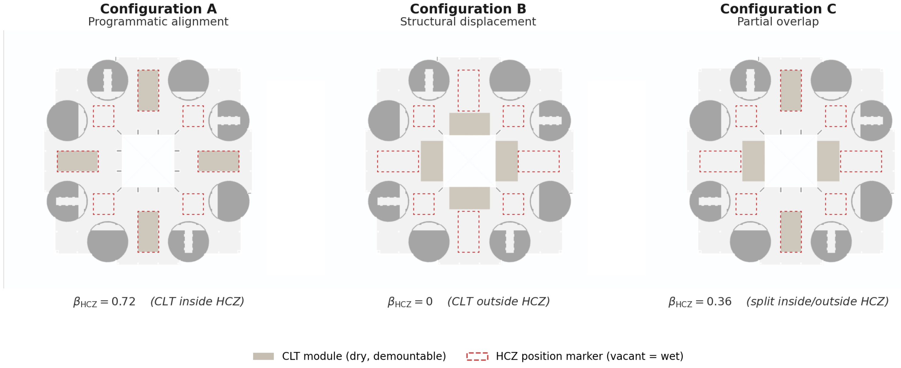
The S1–S2–S3 comparison demonstrates the indicators on the documented design trajectory of one building, in which architectural intent (CLT in the high-churn zone) and structural condition (a column grid that accepts dry zones in that area) coordinated. In real projects this coordination is not guaranteed; column grids, service routing, fire-compartment boundaries, and existing structure can dictate where dry construction is feasible, sometimes far from where reconfiguration events are demanded. Three placement configurations of the same 5615 m² floor are evaluated using the generalised parameter ${\beta }_{\mathrm{HCZ}}$ defined in Section 3.6.5 (see Equation (9)). All three hold CLT quantity (648 m², four dry zones), HCZ (904 m² at the centre), and total floor mass fixed; only CLT placement differs. The discrete, panel-resolved nature of these placements is grounded in the project’s demountable-panel geometry (Figure 3); reconfiguration events open and re-close voids by unbolting whole 3 × 9 m strips, so whether a given event lands on dry or wet structure is set by where the dry zones sit relative to the high-churn zone—the discrete design decision isolated by the configurations below, rather than a randomly distributed area. Where the dry zones only partly coincide with the HCZ (Configuration C below), the events demanded within the HCZ are taken to sample its dry/wet composition in proportion to area, so that the expected per-event intensity is the area-weighted blend $(1-{\beta }_{\mathrm{HCZ}})g_w+{\beta }_{\mathrm{HCZ}}{g}_d$ of Equation (6); this is the same demand-neutral assumption applied to the S3 floor, now resolved within the zone. The three configurations are shown in Figure 10.

• Configuration A—Programmatic alignment (=S3). All four dry zones fall inside the HCZ; ${\beta }_{\mathrm{HCZ}}=0.717$. The grid cooperates with the program; this is the design ideal demonstrated above.
• Configuration B—Structural displacement. The grid does not accept dry zones within the HCZ; the same four dry zones are relocated to a structurally feasible area outside the HCZ; ${\beta }_{\mathrm{HCZ}}=0$. CLT is on the floor but not where events occur. The configuration is retained as a limit case because pinning ${\beta }_{\mathrm{HCZ}}=0$ at fixed CI isolates the indicator’s response to placement, which is the diagnostic point.
• Configuration C—Partial overlap. Two dry zones fall inside the HCZ and two lie outside; ${\beta }_{\mathrm{HCZ}}=0.358$. The realistic intermediate case.

Table 8. Indicator values across the three placement configurations, with S1 and S2 included for reference. Configurations A–C share identical CLT quantity and identical floor mass, so CI is invariant across them while RCI varies with placement.

Case	Description	${\mathit{\beta }}_{\mathbf{HCZ}}$	${\mathit{\beta }}_{\mathbf{floor}}$	CI	RCI (kg CO2e/m2)	RCI Red. (%)
S1	Wet baseline	—	0	0.049	82.0	0
S2	Full CLT	1.00	1.00	0.714	30.4	62.9
A (=S3)	Alignment	0.717	0.115	0.067	45.0	45.1
B	Displacement	0	0.115	0.067	82.0	0
C	Partial overlap	0.358	0.115	0.067	63.5	22.6

reports the indicator values. CI is identical across A, B, and C ($\mathrm{CI}=0.067$) because total floor mass and component composition are identical. RCI separates them across the full reduction range: A captures 45.1% of the wet-baseline intensity benefit; B captures none of it (RCI matches S1 exactly because no event lands on dry surface); C captures 22.6%. Configurations indistinguishable on mass-circularity grounds therefore differ by 0–45 percentage points on use-phase reconfiguration intensity.

Figure 11 maps the five cases on the CI–RCI plane. Configurations A, B, and C all collapse to a single point on the CI axis ($\mathrm{CI}=0.067$) but spread across 37 kg CO₂e/m² on the RCI axis. Configuration C’s intermediate value follows directly from ${\beta }_{\mathrm{HCZ}}=0.358$ via the generalised RCI expression (Section 3.6.5), confirming that the alignment penalty is a continuum rather than a binary.

The placement comparison preserves demand-neutrality; all three configurations assume the same occupancy program demanding the same events in the same HCZ. What changes between configurations is whether the structural system at the demanded location is dry or wet—i.e., whether the building can absorb the demanded events reversibly. The interpretive consequences of this separation are taken up in Section 5.1.

5. Discussion

5.1. CI–RCI Divergence and Its Policy Implication

The placement comparison in Section 4.6 makes the CI–RCI divergence concrete. Configurations A, B, and C share identical mass and identical CI yet span the full 0–45% range of RCI reduction. CI rewards recoverable mass wherever it sits; RCI rewards only the material that actually receives reconfiguration events. The two indicators are not redundant statements of the same underlying property—they answer different questions about the same physical boundary, and on hybrid floors they can disagree across the full reduction range.

The policy implication is direct. Frameworks that rely solely on mass-weighted end-of-life circularity rank Configuration B equivalent to Configuration A despite delivering no use-phase reconfiguration benefit, and may discourage well-aligned hybrid strategies relative to displaced ones if mass alone is the metric. Pairing CI with RCI, on a shared structural boundary, exposes this asymmetry and lets hybrid floors be evaluated on what they actually do during the use phase rather than only on what is recoverable at end-of-life.

The framework also generalises to any reconfigurable building element where two construction modes differ in reversibility and per-event carbon: site-built (wet) construction that resists disassembly versus prefabricated, modular (dry) assemblies that can be unbolted and reinstalled. The structural slab examined here is the instance with the largest per-event carbon differential and the most disruptive reconfiguration mode, which is why it is chosen as the demonstration target. The same contrast underlies, for example, plasterboard-and-stud partitions versus demountable system partitions: a different per-event GWP and reconfiguration cadence, but the same parametric structure $\mathrm{RCI}\left({\beta }_{\mathrm{HCZ}}\right)=(1-{\beta }_{\mathrm{HCZ}})g_w+{\beta }_{\mathrm{HCZ}}{g}_d$ and the same program-to-structure mismatch concept.

5.2. Zone-Scale Intensity Benefit and $\beta$ as Design Pivot

Localising reversibility in a high-churn area produces a use-phase benefit that scales with $1/{\alpha }_z$: the smaller the share of the floor occupied by the high-churn zone, the greater the disproportion between converted area and benefit captured. In the Seoul case, ${\alpha }_z=0.161$ yields BCR $=6.2\times$, and the hybrid captures 71.7% of the full-decoupling RCI benefit while converting only 11.5% of the floor area. The architectural decision that makes this possible is the alignment of the CLT zone with the high-churn area. The placement comparison (Section 4.6) shows the consequence of failing to align: At identical CLT mass and identical CI, Configuration B (CLT placed outside the HCZ) delivers zero RCI benefit, and Configuration C (partial overlap, ${\beta }_{\mathrm{HCZ}}=0.358$) captures only half the benefit of Configuration A. The 45.1% RCI reduction reported here therefore reflects not the CLT quantity but its placement.

The residual gap relative to full decoupling is a direct measure of program-to-structure mismatch whenever architectural intent and structural condition fail to align. In the case examined, four interstitial wet positions within the high-churn zone (256 m², 28.3% of the zone) account for the entire 14.6 kg CO₂e/m² shortfall between S3 and S2. The mismatch is therefore not an abstract penalty but a concrete, named consequence of geometry that designers can reduce by aligning the architectural high-churn zone with the dry-zone dimensions.

The sensitivity analysis (Section 4.4) makes the design implications explicit. Scale-only parameters ($A_j$, E, study period) change absolute saving without altering RCI; dual-acting parameters ($g_w$, $g_d$, $\beta$) change both through the gap. $\beta$ is unique within the dual-acting group; it is the only parameter set by architectural design rather than by EPD or occupancy, which makes it the natural primary design lever. Moving from $\beta =0.717$ to $\beta =1.00$ improves RCI reduction from 45.1% to 62.9% and absolute saving from 0.012 to 0.017 Mkg CO₂e; dropping to $\beta =0.50$ reduces these to 31.5% and 0.008 Mkg. Whether extending $\beta$ toward 1 is worth pursuing depends on the marginal cost of additional dry zones relative to the project’s implicit carbon price.

5.3. Limitations

Indicator demonstration, not a validated design rule. The contribution of this study is the formulation of $A_{\mathrm{cum}}$ and RCI and a demonstration of their behaviour on a single documented design trajectory; it is not a validated design rule. The indicators are shown to behave as intended on a declared boundary, and for this case zone-scale decoupling captures most of the full-decoupling intensity benefit, but the specific reduction figures are properties of this floor, its structural grid, and its occupancy programme, not general constants. The conclusions therefore rest on a small number of consequential assumptions, each made explicit and examined rather than dispersed as scattered caveats: the per-event intervention area (Section 3.6.3), the treatment of time (Section 3.7), the event frequency (Section 3.7.2, with the 2/6-event bracket), and the CLT reuse/replacement fraction (the damage-scenario sweep of Section 4.4.3). Establishing the indicators as a design rule would require application across multiple cases and typologies (Section 5.4); the present study establishes and demonstrates them on one.

The findings depend on three assumptions specific to the structural slab boundary adopted here. The 60-year study horizon defines the period over which recurring reconfiguration carbon accumulates; shorter or longer horizons would change absolute totals proportionally without affecting RCI, which is intensity-normalised. The 20-year vertical penetration cadence (three events over 60 years) is inferred from related Korean leasing-cycle data [37,39] and international fit-out-churn proxies [38] in the absence of a Korean dataset specific to slab-penetration frequency; the 2- and 6-event sensitivity variants (Section 4.4) bracket this assumption. The analysis is restricted to the structural slab/panel layer, where the wet/dry distinction produces the largest and most reproducible per-event carbon differential; events on other layers (fit-out, MEP, partitions) follow their own cadences and per-event GWP magnitudes and are not addressed here.

Scope of the demonstrated benefit. The result established here is a reduction in reconfiguration GWP on the declared structural slab/panel boundary, not a whole-life carbon advantage for the hybrid floor. The absolute flow isolated is correspondingly modest: on the single 5615 m² floor analysed, the wet baseline incurs 26,568 kg CO₂e and the hybrid 14,580 kg CO₂e over the three events of the 60-year horizon. This is the scale of the specific structural slab reconfiguration flow quantified here; it is deliberately not comparable to—and should not be conflated with—the much larger recurring fit-out and MEP carbon flows that motivate the study, and the contribution of this work is the indicator and its behaviour rather than a building-scale carbon saving. A whole-life claim would require the initial production and construction stages (A1–A5), the inter-continental CLT transport, the fire- and acoustic-compliance build-ups, maintenance, and end-of-life to be modelled consistently across all three scenarios—several of which, notably the imported-CLT transport and the ancillary fire/acoustic layers, carry non-trivial impacts that the use-phase reconfiguration boundary deliberately excludes. The indicators introduced here are therefore a use-phase diagnostic that complements, rather than substitutes for, a full cradle-to-grave assessment; they isolate one previously under-quantified flow and should not be read as a verdict on the floor’s total embodied carbon.

Engineering constraints on repeated openings. The reversibility benefit modelled here treats the slab-penetration cycle purely as a structural-carbon operation; it does not resolve the structural, fire, acoustic, and interface-detailing requirements that repeated openings in a high-rise office slab raise in practice. Repeated unbolting and reinstatement must preserve diaphragm action and load paths, maintain the 120 min fire-resistance and compartmentation ratings applicable to mid- to high-rise Korean office floors [11], and sustain acoustic separation and air-/weather-tightness at the wet–dry interface across multiple cycles. The hybrid build-up specified in Section 3.5.3 identifies the relevant components (mixed mechanical joint, blocking, fire and sealing tapes), but demonstrating that these requirements are met across repeated cycles requires system-level testing and code verification beyond the scope of the present carbon accounting. The practice, rating-system, and policy implications drawn below are accordingly contingent on these requirements being satisfied.

5.4. Future Work

Several extensions follow naturally from the framework. A companion fit-out-layer RCI is the most immediate, and analogous instantiations on MEP branch-reroutes and partition reconfiguration are similarly available—each with its own per-event GWP and cadence but the same parametric structure. A cost analysis is a priority for subsequent work, since this study is deliberately confined to carbon. Qualitatively, the hybrid floor carries a first-cost premium over the wet baseline—engineered CLT panels, demountable steel connections, lifting hardware, and CNC and fire/acoustic interface detailing all cost more per square metre at installation than a conventional cast composite slab—set against the wet-trade demolition, formwork, re-casting, curing, and associated business-disruption and downtime costs that the dry system avoids at each reconfiguration event and that recur over the use phase. Whether the recurring avoided cost offsets the premium is project-specific, depending on the conversion area, the reconfiguration cadence, and local labour and material prices, so it cannot be generalised from a single case. Formalising this as an economic crossover—linking the marginal cost of $\beta$-extension to the avoided reconfiguration carbon and cost—would convert the indicator pair into a design-stage decision tool; the carbon indicators reported here are intended to inform that trade-off, not to pre-empt it. Application to additional typologies—residential, mixed-use, and other office configurations at different ${\alpha }_z$ and $\beta$—would consolidate the empirical anchoring that a single design trajectory cannot provide on its own.

Retrofit applications: The framework applies identically to retrofit insertions: A bounded zone of an existing wet floor can be cut out and replaced with a dry, demountable assembly under the same use-phase indicator behaviour, with a Year-0 insertion cost being the only additional term. Since most office buildings in mature markets will not be replaced, zone-scale retrofit is likely where the indicators have their largest practical impact [40,41] and is a natural setting for testing the framework’s predictive value against measured outcomes from real reconfiguration events.

6. Conclusions

This study introduces two area-normalised indicators—Cumulative Intervention Area ($A_{\mathrm{cum}}$) and Reconfiguration Carbon Intensity (RCI)—specialised to a single event type (the vertical slab-penetration cycle) and evaluated on the same structural slab/panel boundary as the Circularity Index (CI). By focusing on this specific event and boundary, the framework yields a closed-form analytical result linking floor-plate geometry to use-phase carbon intensity, enables a direct CI–RCI comparison on a single physical object, and defines a named quantity for program-to-structure mismatch. The key findings are:

• Two complementary indicators on a shared boundary. $A_{\mathrm{cum}}$ measures the floor area touched by reconfiguration events; RCI measures the carbon per unit of that area. Together with the mass-weighted CI, they answer different questions: CI rewards mass recoverable at end-of-life, while RCI rewards per-event efficiency of material actually reconfigured. The placement comparison (Configurations A–C in Section 4.6) makes the divergence concrete; floors with identical CLT mass and identical CI span the full 0–45% range of RCI reduction depending on CLT placement relative to the high-churn zone—a blind spot in mass-only circularity frameworks.
• Closed-form decomposition under demand-neutrality. Under demand neutrality, $A_{\mathrm{cum}}$ is invariant across scenarios, and RCI reduces to $(1-\beta )g_w+\beta g_d$ with benefit-to-conversion $1/{\alpha }_z$. In the illustrative case, the hybrid captures 71.7% of the full-decoupling RCI benefit by converting only 11.5% of the floor area to dry CLT, delivering a 45.1% RCI reduction and BCR $=6.2\times$; the 28.3% shortfall is the program-to-structure mismatch on 256 m² of interstitial wet positions.
• Probabilistic robustness. Joint sampling shows the S1 and S3 RCI distributions do not overlap; the deterministic 45.1% reduction sits at the centre of the sampled distribution (mean 45.9%, P5–P95 = [34.8%, 58.1%]), with $\beta$ identified as the dominant design lever. Realistic correlation structures narrow rather than widen this envelope, and the closed-form rebound breakeven $k^{*}=1.15$ at base case bounds the induced-demand vulnerability: The absolute-GWP advantage compresses but does not reverse for any rebound coefficient $k<k^{*}$.
• Implications for policy and practice. Hybrid zone-scale decoupling offers a feasible pathway to substantial use-phase carbon reduction in markets where full-floor dry construction is constrained by regulation, certification regimes, or supply chains—as is currently the case in much of East Asia, including Korea. Pairing CI with RCI on a shared structural boundary provides a quantitative basis for embedding partial-decoupling strategies in embodied-carbon assessments and circularity policies. In particular, it exposes where mass-weighted end-of-life metrics alone would discourage hybrid choices that deliver the majority of the use-phase benefit at a fraction of the converted area, cost, and regulatory complexity, and it offers designers, code authorities, and assessment frameworks a way to recognise zone-scale reversibility as a credited pathway alongside whole-floor decoupling. These implications concern use-phase reconfiguration carbon on the structural slab boundary and are contingent on the structural, fire, acoustic, and interface-detailing requirements of repeated openings being met (Section 5.3); they do not by themselves constitute a whole-life carbon claim for the hybrid floor.

References

1. Rodriguez, B.; Huang, M.; Lee, H.; Simonen, K.; Ditto, J. Mechanical, electrical, plumbing and tenant improvements over the building lifetime: Estimating material quantities and embodied carbon for climate change mitigation. Energy Build. 2020, 226, 110324. [Google Scholar] [CrossRef]
2. Abu-Ghaida, H.; Ritzen, M.; Hollberg, A.; Theissen, S.; Attia, S.; Lizin, S. Accounting for product recovery potential in building life cycle assessments: A disassembly network-based approach. Int. J. Life Cycle Assess. 2024, 29, 1151–1176. [Google Scholar] [CrossRef]
3. Davis, A.; Quintana-Gallardo, A.; Martí Audí, N.; Guillén Guillamón, I. The impact of lifespan assumptions in LCA: Comparing the replacement of building parts versus building layers—A housing case study. Energy Build. 2025, 326, 115050. [Google Scholar] [CrossRef]
4. Abu-Ghaida, H.; Hollberg, A.; Ritzen, M.; Wöhler, A.; Lizin, S. Assessing the environmental benefits of design for disassembly in buildings with a time-resolved prospective LCA approach. Int. J. Life Cycle Assess. 2025, 30, 1913–1929. [Google Scholar] [CrossRef]
5. Simonen, K.; Rodriguez, B.; De Wolf, C. Benchmarking the Embodied Carbon of Buildings; Technical Report, Carbon Leadership Forum; University of Washington: Seattle, WA, USA, 2017. [Google Scholar]
6. Fodor, J.; Akbarieh, A.; Schäfer, M.; Teferle, F. Sustainability assessment of a novel reusable and demountable steel-concrete composite floor system. In ECPPM 2022—eWork and eBusiness in Architecture, Engineering and Construction 2022; CRC Press: London, UK, 2023; pp. 3–10. [Google Scholar] [CrossRef]
7. Brand, S. How Buildings Learn: What Happens After They’re Built; Penguin: New York, NY, USA, 1995. [Google Scholar]
8. Pushkar, S.; Verbitsky, O. LCA of different building lifetime shearing layers for the allocation of green points. In WIT Transactions on the Built Environment: Eco-Architecture V; WIT Press: Southampton, UK, 2014; pp. 459–469. [Google Scholar] [CrossRef]
9. Pushkar, S. Application of life cycle assessment to various building lifetime shearing layers: Site, structure, skin, services, space, and stuff. J. Green Build. 2015, 10, 198–214. [Google Scholar] [CrossRef]
10. Kremer, P.; Abbasnejad, B.; Ahankoob, A.; Wakefield, R. Advancing global mass timber construction—A decade of progress, challenges, and future directions: A systematic literature review. Build. Environ. 2025, 284, 113458. [Google Scholar] [CrossRef]
11. Ministry of Land, Infrastructure and Transport (MOLIT). Rules on Standards for Evacuation and Fire-Prevention Structures of Buildings; MOLIT: Sejong, Republic of Korea, 2022.
12. Forsythe, P.; Wilkinson, S. Measuring office fit-out changes to determine recurring embodied energy in building life cycle assessment. Facilities 2015, 33, 262–274. [Google Scholar] [CrossRef]
13. Verberne, J. Building Circularity Indicators—An Approach for Measuring Circularity of a Building. Master’s Thesis, Eindhoven University of Technology, Eindhoven, The Netherlands, 2016. [Google Scholar]
14. Levasseur, A.; Lesage, P.; Margni, M.; Deschênes, L.; Samson, R. Considering time in LCA: Dynamic LCA and its application to global warming impact assessments. Environ. Sci. Technol. 2010, 44, 3169–3174. [Google Scholar] [CrossRef] [PubMed]
15. Hai, R.; Du, R.; Shao, Y.; Che, Z.; Yan, R.; Zheng, Q.; Chen, Y.; Jin, M. Quantitative analysis of life-cycle embodied carbon in residential buildings under different design patterns. Buildings 2025, 15, 4477. [Google Scholar] [CrossRef]
16. Allen, T. Architecture and communication among product development engineers. Calif. Manag. Rev. 2007, 49, 23–41. [Google Scholar] [CrossRef]
17. David Chipperfield Architects. Amorepacific Headquarters, Seoul. Metalocus. 2018. Available online: https://www.metalocus.es/en/news/amorepacific-headquarters-seoul-david-chipperfield-architects (accessed on 5 May 2026).
18. KLH Massivholz GmbH. Environmental Product Declaration: KLH Cross-Laminated Timber; Report EPD-IES-0027209:001; The International EPD System: Stockholm, Sweden, 2023. [Google Scholar]
19. EN 15804:2012+A2:2019; Sustainability of Construction Works—Environmental Product Declarations—Core Rules for the Product Category of Construction Products. European Committee for Standardization (CEN): Brussels, Belgium, 2019.
20. ISO 14067:2018; Greenhouse Gases—Carbon Footprint of Products—Requirements and Guidelines for Quantification. International Organization for Standardization (ISO): Geneva, Switzerland, 2018.
21. World Resources Institute and World Business Council for Sustainable Development. Product Life Cycle Accounting and Reporting Standard; Technical Report; WRI and WBCSD: Washington, DC, USA, 2011. [Google Scholar]
22. Choi, W.; Tae, S. An environmental impact evaluation system for sustainable concrete in South Korea. Environ. Dev. Sustain. 2025, 1–30. [Google Scholar] [CrossRef]
23. Korea Environmental Industry and Technology Institute (KEITI). Valid Environmental Product Declaration (EPD) Certifications—2026 Product List; Korean Ministry of Environment EPD Programme: Seoul, Republic of Korea, 2026; Database of 3298 Valid EPD Certifications as of 31 March 2026. Available online: https://ecosq.or.kr (accessed on 6 May 2026).
24. Hyundai Steel Co., Ltd. Environmental Product Declaration: Reinforcing Steel Bar (Rebar); KEITI EPD Certification no. 2025-299; Korea Environmental Industry and Technology Institute: Seoul, Republic of Korea, 2025. Available online: https://ecosq.or.kr (accessed on 6 May 2026).
25. POSCO Co., Ltd. Environmental Product Declaration: Hot-Dip Galvanized Steel Sheet (POSCO); KEITI EPD certification no. 2023-036, renewed 31 January 2026; Korea Environmental Industry and Technology Institute: Seoul, Republic of Korea, 2026. Available online: https://ecosq.or.kr (accessed on 6 May 2026).
26. Coelho, A.; de Brito, J. Influence of construction and demolition waste management on the environmental impact of buildings. Waste Manag. 2012, 32, 532–541. [Google Scholar] [CrossRef] [PubMed]
27. Stora Enso Wood Products. Environmental Product Declaration: CLT by Stora Enso; Registration S-P-09949 (EPD-IES-0009949:003); The International EPD System: Stockholm, Sweden, 2024. [Google Scholar]
28. Binderholz Bausysteme GmbH. Environmental Product Declaration: Binderholz Cross Laminated Timber CLT BBS; Declaration EPD-BBS-20190021-IBB1-EN; ECO EPD Ref. ECO-00000876; Institut Bauen und Umwelt e.V. (IBU): Berlin, Germany, 2019. [Google Scholar]
29. Younis, A.; Dodoo, A. Cross-laminated timber for building construction: A life-cycle-assessment overview. J. Build. Eng. 2022, 52, 104482. [Google Scholar] [CrossRef]
30. Hemmati, M.; Messadi, T.; Gu, H. Life cycle assessment of cross-laminated timber transportation from three origin points. Sustainability 2022, 14, 336. [Google Scholar] [CrossRef]
31. Notteboom, T.; Pallis, A.; Rodrigue, J.P. Port Economics, Management and Policy, 2nd ed.; Routledge: New York, NY, USA, 2026. [Google Scholar] [CrossRef]
32. International Maritime Organization (IMO). Fourth IMO Greenhouse Gas Study 2020; Technical Report; International Maritime Organization: London, UK, 2020. [Google Scholar]
33. Hilti Aktiengesellschaft. Environmental Product Declaration: Structural Timber Screw Portfolio; Generated with One Click LCA EPD Generator; Hilti AG: Schaan, Liechtenstein, 2023. [Google Scholar]
34. Rothoblaas. Technical Datasheet: Silent Floor Bytum Membrane and Xylofon 50 Resilient Pads; Rothoblaas GmbH: Cortaccia sulla Strada del Vino, Italy, 2022. [Google Scholar]
35. BMI Group Sverige AB. Environmental Product Declaration: Built-In Bitumen Membranes; Registration S-P-02106; The International EPD System (EPD International AB): Stockholm, Sweden, 2020. [Google Scholar]
36. Binderholz Bausysteme GmbH. Environmental Product Declaration: Binderholz CLT BBS SYS 125; MRPI® Registration 1.1.00654.2024; Stichting MRPI®: Amsterdam, The Netherlands, 2024. [Google Scholar]
37. Cho, H.; Choi, C. A study on tenant improvement in Seoul office market. Korea Real Estate Rev. 2020, 30, 17–32. [Google Scholar] [CrossRef]
38. Forsythe, P. Quantifying the recurring nature of fitout to assist LCA studies in office buildings. Int. J. Build. Pathol. Adapt. 2017, 35, 233–246. [Google Scholar] [CrossRef]
39. Cho, H.; Choi, C. A study on the effect of age of office buildings by grade on effective net occupancy cost: Focus on the Central Business District (CBD) of Seoul. J. Korea Real Estate Anal. Assoc. 2022, 28, 21–35. [Google Scholar] [CrossRef]
40. Küpfer, C.; Bertola, N.; Fivet, C. Reuse of cut concrete slabs in new buildings for circular ultra-low-carbon floor designs. J. Clean. Prod. 2024, 448, 141566. [Google Scholar] [CrossRef]
41. Walsh, S.; Shotton, E. Integrating design for adaptability, disassembly and reuse into architectural design practice. Sustainability 2024, 16, 7771. [Google Scholar] [CrossRef]
42. Kim, T.; Tae, S. Proposal of environmental impact assessment method for concrete in South Korea: An application in LCA (Life Cycle Assessment). Int. J. Environ. Res. Public Health 2016, 13, 1074. [Google Scholar] [CrossRef] [PubMed]
43. Concrete Reinforcing Steel Institute (CRSI). Industry-Wide Environmental Product Declaration for Fabricated Steel Reinforcing Bar (Rebar); Declaration no. ASTM-EPD362; ASTM International: West Conshohocken, PA, USA, 2022. [Google Scholar]
44. Dongkuk CM Co., Ltd. Environmental Product Declaration: Hot-Dip Galvanized Steel Sheet (Dongkuk CM); KEITI EPD certification no. 2024-222; Korea Environmental Industry and Technology Institute: Seoul, Republic of Korea, 2024. Available online: https://ecosq.or.kr (accessed on 6 May 2026).
45. Beacon Co., Ltd.; Deokshin EPC Co., Ltd.; Sungji Steel Co., Ltd. Environmental Product Declarations for Steel Deck Plate; (Composite Floor Deck) Products; KEITI EPD certifications no. 2025-1056, 2025-1059, 2025-1060, 2025-1261–1264, 2025-1306–1308, 2026-0077, 2026-0078; Korea Environmental Industry and Technology Institute: Seoul, Republic of Korea, 2025–2026; Composite Floor Deck Plates (n = 12). Available online: https://ecosq.or.kr (accessed on 6 May 2026).
46. ecoinvent Association. ecoinvent Database, version 3.9; ecoinvent: Zürich, Switzerland, 2022. [Google Scholar]
47. Park, J.; Tae, S.; Kim, T. Life cycle CO2 assessment of concrete by compressive strength on construction site in Korea. Renew. Sustain. Energy Rev. 2012, 16, 2940–2946. [Google Scholar] [CrossRef]
48. Nasiri, B.; Hughes, M. Lifetime effects on wood waste generation and the cascading potential of waste wood from Finnish houses. Resour. Conserv. Recycl. 2026, 228, 108804. [Google Scholar] [CrossRef]
49. KS F 2527:2022; Aggregates for Concrete. Korean Agency for Technology and Standards (KATS): Eumseong, Republic of Korea, 2022.
50. Kim, J.; Yang, H.; Kim, N. Assessing the environmental impacts of upcycling recycled aggregates into concrete with consideration of resource flows and substitution effects. Sci. Rep. 2025, 15, 42397. [Google Scholar] [CrossRef] [PubMed]
Figure 1. The illustrative case: a 17-storey Seoul office whose flexible floors were initially designed as a full-CLT system (S2) and subsequently consolidated into a hybrid in which the dry zone is concentrated within the high-churn central area (S3). The building is composed of permanent fixed slabs and flexible floors every three storeys; one typical flexible floor is examined throughout this study. Image copyright to David Chipperfield Architects.
Buildings 16 02990 g001
Figure 2. Typical flexible floor plan illustrating the hybrid configuration used in the illustrative case: wet composite slabs surrounding a central, dry-constructed CLT zone. The CLT zone is positioned to receive vertical penetrations (inter-floor voids and internal stair connections) with minimal structural carbon penalty.
Buildings 16 02990 g002
Figure 3. Demountable CLT panel geometry and the per-event reconfiguration unit, redrawn schematically from the project’s CLT shop drawings. (a) A typical CLT panel measures 3000 × 600 mm (1.8 m2; 5-layer, 170 mm) and is hand-set with M10 bolts to the steel beams, RAPTOR lifting rings, and spruce blocking, so it can be unbolted and reinstated without wet work. (b) Fifteen panels make one 3 × 9 m reconfiguration strip (27 m2), the unit of dry-system dismantling and rebuilding in a single slab-penetration event. The per-event footprint has the area of four such strips, A j = 4 × 27 = 108 m2; this fixes its area, not its dry/wet make-up—under demand-neutrality the footprint is placed across the high-churn zone in proportion to its dry/wet composition rather than confined to the dry construction (Section 3.2), so the strip illustrates the disassembly unit on dry structure while an equal area is saw-cut where an event falls on wet slab. The cumulative intervention area over three events is A cum = 324 m2 (Section 3.6.3).
Buildings 16 02990 g003
Figure 4. Total structural slab/panel mass by scenario (structural-only basis, consistent with Table 1 and Table 2). S1 = wet baseline (2124.2 t); S2 = full dry CLT (448.6 t); S3 = hybrid (1930.8 t). CLT panel mass = 79.9 kg/m2 (panel only; ancillary dry components excluded). The hybrid achieves a 9.1% mass reduction by converting only 11.5% of the floor area to dry CLT.
Buildings 16 02990 g004
Figure 5. Reconfiguration carbon intensity (RCI) by scenario—the central use-phase result of the study. S1 = wet baseline (82.0 kg CO2e/m2); S2 = full dry CLT (30.4 kg CO2e/m2); S3 = hybrid (45.0 kg CO2e/m2). RCI is intensity-normalised (carbon per unit reconfigured area), so it measures the carbon quality of a reconfiguration event independently of how often events occur. The trend to note is that the hybrid (S3) falls much closer to the full-dry reference (S2) than to the wet baseline (S1); converting only the high-churn zone captures the majority of the decoupling benefit. The residual S2–S3 gap is the share of the high-churn zone left on wet slab in the hybrid ( 1 β = 0.283 )—the program-to-structure mismatch penalty of 14.6 kg CO2e/m2.
Buildings 16 02990 g005
Figure 6. Absolute reconfiguration GWP (bars, left axis) and cumulative intervention area A cum (line, right axis) by scenario. Under the demand-neutral event model, all three scenarios share the same events and the same per-event footprint, so A cum = 324 m2 is identical across them (flat line); the bars therefore differ only because of per-event carbon intensity, not because any scenario disturbs more or less area—making this a like-for-like comparison. S1 = 26,568 kg, S2 = 9850 kg, S3 = 14,580 kg CO2e over the three events. The hybrid achieves a 45.1% absolute reduction against the wet baseline—the same proportion as the RCI result of Figure 5, since equal A cum makes the absolute and intensity reductions coincide—capturing 71.7% of the 62.9% reduction that full decoupling (S2) would deliver.
Buildings 16 02990 g006
Figure 7. Circularity index (CI) vs. reconfiguration carbon intensity (RCI) for all three scenarios. S1 = (0.049, 82.0); S2 = (0.714, 30.4); S3 = (0.067, 45.0). S3 is separable from both endpoints on both indicators. The RCI gap between S2 and S3 (14.6 kg CO2e/m2) is the program-to-structure mismatch penalty; the CI gap (0.647) reflects the non-recoverable wet mass outside the high-churn zone.
Buildings 16 02990 g007
Figure 8. Tornado diagram showing sensitivity of (a) RCI reduction (%) and (b) absolute GWP saving (million kg CO2e). The dry fraction β dominates RCI sensitivity (31.5–62.9% swing); the per-event GWP inputs ( g w , g d ) act on both RCI and absolute saving through the gap ( g w g d ) ; scale parameters (zone size, event count, study period) act only on absolute saving.
Buildings 16 02990 g008
Figure 9. Monte Carlo RCI distributions for the three scenarios. Dashed lines mark sample means; dotted lines mark the deterministic base case; shaded bands show the central 90% (P5–P95). The S1 and S3 distributions do not overlap.
Buildings 16 02990 g009
Figure 10. Three placement configurations at fixed CLT quantity (648 m2) and fixed HCZ (904 m2). Configuration A places all CLT inside the HCZ; Configuration B relocates the same CLT outside; Configuration C splits CLT across the boundary. Darker grey denotes the cores; lighter grey the extent of the slab. Both are drawn for orientation only and take no part in the indicator comparison. Total mass and CI are identical across the three; events fall in the HCZ in every case.
Buildings 16 02990 g010
Figure 11. CI vs. RCI across all five cases. The vertical alignment of Configurations A, B, and C at CI = 0.067 shows that mass-weighted circularity cannot distinguish placements that RCI separates across the full reduction range.
Buildings 16 02990 g011