Morphological Design and Mechanical Study of an Integrated Retractable Cable Truss and Reciprocal Structure

Abstract

This paper proposes a retractable cable-driven reciprocal truss structure consisting of a cable-truss system with sliding cables and a reciprocal truss system. Adjusting the cable lengths in the cable-truss system drives the opening and closing motion, while the reciprocal truss carries the panel dead loads and live loads. The structure exploits the flexibility of cables by replacing multiple independent cables with continuous cables, thereby reducing the number of driving motors. Additionally, the cables are connected to the inner ring nodes of the triangular truss, thereby modifying the support conditions of the truss. This connection reduces the influence of external loads on structural deformation and consequently lowers the self-weight required to resist deformation, thereby helping to maintain structural stability during opening and closing. A finite element model of the structure is established using ANSYS to analyze the influence of different parameters on its mechanical performance, and the closing process is simulated by adjusting the cable lengths. Numerical results show that the proposed structure meets the design requirements.

1. Introduction

Since F. B. Fuller introduced the term “tensegrity” in the 1960s, the field has matured considerably. Between the 1970s and the 1980s, the incorporation of topology [1], the equilibrium matrix method [2], singular value decomposition [3], and nonlinear analysis [4] transformed tensegrity theory into a rigorous analytical framework. Practical applications were demonstrated by Geiger’s Olympic Gymnastics Arena in Seoul [5] and the Georgia Dome [6]. Subsequent extensions include the cable dome with inflatable units proposed by Wan et al. [7], the undulating curved-surface tensegrity dome developed by Feng et al. [8], and the energy-conserving time integration method proposed by Li et al. [9].

In contrast to classical tensegrity, structures with sliding cables replace discrete cables with continuous ones, thereby enabling structural adjustability. Although such structures are still uncommon in civil engineering, they have been applied in robotic arms [10], robots [11,12], and deployable antennas [13,14]. Analytical methods for these structures include force density, dynamic relaxation [15], Lagrangian methods [16], and finite element methods [17]. Recent studies have further improved these analytical methods. Chen et al. [18] combined components with similar internal forces for faster form-finding. Li et al. [19] extended dynamic relaxation to rigid-body-connected beams. He et al. [20] shifted from node-based to rigid-body analysis. Lv et al. [21] developed a versatile force-density framework. Xue et al. [22] incorporated loading-history uncertainty. Kan et al. [23,24] applied linear complementarity. Zhao et al. [25] analyzed complex pulley-driven systems, and Feng et al. [26] compared LQG and $H_{\infty }$ control, finding $H_{\infty }$ to be superior.

Cable-truss structures differ from tensegrity structures in that they have direct connections (hinged or fixed) and rely primarily on the rigid truss for load-bearing, supplemented by cables. Their advantages, including light self-weight, low cost, long span, and high load capacity, have attracted extensive research interest. Zhang et al. [27] proposed a force-density-sensitive form-finding method that accounts for cable-truss interaction. Xue et al. [28] derived concise form-finding formulas using topological relationships. Wang et al. [29] used a decomposition method for circular hybrid cable-truss structures. Li et al. [30] presented a topology optimization method for prestressed cable-trusses considering stiffness objectives. Ma et al. [31] studied minimum mass design under yield and buckling constraints. Shi et al. [32] proposed models for mechanical responses under impact. Shi et al. [33,34] further proposed a monitoring method based on the coefficient of thermal expansion of the effective cable length. Li et al. [35] applied deep learning to automatically configure cable-trusses. Wu et al. [36] developed a cable-truss-supported photovoltaic module with excellent wind resistance up to $36\mathrm{m}/\mathrm{s}$. Zhao et al. [37] provided guidance for ensuring structural safety when building above goafs. Wang et al. [38] proposed a method to improve the performance of structural materials, thereby enhancing the mechanical properties of structures.

Large-scale retractable roof structures have attracted attention since the 1950s. Lu et al. [39] designed three origami-inspired retractable roof systems and confirmed stable deployment through kinematic simulation. Wang et al. [40] analyzed a spatial HobermA retractable grid shell using finite elements and later examined load distribution and acceleration effects [41]. Cao et al. [42] used Euler–Euler multiphase flow to simulate snowdrifts on horizontal retractable roofs. Liu et al. [43] combined wind tunnel tests and LES to evaluate wind effects on stadium roofs. Xu et al. [44] implemented a dynamic wireless sensor network for structural health monitoring, reducing energy and maintenance costs.

Although tensegrity structures with sliding cables have been widely used in other fields, their application in civil engineering remains relatively limited, and such structures lack a sufficiently rigid roof system capable of withstanding external loads, including live loads. Cable-truss structures, despite their extensive application in civil engineering, are static and cannot open or close. Retractable roof structures, although widely built as landmark structures, typically require numerous driving motors and have considerable structural self-weight. However, among retractable structures, scissor-hinged retractable structures and cable-truss deployable systems often exhibit insufficient load-bearing capacity and stiffness, whereas reciprocal grid structures generally have inadequate stiffness, limited span, and low vertical space utilization.

To address these issues, this paper proposes a retractable cable-driven reciprocal truss structure. Unlike existing sliding-cable tensegrity structures, the proposed system incorporates a load-bearing reciprocal truss roof that provides sufficient rigidity to resist external live loads, which is a feature lacking in conventional sliding-cable tensegrity designs. Unlike static cable-truss roofs, the integration of continuous sliding cables enables active opening and closing motions without altering the topology of the rigid truss. Compared with traditional retractable roof systems that rely on multiple motors, the proposed structure uses only three motors to adjust cable lengths. Furthermore, unlike conventional reciprocal grids that often suffer from inadequate stiffness and limited span, the present system employs a cable-truss subsystem to modify the support conditions of the triangular truss, thereby enhancing overall stiffness and vertical space utilization.

Thus, the main novelty of this work lies not in the mere combination of known concepts, but in the synergistic integration of continuous sliding cables with a reciprocal truss roof. This integration enables a unique load-transfer mechanism: the cables actively adjust the boundary conditions of the rigid roof during opening and closing, while the roof provides the necessary rigidity under loads. This coupling leads to a lightweight, actuator-efficient retractable system that is not achievable by simply assembling the individual sub-systems.

Section 2 defines the material properties and cross-sectional properties of the retractable cable-driven reciprocal truss structure and establishes the formulas and assumptions used for structural analysis. Section 3 develops a finite element model using ANSYS 2024 R1 and performs modal and parametric analyses of the structure. Section 4 simulates the overall opening and closing process of the structure by adjusting cable length variations through temperature-induced stress in the cable-truss structure. It then compares the form-finding and force-finding results, determines the cable-length adjustment approach in the finite element model, and evaluates the feasibility and limitations of this method. Section 5 presents the conclusions and discusses the limitations and directions for future research.

2. Form Design of the Retractable Cable-Driven Reciprocal Truss Structure

This chapter presents the nodal coordinate equations of the idealized design model. Based on these equations, the structural topology and kinematic path are determined, and a finite element analysis model is established. In the following sections, the prestress values of the sliding cable-driven cable-truss structure are calculated using MATLAB R2022a, and the cable-length adjustment strategy is formulated.

2.1. Nodal Coordinates

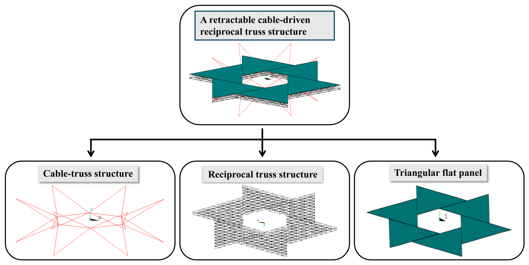
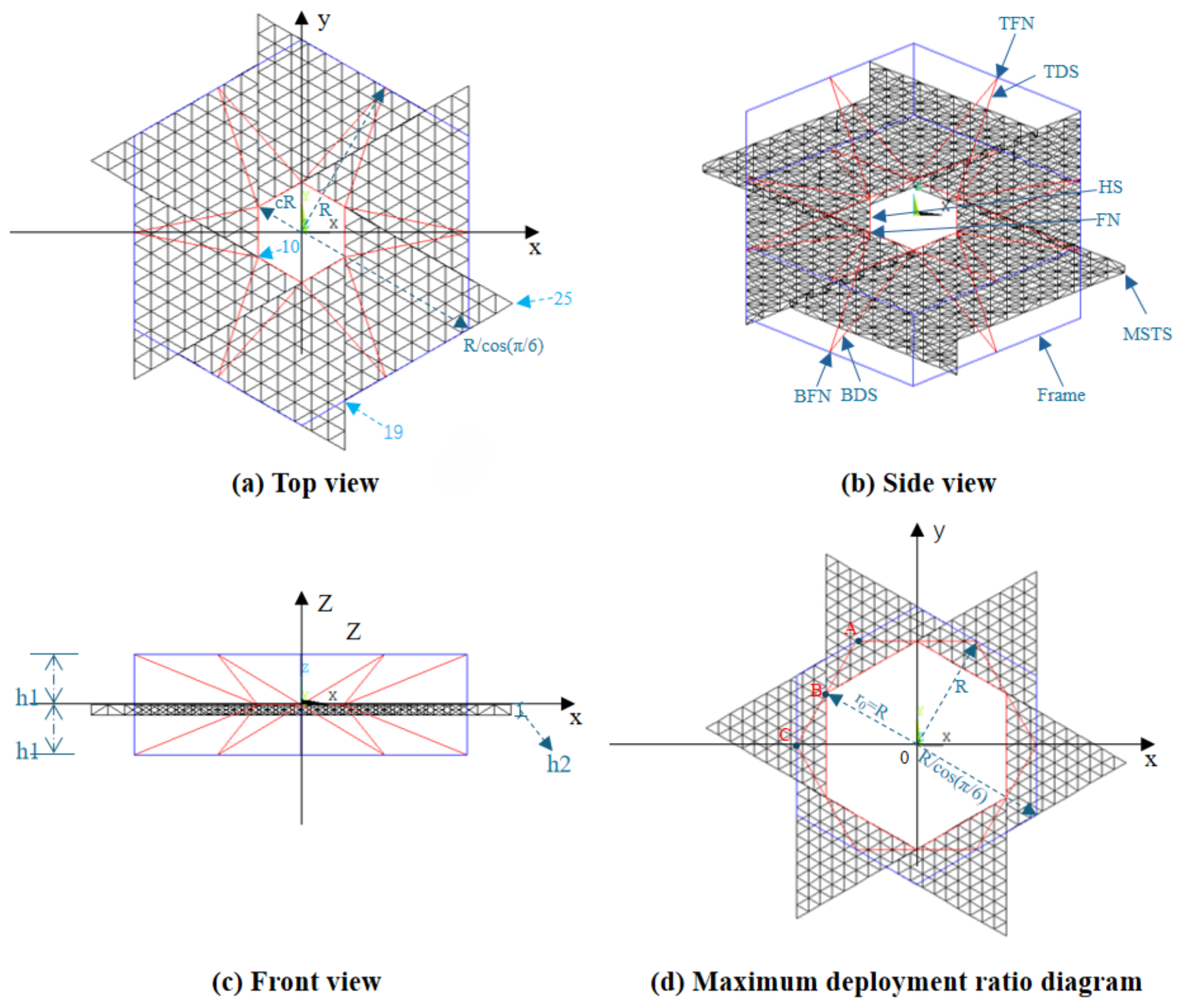
Figure 1 shows the proposed retractable cable-driven reciprocal truss, which consists of a cable-truss structure and a triangular reciprocal truss panel system. The panel structure is composed of a reciprocal truss and triangular planar panels that are rigidly connected to the top of the reciprocal truss. The cable-truss structure is formed by three continuous cables: a hoop cable, an upper diagonal cable, and a lower diagonal cable. These cables are connected at the inner ring nodes, and their bent segments are redirected by pulleys, thereby reducing the number of actuators and enabling the opening and closing motion of the structure. One upper corner node of the panel structure is connected to an inner ring node of the cable-truss structure, while the other two upper corner nodes are connected to the external frame. In terms of material properties, both the cable-truss structure and the reciprocal truss are made of steel ($E=2.06\times {10}^{11}\mathrm{Pa}$, $\nu =0.3$, $\rho =7870\mathrm{kg}/{\mathrm{m}}^3$). The cross-sectional area of the cables is $0.021715{\mathrm{m}}^2$, equivalent to three circular strands each with a diameter of $9.6\mathrm{cm}$. The beams have a hollow square cross-section of $0.1\mathrm{m}\times 0.1\mathrm{m}\times 0.01\mathrm{m}$, and the triangular planar panels have a thickness of $0.002\mathrm{m}$. This configuration reduces structural self-weight, utilizes the lightweight and high-strength properties of steel, and it provides a more realistic finite element model for engineering applications.

Based on the structural description above, the topological relationship of the established retractable cable-driven reciprocal truss structure is shown in Figure 2. In the top view shown in Figure 2a, the external fixed nodes of the cable-truss structure are located at the center of the horizontal frame, and the outer edge of the mutually supported truss structure (MSTS) is parallel to the external frame. The side view in Figure 2b shows that the cable-truss structure contains three types of nodes: top fixed nodes (TFN), bottom fixed nodes (BFN), and ring-shaped free nodes (FN). It also includes three types of cables: upper diagonal cables (TDS), bottom diagonal cables (BDS), and the hoop cable (HS). The numbers of these node types and cable types are consistent. The front view in Figure 2c shows that the inner ring nodes of the cable-truss structure and the upper nodes of the reciprocal truss are positioned at the center of the external frame.

Morphological design refers to the determination of the structural geometry under ideal conditions through structural topology, deployment trajectory, structural prestress, and cable-length adjustment, thereby defining the shape and topological relationships of the retractable cable-driven reciprocal truss structure.

To model the structure accurately, the center of the inner ring of the cable-truss structure is taken as the coordinate origin. The horizontal coordinates of the top fixed nodes (TFN) and bottom fixed nodes (BFN) of the cable-truss structure satisfy the following equation:

$$x^2+y^2=R^2$$

(1)

where R is the horizontal distance from the fixed node to the origin.

The free nodes are uniformly distributed along the inner hoop cable, and their coordinates satisfy the following equation:

$$x^2+y^2+z^2={\left(cR\right)}^2=r_0^2$$

(2)

where c is the deployment ratio, defined as the ratio of the radius of the circle along which the hoop cable is arranged to the radius of the circle along which the diagonal cables are arranged, as shown in Figure 2a. The range of c is $(0,c_{\max })$, where $c_{\max }$ denotes the maximum deployment ratio:

$$c_{\max }=\cos (\pi /6)$$

(3)

As shown in Figure 2d, when the inner ring node B is exactly aligned with the line connecting outer-ring nodes A and C in the top view, the cable-truss structure reaches its maximum deployment ratio. This geometric configuration represents the ultimate position of the structure under ideal conditions. If the deployment ratio increases further, the cable forces will become negative, indicating that the cables would begin to sustain compression, which contradicts the practical behavior of cables, as they are designed to sustain tension only.

For the cable-truss structure, the coordinates of the free node ${\mathit{n}}_a$, the top fixed node ${\mathit{n}}_{b1}$, and the bottom fixed node ${\mathit{n}}_{b2}$ at the i-th position can be obtained by solving Equations (4)–(6):

$$\begin{array}{cc}\hfill & {\mathit{n}}_{a,i}={\left[\begin{array}{ccc}\cos \alpha & -\sin \alpha & 0\\ \sin \alpha & \cos \alpha & 0\\ 0& 0& 1\end{array}\right]}^{i-1}\left[\begin{array}{ccc}\cos \beta & -\sin \beta & 0\\ \sin \beta & \cos \beta & 0\\ 0& 0& 1\end{array}\right]\left[\begin{array}{c}cR\\ 0\\ 0\end{array}\right]\hfill \end{array}$$

(4)

$$\begin{array}{cc}\hfill & {\mathit{n}}_{b1,i}={\left[\begin{array}{ccc}\cos \alpha & -\sin \alpha & 0\\ \sin \alpha & \cos \alpha & 0\\ 0& 0& 1\end{array}\right]}^i\left[\begin{array}{c}R\hfill \\ 0\hfill \\ h_1\hfill \end{array}\right]\hfill \end{array}$$

(5)

$$\begin{array}{cc}\hfill & {\mathit{n}}_{b2,i}={\left[\begin{array}{ccc}\cos \alpha & -\sin \alpha & 0\\ \sin \alpha & \cos \alpha & 0\\ 0& 0& 1\end{array}\right]}^i\left[\begin{array}{c}R\\ 0\\ -h_1\end{array}\right]\hfill \end{array}$$

(6)

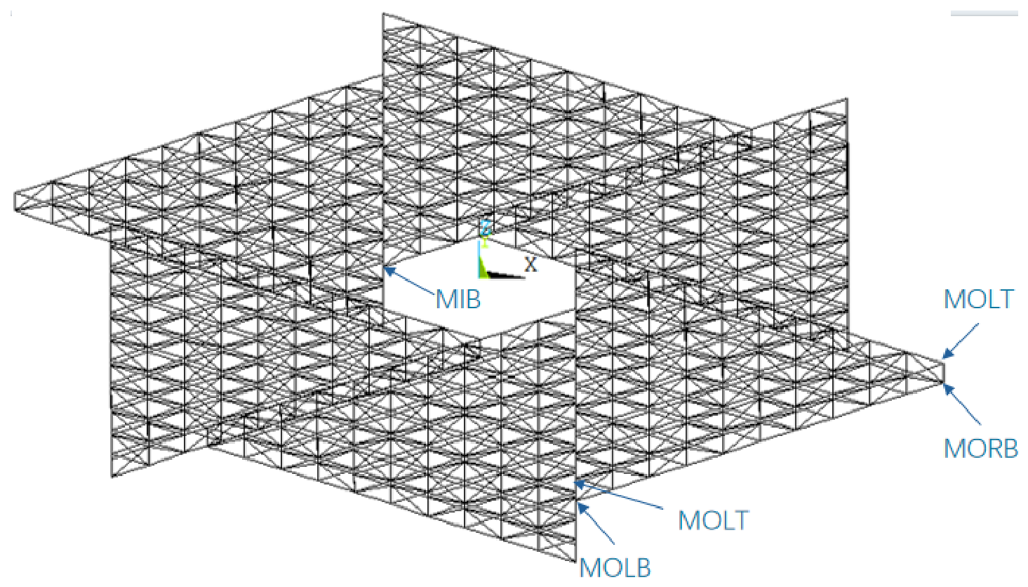
where $\alpha ={60}^{\circ }$ and $\beta ={30}^{\circ }$. As shown in Figure 3, the reciprocal truss structure consists of six triangular truss units. Each triangular truss unit is composed of six corner nodes: a free node (FN), a mutual inner bottom node (MIB), a mutual outer left top node (MOLT), a mutual outer left bottom node (MOLB), a mutual outer right top node (MORT), and a mutual outer right bottom node (MORB).

For the i-th triangular truss unit of the reciprocal truss structure, the coordinates of the mutual inner bottom node ${\mathit{n}}_{MIB}$, the mutual outer left top node ${\mathit{n}}_{MOLT}$, the mutual outer left bottom node ${\mathit{n}}_{MOLB}$, the mutual outer right top node ${\mathit{n}}_{MORT}$, and the mutual outer right bottom node ${\mathit{n}}_{MORB}$ can be obtained using the following equations:

$$\begin{array}{cc}\hfill & {\mathit{n}}_{MIB,i}={\left[\begin{array}{ccc}\cos \alpha & -\sin \alpha & 0\\ \sin \alpha & \cos \alpha & 0\\ 0& 0& 1\end{array}\right]}^{i-1}\left[\begin{array}{ccc}\cos \beta & -\sin \beta & 0\\ \sin \beta & \cos \beta & 0\\ 0& 0& 1\end{array}\right]\left[\begin{array}{c}cR\\ 0\\ h_2\end{array}\right]\hfill \end{array}$$

(7)

$$\begin{array}{cc}\hfill & {\mathit{n}}_{MOLT,i}={\left[\begin{array}{ccc}\cos \alpha & -\sin \alpha & 0\\ \sin \alpha & \cos \alpha & 0\\ 0& 0& 1\end{array}\right]}^{i-2}\left[\begin{array}{c}R\\ \mathrm{san}\sqrt{{\left({\displaystyle \frac{R}{\cos (\pi /6)}}-r_0\cos (\pi /3)\right)}^2+r_0^2{\sin }^2(\pi /3)-R^2}\\ 0\end{array}\right]\hfill \end{array}$$

(8)

$$\begin{array}{cc}\hfill & {\mathit{n}}_{MOLB,i}={\left[\begin{array}{ccc}\cos \alpha & -\sin \alpha & 0\\ \sin \alpha & \cos \alpha & 0\\ 0& 0& 1\end{array}\right]}^{i-2}\left[\begin{array}{c}R\\ \mathrm{san}\sqrt{{\left({\displaystyle \frac{R}{\cos (\pi /6)}}-r_0\cos (\pi /3)\right)}^2+r_0^2{\sin }^2(\pi /3)-R^2}\\ h_2\end{array}\right]\hfill \end{array}$$

(9)

$$\begin{array}{cc}\hfill & {\mathit{n}}_{MORT,i}=\left[\begin{array}{ccc}\cos \alpha & -\sin \alpha & 0\\ \sin \alpha & \cos \alpha & 0\\ 0& 0& 1\end{array}\right]\left[\sqrt{{\displaystyle \frac{R}{{\left(\frac{R}{\cos (\pi /6)}+r_0\cos (\pi /3)\right)}^2+r_0^2{\sin }^2(\pi /3)-R^2}}}\right]\hfill \end{array}$$

(10)

$$\begin{array}{cc}\hfill & {\mathit{n}}_{MORB,i}={\left[\begin{array}{ccc}\cos \alpha & -\sin \alpha & 0\\ \sin \alpha & \cos \alpha & 0\\ 0& 0& 1\end{array}\right]}^{i-2}\left[\begin{array}{c}R\\ \sqrt{{\left({\displaystyle \frac{R}{\cos (\pi /6)}}+r_0\cos (\pi /3)\right)}^2+r_0^2{\sin }^2(\pi /3)-R^2}\\ h_2\end{array}\right]\hfill \end{array}$$

(11)

where $\mathrm{san}=1$ when the deployment ratio $c⩾\tan {30}^{\circ }$, and $\mathrm{san}=-1$ otherwise.

In the theoretical analysis, a structure with a node-level height of $h_1=15\mathrm{m}$, a reciprocal truss height of $h_2=3\mathrm{m}$, and a radius of $R=50\mathrm{m}$ is considered.

2.2. Structural Topology

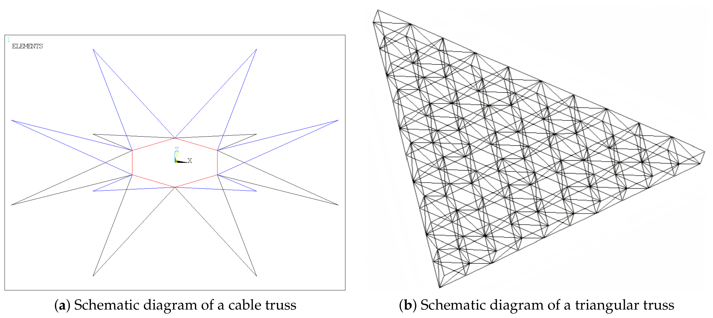
As shown in Figure 2b, the retractable cable-driven reciprocal truss consists of a cable-truss structure and a reciprocal truss. The cable-truss structure drives the opening and closing motion of the overall structure (Figure 4a). In the figure, the upper diagonal cables are shown in blue, the bottom diagonal cables in black, and the hoop cables in red. Each upper diagonal cable (TDS) element connects an adjacent upper fixed node ${\mathit{n}}_{b1}$ to a free node ${\mathit{n}}_a$; each bottom diagonal cable (BDS) element connects an adjacent lower fixed node ${\mathit{n}}_{b2}$ to the free node ${\mathit{n}}_a$; and each hoop cable (HS) element connects two adjacent free nodes ${\mathit{n}}_a$. Diagonal cables of the same type are continuous, i.e., a single full-length cable replaces them, and the three full-length cables are connected at the free nodes. The bent segments of each cable are redirected by pulleys, thereby reducing the number of actuators and enabling the opening and closing motion of the structure.

Each triangular truss unit of the reciprocal truss consists of two planar triangular trusses (Figure 4b), which are assembled from small equilateral triangular trusses as basic units. The side length of each equilateral triangular truss is one-tenth ($5\mathrm{m}$) of the planar side length of the triangular truss, and the beams of the truss structure are rigidly connected. The corresponding nodes of the equilateral triangular trusses in the two planar triangular truss layers are connected by vertical members, each with a length of $h_2$, and adjacent vertical members are connected by diagonal members with a length of $\sqrt{5^2+h_2^2}$. As shown in Figure 2b, Node 19 is the endpoint of the upper planar triangular truss. The triangular trusses are connected via sliders located at Node 19, so that Node 19 always lies on the straight line connecting the free node to the upper-right outer-ring node of the reciprocal truss structure. Moreover, the nodes on the beam element connecting the upper-left outer-ring node and the upper-right outer-ring node of the reciprocal truss structure are connected to the external frame via slider units, allowing these nodes to move only along the straight line defined by the two outer-ring nodes.

The reciprocal truss and the cable-truss structure are connected at the free nodes ${\mathit{n}}_a$. By adjusting the cable lengths of the cable-truss structure, the free nodes drive the opening and closing motion of the reciprocal truss structure, thereby realizing the retractable motion of the cable-driven reciprocal truss structure.

2.3. Deployment Trajectory

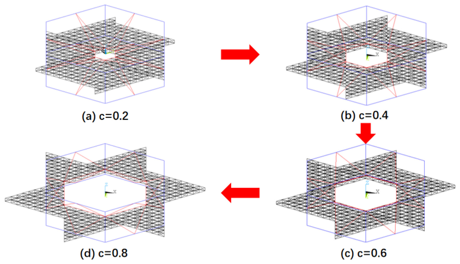
For smooth opening and closing, the inner-ring free nodes (FN) of the cable-truss structure must remain in the horizontal plane passing through the origin, and the structure must maintain rotational symmetry throughout the process. As shown in the structural opening and closing diagram in Figure 5, as the deployment ratio increases, the structure opens; the lengths of the upper and lower diagonal cables of the cable-truss structure decrease continuously and equally, while the length of the hoop cable increases continuously. Simultaneously, the reciprocal truss structure moves outward along the frame, while its beam dimensions remain unchanged. Conversely, as the deployment ratio decreases, the lengths of the upper and lower diagonal cables of the cable-truss structure increase continuously and equally, while the length of the hoop cable decreases continuously. At the same time, the reciprocal truss structure moves inward along the frame, while its beam dimensions remain unchanged.

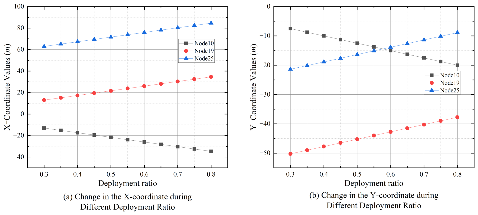
To study the kinematic behavior quantitatively under ideal conditions, three key nodes, namely, Node 10, Node 19, and Node 25 in Figure 2a, are selected for coordinate analysis. These three key nodes are located in different stress-bearing regions, allowing the structural motion trajectories under different values of the deployment ratio to be better represented and the relationship between the nodal coordinates and the deployment ratio to be established, as shown in Figure 6. Node 10 lies in the third quadrant, whereas Nodes 19 and 25 lie in the fourth quadrant. The X- and Y-coordinates of all three nodes vary linearly with the deployment ratio. The coordinates of Nodes 19 and 25 increase linearly, while those of Node 10 show the opposite trend. Throughout the motion, the Z-coordinate of each node remains zero for any value of the deployment ratio, indicating that the ring nodes of both the reciprocal truss and the cable-truss structure move only in a plane. Hence, under ideal conditions, where external loads and self-weight are ignored, the ring nodes of both structures move along straight lines in their common plane, and the displacement varies linearly with the deployment ratio. Therefore, the motion is simple and highly regular.

By substituting $i=4$, $i=1$, and $i=1$ into Equations (4), (8) and (10), respectively, the coordinate formulas for Node 10, Node 19, and Node 25 are obtained as follows:

$$\begin{array}{cc}\hfill & \left[\begin{array}{c}{x}_{10}\hfill \\ y_{10}\hfill \\ z_{10}\hfill \end{array}\right]={\left[\begin{array}{ccc}\cos \alpha & -\sin \alpha & 0\\ \sin \alpha & \cos \alpha & 0\\ 0& 0& 1\end{array}\right]}^3\left[\begin{array}{ccc}\cos (\pi /6)& -\sin (\pi /6)& 0\\ \sin (\pi /6)& \cos (\pi /6)& 0\\ 0& 0& 1\end{array}\right]\left[\begin{array}{c}cR\\ 0\\ 0\end{array}\right]\hfill \end{array}$$

(12)

$$\begin{array}{cc}\hfill & \left[\begin{array}{c}{x}_{19}\hfill \\ y_{19}\hfill \\ z_{19}\hfill \end{array}\right]={\left[\begin{array}{ccc}\cos \alpha & -\sin \alpha & 0\\ \sin \alpha & \cos \alpha & 0\\ 0& 0& 1\end{array}\right]}^{-1}\left[\begin{array}{c}R\\ \mathrm{san}\sqrt{{\left({\displaystyle \frac{R}{\cos (\pi /6)}}-cR\cos (\pi /3)\right)}^2+{\left(cR\right)}^2{\sin }^2(\pi /3)-R^2}\\ 0\end{array}\right]\hfill \end{array}$$

(13)

$$\begin{array}{cc}\hfill & \left[\begin{array}{c}{x}_{25}\hfill \\ y_{25}\hfill \\ z_{25}\hfill \end{array}\right]={\left[\begin{array}{ccc}\cos \alpha & -\sin \alpha & 0\\ \sin \alpha & \cos \alpha & 0\\ 0& 0& 1\end{array}\right]}^{-1}\left[\begin{array}{c}R\\ \sqrt{{\left({\displaystyle \frac{R}{\cos (\pi /6)}}+cR\cos (\pi /3)\right)}^2+{\left(cR\right)}^2{\sin }^2(\pi /3)-R^2}\\ 0\end{array}\right]\hfill \end{array}$$

(14)

2.4. Structural Prestress

Although the previous subsection defined the kinematic path, the structural prestress ${\overline{\mathit{t}}}_a$ must also be designed to ensure proper opening and closing. A prescribed prestress is applied to each cable in the cable-truss structure. For the hoop cable, the prestress must satisfy the following [45]:

$${\mathit{E}}_a^{\mathrm{T}}{\mathit{A}}_{2c}{\mathit{t}}_c={\mathit{w}}_a$$

(15)

where the equilibrium matrix ${\mathit{A}}_{2c}\in {\mathit{R}}^{3n_n\times n_{ec}}$ is detailed in [45].

Here, ${\mathit{w}}_a=\left({\mathit{f}}_{ex}-\mathit{g}\right)$ is the total external load at the free nodes. ${\mathit{f}}_{ex}$ denotes the external load vector at the nodes, and $\mathit{g}$ is the gravity vector corresponding to the free nodes. Performing singular value decomposition on the equilibrium matrix ${\mathit{E}}_a^{\mathrm{T}}{\mathit{A}}_{2c}\in {\mathit{R}}^{n_a\times n_{ec}}$ for the free nodes yields the following [45]:

$${\mathit{E}}_a^{\mathrm{T}}{\mathit{A}}_{2c}=\mathit{U}\mathbf{\Sigma }{\mathit{V}}^{\mathrm{T}}=\left[{\mathit{U}}_1,{\mathit{U}}_2\right]\left[\begin{array}{cc}{\mathbf{\Sigma }}_0& 0\\ 0& 0\end{array}\right]\left[\begin{array}{c}{\mathit{V}}_1^{\mathrm{T}}\hfill \\ {\mathit{V}}_2^{\mathrm{T}}\hfill \end{array}\right]$$

(16)

where $\mathit{U}\in {\mathit{R}}^{n_a\times n_a}$ and $\mathit{V}\in {\mathit{R}}^{n_{ec}\times n_{ec}}$ are orthogonal matrices. The matrices ${\mathit{V}}_1\in {\mathit{R}}^{n_{ec}\times r}$, ${\mathit{V}}_2\in {\mathit{R}}^{n_{ec}\times \left(n_{ec}-r\right)}$, ${\mathit{U}}_1\in {\mathit{R}}^{n_a\times r}$, ${\mathit{U}}_2\in {\mathit{R}}^{n_a\times \left(n_a-r\right)}$, and ${\mathbf{\Sigma }}_0\in {\mathit{R}}^{r\times r}$ represent the row space, null space, column space, left null space, and singular values of the equilibrium matrix, respectively. These matrices are obtained from the decomposition of the orthogonal matrices $\mathit{U}$ and $\mathit{V}$ and the rectangular matrix $\mathbf{\Sigma }$, which is composed of diagonal and zero blocks. Here, r is the rank of the equilibrium matrix ${\mathit{E}}_a^{\mathrm{T}}{\mathit{A}}_{2c}$. The solution to the equilibrium equation is given in the following [45]:

$${\mathit{t}}_c={\left({\mathit{E}}_a^{\mathrm{T}}{\mathit{A}}_{2c}\right)}^{+}{\mathit{w}}_a+{\mathit{V}}_2\mathit{z}$$

(17)

where the superscript ${\ast }^{+}$ denotes the pseudoinverse of a matrix ∗. The term ${\mathit{t}}_{c1}={\left({\mathit{E}}_a^{\mathrm{T}}{\mathit{A}}_{2c}\right)}^{+}{\mathit{w}}_a$ is the particular solution obtained from the external loads, and ${\mathit{t}}_{c2}={\mathit{V}}_2\mathit{z}$ is the complementary solution derived from the prestress. Furthermore, solving the null space of the equilibrium matrix ${\mathit{V}}_2$ yields the self-stress coefficients $\mathit{z}\in {\mathit{R}}^{n_{ec}-r}$. If the prestress of $n_{ec}-r$ members is specified as ${\mathit{t}}_d$, and the matrix ${\mathit{e}}_d$ is used to extract the prestress of specific members of the cable-truss structure, then [45],

$${\mathit{t}}_d={\mathit{e}}_d^{\mathrm{T}}{\mathit{t}}_c$$

(18)

Substituting Equation (14) into Equation (15) yields the following [45]:

$${\overline{\mathit{t}}}_d={\mathit{e}}_d^{\mathrm{T}}{\left({\mathit{E}}_a^{\mathrm{T}}{\mathit{A}}_{2c}\right)}^{+}{\mathit{w}}_a+{\mathit{e}}_d^{\mathrm{T}}{\mathit{V}}_2\mathit{z}$$

(19)

Then the self-stress coefficient $\mathit{z}$ is as follows [45]:

$$\mathit{z}=\left({\mathit{e}}_d^{\mathrm{T}}{\mathit{V}}_2\right)\left[{\overline{\mathit{t}}}_d-{\mathit{e}}_d^{\mathrm{T}}{\left({\mathit{E}}_a^{\mathrm{T}}{\mathit{A}}_{2c}\right)}^{+}{\mathit{w}}_a\right]$$

(20)

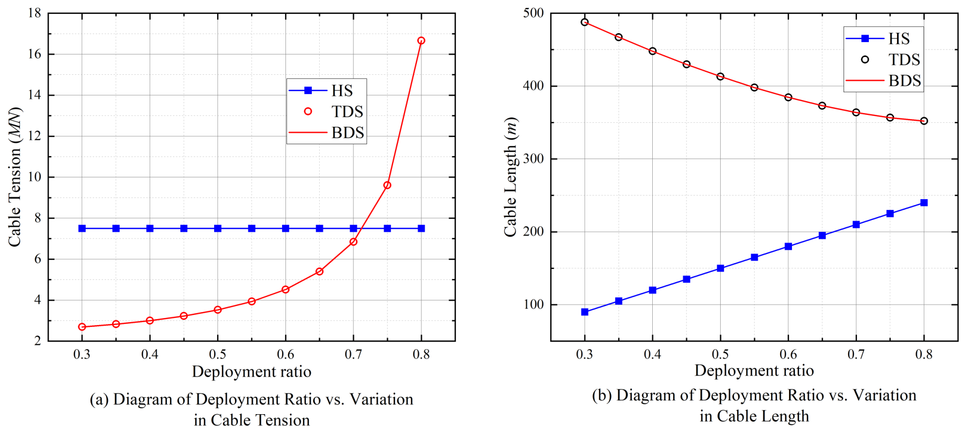
Substituting Equation (20) into Equation (17) yields the member force vector $\mathit{t}$ of the structure. For a cable-truss structure, all cable members must remain in tension; that is, their axial internal forces must be positive. To accurately realize the opening and closing motion of the structure and simplify the cable-length adjustment strategy, the prestress of the hoop cable is maintained at a constant value of ${\overline{\mathit{t}}}_d=7.5\mathrm{MN}$. 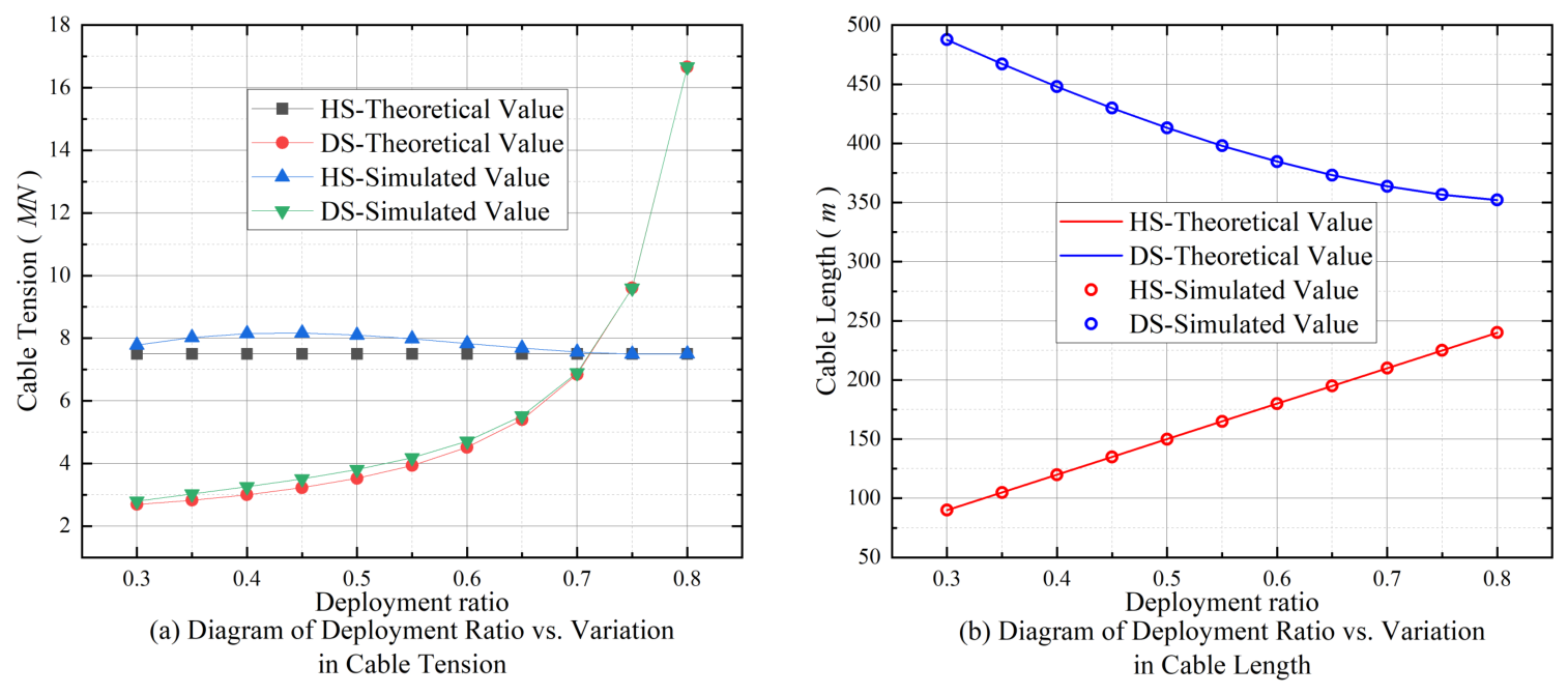Consequently, the relationships between the deployment ratio and the cable force (Figure 7a) and between the deployment ratio and the cable length (Figure 7b) are obtained. As shown in the figures, the prestress of the diagonal cables exhibits a nonlinear increasing trend as the deployment ratio increases, and the slope gradually increases. This indicates that when the structure approaches its maximum deployment ratio, the internal force in the diagonal cables increases sharply and tends to infinity as the deployment ratio approaches the maximum.

The cable force must remain positive and below the tensile capacity (tensile strength × cross-sectional area). The steel cable has a tensile strength of $1670\mathrm{MPa}$, giving a maximum sustainable force of $36.263\mathrm{MN}$. In this study, the maximum cable force is below $19\mathrm{MN}$, indicating a sufficient safety margin. Therefore, to ensure structural stability and proper opening and closing, the deployment ratio is limited to the range of $0.3$–$0.8$. The length of the hoop cable increases linearly with the deployment ratio, while the length of the diagonal cable decreases nonlinearly. This is because the hoop cable involves only the ring nodes, which vary linearly with the deployment ratio, whereas the diagonal cable involves both ring nodes and fixed nodes, with its length determined by the Euclidean distance formula. Hence, as the deployment ratio increases, the rate of decrease in the diagonal cable length gradually diminishes, i.e., the absolute slope of the curve decreases. The prestress and length of the upper and lower diagonal cables remain equal throughout, further verifying the geometric symmetry of the structure under ideal conditions.

2.5. Cable-Length Adjustment Strategy

To enable proper opening and closing along the trajectory shown in Figure 5, a simple cable-length adjustment method is established based on the following assumptions:

(1)

There is no friction between the cables and the pulleys, and no friction between the sliders and the reciprocal trusses.

(2)

In the theoretical model, the dimensions of the pulleys, sliders, and the connecting components between the pulleys are negligible.

It should also be noted that friction can lead to uneven transmission of cable forces, causing deviations between the theoretically calculated relationship between cable length and driving force and the actual values required during operation. This may affect the accuracy of the opening and closing trajectory. Actual components have certain geometric dimensions; in particular, the radii of pulleys and the thickness of sliders can alter the actual moment arm and kinematic geometry of the cables. This introduces nonlinear errors in the theoretical linear relationship between cable length variation and nodal displacement and may further cause kinematic interference or local stress concentration due to changes in the spatial configuration of the connectors during the opening and closing process of the structure.

Under these assumptions, during any opening and closing process, the unstressed length ${\mathit{l}}_{0c}$ of the cable can be obtained from the cable force ${\mathit{t}}_c$ and the cable length ${\mathit{l}}_c$ of the full-length cable in the cable-truss structure [45]:

$${\mathit{l}}_{0c}={\left({\widehat{\mathit{t}}}_c+{\widehat{\mathit{E}}}_c{\widehat{\mathit{A}}}_c\right)}^{-1}{\widehat{\mathit{E}}}_c{\widehat{\mathit{A}}}_c{\widehat{\mathit{l}}}_c$$

(21)

where ${\mathit{A}}_c$ is the cross-sectional area vector of the cable-truss structure, and ${\mathit{E}}_c$ is its Young’s modulus vector.

Based on the analysis of the theoretical model described above, the relationship between the deployment ratio c and the length of the full-length cables can be established. As shown in Figure 7b, as the deployment ratio increases, the length of the hoop cable increases continuously, while the length of the diagonal cables decreases continuously. This opposite variation in the lengths of the hoop and diagonal cables with changes in the deployment ratio reflects the cable-length adjustment strategy of the structure. To maintain a constant internal force in the hoop cable, the hoop cable elongates or contracts as the deployment ratio increases or decreases, respectively. In contrast, the diagonal cables undergo corresponding contraction or elongation according to the geometric relationship.

3. Mechanical Performance Analysis of the Structure

In this chapter, the natural vibration modes of the structure are analyzed. Taking the structure with a deployment ratio of $c=0.5$ as an example, the natural frequencies and the corresponding mode shape characteristics are examined. In the following subsection, parametric analyses are performed on selected structural parameters, including the deployment ratio, external load, prestress, beam Section depth, truss height, and cable cross-sectional area. Meanwhile, the self-weight of the structure, the live load on the non-accessible roof, and the panel load are incorporated into the simulation to improve the realism of the numerical model. The maximum displacement and cable force distribution of the structure under varying parameters are obtained to evaluate the influence of each parameter and identify appropriate measures when the structural response does not meet the design requirements. To ensure comparability among the figures, the deployment ratio is limited to the range $0.3\le c\le 0.8$ in the corresponding plots, and data are extracted at deployment-ratio intervals of 0.05.

3.1. Natural Vibration Modal Analysis

For structures containing prestressed cables, the stress-stiffening effect must be considered in the modal analysis. Therefore, prestressed modal analysis is carried out in ANSYS APDL using the following procedure. First, static analysis is performed with the prestress effect enabled. The solver is then re-entered, and the PSTRES, ON command is used to enable the prestress effect and obtain the modal analysis solution. Finally, the natural frequencies and mode shapes are obtained through the general postprocessor. The natural vibration modes and frequencies of the structure are obtained from the generalized eigenvalue analysis [45]:

$${\mathit{K}}_{T_{aa}}{\mathsf{\phi }}_j={\omega }_j^2{\mathit{M}}_{aa}{\mathsf{\phi }}_j$$

(22)

where ${\omega }_j$ is the natural frequency of the j-th structural mode, and ${\mathsf{\phi }}_j$ is the corresponding mode shape vector. The mass matrix for the free nodes is given by ${\mathit{M}}_{aa}={\mathit{E}}_a^{\mathrm{T}}\mathit{M}{\mathit{E}}_a$, where the mass matrix $\mathit{M}\in {\mathit{R}}^{3n_n\times 3n_n}$ of the cable-truss structure is given in [45].

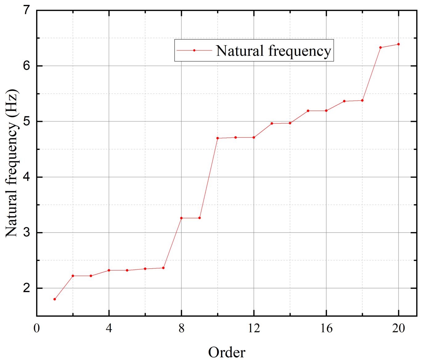
For a hoop cable force of $7.5\mathrm{MN}$ and a deployment ratio of $c=0.5$, the natural frequencies are listed in Figure 8 and

Table 1. Structural natural frequencies.

Order	Natural Frequency (Hz)	Order	Natural Frequency (Hz)
1	1.8012627	11	4.7102742
2	2.2216058	12	4.7105781
3	2.2226403	13	4.9646588
4	2.3200958	14	4.9685219
5	2.321137	15	5.1917953
6	2.3486546	16	5.1950435
7	2.3647814	17	5.3641262
8	3.2623566	18	5.3780755
9	3.2630964	19	6.3291172
10	4.6993609	20	6.3903949

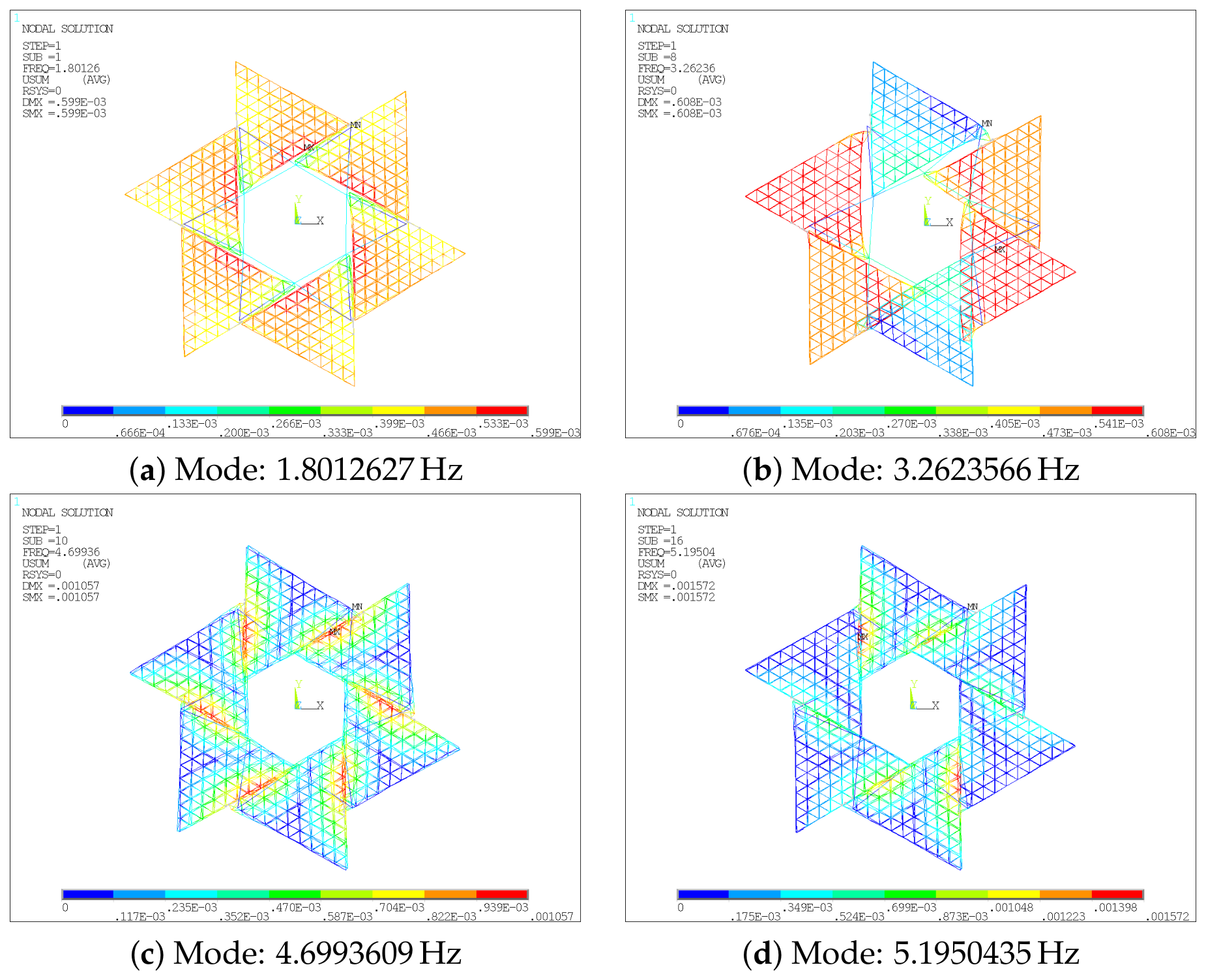
, while the corresponding mode shapes are shown in Figure 9. Specifically, Figure 9 presents the natural frequencies and mode shapes of the 1st, 8th, 10th, and 16th modes. For the 1st mode, the natural frequency is $1.8012627\mathrm{Hz}$ (Figure 9a), and the structure undergoes global symmetric deformation characterized by overall structural expansion. Although downward displacement occurs at the red locations, the overall structure expands outward. For the 8th mode, the natural frequency is $3.2623566\mathrm{Hz}$ (Figure 9b). The structure exhibits local symmetric deformation, with different deformation patterns in adjacent triangular trusses, and the truss with the maximum displacement moves leftward. For the 10th mode, the natural frequency is $4.6993609\mathrm{Hz}$ (Figure 9c). The structure exhibits centrosymmetric deformation, and the maximum displacement is located at the contact points of the trusses, with the displacement direction mainly along the Z-axis. For the 16th mode, the natural frequency is $5.1950435\mathrm{Hz}$ (Figure 9d). The structure undergoes local centrosymmetric deformation; that is, the deformations of triangular trusses symmetric with respect to the origin are centrally symmetric. When one truss displaces downward, the corresponding symmetric truss displaces upward.

3.2. Mechanical Analysis Under External Load

In the mechanical analysis, the magnitude of the external load is a key factor affecting the structural response.

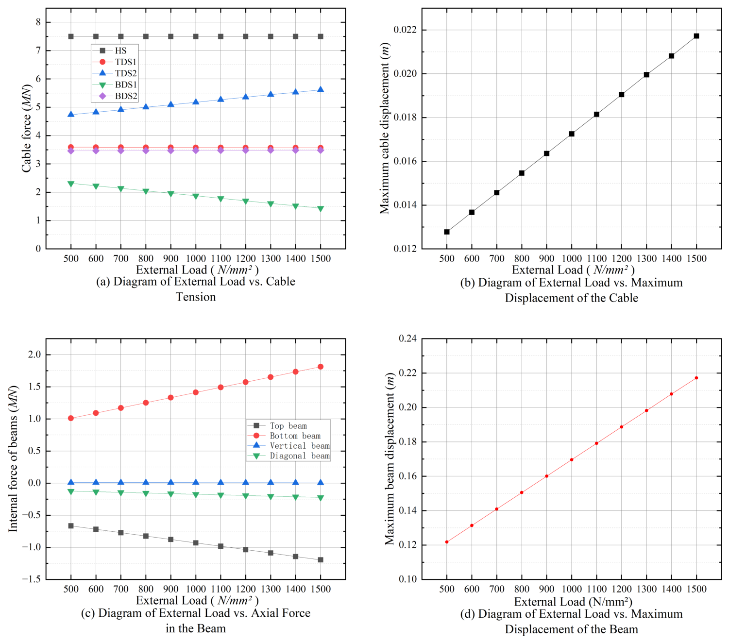
As shown in Figure 10d, the maximum displacement of the structure increases linearly with the external load. This trend can be explained by the relationship $\delta \propto {\delta }_1+{\delta }_2$ from the truss deflection analysis, where ${\delta }_1\propto {\displaystyle \frac{q{L}^4}{E{I}_{eq}}}$ and ${\delta }_2\propto {\displaystyle \frac{FL}{EA}}$. First, the surface load acting on the triangular planar panel is defined as $q^{\prime }$. It is then converted into an equivalent line load acting on the reciprocal truss beam, given by $q={\displaystyle \frac{\sqrt{3}{q}^{\prime }L}{12}}$. The force acting on the diagonal cable satisfies $F\propto q^{\prime }{L}^2$. In this parametric analysis, all other quantities in the formulas remain constant, while only the surface load $q^{\prime }$ acting on the triangular planar panel increases linearly. Therefore, both the equivalent line load and the force acting on the diagonal cable increase linearly with the surface load, leading to a linear increase in the maximum displacement of the structure.

As shown in Figure 10b, as the external load increases linearly, the equivalent vertical load acting on the ring free nodes also increases linearly, resulting in a linear increase in the maximum displacement of the cable-truss structure, i.e., the displacement of the ring nodes.

As shown in Figure 10a, the internal force in the hoop cable remains nearly unchanged. Unlike the hoop cable, whose response is mainly associated with lateral load transfer and displacement, the diagonal cables respond to both vertical and lateral loads as well as the associated deformation. Therefore, the magnitude of the external load has a significant influence on them. As the external load increases linearly, the internal forces in the individual diagonal cables also change linearly. Specifically, the internal forces in the upper diagonal cables increase linearly with the external load, while those in the lower diagonal cables decrease linearly. This reflects the characteristic internal force redistribution in the cable-truss structure under vertical load: when a vertical external load is applied, the upper diagonal cables are further tensioned and provide greater axial reaction forces, whereas the tension in the lower diagonal cables decreases, resulting in lower internal forces. Although the cable-truss structure is geometrically axisymmetric, the interaction with the reciprocal truss under vertical loading results in different internal forces in diagonal cables of the same type.

As shown in Figure 10c, as the external load increases linearly, the bending moment acting on the reciprocal truss structure also increases linearly. This leads to a linear increase in the absolute values of the axial forces in the top and bottom chords, consistent with the formula $N\propto M/h$. The axial forces in the diagonal and vertical members are also influenced by the vertical external load. As the external load increases, the axial compression in the diagonal members increases, whereas the internal force in the vertical members remains nearly unchanged.

When a uniformly distributed external vertical load is applied to the triangular planar panels, the original force equilibrium state is disrupted, and internal forces are redistributed to resist the external load while maintaining nodal equilibrium and deformation compatibility. The hoop cable is insensitive to vertical loads, and its axial force remains almost unchanged. The diagonal cables carry both vertical and lateral loads: the upper diagonal cables (TDS) exhibit a linear increase in axial force and provide vertical reaction forces, while the bottom diagonal cables (BDS) show a linear decrease in axial force, indicating partial unloading. Although the structure is axially symmetric, the responses of diagonal cables at different positions differ; specifically, the slopes of TDS2 and BDS1 are relatively large, whereas those of TDS1 and BDS2 are close to zero. The external load induces additional bending moments in the reciprocal truss, increasing the compressive axial forces in the top chords and diagonal members (more negative axial forces) and the tensile axial forces in the bottom chords (more positive axial forces). The absolute values of the axial forces in the top and bottom chords increase linearly with the external load ($N\propto M/h$), and the axial compressive forces in the diagonal members also increase linearly, reflecting the typical bending moment–axial force redistribution mechanism in truss structures. Through this redistribution, the structure effectively transfers shear forces and bending moments to the cables and truss members, which are ultimately transmitted to the fixed nodes and the outer frame via the cables. The entire redistribution process satisfies nodal equilibrium and deformation compatibility, with no local yielding or instability observed, indicating that the structure has sufficient internal force redistribution capacity and safety redundancy.

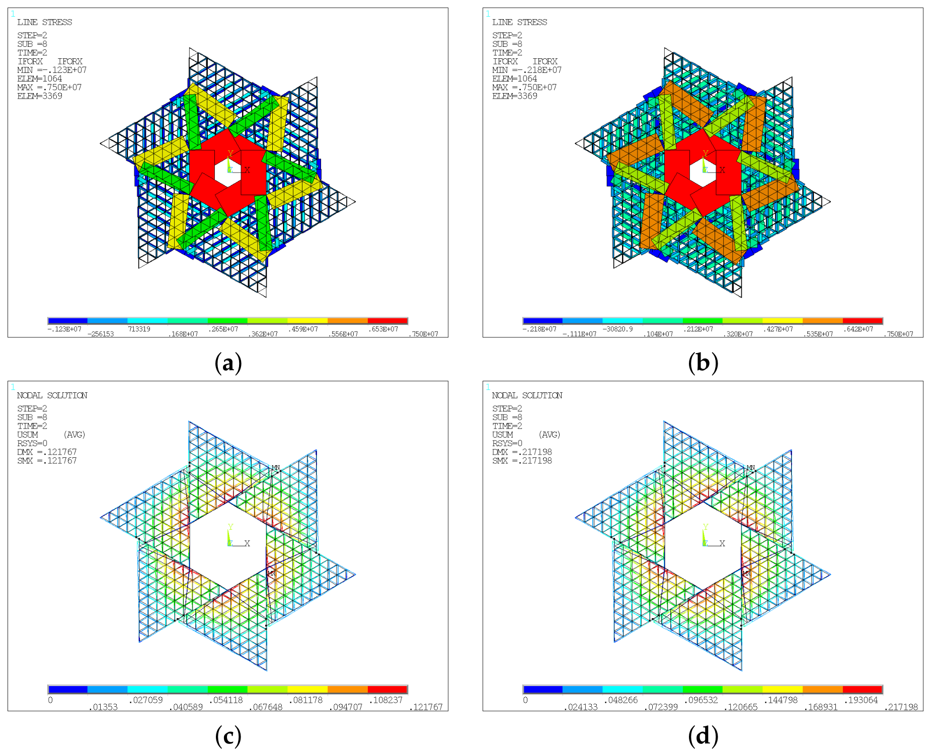
As shown in Figure 11, as the external load increases, the absolute values of the axial forces in the reciprocal truss and diagonal cables increase significantly, while the axial force in the hoop cable remains almost unchanged. Meanwhile, the distribution pattern of the structural deformation contour remains similar, but the numerical values corresponding to the colors increase by approximately $0.8$ times their original values. This indicates that, as the external load increases, the structural deformation becomes substantially larger, whereas its distribution pattern remains essentially unchanged.

In addition, it should be noted that when the external load reaches $1500\mathrm{N}/{\mathrm{m}}^2$, the maximum displacement of the structure is $0.217198\mathrm{m}$, which slightly exceeds the allowable design value of $0.2\mathrm{m}$ specified in the code Technical specification for space frame structures. Considering that the maximum displacement increases as the deployment ratio decreases, it is recommended that the external load applied to the reciprocal truss structure not exceed $900\mathrm{N}/{\mathrm{m}}^2$ to ensure the serviceability and safety of the structure during operation.

3.3. Parametric Analysis

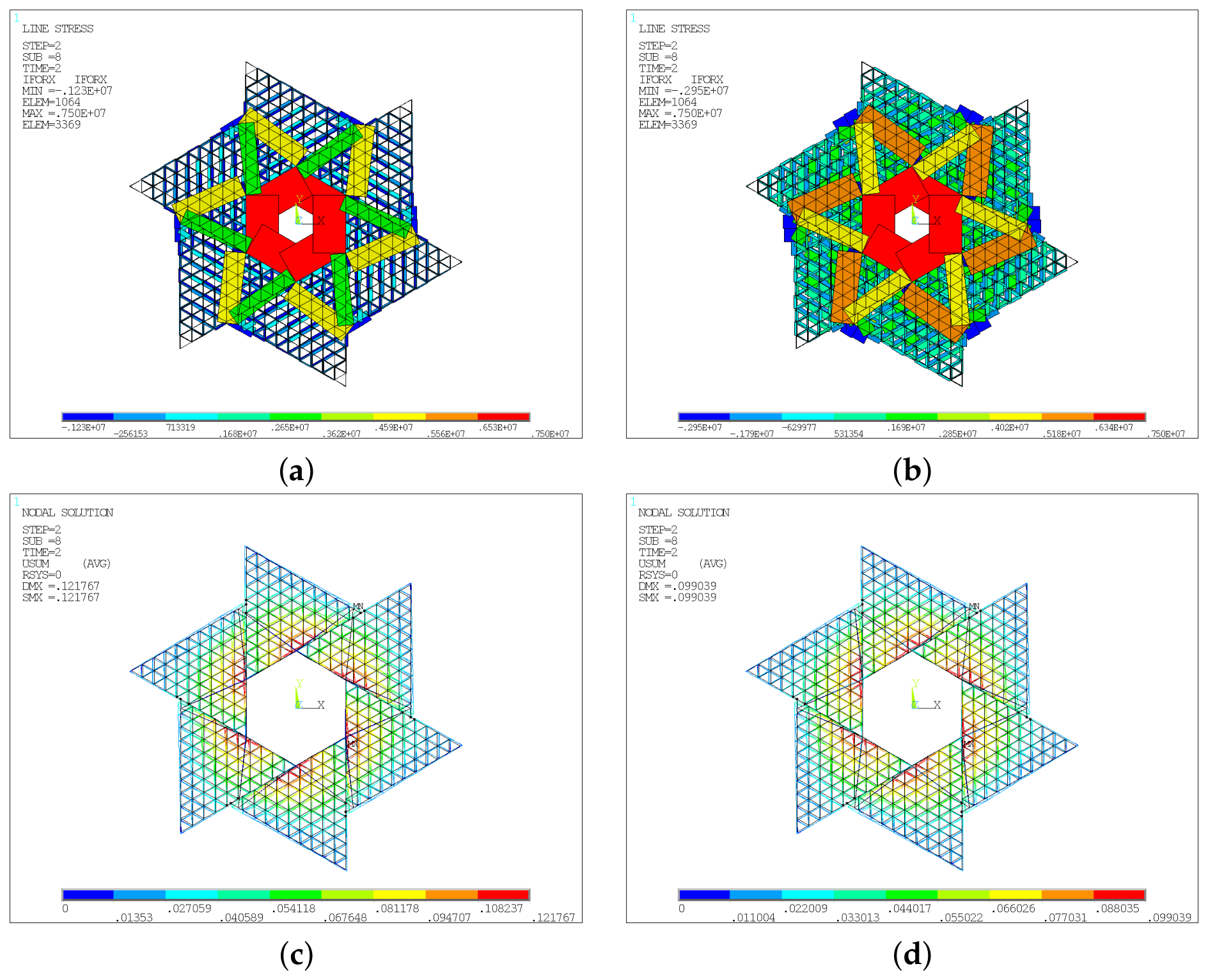
To analyze the influence of various parameters on the mechanical and deformation responses of the structure, this subsection examines six key parameters: deployment ratio, external load, prestress, truss height, cable cross-sectional area, and beam section depth. By varying one parameter at a time, the effect of each parameter on the structural response is evaluated, thereby providing theoretical guidance for the optimization of structural geometry and prestress design. To ensure comparability among the parametric analyses, a unified benchmark case is first defined for all parameter studies. This benchmark case is characterized by a deployment ratio of $c=0.5$, hoop cable prestress of $7.5\mathrm{MN}$, diagonal cable prestress of $3,526,692.354\mathrm{N}$, truss height of $3\mathrm{m}$ (with the Z-coordinate of the lower truss nodes at $-3\mathrm{m}$), and cable cross-sectional area of $0.021714688{\mathrm{m}}^2$ (three steel cables with a radius of $4.8\mathrm{cm}$ each). The beam cross-section is $0.1\mathrm{m}\times 0.1\mathrm{m}\times 0.01\mathrm{m}$, corresponding to a hollow square steel tube with a side length of $0.1\mathrm{m}$ and a wall thickness of $0.01\mathrm{m}$. The external load is $500\mathrm{N}/{\mathrm{m}}^2$. During the parametric analysis, only the corresponding parameter is varied, while all other parameters remain unchanged. For example, in the prestress analysis, only the prestress values are changed, while all other parameters remain as specified above.

3.3.1. Parametric Analysis of the Influence of the Deployment Ratio on Structural Performance

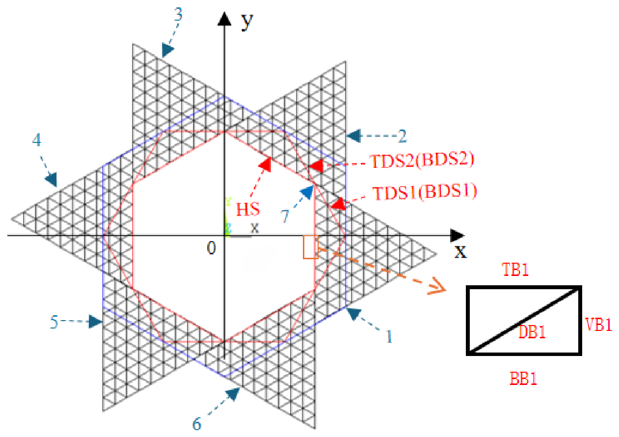
To study the effect of the deployment ratio, parameters such as prestress and structural shape are kept constant across different ratios (see Figure 12), eliminating interfering factors. The cable-truss system drives opening and closing; thus, cable forces are critical to structural stability. Under statically determinate conditions, one hoop cable (HS), two upper diagonal cables (TDS1 and TDS2), and two lower diagonal cables (BDS1 and BDS2) are selected to analyze the relationship between cable force and deployment ratio. Similarly, one upper chord, one diagonal, one lower chord, and one vertical member within the orange dashed box are selected to examine member axial force versus deployment ratio.

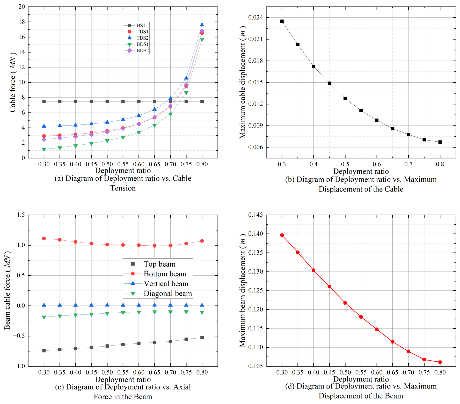
Figure 13b,d shows that as the deployment ratio increases, the structural stiffness increases, and the maximum displacements of both the overall structure and the cable system decrease monotonically, with the absolute slopes of the curves gradually decreasing.

As shown in Figure 13a, the axial force in the hoop cable remains nearly constant, whereas the forces in all diagonal cables increase with the deployment ratio at an increasing rate, exhibiting a trend similar to that of the prestress variation.

As shown in Figure 13c, unlike cable elements, truss beams can sustain compression (internal force $<0$). The vertical member exhibits the smallest absolute internal force, which remains almost unchanged as the deployment ratio increases. Upper chord and diagonal members exhibit negative forces (compression), while the lower chord is positive (tension), consistent with downward bending moment. The absolute internal force in the upper chord decreases with deployment ratio because the slider moves closer to the selected beam, causing the adjacent outer frame to bear more external load.

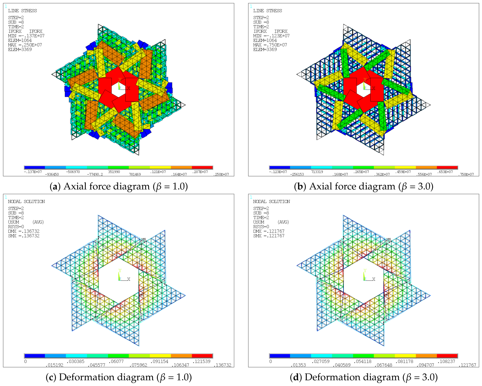
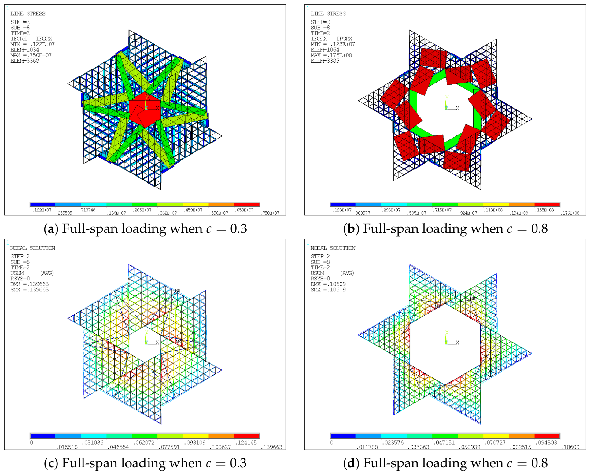
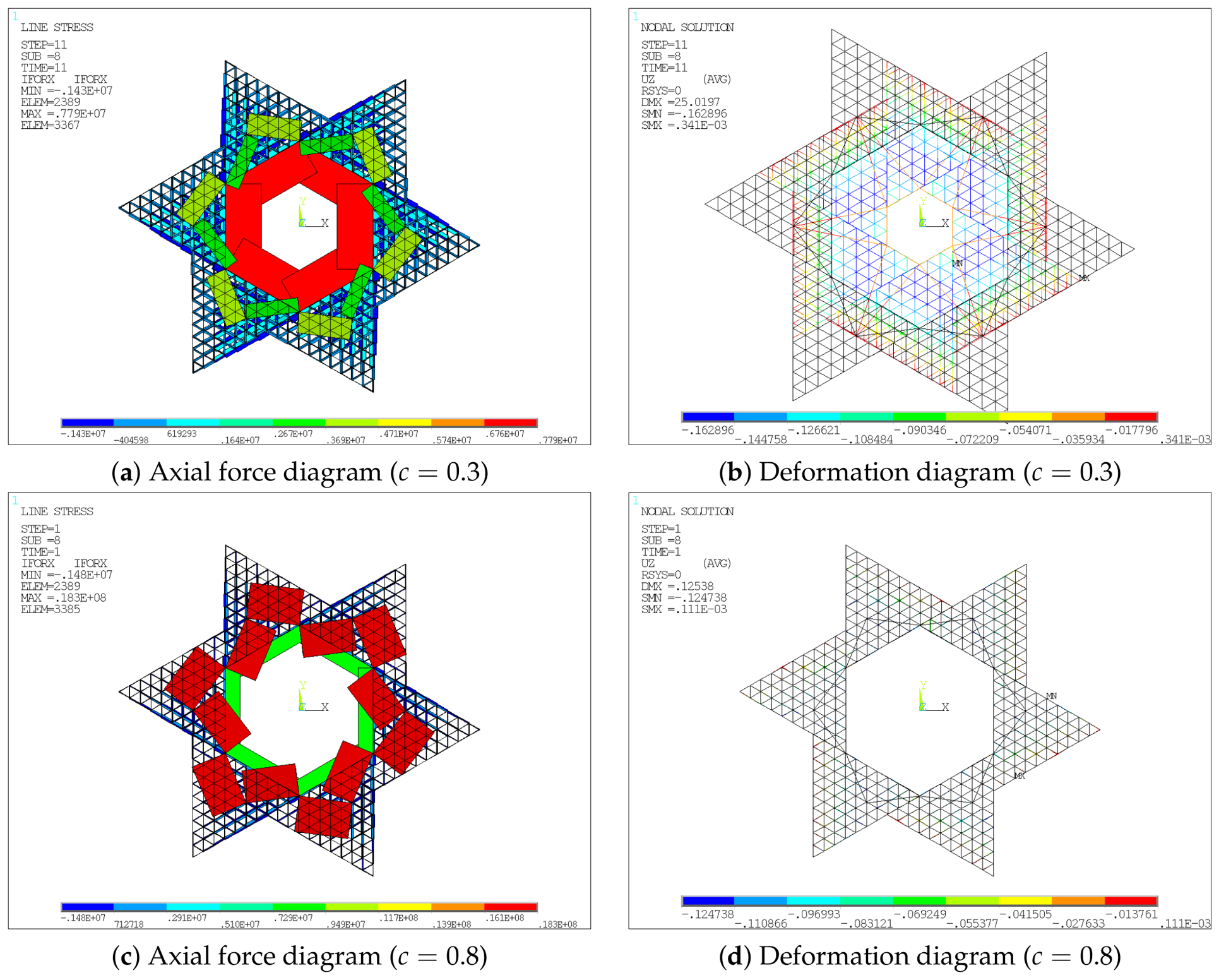
As a supplement to Figure 13a–d, Figure 14 shows axial force and deformation at two extreme deployment ratios ($c=0.3$ and $c=0.8$). At $c=0.3$, the structure is more flexible, with larger deformations and a smaller difference between diagonal cable forces and truss beam forces. At $c=0.8$, stiffness is greater, displacement smaller, and the force difference larger. These contour plots agree with the previous curves, confirming the influence of deployment ratio on structural stiffness and internal forces.

3.3.2. Parametric Analysis of the Influence of Prestress on Structural Performance

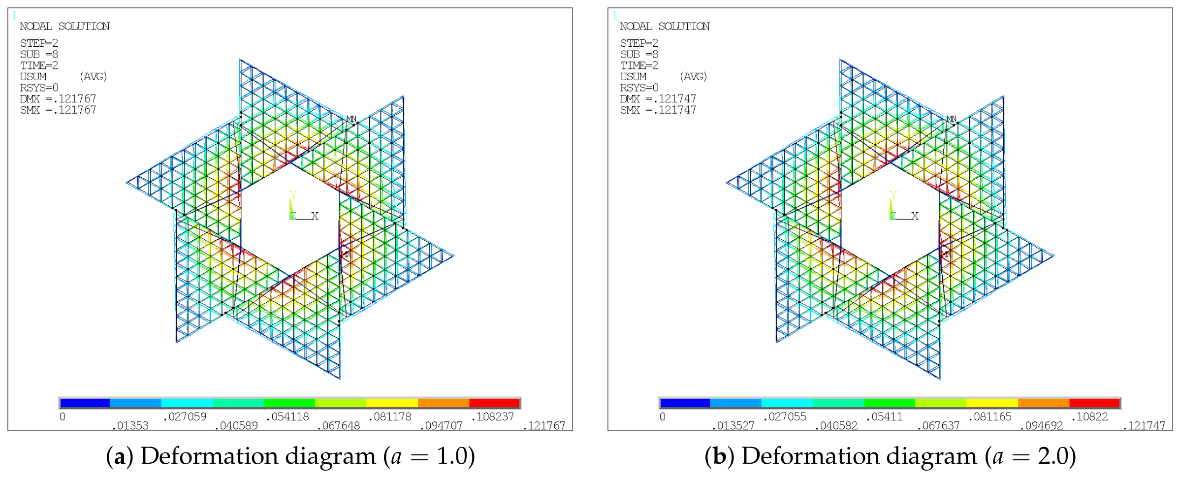
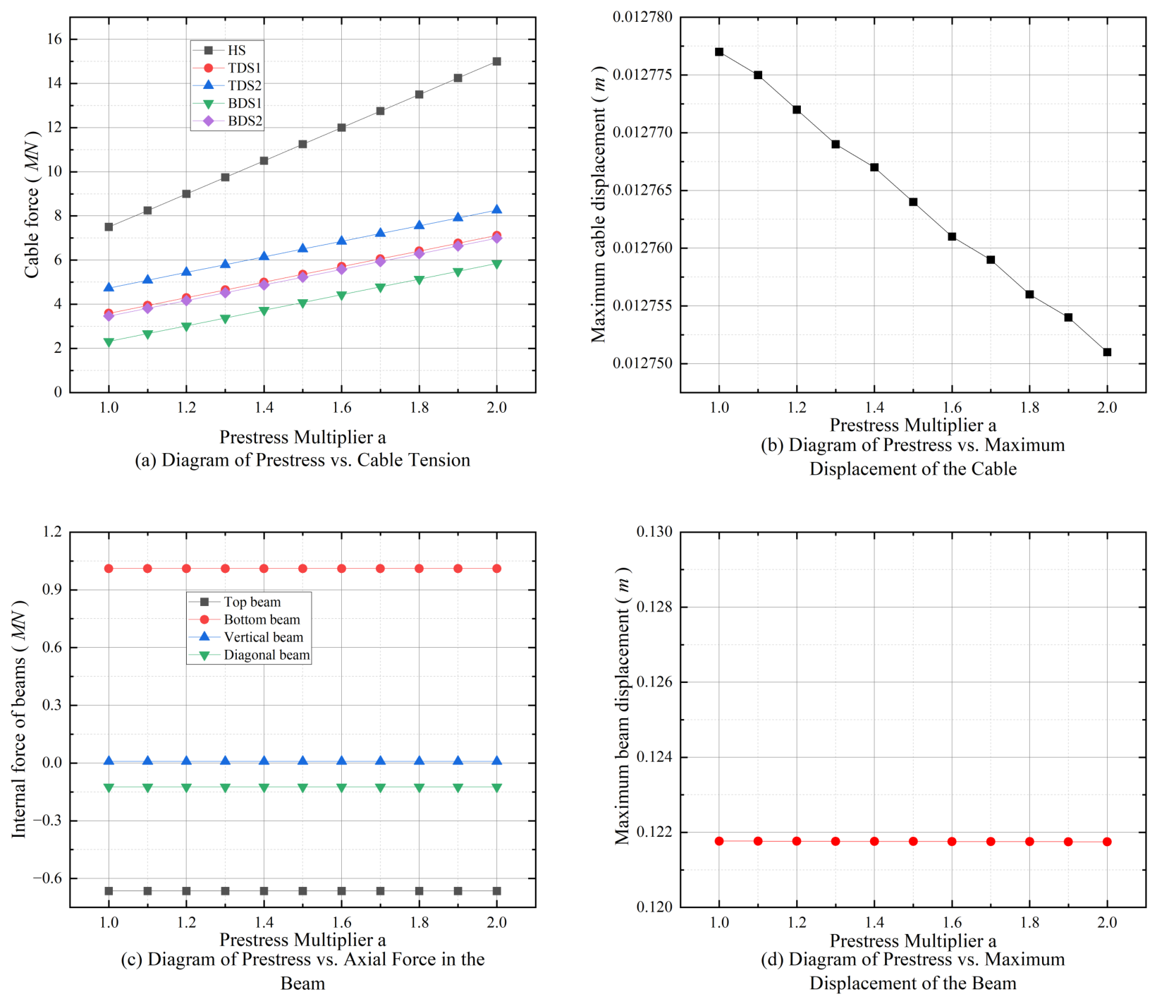
Based on the prestress values mentioned above, the prestress values of the diagonal cables and the hoop cable are multiplied by the same factor a, where a ranges from 1.0 to 2.0 in increments of 0.1. The data are extracted at each increment.

Figure 15a shows that as the prestress multiplication factor increases, the internal forces in the hoop cable and diagonal cables increase linearly, and the difference between them becomes larger. This indicates that the hoop cable is more sensitive to prestress changes than the diagonal cables.

As shown in Figure 15b,d, as the prestress multiplication factor increases, the maximum displacements of both the cable-truss structure and the overall structure remain almost unchanged. This is because the displacement is mainly influenced by self-weight, external loads, and structural geometric parameters.

As shown in Figure 15c, the effect of prestress on the axial forces of the reciprocal truss is negligible. Therefore, when the structural deformation meets the design requirements but negative cable forces occur, the problem can be addressed by increasing the cable prestress without changing the geometry of the structure or its members and without causing significant additional deformation.

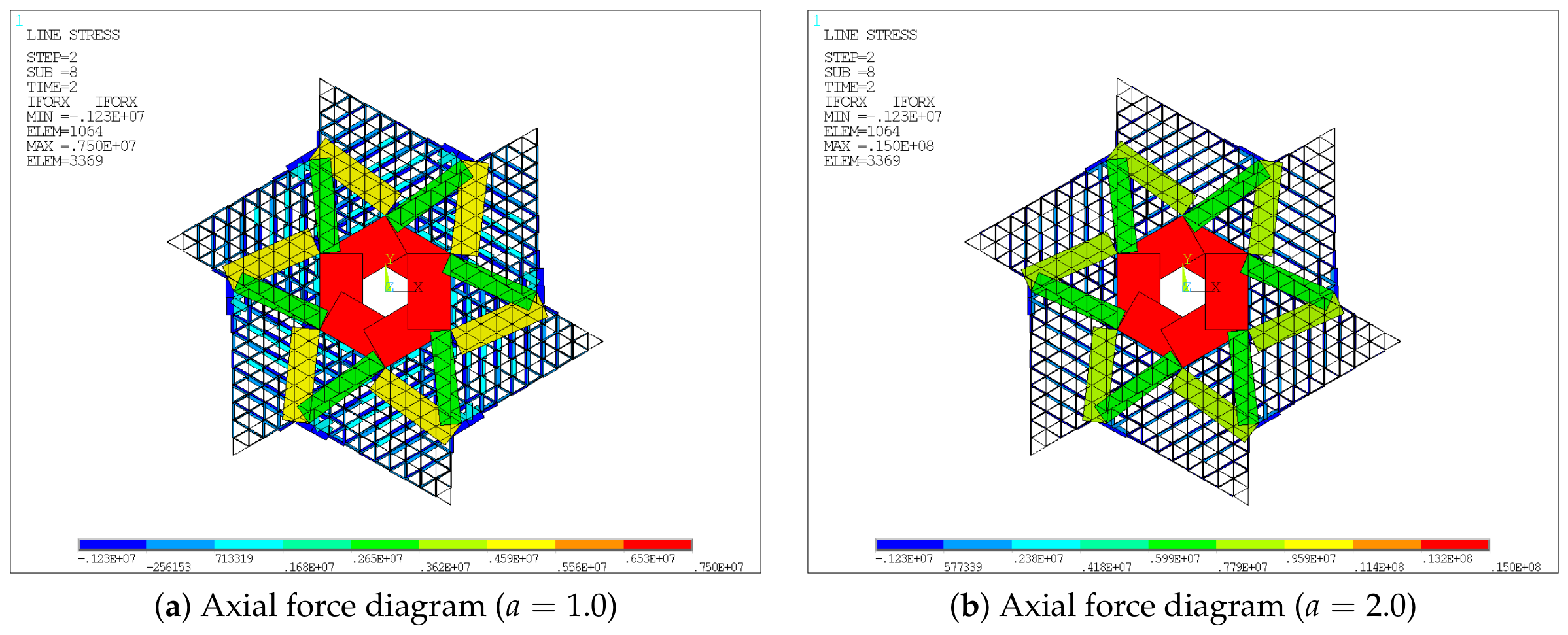
As a supplement to Figure 15a–d, Figure 16 and Figure 17 present the axial force and deformation distributions at two representative prestress levels ($a=1.0$ and $a=2.0$). The deformation contours in Figure 17c,d are consistent with the earlier observation that the overall structural displacement remains nearly unchanged as the prestress increases. Meanwhile, the axial force diagrams in Figure 16a,b show that higher prestress increases cable tension while keeping the beam internal forces almost constant. This indicates that prestress mainly affects cable forces without significantly changing the internal forces of the truss members or the structural stiffness.

3.3.3. Parametric Analysis of Beam Section Depth

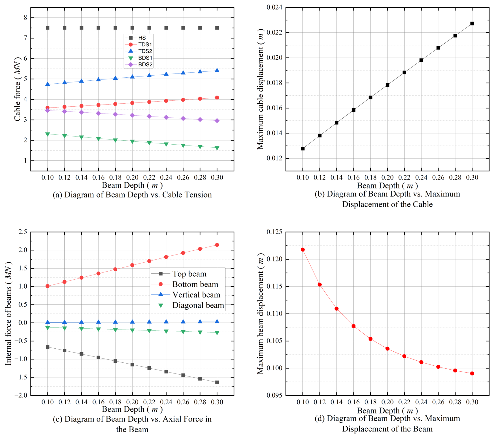
In this subsection, the influence of the beam section depth in the reciprocal truss structure is analyzed. The beam section width and thickness remain constant, while the beam section depth ranges from $0.1\mathrm{m}$ to $0.3\mathrm{m}$, with data extracted at increments of $0.02\mathrm{m}$.

The deformation can be explained using the truss deflection formula ${\delta }_1\propto {\displaystyle \frac{q{L}^4}{E{I}_{eq}}}$, where $I_{eq}\propto A{h}_0^2$, $h_0$ is the distance from the centroid of the upper and lower beams to the centroidal axis of the truss, and A is the sum of the cross-sectional areas of the truss beams. Therefore, as the beam section depth increases, the flexural stiffness of the beam increases significantly, thereby reducing the deformation of the structure under vertical load. Since both the external load and the self-weight of this structure act in the vertical direction, the maximum beam displacement decreases.

As shown in Figure 18d, as the beam section depth increases, the maximum beam displacement decreases at a diminishing rate. In contrast, Figure 18b shows that the maximum displacement of the cable elements increases linearly with beam section depth, because beam self-weight increases linearly, raising the vertical downward load on the cable-truss structure.

As shown in Figure 18a, as the beam section depth increases, the self-weight of the reciprocal truss increases accordingly. Since the hoop cable is a transverse member mainly subjected to lateral loads and lateral displacements, the hoop cable force remains almost unchanged. In contrast, because the diagonal cables carry both lateral and vertical loads, the axial force in the upper diagonal cables increases, while that in the bottom diagonal cables decreases.

As shown in Figure 18c, as the beam section depth increases linearly, the bending moment of the structure also increases linearly. This leads to a linear increase in the axial forces of the top and bottom chords. The compressive force in the diagonal members gradually increases, while the axial force in the vertical members is negligible compared with those in the top and bottom chords.

As a supplement to Figure 18a–d, Figure 19 shows axial force and deformation at two beam depths ($h=0.1\mathrm{m}$ and $h=0.3\mathrm{m}$). The deformation diagrams (Figure 19c,d) confirm that increasing the beam depth reduces maximum displacement due to higher flexural stiffness. The axial force diagrams (Figure 19a,b) show increased top chord compression and bottom chord tension, along with altered diagonal cable force distributions. These visualizations align with the trends in Figure 18.

Therefore, in structural design and optimization, increasing the beam section depth only slightly reduces structural deformation but may worsen the force conditions in the diagonal cables, because the lower diagonal cables may be in compression. For this reason, this approach is not recommended as a primary means of increasing stiffness. Conversely, if the maximum displacement of the structure is far below the allowable value and some internal forces in the cable-truss structure are unsatisfactory, reducing the beam section depth can be a feasible solution.

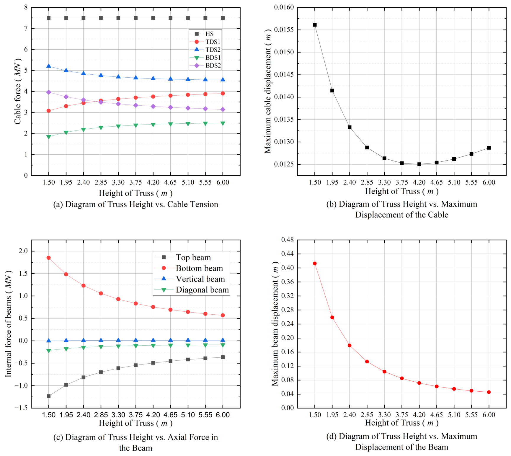
3.3.4. Parametric Analysis of Truss Height

In this subsection, the influence of the truss height of the reciprocal truss structure is analyzed. The truss height ranges from $1.5\mathrm{m}$ to $6.0\mathrm{m}$, with data extracted at increments of $0.45\mathrm{m}$. The results are plotted in Figure 20.

Figure 20d shows that as the truss height increases, the maximum beam displacement decreases, and the absolute slope of the curve gradually diminishes. However, compared with increasing the beam section depth, increasing the overall truss height has a much more significant influence on the structural stiffness, as indicated by the formula ${\delta }_1\propto {\displaystyle \frac{q{L}^4}{E{I}_{eq}}}$ in the previous subsection.

Figure 20a shows that as the truss height increases, the hoop cable force remains nearly unchanged because it primarily bears lateral loads. Structural stiffness improves, maximum displacement decreases, and the structure approaches a more favorable stress state. Consequently, internal forces in cables of the same type converge and stabilize. As truss height has little effect on self-weight, total internal force changes only slightly. Given the allowable maximum displacement of $0.20\mathrm{m}$, the truss height should be no less than $2.40\mathrm{m}$.

As shown in Figure 20c, as the truss height increases linearly, the absolute axial forces in the top and bottom chords decrease at a diminishing rate. This occurs because self-weight and external load remain unchanged, so bending moment is constant, giving $N\propto M/h$. Meanwhile, the angle between diagonal members and the chords increases, reducing the absolute axial force in diagonals ($N\propto V$/$\sin \theta$).

As shown in Figure 20b, as the truss height increases, the maximum displacement of the cable-truss structure first decreases and then increases. This is because, as the truss height increases, the cable-truss structure approaches an ideal stress state, causing its vertical displacement to decrease continuously. When the truss height approaches $4.2\mathrm{m}$, although the vertical displacement continues to decrease, the reduction becomes smaller. In contrast, as the truss height increases, the truss displacement of the cable-truss structure increases. Consequently, the maximum displacement of the cable-truss structure first decreases and then increases.

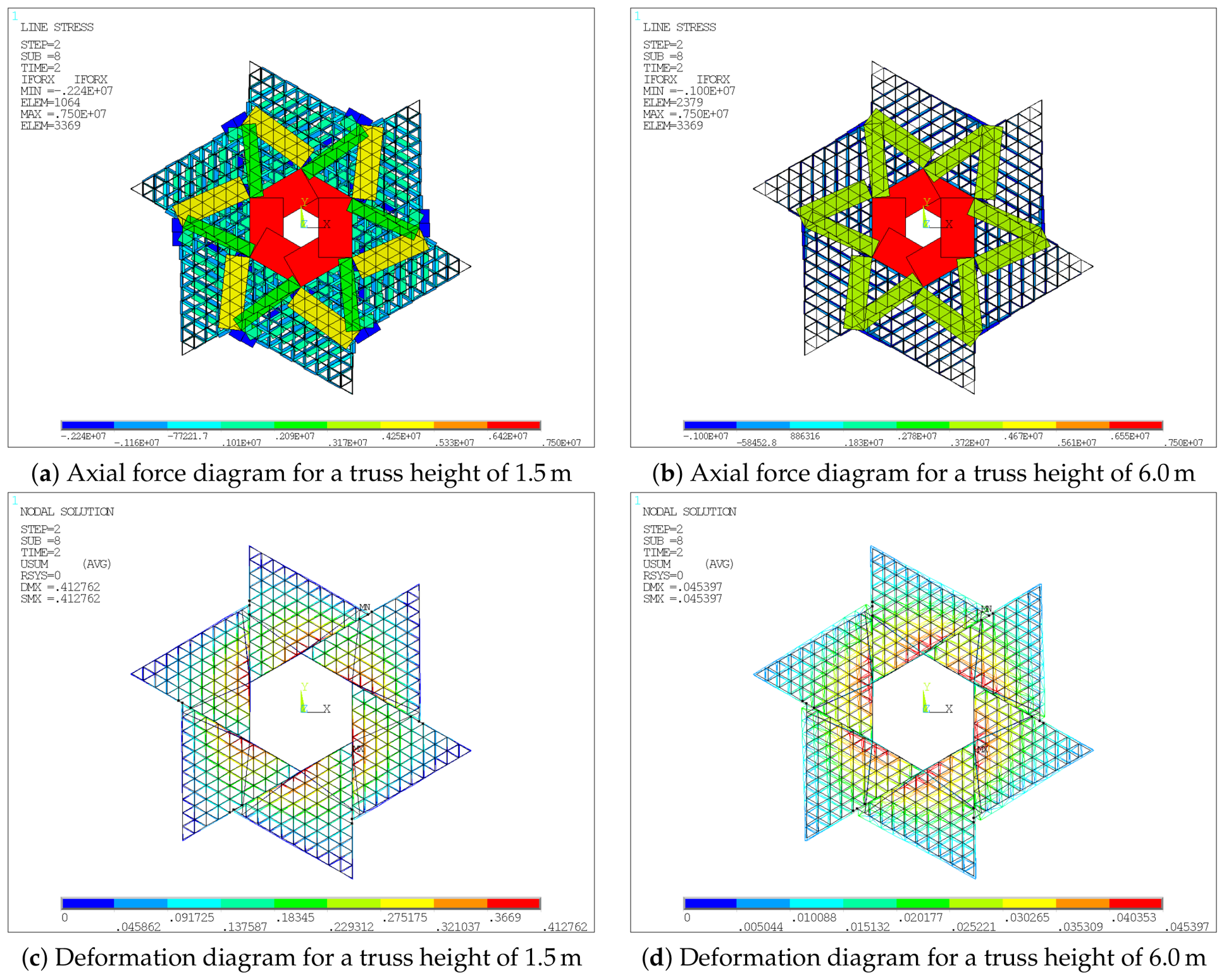
As a supplement to Figure 20a–d, Figure 21 presents the axial force and deformation distributions at truss heights of $1.5\mathrm{m}$ and $6.0\mathrm{m}$. The deformation diagrams in Figure 21c,d are consistent with the observation that increasing the truss height significantly reduces structural displacement, reflecting the improvement in flexural stiffness. Meanwhile, the axial force diagrams in Figure 21a,b show the reduction in chord and diagonal member forces as well as the convergence of cable tensions, which is consistent with the trends observed earlier. These visualizations indicate that a larger truss height leads to a stiffer structure with a more balanced internal force distribution.

In summary, when the maximum displacement of the structure substantially exceeds the allowable limit, increasing the beam depth may cause secondary cable-force issues. In contrast, increasing truss height balances diagonal cable forces (reducing such issues), minimally increases self-weight, and greatly reduces displacement. Therefore, increasing truss height is more efficient and economical.

3.3.5. Parametric Analysis of Cable Cross-Sectional Area

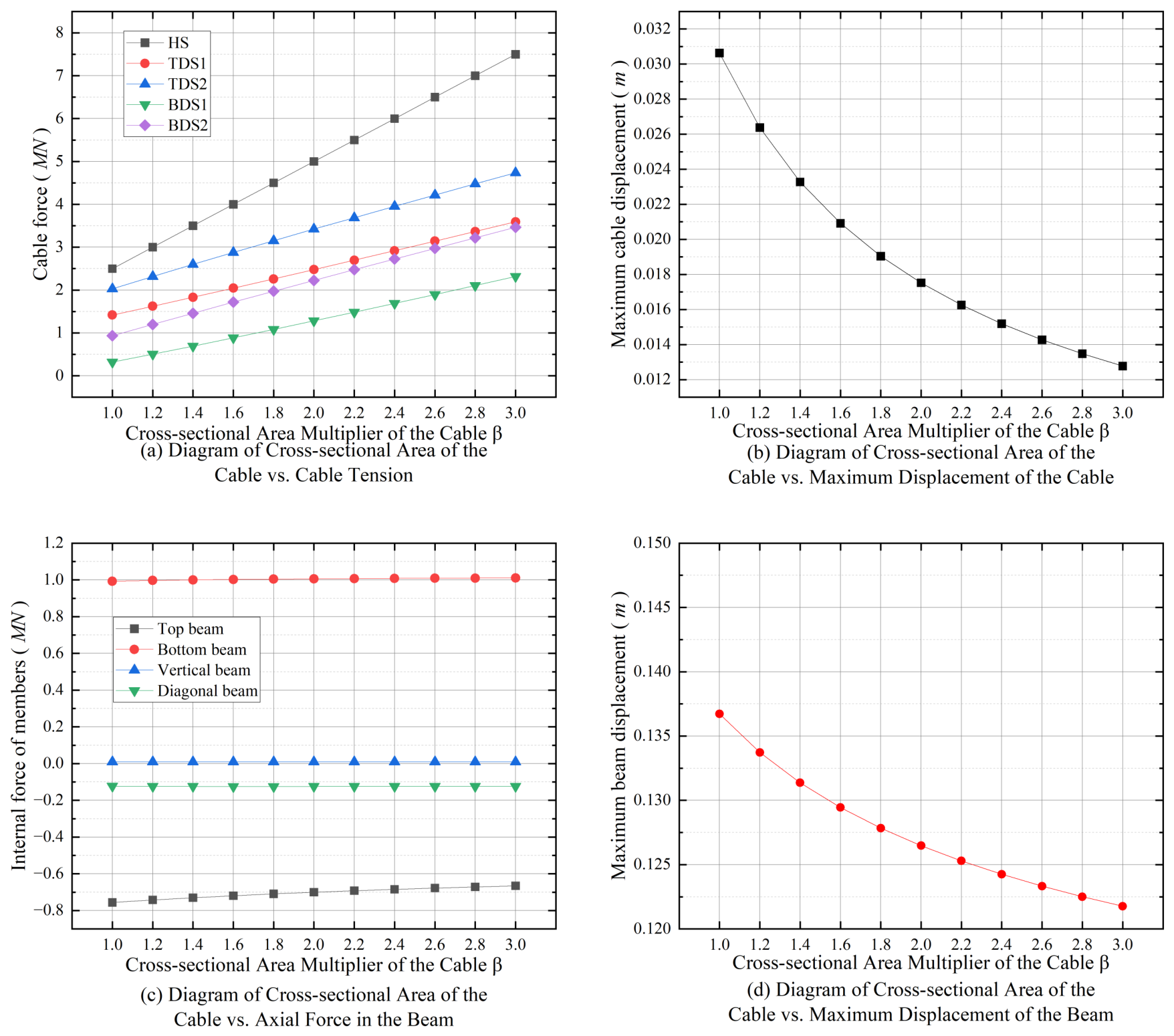
As shown in Figure 22, using a cable cross-sectional area of $0.007238229{\mathrm{m}}^2$ as the reference value (a single cable with a radius of $4.8\mathrm{cm}$), the cross-sectional areas of the hoop cable and diagonal cables are both multiplied by the same factor $\beta$ to analyze the influence of cable cross-sectional area on the mechanical performance of the structure.

As shown in Figure 22d, as the cable cross-sectional area multiplier $\beta$ increases, the maximum structural displacement decreases with a diminishing slope. This occurs because the maximum displacement is primarily vertical, accommodated by cables. As axial members, cable deformation follows Hooke’s law, giving a negative correlation between displacement and area. Prestress has negligible effect on displacement. Thus, increasing cable area yields the inverse proportionality curve in Figure 22d; the same reasoning applies to Figure 22b.

Figure 22a shows that under constant prestress, as $\beta$ increases, hoop and diagonal cable forces increase approximately linearly. At $\beta =1.0$, bottom diagonal cable BDS1 becomes negative (compression), violating tension-only behavior. To ensure all cables remain in tension, $\beta =3.0$ is recommended.

Figure 22c shows that as the cable cross-sectional area multiplier increases, axial forces in vertical members, diagonal members, and bottom chords remain nearly unchanged. In contrast, the absolute top chord axial force decreases at a diminishing rate, due to internal force redistribution from reduced structural deformation.

As a supplement to Figure 22a–d, Figure 23 shows axial force and deformation at $\beta =1.0$ and $\beta =3.0$. The deformation diagrams (Figure 23c,d) confirm that increasing the cable area reduces displacement. The axial force diagrams (Figure 23a,b) show increased cable tension and reduced top chord compression. These visualizations indicate that a larger cable area improves both stiffness and cable force conditions.

Based on the above observations, increasing the cable area may be considered when the maximum displacement slightly exceeds the allowable value, cable tension is too low or negative, or cable tensile stress approaches its limit. Such an increase enhances sectional stiffness and cable force conditions, ensuring stability and normal serviceability during opening and closing.

In summary, the retractable cable-driven reciprocal truss structure uses the high stiffness of the reciprocal truss system to resist vertical loads and self-weight, thereby exhibiting strong resistance to deformation. At the same time, it takes advantage of the lightweight and high-strength properties of the cable-truss system by replacing independent cables with continuous cables and arranging sliding units on the reciprocal truss. This greatly reduces the number of actuators and the complexity of the retraction mechanism. Furthermore, parametric analysis enables the structure to be specifically optimized for different spans, loading conditions, and functional requirements. Finally, the separation of driving and load-bearing functions clarifies the load transfer mechanism. The cable-truss system is primarily responsible for driving the opening and closing motion and transmitting part of the vertical load, while the reciprocal truss and triangular panels mainly provide load-bearing capacity, stiffness, and enclosure functions. This functional separation results in a clear force path, facilitating analysis and design.

4. Analysis of the Opening and Closing Motion of the Structure

This section presents a static analysis of the opening and closing processes of the structure using ANSYS APDL, based on the model established in Section 3. Specifically, the opening and closing processes are simulated through static analysis, and the results are compared with those of the full-span load case in the nonlinear static analysis of the structure from the Section 3.3.1. In addition, the prestress and displacement conditions are compared with those in Section 2 to verify whether the structure maintains good mechanical performance during opening and closing. Furthermore, engineering strain, Green–Lagrange strain, and logarithmic strain are adopted separately to adjust the cable elements during the opening and closing process. Form-finding and force-finding analyses are also carried out for the hoop cables during the closing process. Finally, among the three strain formulations, the most theoretically appropriate cable-length adjustment method is identified.

4.1. Analysis of the Initial Equilibrium State

For a clearer comparative analysis, this subsection adopts the same analysis method as that used in the motion path analysis in Section 2. Three key structural nodes, namely, Node 10, Node 19, and Node 25, as shown in Figure 2a, are selected for the comparative analysis of nodal coordinates.

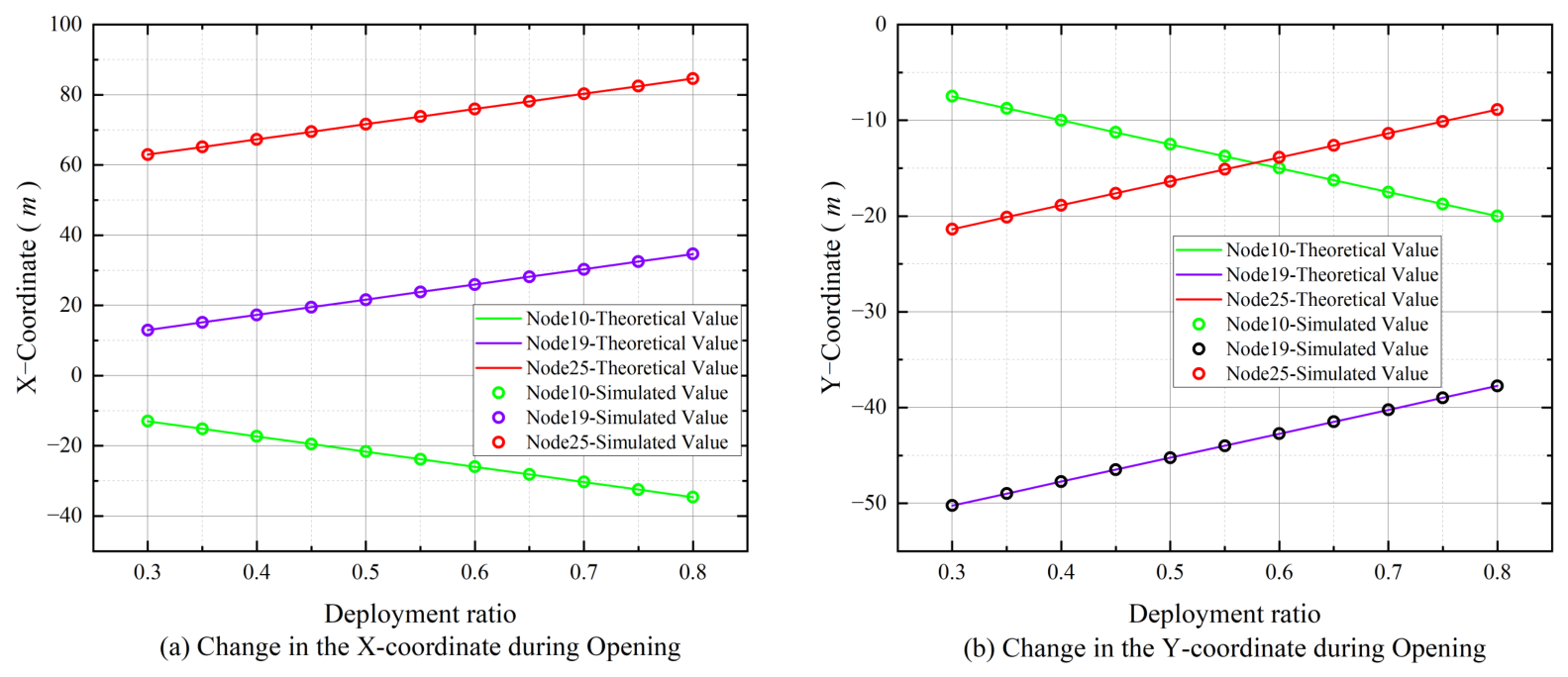
Based on the variation curves of nodal coordinates presented in Figure 24, it can be observed that under different deployment ratios, the theoretical and simulated X- and Y-coordinates of the three selected key nodes are approximately equal, and the curves are essentially coincident. This indicates that during the simulation of structural opening and closing, the simulated nodal displacements closely match the theoretically expected motion trajectories, with the errors remaining within an acceptable range. Consequently, the finite element model established in ANSYS APDL can satisfactorily reproduce the ideal motion trajectory of the structure without introducing significant computational errors due to the application of prestress.

To investigate the mechanical performance of the structural model in the initial equilibrium state under prestress, neither external loads nor self-weight are included in the calculation; only prestress is considered. Under these conditions, among the three types of cables, namely, hoop cables, upper diagonal cables, and bottom diagonal cables, the internal forces and geometric lengths of cables of the same type are identical. This is due to the symmetry of the structure and the symmetric application of prestress. Furthermore, because only prestress is considered and the upper and bottom diagonal cables are symmetric about the plane of the hoop cable, the internal forces and lengths of the upper and bottom diagonal cables are equal. Based on the above, to simplify the analysis, this subsection selects only the hoop cable and diagonal cables for a comparative analysis of the theoretical and simulated values, focusing on the deviations in cable internal force and geometric length under the two conditions.

As shown in Figure 25b, under different deployment ratio values, the theoretical and simulated lengths of each cable are in good agreement, and the curves for each cable are essentially consistent. The hoop cable length increases linearly, while the diagonal cable lengths decrease monotonically.

However, compared with the cable length variation graph, the cable force variation graph shown in Figure 25a shows certain discrepancies. It should be noted that this opening and closing simulation analysis starts from a deployment ratio of $c=0.8$ for the closing process. The simulated and theoretical values are in good agreement at the first three deployment ratio values, indicating that at the beginning, the structure can satisfactorily reproduce the theoretical force condition. However, as the structure continues to close, starting from a deployment ratio of $c=0.65$, the cable force values begin to deviate more noticeably. Because there remains a difference between the theoretical and simulated displacements of the structure, discrepancies between the theoretical and simulated cable forces arise during the subsequent closing process. Since these discrepancies are not large, the cable force values remain within a reasonable range.

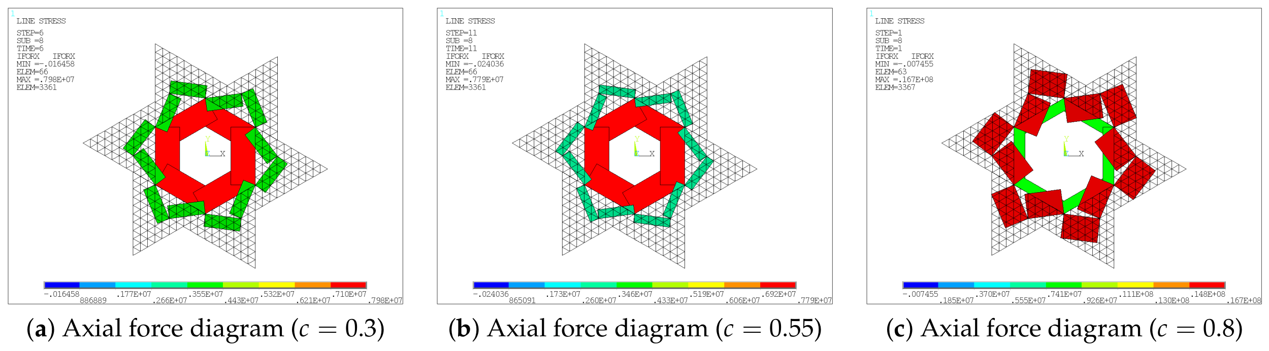
As shown in Figure 26, as the deployment ratio increases, the hoop cable force remains nearly unchanged, the diagonal cable force increases continuously, while the force in the reciprocal truss remains zero throughout.

4.2. Nonlinear Pseudo-Static Analysis of Opening and Closing

This subsection presents a nonlinear analysis of the opening and closing processes. In this analysis, in addition to prestress, the self-weight of the structure and the live load on the non-walkable roof are also considered.

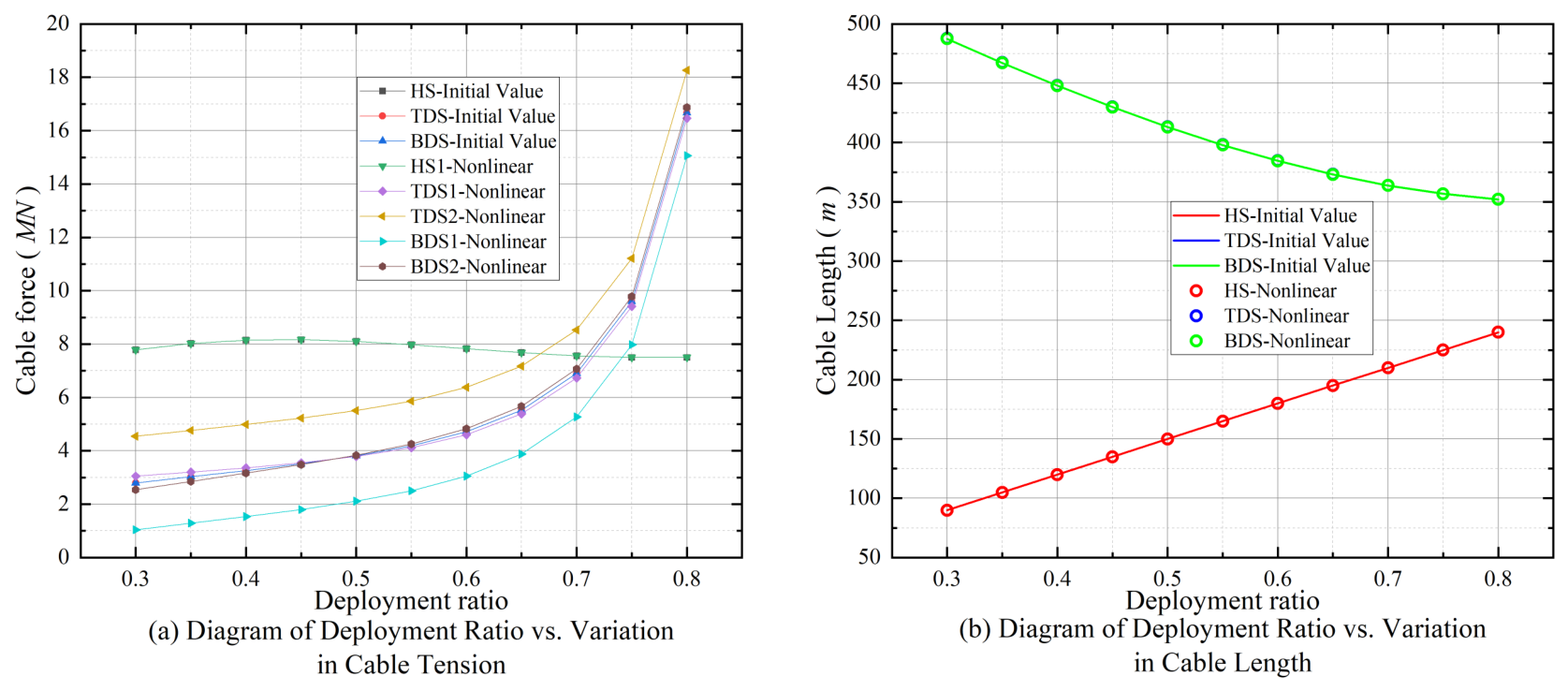
As shown in Figure 27b, due to the high overall stiffness of the structure, the displacements induced by self-weight and external loads are negligibly small compared with the large displacements caused by structural opening and closing. Therefore, even when self-weight and external loads are included, the relationship curve between the deployment ratio and cable length obtained from the nonlinear static analysis almost coincides with that from the initial equilibrium analysis under prestress alone, i.e., it nearly coincides with the theoretical cable length. This indirectly demonstrates that the overall stiffness of the structure is sufficiently high, so the influence of external loads and self-weight on structural displacements can be ignored.

In Figure 27a, compared with the values obtained from the initial equilibrium analysis under prestress alone, the values from the nonlinear analysis show very little change. Since the self-weight and external loads act in the Z-direction, they are primarily carried by the diagonal cables in the cable-truss structure. Meanwhile, as the deployment ratio increases, the difference between the internal forces in diagonal cables TDS1 and TDS2 increases, and the same trend is observed for diagonal cables BDS1 and BDS2. As a result, the internal force in TDS1, which is initially greater than that in BDS2, gradually becomes smaller than that in BDS2. Furthermore, the growth curves of the cable forces are similar. In summary, the nonlinear analysis results further show that, owing to the extremely high overall stiffness of the structure, the effects of self-weight and external loads on cable length are minimal. However, the cable forces differ due to internal force redistribution induced by the application of self-weight and external loads.

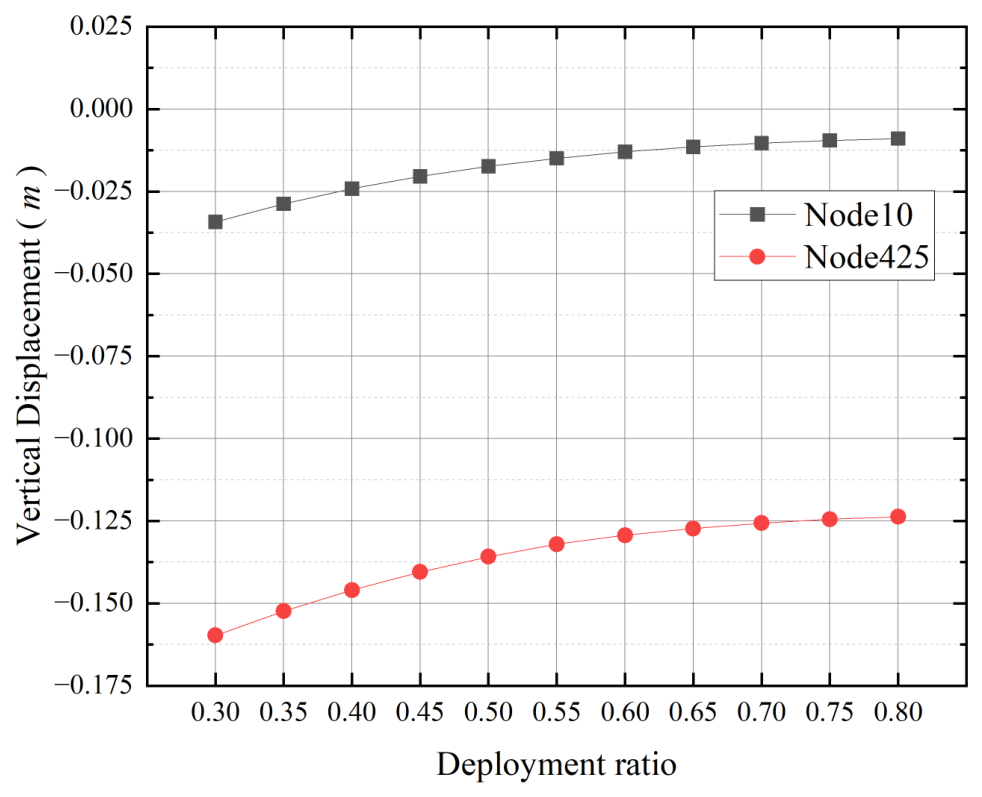
Two nodes, ring Node 10 and truss Node 425, are selected to plot their vertical displacements during the closing process of the structure. The horizontal coordinates of Node 425 are defined as the midpoint coordinates of Node 7 and Node 19, with the Z-coordinate set to $-3\mathrm{m}$. The coordinates of Node 7 are as follows:

$$\left[\begin{array}{c}{x}_7\hfill \\ y_7\hfill \\ z_7\hfill \end{array}\right]={\left[\begin{array}{ccc}\cos \alpha & -\sin \alpha & 0\\ \sin \alpha & \cos \alpha & 0\\ 0& 0& 1\end{array}\right]}^0\left[\begin{array}{ccc}\cos (\pi /6)& -\sin (\pi /6)& 0\\ \sin (\pi /6)& \cos (\pi /6)& 0\\ 0& 0& 1\end{array}\right]\left[\begin{array}{c}cR\\ 0\\ 0\end{array}\right]$$

(23)

The coordinates of Node 19 are given in Equation (13); thus, the coordinates of Node 425 are as follows:

$$\left[\begin{array}{c}{x}_{425}\\ y_{425}\\ z_{425}\end{array}\right]=\left[\begin{array}{c}{x}_7+0.5\times \left(x_{19}-x_7\right)\\ y_7+0.5\times \left(y_{19}-y_7\right)\\ -3\end{array}\right]$$

(24)

As shown in Figure 28, as the deployment ratio increases, the absolute value of the vertical displacement of the nodes decreases monotonically, and the rate of decrease gradually diminishes. This indicates that the overall stiffness of the structure increases with the deployment ratio. This is because, as the deployment ratio increases, the minimum angle between the diagonal cables and the horizontal plane gradually becomes larger, and the contribution of the cable-truss stiffness to the overall structure progressively increases. Consequently, the absolute value of the vertical displacement of the nodes continuously decreases.

As shown in Figure 29, the deformation distributions during structural closure remain regular, while the vertical displacement of the structure remains small. These results indicate that the opening and closing motion of the structure can be realized by adjusting the cable length. Correspondingly, the axial force in the hoop cable exhibits only small variations. This differs from the results of the deployment ratio analysis under different loading conditions presented in Section 3.

Since the structure is retractable, it can be assembled in the fully opened state, thereby eliminating the need for extensive scaffolding support underneath the large-span structure. After the assembly is completed, the scaffolding can be removed, and the structure can be operated directly for opening and closing.

4.3. Cable-Length Adjustment Method in ANSYS APDL Software

In ANSYS APDL, temperature loads and prestress methods are commonly used to adjust member lengths, with strain-based approaches primarily used to determine the required temperature loads and prestress values. The three main methods for calculating strain are engineering strain, Green–Lagrange strain, and logarithmic strain. Among these, engineering strain [46] is the simplest and is mainly used for small-deformation cases; Green–Lagrange strain [47] is more suitable for large-deformation cases; and logarithmic strain is primarily used for plastic deformation studies [48] and for investigating the true constitutive relationship of materials [49]. In this subsection, the three strain calculation methods are used to determine the temperature load values applied to the cable elements to adjust the shape of the cable-truss structure. Form-finding and force-finding analyses are carried out on the structure, and the most theoretically appropriate cable-length adjustment method is identified.

Before the analysis is performed, the formulas for the three methods are introduced. In the present structure, the members whose lengths need to be adjusted are one-dimensional cable members. Therefore, the engineering strain is given by ${\epsilon }_1={\displaystyle \frac{l-l_0}{l_0}}$, the Green–Lagrange strain is given by ${\epsilon }_1={\displaystyle \frac{l^2-l_0^2}{2l_0^2}}$, and the logarithmic strain is given by ${\epsilon }_1=\ln \left({\displaystyle \frac{l}{l_0}}\right)$, where l is the deformed length of the member and $l_0$ is the original length.

In this subsection, the prestress of the hoop cable is set as the load $t=7.5\mathrm{MN}$ divided by the cross-sectional area of the cable element. Accordingly, the strain induced by the applied temperature load is given by ${\epsilon }_2={\epsilon }_1+{\displaystyle \frac{t}{EA}}$. Similarly, the prestress and the corresponding strain ${\epsilon }_2$ for the diagonal cables can be obtained.

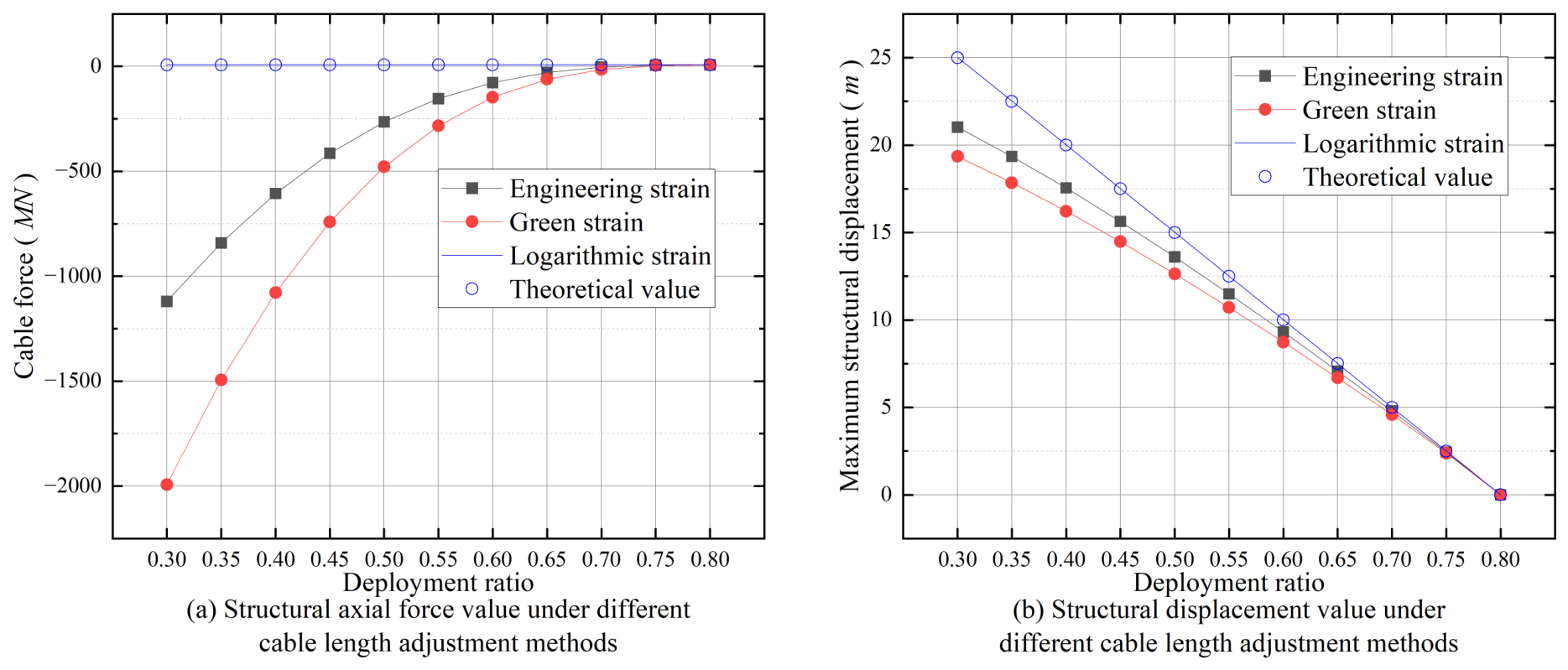
As shown in Figure 30a, as the deployment ratio decreases, the differences between the structural displacement values obtained by adjusting the cable length using engineering strain and Green–Lagrange strain and the theoretical values increase progressively. The deviations obtained using Green–Lagrange strain are larger than those obtained using engineering strain. In contrast, the structural displacement values obtained using logarithmic strain are very close to the theoretical values. This indicates that among the strain-based cable-length adjustment methods, logarithmic strain has the highest feasibility.

Figure 30b further shows that as the deployment ratio decreases, the differences between the axial force values of the hoop cable obtained using engineering strain and Green–Lagrange strain and the theoretical values increase monotonically, with an increasing rate of change. The differences obtained using Green–Lagrange strain remain larger than those obtained using engineering strain. Conversely, logarithmic strain again yields values close to the theoretical values. This further demonstrates the feasibility of using logarithmic strain for cable length adjustment.

Therefore, among the methods for adjusting cable length during structural opening and closing, logarithmic strain provides the highest accuracy, followed by engineering strain, while Green–Lagrange strain is the least accurate. The results in Figure 30b also indicate that, compared with logarithmic strain, Green–Lagrange strain and engineering strain are not suitable for cable length adjustment.

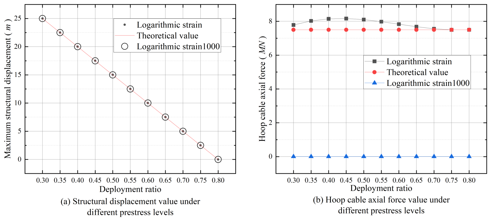
In the previous section, it was determined that logarithmic strain is the only feasible method among the three strain-based approaches for cable-length adjustment. Nevertheless, the accuracy of the adjustment method still requires further investigation. To this end, an additional case is considered in which the prestress of the hoop cable is equivalent to a load of $t=1000\mathrm{N}$ divided by the cross-sectional area of the cable element, and logarithmic strain is adopted for cable-length adjustment. This case is denoted as “Logarithmic strain 1000”. It is then compared with the previous logarithmic strain data and the theoretical values to verify the influence of the prestress magnitude on the accuracy of the adjustment method.

As shown in Figure 31b, even when logarithmic strain is used for cable-length adjustment, a discrepancy remains between the axial force values of the hoop cable and the theoretical values. Meanwhile, as shown in Figure 31a, although the prestress value varies, the structural displacement values remain close to the theoretical values.

For a more precise analysis,

Table 2. Structural displacement under logarithmic strain adjustment.

Deployment Ratio	Logarithmic Strain (m)	Logarithmic Strain 1000 (m)	Theoretical Value (m)
0.8	0	0	0
0.75	2.50396	2.5	2.5
0.7	5.00692	5	5
0.65	7.50915	7.5	7.5
0.6	10.0109	10	10
0.55	12.5124	12.5	12.5
0.5	15.0136	15	15
0.45	17.5146	17.5	17.5
0.4	20.0153	20	20
0.35	22.5156	22.5	22.5
0.3	25.0154	25	25

is presented. As shown in the table, when the prestress corresponding to the logarithmic strain is equivalent to a load of $t=7.5\mathrm{MN}$ divided by the cross-sectional area of the cable element, the structural displacement values deviate from the theoretical values. However, when the prestress corresponding to the logarithmic strain is reduced to $1/7500$ of the previous value, the structural displacement values become very close to the theoretical values, and the values calculated by the software are equal to the theoretical values. Thus, in ANSYS APDL, although the structural opening and closing motion simulated by adjusting the cable length using logarithmic strain is highly accurate, a very small error still exists, and this error increases as the prestress value increases. Nevertheless, the resulting error in the structural displacement values remains small (<1%).

As shown in

Table 3. Axial force of the hoop cable under logarithmic strain adjustment.

Deployment Ratio	Logarithmic Strain (MN)	Theoretical Value (MN)	$\frac{\mathrm{Simulated}\mathrm{Value}}{\mathrm{Theoretical}\mathrm{Value}}$	Logarithmic Strain 1000 (N)	Theoretical Value (N)	$\frac{\mathrm{Simulated}\mathrm{Value}}{\mathrm{Theoretical}\mathrm{Value}}$
0.8	7.5	7.5	1	1000	1000	1
0.75	7.497113	7.5	0.999615067	996.11	1000	0.99611
0.7	7.561502	7.5	1.008200267	1004.2	1000	1.0042
0.65	7.6827	7.5	1.02436	1021.4	1000	1.0214
0.6	7.8327	7.5	1.04436	1042.7	1000	1.0427
0.55	7.982	7.5	1.064266667	1061.8	1000	1.0618
0.5	8.102221	7.5	1.080296133	1078.5	1000	1.0785
0.45	8.166303	7.5	1.0888404	1086.5	1000	1.0865
0.4	8.148749	7.5	1.086499867	1086.4	1000	1.0864
0.35	8.027312	7.5	1.070308267	1070.5	1000	1.0705
0.3	7.7858	7.5	1.038106667	1038.4	1000	1.0384

, as the prestress increases, the ratio of the simulated axial force of the hoop cable to the theoretical value also increases. However, the deviation of this ratio from unity remains extremely small (<1%). This indicates that although the logarithmic strain method for cable-length adjustment inevitably introduces some error, prestress has only a minor influence on the discrepancy between the simulated and theoretical axial forces of the hoop cable.

In summary, adjusting the cable length using logarithmic strain is a relatively accurate method for achieving structural opening and closing among the strain-based approaches. The error can be neglected provided that the prestress is not increased excessively. Although the influence of the error on the internal forces of the structure is greater than that on the displacements, it remains within an acceptable range (<10%).

In the numerical simulation of the opening and closing motion, the error in nodal displacements is found to be very small, while the error in cable forces is relatively large. This is because the cable-length variation obtained from logarithmic strain can reproduce the structural configuration with high accuracy, although small errors in nodal displacements still exist. Because the material has a large elastic modulus, these small displacement errors can lead to relatively large internal force errors.

5. Conclusions

This paper proposes a retractable cable-driven reciprocal truss structure and presents theoretical analysis and numerical simulations. The main contributions and conclusions are as follows:

(1)

A design method integrating a tensegrity structure with sliding cables and a reciprocal truss structure is proposed. By replacing independent cables with continuous cables and employing the reciprocal truss as the roof structure, the structural complexity, number of actuators, and overall cost are reduced. This provides new ideas for the design of large-span spatial structures.

(2)

A prestress design method for the proposed structure is established. Form-finding analysis, motion path planning, and cable-length adjustment analysis are conducted using ANSYS.

(3)

Modal analysis is performed to obtain the vibration characteristics corresponding to each natural frequency.

(4)

The effects of deployment ratio, external load, prestress, beam section depth, truss height, and cable cross-sectional area on structural stiffness are systematically investigated, leading to an optimized structural configuration. The results show that as the deployment ratio increases, structural stiffness improves and the maximum displacement decreases. The variation in maximum displacement under different loading conditions is minimal (≤1%), and the maximum displacement is proportional to the external load. The maximum displacement satisfies $\delta \propto {\delta }_1+{\delta }_2$, where ${\delta }_1\propto {\displaystyle \frac{q{L}^4}{E{I}_{eq}}}$ and ${\delta }_2\propto {\displaystyle \frac{FL}{EA}}$. Prestress has a negligible effect on the maximum displacement, whereas truss height has the most significant influence. In the force-finding analysis, changes in prestress and cable cross-sectional area lead to a linear increase in cable forces, while other parameters have limited effects on the hoop cable force. This provides a theoretical basis and technical reference for the design, analysis, and optimization of similar cable-driven retractable structures.

(5)

Initial equilibrium analysis and nonlinear analysis are performed using ANSYS. The results indicate that the errors in displacement and cable length are extremely small (≤0.5%), while the cable force errors remain within a small range (≤9%), depending on the cable-length adjustment method. Among the cable-length adjustment methods, the logarithmic strain method yields the smallest error and the highest accuracy, satisfying the adjustment requirements. The finite element displacement results agree well with the theoretical values at low prestress levels, with minor deviations observed at higher prestress levels. In the force-finding analysis, even when the prestress multiplier varies significantly, the deviation between the simulated and theoretical values remains small (≤1%). This provides a theoretical basis for cable-length adjustment in cable-driven structures.