A 3D Laser Scanning and BIM-Based Workflow for Localization and Classification of MEP Pipe Installation Discrepancies

Abstract

Mechanical, electrical, and plumbing (MEP) pipe installation discrepancies can increase rework, complicate inspection, and affect subsequent operation and maintenance. This study presents a 3D laser scanning and Building Information Modeling (BIM)-based workflow for localizing and preliminarily classifying MEP pipe installation discrepancies in a building project. Preprocessed scanned pipe point clouds are registered with BIM-derived pipe point clouds through a coarse-to-fine Scan-BIM registration process. Individual pipe instances are extracted using distance-threshold-based growing, and scan-to-BIM pipe correspondence is established using nearest-neighbor root mean square error (RMSE). Pipes with relatively large overall RMSE values are further divided into slices to identify local high-discrepancy intervals. A slice-level discrepancy distribution function $R\left(s\right)$, together with derivative-magnitude and derivative-fluctuation thresholds, is used to support preliminary Type 1/Type 2 interpretation of representative discrepancy patterns. In a student dormitory case, the workflow screened local pipes with relatively large discrepancies, localized maximum-RMSE regions, and distinguished representative connection-related discrepancies from overall offset or inclination cases. A threshold perturbation check showed consistent Type 1/Type 2 labels for the four representative cases within the tested range. The workflow provides case-study evidence for localized MEP pipe inspection, while broader validation across projects and pipe systems remains necessary.

1. Introduction

In building projects, mechanical, electrical and plumbing (MEP) installation engineering plays a critical role in construction coordination and later operation and maintenance, particularly in projects with dense heating, ventilation, and air conditioning (HVAC), water supply and drainage, power, and communication systems [1,2]. The construction of an MEP system involves the installation of multiple systems in a limited space, which often leads to conflicts and rework. Such installation conflicts and discrepancies are not only cost and quality-control problems; under the broader demand for reducing greenhouse gas emissions in the built environment, they may also cause material waste and additional embodied carbon when pipes, fittings, supports, or related components need to be removed, replaced, or re-installed [3]. In many cases, the discrepancies arising between the installed pipes and the as-designed models can complicate the inspection, maintenance and management of pipes [2]. Therefore, inspecting the installation discrepancies and construction quality of MEP systems is critical and essential. Reliable discrepancy analysis and inspection can support MEP construction quality control, help reduce rework, and improve subsequent inspection and management [4,5].

Currently, the discrepancy analysis and quality inspection of MEP systems are often performed by on-site safety officers using tape measures, spirit levels, and other manual devices. Although such methods are easy to implement and remain necessary for engineering judgment, they are labor-intensive, depend on inspectors’ experience, and usually provide only sparse measurements at selected positions. As a result, it is difficult to obtain continuous three-dimensional discrepancy information for complex and densely arranged MEP pipe layouts. This limitation becomes more evident in large-scale MEP pipe nodes, where repeated measurement and manual comparison with design models can consume considerable time. Thus, a reliable and practical method for MEP pipe discrepancy inspection is needed.

In recent years, 3D laser scanning has gained increasing attention as a solution to geometric quality inspection problems. As a non-contact measurement technique, 3D laser scanning can provide dense three-dimensional point cloud data of the measured object and has been widely adopted in the construction field for 3D reconstruction of buildings, construction progress tracking, and quality inspection [6,7,8,9,10]. Other acquisition and monitoring techniques, including photogrammetry and image-based methods, have also been used for construction progress monitoring, three-dimensional reconstruction, and vision-based site analysis [11,12,13,14]. However, indoor MEP pipe scenes are often characterized by limited viewing space, occlusions, repeated pipe geometries, and weak or redundant surface textures, which can reduce the suitability of purely image-based methods for dense pipe discrepancy inspection [15,16,17,18,19]. Compared with these methods, terrestrial laser scanning (TLS) is more appropriate for this study because it is less dependent on surface texture and illumination conditions and can provide dense geometric measurements for close-range indoor quality inspection [17,20]. To acquire a complete point cloud of the target region, multiple terrestrial laser scans are usually conducted at different locations and registered into a unified coordinate system [21,22]. Therefore, a scanning plan should be developed in advance to ensure sufficient overlap between adjacent scan locations [22].

The obtained raw point cloud data needs to be preprocessed to remove redundant data and extract spatial information required for discrepancy analysis and quality inspection [23]. Object detection and segmentation are commonly used to identify target components or semantic instances from raw point clouds [24]. Conventional point cloud processing methods, such as random sample consensus (RANSAC) [25], region growing, and principal component analysis (PCA), are commonly used to extract geometric primitives and local features from point clouds [8]. Building-level point cloud processing has also been studied for construction progress measurement, knowledge-based model reconstruction, automatic reconstruction, semantic modeling, and Building Information Modeling (BIM) component extraction from laser-scanned point clouds [26,27,28,29,30]. In recent years, deep learning-based methods have also been used for point cloud object detection and classification in construction-related applications [10,31]. However, these methods usually require sufficient annotated training datasets, which are time-consuming to generate, and their performance may decrease when they are applied to scenes different from the training data. Because the available project data in this study do not include a large annotated training dataset, this study adopts mature and interpretable geometric point cloud processing methods rather than deep-learning-based instance segmentation.

Based on the dense geometric information provided by terrestrial laser scanning, a substantial body of research has investigated laser-scanning-based geometric quality inspection in construction. Point clouds obtained by 3D laser scanners can represent the three-dimensional surface geometry of target objects. Through post-processing, geometric properties such as dimensions, shapes, positions, and orientations can be extracted and compared with design information for quality inspection. Previous studies have proposed methods to improve the efficiency and automation level of geometric quality inspection using TLS data [32,33]. These studies can be broadly grouped according to the geometric properties to be inspected, including dimensions, shapes, positions, and orientations. For dimensional and surface quality assessment, Kim et al. [20] and Wang et al. [21] investigated BIM- and laser-scanning-based methods for precast concrete elements. In addition to direct dimensional measurement, BIM and point cloud integration has also been investigated for parametric modeling, registration, and semantic reconstruction [34,35,36]. For industrial and MEP-related objects, Son et al. [37] and Bosche et al. [9,38] further explored model reconstruction and scan-vs-BIM monitoring methods. These studies indicate that TLS and BIM integration can support construction quality inspection, as-built model generation, and model-based comparison. When the inspected objects are MEP pipes rather than isolated structural or prefabricated elements, however, the comparison result also needs to be interpreted with respect to pipe instances, connection regions, and possible construction treatments.

Studies focusing on cylindrical and MEP components provide a more direct basis for this problem. Bosche et al. integrated Scan-to-BIM and Scan-vs-BIM techniques for monitoring cylindrical MEP components [9], and Kalasapudi et al. investigated automated spatial change analysis of MEP components using 3D point clouds and as-designed BIM models [39]. These studies provide important foundations for component-level comparison and change analysis, but several practical issues remain insufficiently addressed for MEP pipe installation discrepancy inspection. First, component-level Scan-vs-BIM comparison can quantify whether a pipe component differs from the design model, but it does not necessarily identify the specific interval along an individual pipe where the discrepancy is concentrated. Second, component-level deviation or overall geometric change analysis is insufficient for explaining whether a large discrepancy is more consistent with connection-related local construction practice or with an overall pipe offset or inclination. Third, dense spatial arrangement, complex pipe connections, occlusions, and the coexistence of pipes and fittings make MEP pipe discrepancy localization more challenging than quality inspection of many isolated prefabricated or structural elements. Therefore, this study focuses on MEP pipe installation discrepancy inspection and presents a semi-automated Scan-BIM case workflow for localizing and preliminarily classifying pipe installation discrepancies.

Building on mature point cloud processing components, including coarse-to-fine registration, distance-threshold-based region growing, and nearest-neighbor distance calculation, this study develops a semi-automated workflow for MEP pipe discrepancy localization and introduces a slice-level discrepancy distribution strategy for engineering interpretation. The main contributions are summarized as follows:

(1)

A semi-automated Scan-BIM case workflow is organized for MEP pipe discrepancy inspection, including BIM-derived pipe point cloud generation, coarse-to-fine registration, pipe instance correspondence, and pipe-level/slice-level discrepancy calculation.

(2)

A slice-level discrepancy localization strategy is introduced to identify pipe intervals with relatively large root mean square error (RMSE) values, providing more localized information than overall pipe-level deviation values.

(3)

A preliminary Type 1/Type 2 discrepancy classification criterion is proposed based on the distribution and variation in slice-level discrepancies along a relative slicing coordinate. This criterion links discrepancy localization with classification by distinguishing connection-related local discrepancies from overall pipe offset or inclination, and it is examined using representative pipe cases and a threshold sensitivity check.

The rest of this paper is organized as follows. Section 2 describes the methodology, including Scan-BIM data preparation and registration, pipe instance extraction and correspondence, pipe-level and slice-level discrepancy localization, and preliminary Type 1/Type 2 discrepancy classification. Section 3 presents the case study and results, including project data, implementation conditions, discrepancy localization results, representative classification cases, and threshold sensitivity analysis. Section 4 discusses engineering interpretation, practical deployment considerations, parameter scope, and validation boundaries. Section 5 concludes the study and identifies future work.

2. Methodology

This study presents a semi-automated Scan-BIM workflow for MEP pipe installation discrepancy localization and preliminary classification. The workflow is based on two types of geometric input data: preprocessed scanned pipe point clouds obtained from terrestrial laser scanning and BIM-derived pipe point clouds generated from the as-designed BIM model. The expected outputs include mapped scan–BIM pipe instance pairs, pipe-level RMSE values, slice-level discrepancy intervals, and preliminary Type 1/Type 2 discrepancy interpretations for representative pipe cases.

The workflow combines automated point cloud processing steps with user-assisted preprocessing, parameter setting, and engineering interpretation. The algorithmic steps include BIM-derived pipe point cloud preparation from exported geometric information, coarse-to-fine Scan-BIM registration, distance-threshold-based pipe clustering, minimum-distance-based pipe correspondence, pipe-level and slice-level RMSE calculation, and slice-level discrepancy type classification. User intervention is still required for raw scan preprocessing, selection or confirmation of reference structural components for coarse registration, parameter setting, visual checking of registration and clustering results, and engineering interpretation of uncertain classification cases. The key procedures are described in the following subsections.

2.1. Scan-BIM Data Preparation and Registration

The Scan-BIM registration step provides a common coordinate basis for subsequent pipe correspondence establishment and discrepancy analysis. It aims to estimate a rigid transformation matrix between the scanned point cloud and the BIM-derived point cloud so that the transformed scanned point cloud can be aligned with the design reference. Before registration, the as-designed BIM pipe information is converted into BIM-derived pipe point clouds, which provide the design-reference point set for registration, correspondence establishment, and distance calculation.

The registration is conducted in two stages: building-structure-based coarse registration followed by fine registration using the iterative closest point (ICP) algorithm [40]. For coarse registration, representative structural components, mainly structural columns or other stable structural elements, are selected as benchmark objects. Structural components are used because they are relatively stable in both the as-designed BIM model and the scanned scene and are less affected by local pipe installation discrepancies. In the present workflow, the benchmark structural components are manually selected or confirmed before coarse registration to avoid unstable, incomplete, or heavily occluded reference objects.

The benchmark bounding boxes are generated from the scanned benchmark point cloud and the BIM-derived benchmark point cloud. The bottom center points of the two benchmark bounding boxes are used to estimate the translation, while the difference between their major-axis directions is used to estimate the horizontal rotation angle. For indoor building scenes, the vertical direction of the scanned point cloud and the BIM model is generally consistent after preprocessing. Therefore, the coarse registration mainly estimates the horizontal rotation around the vertical axis and the translation between the two benchmark models.

Let ${\mathit{c}}^{scan}$ and ${\mathit{c}}^{BIM}$ denote the bottom center points of the benchmark bounding boxes in the scanned point cloud and the BIM-derived point cloud, respectively. Let $\theta$ denote the estimated horizontal rotation angle. The rotation matrix around the vertical axis can be expressed as:

$${\mathit{R}}_{\mathrm{z}}\left(\theta \right)=\left[\begin{array}{ccc}\cos \theta & -\sin \theta & 0\\ \sin \theta & \cos \theta & 0\\ 0& 0& 1\end{array}\right]$$

(1)

For a scanned point $p^{scan}$, the coarse registration transformation can be written as:

$${\mathit{p}}^c={\mathit{R}}_{\mathrm{z}}\left(\theta \right){\mathit{p}}^{scan}+\mathit{t}$$

(2)

where the translation vector is calculated as:

$$\mathit{t}={\mathit{c}}^{BIM}{-\mathit{R}}_{\mathrm{z}}\left(\theta \right){\mathit{c}}^{scan}$$

(3)

Accordingly, the homogeneous transformation matrix obtained from coarse registration can be expressed as:

$${\mathit{T}}_{\mathrm{c}}=\left[\begin{array}{cc}{\mathit{R}}_{\mathrm{z}}\left(\theta \right)& \mathit{t}\\ {\mathbf{0}}^{\mathrm{T}}& 1\end{array}\right]$$

(4)

This coarse registration step provides an initial alignment for subsequent fine registration. After coarse registration, point-to-plane ICP [41] is used to reduce the residual alignment error between the scanned point cloud and the BIM-derived point cloud. The point-to-plane formulation is adopted because the indoor building scene contains many locally planar structural and pipe-surface regions, and the use of local surface normals can improve fine alignment after a reasonable initial pose has been obtained from coarse registration.

Let ${\mathit{p}}_i$ denote a point in the source point cloud, ${\mathit{q}}_i$ denote its nearest corresponding point in the target point cloud during ICP iteration, and ${\mathit{n}}_i$ denote the normal vector of ${\mathit{q}}_i$. The point-to-plane residual can be expressed as:

$$r_i\left(\mathit{T}\right)=\left(\mathit{T}{\mathit{p}}_i−{\mathit{q}}_i\right)\cdot {\mathit{n}}_i$$

(5)

where $\mathit{T}$ denotes the rigid transformation to be estimated in the fine registration stage. The point-to-plane ICP objective function is written as:

$$\underset{\mathit{T}}{\min }\sum _i{\left(\left(\mathit{T}{\mathit{p}}_i−{\mathit{q}}_i\right)\cdot {\mathit{n}}_i\right)}^2$$

(6)

By minimizing this objective function, the fine-registration step updates the rigid transformation $\mathit{T}$ so that the transformed scanned points approach the local tangent planes of the BIM-derived point cloud.

The transformation obtained from fine registration is applied to the scanned pipe point clouds, providing the aligned input for pipe clustering, correspondence establishment, and subsequent discrepancy analysis.

2.2. Pipe Instance Extraction and Correspondence

Pipe point cloud clustering is used to separate the preprocessed scanned pipe point cloud into individual pipe instances for subsequent correspondence establishment and discrepancy analysis. Considering the dense arrangement and local connections of MEP pipes, a distance-threshold-based growing procedure is adopted to obtain individual pipe instances from the preprocessed pipe point clouds. In dense MEP scenes, adjacent pipes and fittings may be close to each other, making pipe instance separation sensitive to point spacing and threshold selection.

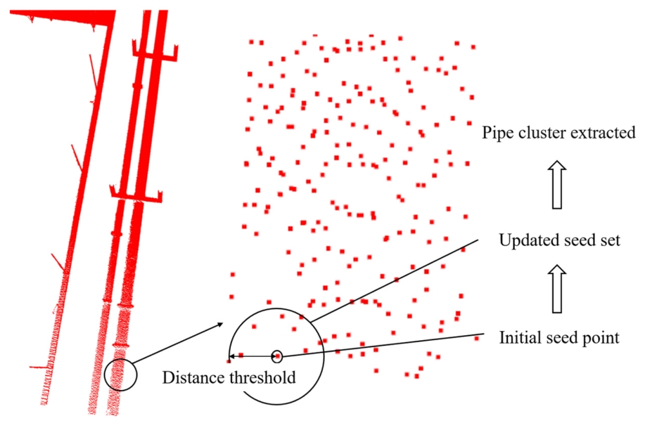
The distance-threshold-based growing procedure uses spatial point distance as the main connectivity feature. To reduce the influence of boundary points, noisy points, and connection regions, candidate seed points are prioritized according to local geometric regularity, with lower-curvature points on relatively smooth pipe surfaces selected first when available. Starting from a seed point, neighboring points within a specified distance threshold are retrieved and added to the current cluster if they satisfy the connectivity condition. The process is repeated until no additional neighboring points can be added. The remaining unprocessed points are then used to start the next cluster.

As shown in Figure 1, the procedure includes the following steps:

• Select an unprocessed point with relatively small local curvature as the initial seed point and determine the distance threshold.
• Add the selected point to the seed set and the current cluster.
• Extract a seed point from the seed set and retrieve its neighboring points according to a spatial search structure and the distance threshold.
• Add the unprocessed neighboring points to the seed set and remove the current seed point from the seed set after expansion.
• When the seed set becomes empty, the growth of the corresponding pipe cluster is completed. The procedure is repeated until all points are processed.

After the growing procedure, each connected cluster is treated as a scanned pipe candidate, and its boundary is determined by the spatial connectivity defined by the distance threshold. After extracting individual pipes from the scanned point clouds, a set $S=\{S_i{\}}_{i=1}^{N_s}$ can be obtained, where each element $S_i$ represents a scanned pipe point cloud. For the BIM model, individual BIM pipe models are exported and sampled to generate a set $B=\{B_j{\}}_{j=1}^{N_b}$, where each element $B_j$ represents a BIM-derived pipe point cloud.

Since the elements in $S$ and $B$ are unordered, it is necessary to establish the correspondence between the scanned pipe point clouds and the BIM-derived pipe point clouds. This correspondence step is performed after Scan-BIM registration, so the distance-based comparison is conducted under a common coordinate system. For each extracted scanned pipe, the BIM-derived pipe with the minimum scan-to-BIM nearest-neighbor RMSE is regarded as its most likely counterpart.

For a scanned pipe point cloud $S_i=\{{\mathit{p}}_k{\}}_{k=1}^{n_i}$ and a BIM-derived pipe point cloud $B_j=\{{\mathit{q}}_l{\}}_{l=1}^{m_j}$, the nearest-neighbor distance from each scanned point ${\mathit{p}}_k$ to $B_j$ is calculated as:

$$d_k^{ij}=\underset{{\mathit{q}}_l\in B_j}{\min }‖{\mathit{p}}_k-{\mathit{q}}_l‖$$

(7)

The RMSE from $S_i$ to $B_j$ is then calculated as:

$${\mathrm{R}\mathrm{M}\mathrm{S}\mathrm{E}}_{ij}=\sqrt{{\displaystyle \frac{1}{n_i}}{\displaystyle \sum _{k=1}^{n_i}}{\left(d_k^{ij}\right)}^2}$$

(8)

The BIM-derived pipe with the smallest ${\mathrm{R}\mathrm{M}\mathrm{S}\mathrm{E}}_{ij}$ is assigned as the counterpart of $S_i$, and the matched BIM-derived pipe is denoted as $B_{M\left(i\right)}$ in the following slice-level analysis. Here, $n_i$ is the number of scanned points in $S_i$. The distance metric is a one-directional nearest-neighbor distance from the scanned pipe to the BIM-derived pipe and does not require strict one-to-one point pairs. After the minimum-RMSE assignment, the mapped pipe pairs are checked before slice-level discrepancy analysis.

2.3. Pipe-Level and Slice-Level Discrepancy Localization

The critical step in analyzing pipe geometric discrepancies is calculating the magnitude and location of discrepancy between the scanned pipe point cloud and the as-designed BIM model. Overall pipe-level discrepancy measures can provide a general indication of pipe deviation, but they cannot directly indicate where the main discrepancy occurs along the pipe. Therefore, a pipe-level and slice-level discrepancy localization strategy is used in this study.

The overall analysis is first conducted on each entire pipe based on the mapped scan-BIM pipe pairs obtained from Section 2.2. Pipes with overall RMSE values larger than an overall screening threshold $r_o$ are further processed using slice-level discrepancy analysis, while pipes with relatively small overall RMSE values are not further segmented in this step. The threshold is used to focus the localization analysis on pipe pairs with clear overall discrepancies.

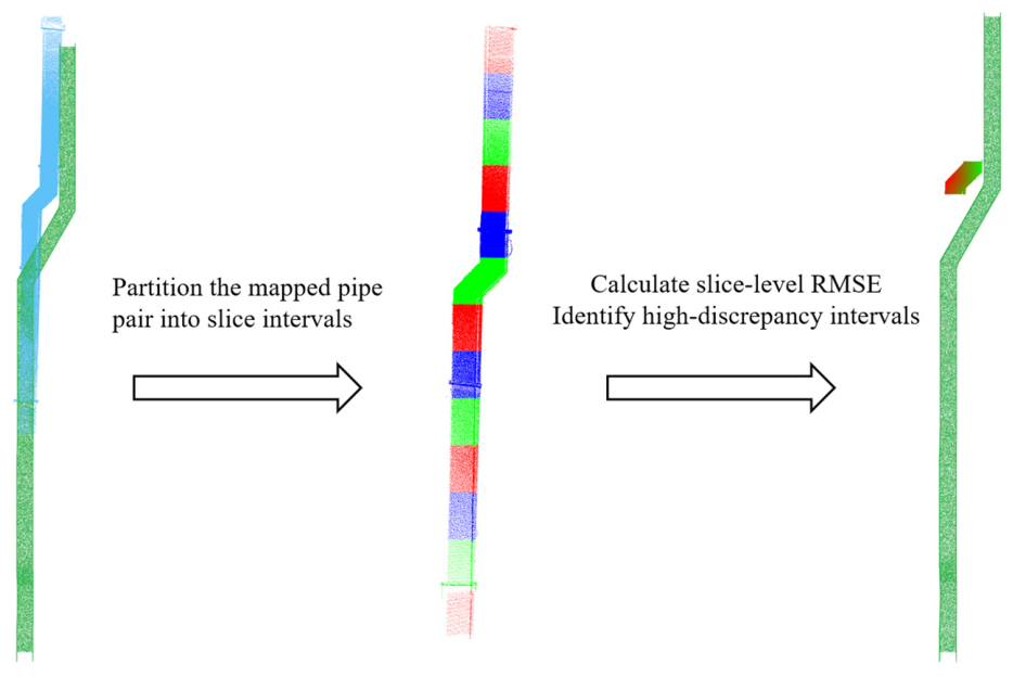
As shown in Figure 2, the pipe-level and slice-level discrepancy localization procedure is as follows:

• Calculate the overall scan-to-BIM RMSE for each mapped pipe pair.
• Select the scanned pipes whose overall RMSE values are larger than the screening threshold.
• Define a one-dimensional relative slicing coordinate along each selected pipe or pipe segment.
• Divide the scanned pipe points into slices according to the relative slicing coordinate.
• Calculate the slice-level scan-to-BIM RMSE values and identify intervals with relatively large discrepancies.
• Output the localized coordinate ranges and RMSE values for visual inspection and engineering interpretation.

To describe the location of a pipe discrepancy along an individual pipe instance, a one-dimensional relative slicing coordinate $s$ is defined. For a straight pipe segment, the coordinate can be obtained by projecting points onto the pipe direction determined from the corresponding BIM-derived pipe segment. Let ${\mathit{c}}_0$ and ${\mathit{c}}_1$ be the two endpoints of the BIM-derived straight pipe segment, and let

$$\mathit{u}={\displaystyle \frac{{\mathit{c}}_1-{\mathit{c}}_0}{‖{\mathit{c}}_1-{\mathit{c}}_0‖}}$$

(9)

be the unit direction vector. For any registered point $\mathit{p}$, its relative slicing coordinate is calculated as:

$$s\left(\mathit{p}\right)=\left(\mathit{p}-{\mathit{c}}_0\right)·\mathit{u}$$

(10)

Both scanned pipe points and BIM-derived pipe points can be described using the same relative slicing coordinate, so the slice partition is defined consistently for the mapped scan-BIM pipe pair. A slice interval is defined as:

$$I_k=\left[s_k-∆s/2, s_k+∆s/2\right]$$

(11)

where $s_k$ is the slice-center coordinate and $∆s$ is the slice length. In the representative classification cases, $s_k$ is reported as a relative coordinate measured from the start of the selected pipe or pipe segment. Equal subdivision is used so that pipes with different lengths can provide the same number of discrete samples for interpolation. The scanned slice is denoted as:

$$S_{i,k}=\left\{\mathit{p}\in S_i | s(\mathit{p})\in I_k\right\}$$

(12)

The slice-level discrepancy at $s_k$ is calculated as the scan-to-BIM RMSE of the scanned slice $S_{i,k}$ with respect to the corresponding BIM-derived pipe point cloud $B_{M\left(i\right)}$:

$$R\left(s_k\right)=\sqrt{{\displaystyle \frac{1}{\left|S_{i,k}\right|}}\sum _{\mathit{p}\in S_{i,k}}{\left(\underset{\mathit{q}\in B_{M\left(i\right)}}{\min }‖\mathit{p}-\mathit{q}‖\right)}^2}$$

(13)

The coordinate $s$ is used to assign points to ordered slice intervals; the point-wise discrepancy within each slice is still calculated by nearest-neighbor distance to the matched BIM-derived pipe. For fittings or elbow regions, $s$ should be interpreted as an ordered local slicing coordinate along the selected pipe path or dominant local direction rather than as a global Cartesian coordinate. This definition keeps the reported slice ranges tied to positions along the selected pipe while avoiding strict dependence on a global coordinate axis.

2.4. Slice-Level Discrepancy Type Classification

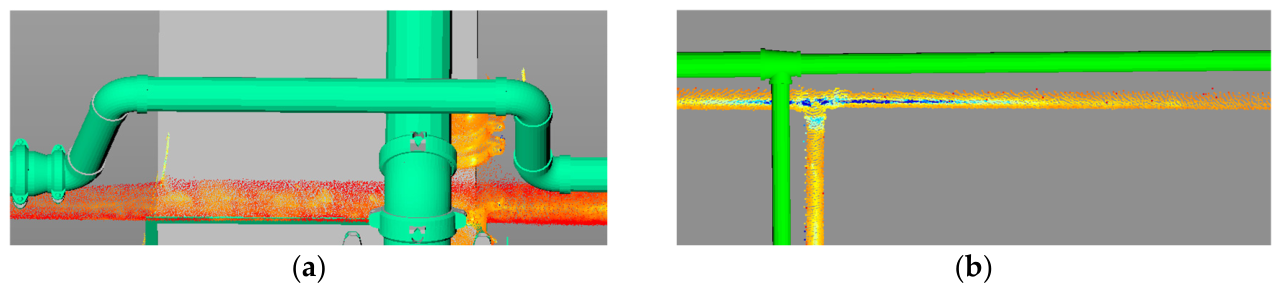
Different pipe discrepancy patterns may correspond to different engineering treatments in construction projects. Discrepancies caused by connection-related local construction practice are denoted as Type 1 pipe discrepancies. These discrepancies are more likely to require on-site checking or local modification. Discrepancies caused by overall pipe deviations or inclinations are denoted as Type 2 pipe discrepancies and may be handled through coordination or design-model adjustment, depending on project requirements. In construction quality control, this distinction helps organize the follow-up checking process: Type 1 results direct attention to local connections, supports, and nearby installation details, whereas Type 2 results direct attention to the overall pipe positioning, installation reference, tolerance requirement, and possible BIM/as-built coordination. This engineering interpretation is consistent with prior studies on MEP coordination and construction rework management, which show that spatial coordination problems, field construction errors, and design or coordination changes can lead to different corrective actions [42,43,44]. Therefore, distinguishing these two types of discrepancies can provide practical support for subsequent engineering decision-making. Representative examples of the two discrepancy patterns are illustrated in Figure 3.

The classification criterion is based on the distribution and variation in slice-level discrepancies along the relative slicing coordinate $s$. The slice-level RMSE values provide a set of discrete discrepancy samples $\left(s_i,R_i\right)$, where $s_i$ is the slice-center coordinate and $R_i$ is the RMSE of the corresponding slice. For the representative classification cases, each selected pipe is divided into the same number of slices so that the resulting $R\left(s\right)$ curves are constructed from comparable discrete samples. Given $m+1$ slice samples with distinct coordinates, polynomial interpolation is used to construct an approximate discrepancy distribution function from these discrete samples:

$$R\left(s\right)=a_0+a_{1}s+\cdots +a_m{s}^m$$

(14)

The coefficients are obtained by constraining the polynomial to pass through the measured slice-level RMSE samples:

$$R\left(s_i\right)=R_i$$

(15)

The derivative used in the classification criterion is then obtained analytically from the interpolation polynomial:

$$R^{\prime }\left(s\right)=a_1+2a_{2}s+\cdots +m{a}_m{s}^{m-1}$$

(16)

The interpolated function $R\left(s\right)$ is used to describe the variation trend of slice-level scan-to-BIM discrepancy along the pipe axis, and $R^{\prime }\left(s\right)$ is used to support the preliminary classification of discrepancy patterns. Because the sign of $R^{\prime }\left(s\right)$ depends on the selected positive direction of the axial coordinate, the derivative magnitude is used to describe the local rate of discrepancy change.

Based on the approximated discrepancy distribution function, a candidate discrepancy interval $I_c$ is first identified using the discrepancy threshold $r_s$:

$$I_c=\left\{s | R(s)\ge r_s\right\}$$

(17)

For a candidate interval $I_c$, the maximum derivative magnitude is defined as:

$$G\left(I_c\right)=\underset{s\in I_c}{\max }\left|R^{\prime }\left(s\right)\right|$$

(18)

The fluctuation amplitude of the derivative within the same candidate interval is defined as:

$$A\left(I_c\right)=\underset{s\in I_c}{\max }{R}^{\prime }\left(s\right)-\underset{s\in I_c}{\min }{R}^{\prime }\left(s\right)$$

(19)

A candidate interval is identified as a Type 1 discrepancy interval when it satisfies the discrepancy threshold, the derivative-magnitude threshold, and the derivative-fluctuation threshold simultaneously:

$$R\left(s\right)\ge r_s, s\in I_c$$

(20)

and

$$G\left(I_c\right)\ge r_s^{\prime }$$

(21)

and

$$A\left(I_c\right)\ge r_f^{\prime }$$

(22)

Here, $r_s$ is the discrepancy threshold of $R\left(s\right)$, $r_s^{\prime }$ is the derivative-magnitude threshold, and $r_f^{\prime }$ is the derivative-fluctuation threshold. Because R(s) is an RMSE-based discrepancy value, $r_s$ is expressed in meters; R’(s) is calculated with respect to the length coordinate s, so $r_s^{\prime }$ and $r_f^{\prime }$ are dimensionless. If the candidate interval does not satisfy the derivative-magnitude and derivative-fluctuation criteria simultaneously, the discrepancy is regarded as more consistent with a Type 2 pattern, such as an overall pipe offset or inclination.

The three thresholds are predefined according to the inspection requirement and are then used consistently for the selected pipe cases. The classification output includes the localized candidate interval and its preliminary Type 1/Type 2 label.

3. Case Study and Results

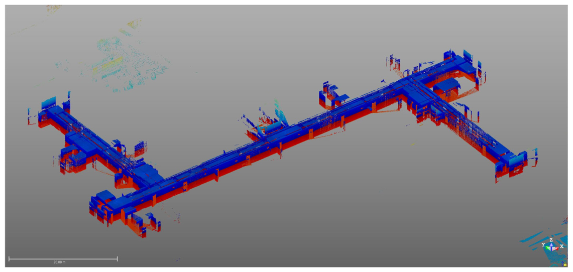
A case study was conducted to examine how the proposed semi-automated Scan-BIM workflow can be applied to MEP pipe discrepancy localization and preliminary type classification in an actual building project. The case project was a student dormitory on the third floor of Zhejiang University International School of Medicine. The point cloud data were collected during construction using a Trimble TX8 terrestrial laser scanner (Trimble Inc., Sunnyvale, CA, USA). The original scanned point clouds are shown in Figure 4.

The case study used two levels of analysis. First, the workflow was applied to a local project region to check pipe clustering and correspondence results, identify pipe instances with relatively large scan-to-BIM discrepancies, and localize maximum-RMSE regions for engineering checking. Second, four representative pipe cases were used to examine the slice-level discrepancy distribution and the preliminary Type 1/Type 2 classification criterion. The first level focuses on project-level screening and coarse local discrepancy localization, while the second level focuses on discrepancy-pattern interpretation using $R\left(s\right)$ and $R^{\prime }\left(s\right)$.

3.1. Case Data and Implementation Settings

The main implementation settings used in the reported case study were as follows. The correspondence distance threshold for ICP-based fine registration was reported as 0.03 m. The growth distance threshold for distance-threshold-based pipe clustering was set to 0.05 m. For project-level local discrepancy localization, the overall RMSE screening threshold was set to 0.08 m, and a fixed 0.4 m physical interval was used along the slicing direction to identify local regions with large RMSE values. This 0.4 m interval was used to obtain practical local ranges for site checking and maximum-RMSE reporting, rather than to construct the discrepancy distribution function.

For the representative discrepancy-function cases, each selected pipe was divided into eight equal slices. The equal-slice strategy was used because applying the same 0.4 m physical interval to pipes with different lengths would lead to inconsistent sample numbers and could provide too few interpolation samples for short pipes. Therefore, the two slicing settings serve different purposes: the 0.4 m interval supports project-level coarse localization, whereas the equal-slice strategy supports comparable $R\left(s\right)$-based interpretation among representative cases.

Open3D (version 0.17.0) was used for point cloud input/output, basic geometric operations, ICP registration, nearest-neighbor and KD-tree search, distance calculation, and visualization. The case workflow was organized through project-specific scripts for benchmark-component handling, pipe point cloud organization, distance-threshold growing, scan-to-BIM pipe assignment, slice partitioning, RMSE aggregation, and discrepancy classification.

3.2. Scan-BIM Processing and Pipe-Level Discrepancy Localization

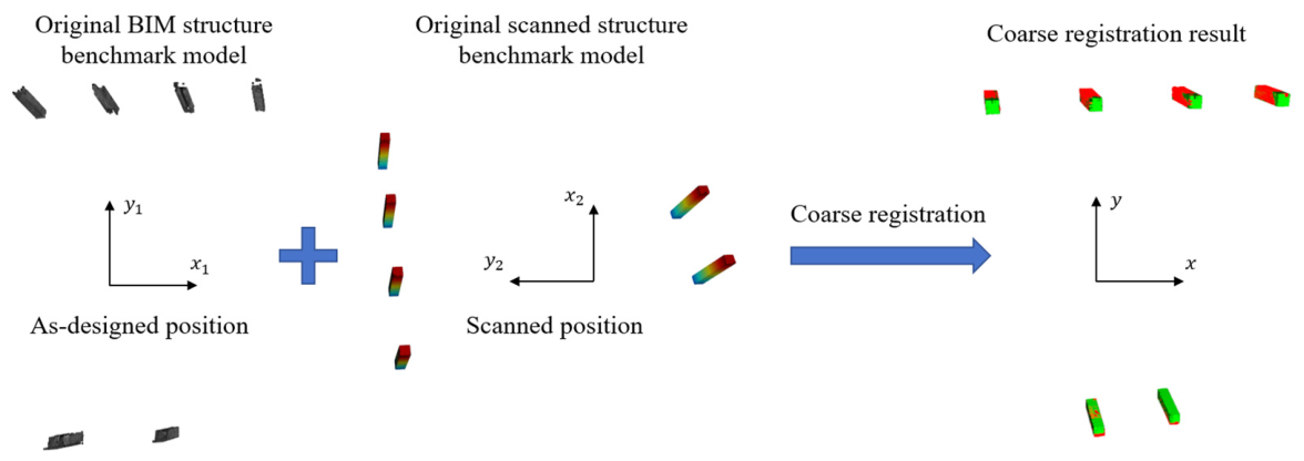
The coarse registration result is shown in Figure 5. In this case, the preprocessing step provided a consistent vertical direction between the scanned point cloud and the BIM model. The coarse registration was then conducted using benchmark structural components. The translation was estimated from the bottom center points of the benchmark bounding boxes, while the horizontal rotation was estimated from the difference between their major-axis directions. This coarse registration result provided an initial alignment for subsequent ICP-based fine registration.

The benchmark structural components were selected or confirmed manually before coarse registration. This was necessary because the scanned scene contained local occlusions and incomplete objects, while stable structural components provide more reliable geometric references than pipe components affected by installation discrepancies. After coarse registration, ICP-based fine registration was used to reduce the residual alignment error between the scanned point cloud and the BIM-derived point cloud.

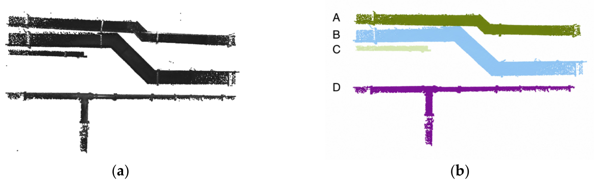
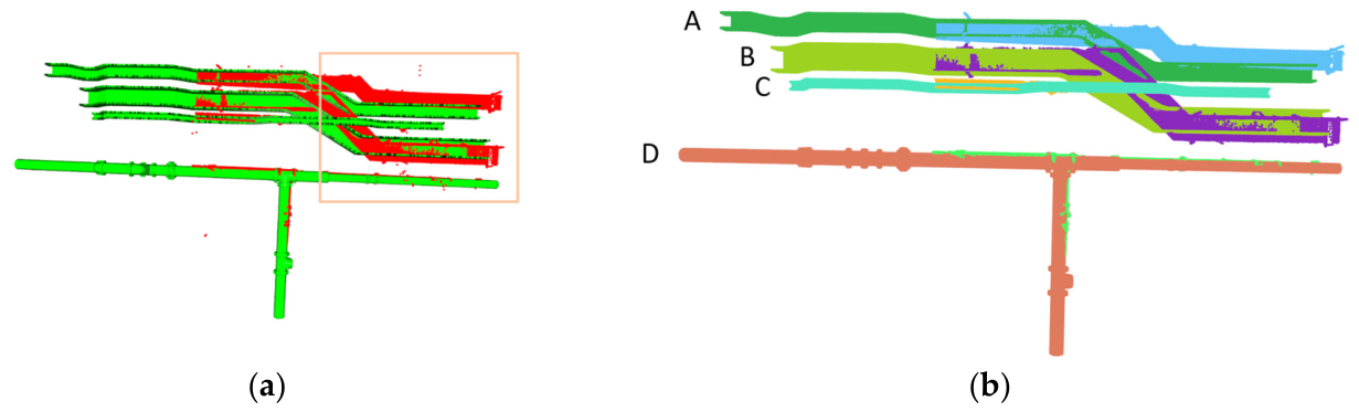
After Scan-BIM registration, the distance-threshold-based growing procedure was used to separate individual pipe instances from the preprocessed pipe point cloud. Figure 6a shows a local region of the preprocessed pipe point cloud in the student dormitory, and Figure 6b shows the corresponding clustering result. Four local project pipes were extracted and denoted as Local Pipes A–D, respectively.

The clustering result was used as the input for pipe correspondence establishment and discrepancy calculation. Because adjacent MEP pipes and fittings are densely arranged in the case region, the extracted clusters were visually checked before the subsequent discrepancy analysis.

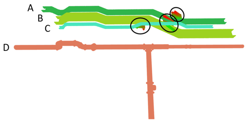
The pipe discrepancy analysis was conducted based on the mapped scan-BIM pipe pairs. For Local Pipes A–D, the Scan-BIM comparison is shown in Figure 7, where relatively large discrepancies can be observed on the right side. The pipe-level and slice-level discrepancy localization procedure described in Section 2.3 was then applied to obtain the localized maximum-RMSE regions, as shown in Figure 8. The corresponding results are summarized in

Table 1. Discrepancy localization results for Local Pipes A–D. The overall RMSE screening threshold was 0.08 m. “—” indicates not applicable because the pipe did not exceed the overall RMSE screening threshold and was not further segmented.

Pipe	Overall RMSE (m)	Screening Result	Max RMSE (m)	Max Discrepancy Region (m)
A	0.17037	Exceeds threshold	0.24908	(−1.61400, −1.21400)
B	0.11047	Exceeds threshold	0.18381	(−2.01760, −1.61760)
C	0.15449	Exceeds threshold	0.17925	(−3.21840, −2.31340)
D	0.02376	Below threshold	—	—

.

For Local Pipes A, B, and C, the overall RMSE values exceeded the screening threshold of 0.08 m, so further slice-level localization was conducted. The localized maximum-RMSE regions provide local physical ranges for subsequent engineering checking. Local Pipe D was not further segmented because its overall RMSE was lower than the screening threshold. These results indicate that the workflow can support pipe-level screening, clustering-result checking, and local discrepancy localization within the case-study region.

3.3. Representative Cases for Slice-Level Discrepancy Classification

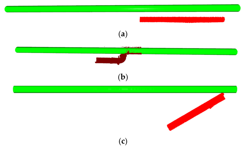
The representative cases used for Type 1/Type 2 classification are denoted as Classification Cases 1–4. Classification Cases 1–3 are shown in Figure 9, including both Type 1 and Type 2 discrepancy patterns. Classification Case 1, shown in Figure 9a, represents the case where the whole pipe is approximately parallel to the corresponding pipe in the as-designed BIM model. Classification Case 2, shown in Figure 9b, represents a discrepancy caused by inconsistent pipe connection practice. Classification Case 3, shown in Figure 9c, represents an overall pipe inclination case.

For the representative discrepancy-function analysis, Classification Cases 1–3 were divided into eight equal slices along the relative slicing coordinate. This equal-slice strategy was used to generate the same number of discrete $\left(s_i,R_i\right)$ samples for each representative case, so that the interpolated discrepancy distribution functions could be compared under a consistent sample structure. The segmentation results are shown in Figure 10. The slice center relative coordinates in

Table 2. Slice center relative coordinates and RMSE values for Classification Cases 1–3.

Case	Overall RMSE (m)	Slice Center Relative Coordinates (m)	Slice RMSE (m)
1	0.25408	[0.127, 0.380, 0.633, 0.886, 1.139, 1.393, 1.646, 1.899]	[0.25006, 0.25618, 0.25787, 0.25699, 0.25542, 0.24854, 0.24517, 0.24240]
2	0.17738	[0.080, 0.241, 0.401, 0.562, 0.722, 0.883, 1.043, 1.204]	[0.24134, 0.24082, 0.24149, 0.24279, 0.20098, 0.08035, 0.00485, 0.00581]
3	0.44966	[0.103, 0.310, 0.517, 0.724, 0.930, 1.137, 1.344, 1.551]	[0.94938, 0.84105, 0.72406, 0.60609, 0.48931, 0.37362, 0.26220, 0.17159]

denote the relative slicing-coordinate position from the start of the selected pipe or pipe segment to the center of each slice.

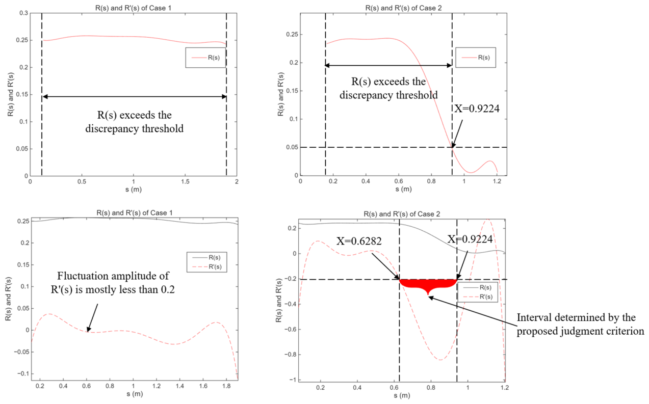
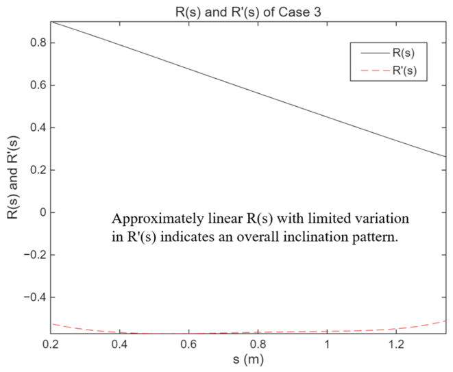
After obtaining the slice-level discrepancy values of each classification case, interpolation was used to approximate the pipe discrepancy distribution function $R\left(s\right)$, and $R\left(s\right)$ was then differentiated to obtain its derivative function $R^{\prime }\left(s\right)$. The functions $R\left(s\right)$ and $R^{\prime }\left(s\right)$ for Classification Cases 1 and 2 are shown in Figure 11, while those for Classification Case 3 are shown in Figure 12.

The preliminary classification criterion used three thresholds in this case study: the discrepancy threshold $r_s=0.05 \mathrm{m}$, the derivative-magnitude threshold $r_s^{\prime }=0.10$, and the derivative-fluctuation threshold $r_f^{\prime }=0.20$. These three thresholds were used together to distinguish local connection-related discrepancy intervals from overall pipe offset or inclination.

For Classification Case 1, which represents an overall parallel offset case, the discrepancy distribution function $R\left(s\right)$ was larger than $r_s$, while $R^{\prime }\left(s\right)$ fluctuated around zero and did not satisfy the derivative-magnitude or derivative-fluctuation conditions. Therefore, the discrepancy in Classification Case 1 was identified as Type 2 pipe discrepancy, which is more consistent with an overall pipe deviation.

For Classification Case 2, which represents a connection-related discrepancy case, using only the threshold of $R\left(s\right)$ would identify a broader discrepancy interval along the pipe. After the derivative-magnitude and derivative-fluctuation conditions were introduced, only the interval with a relatively large change in $R\left(s\right)$ was identified as the Type 1 discrepancy interval. In this case, the obtained Type 1 discrepancy interval was approximately from 0.63 m to 0.92 m along the relative slicing coordinate $s$. Compared with the result based only on the discrepancy threshold, the three-threshold criterion excluded the influence of the overall discrepancy in the front part of Classification Case 2 and provided a more localized identification of the connection-related discrepancy interval.

For Classification Case 3, which represents an overall inclination discrepancy case, $R\left(s\right)$ was larger than $r_s$, and the derivative magnitude was also relatively large. However, the curve of $R\left(s\right)$ shows an approximately linear trend, and $R^{\prime }\left(s\right)$ remains close to a constant value within the plotted interval. Therefore, the derivative-fluctuation condition was not satisfied, and Classification Case 3 was identified as Type 2 pipe discrepancy. This case shows why the derivative-fluctuation threshold is needed in addition to the discrepancy threshold and the derivative-magnitude threshold: an overall inclination may have a large derivative magnitude, but it should not be classified as a local connection-related discrepancy when the derivative variation is limited.

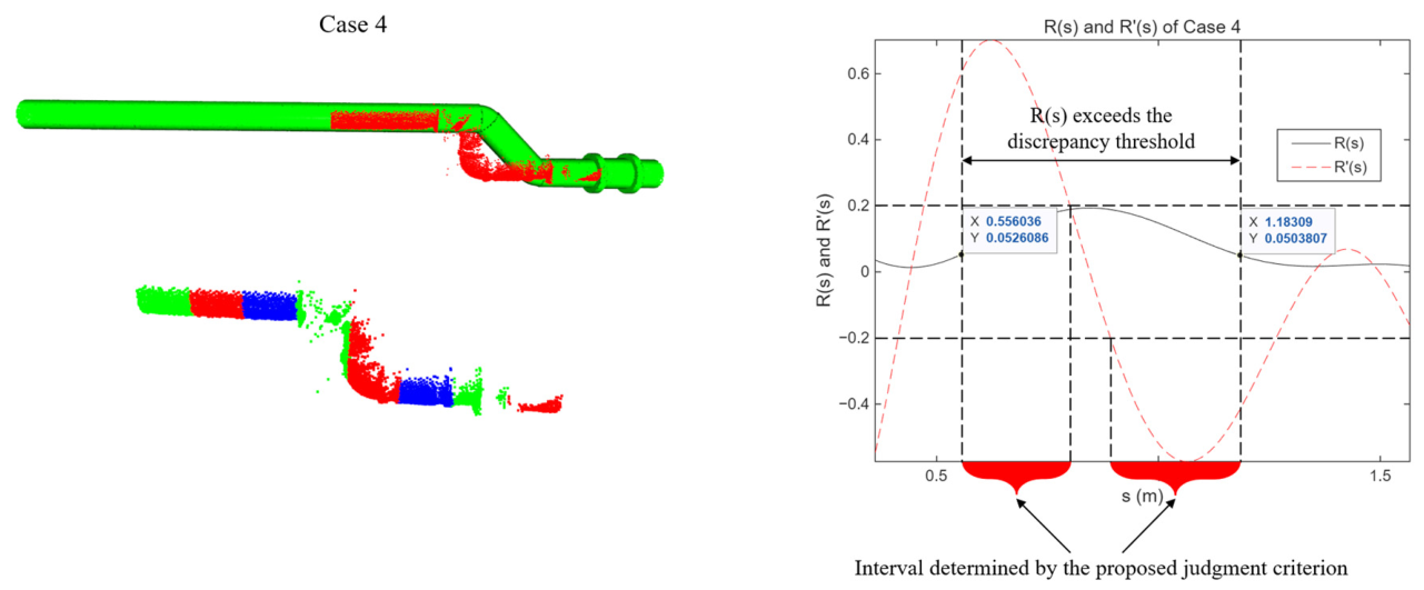
Classification Case 4 was used to further examine the classification criterion. Figure 13 shows the discrepancy case and distribution-function-based analysis of Classification Case 4, and its corresponding slice center relative coordinates and RMSE values are shown in

Table 3. Slice center relative coordinates and RMSE values for Classification Case 4.

Case	Overall RMSE (m)	Slice Center Relative Coordinates (m)	Slice RMSE (m)
4	0.10281	[0.120, 0.361, 0.602, 0.843, 1.084, 1.325, 1.566, 1.807]	[0.02024, 0.03569, 0.08316, 0.19386, 0.10058, 0.01748, 0.01840, 0.01961]

.

Under the classification criterion, the obtained Type 1 discrepancy interval corresponded to the starting and ending positions of the pipe elbow. The result indicates that the proposed slice-level classification can highlight the local transition region associated with the elbow-related construction difference, while the remaining part of Classification Case 4 is closer to the as-designed model.

To examine the local sensitivity of the classification criterion to the three thresholds, a threshold perturbation check was conducted using the reported slice-level values of Classification Cases 1–4. The values compared with the thresholds are summarized in

Table 4. Indicator values used for threshold comparison in the representative classification cases.

Case	${\mathit{R}}_{\mathbf{m}\mathbf{a}\mathbf{x}}$ (m)	$\mathit{G}$	$\mathit{A}$
1	0.25787	0.02709	0.05128
2	0.24279	0.74925	0.75733
3	0.94938	0.56990	0.13217
4	0.19386	0.45934	0.84639

, where $R_{\mathrm{m}\mathrm{a}\mathrm{x}}$ is the maximum discrepancy value, $G$ is the maximum absolute derivative value, and $A$ is the derivative fluctuation amplitude. The baseline threshold group was $\left(r_s,r_s^{\prime },r_f^{\prime })=(0.05 \mathrm{m},0.10,0.20\right)$, and the lower and upper perturbation groups were obtained by changing all three thresholds by −20% and +20%. The classification results under the three threshold groups are shown in

Table 5. Local threshold perturbation check for the representative classification cases. The discrepancy threshold $r_s$ is expressed in meters, whereas the derivative-related thresholds $r_s^{\prime }$ and $r_f^{\prime }$ are dimensionless.

Threshold Group	$\left({\mathit{r}}_{\mathit{s}},{\mathit{r}}_{\mathit{s}}^{\mathbf{\prime }},{\mathit{r}}_{\mathit{f}}^{\mathbf{\prime }}\right)$	Case 1	Case 2	Case 3	Case 4
−20%	(0.040, 0.080, 0.160)	Type 2	Type 1	Type 2	Type 1
Baseline	(0.050, 0.100, 0.200)	Type 2	Type 1	Type 2	Type 1
+20%	(0.060, 0.120, 0.240)	Type 2	Type 1	Type 2	Type 1

.

The Type 1/Type 2 interpretation of the four representative classification cases remained unchanged under the tested threshold perturbations.

Overall, the case study shows that the proposed workflow can check local pipe clustering results, screen pipe instances with relatively large scan-to-BIM discrepancies, localize high-RMSE regions along selected pipes, and provide preliminary Type 1/Type 2 interpretations for representative pipe discrepancy patterns in the reported project.

4. Discussion

The case study results show that the proposed workflow can organize Scan-BIM comparison results into pipe-level screening, local discrepancy localization, and preliminary discrepancy-type interpretation. Existing Scan-BIM studies and construction monitoring studies based on point cloud data have demonstrated the value of registered point clouds for object detection, progress checking, geometric deviation measurement, and as-built model updating [9,10,37,38]. The present workflow extends this comparison from the pipe-object level to the interval level. The pipe-level RMSE indicates whether a pipe differs from the design model, whereas the slice-level result indicates where the main discrepancy is located and whether it is concentrated near a local connection region.

The Type 1/Type 2 classification further supports engineering interpretation of the localized results. A Type 1 result directs attention to local connection regions, fittings, elbows, or local installation practice changes. A Type 2 result directs attention to pipe-level offset, inclination, elevation difference, or broader coordination between the installed pipe and the design model. In this study, the classification is treated as an inspection cue rather than an automatic decision rule for rework, design change, or responsibility attribution. Final decisions still need to be made together with project tolerances, installation constraints, design intent, and stakeholder review.

The workflow builds on mature geometric processing components, including coarse-to-fine registration, distance-threshold-based growing, nearest-neighbor distance calculation, RMSE aggregation, and polynomial interpolation. Combining these components makes the processing route traceable because each output can be related back to pipe correspondence, local distance values, slice aggregation, and the variation of $R\left(s\right)$. Compared with deep learning-based instance segmentation, this geometry-based route requires less labelled training data and keeps the processing logic interpretable, although it still depends on case-specific preprocessing and parameter setting.

From a deployment perspective, the workflow involves field acquisition, software processing, and engineering review costs. For contractors that do not already use laser scanning, the scanner, scanning service, registration software, and trained operators may form the main adoption cost. When TLS data are already collected for construction documentation, progress monitoring, or quality inspection, the additional cost mainly comes from preprocessing, case-specific parameter setting, distance calculation, and engineering interpretation. The algorithmic part uses common point cloud operations and does not require a deep-learning training environment or specialized hardware acceleration for the reported case scale. After registration and preprocessing, pipe-wise correspondence, distance calculation, and slice-level RMSE aggregation can be processed independently for different pipe instances and slice intervals, which provides a basis for future parallel implementation. Therefore, the workflow is more suitable for projects or contractors that already have access to TLS data, and for pipe-dense MEP areas, high-value installation zones, and pre-concealment inspection tasks.

The reported thresholds and intervals are case-study parameters. The clustering radius, ICP correspondence threshold, RMSE screening threshold, slice interval, and Type 1/Type 2 classification thresholds are affected by point density, scanning noise, pipe diameter, expected installation tolerance, and the inspection purpose. The fixed 0.4 m interval used for project-level localization provides a practical physical range for site checking, whereas the eight equal slices used in the representative classification cases provide a consistent number of samples for interpolation. The threshold perturbation check in Section 3 provides local evidence that the Type 1/Type 2 labels of the four representative cases remained unchanged within the tested ±20% perturbation range around the baseline thresholds.

The reliability and interpretation of the workflow are affected by data completeness and by the distance metric used for Scan-BIM comparison. The workflow is most reliable when the target pipe region is sufficiently captured and the scanned pipe instance has a plausible BIM-derived candidate. Occlusions, reflective surfaces, missing scan regions, additional pipes, and severe segmentation errors may affect clustering and correspondence. In addition, the current scan-to-BIM distance is a one-directional nearest-neighbor distance from scanned points to BIM-derived points. This metric is useful for locating scanned points that deviate from the design model, but it is less informative when BIM components are missing from the scan or when the physical source of the increased RMSE is unclear. Therefore, the Type 1/Type 2 interpretation should be read together with the Scan-BIM visualization and engineering context, especially for fittings, elbows, and mixed-defect cases.

5. Conclusions

This study presented a 3D laser scanning and BIM-based workflow for MEP pipe installation discrepancy localization and preliminary discrepancy classification. The workflow integrates Scan-BIM registration, pipe clustering and correspondence, pipe-level RMSE screening, slice-level discrepancy localization, and Type 1/Type 2 interpretation based on the slice-level discrepancy distribution $R\left(s\right)$. Instead of treating a pipe discrepancy only as an overall RMSE value, the workflow summarizes discrepancy variation along selected pipes or pipe segments so that local high-discrepancy intervals can be identified and interpreted.

The case study in a student dormitory project showed that the workflow could separate local pipe instances, screen pipes with relatively large scan-to-BIM discrepancies, and localize maximum-RMSE regions for further field checking. For the representative classification cases, the three-threshold criterion based on the discrepancy value, derivative magnitude, and derivative fluctuation distinguished the reported local connection-related cases from the reported overall offset or inclination cases. The additional threshold check provided supporting evidence for the consistency of these representative classifications within the reported case data.

The main practical value of the workflow is that it connects three levels of information: pipe-level screening, local discrepancy intervals, and preliminary discrepancy-type interpretation. This structure can help engineers narrow the field checking range and relate geometric discrepancy values to possible installation patterns. The workflow is most useful when TLS data and BIM models are already available and when the inspection target contains dense or high-value MEP pipe regions where localized checking is more meaningful than a single overall deviation value.

This study is based on one building project and should be extended before being used as a general performance benchmark. The present validation used case-specific parameters, manual preprocessing and checking, one-directional nearest-neighbor distance calculation, practical field checking, and a limited baseline comparison. Future work will focus on applying the workflow to different building types and MEP layouts, improving pipe centerline and fitting-region processing, evaluating bidirectional or capped distance metrics, conducting more systematic parameter evaluation, and comparing the workflow with representative Scan-BIM baselines under shared data and metrics. These extensions would help assess the robustness of the workflow under different scan densities, pipe diameters, occlusion conditions, and discrepancy patterns.