Optimization of S_a(T₁)-Based Combined Ground Motion Intensity Measure Using Simulated Annealing Algorithm in Seismic Fragility Analysis of RCS Frame Structures

Abstract

This study presents a seismic fragility analysis of reinforced concrete column–steel beam (RCS) frame structures using an enhanced version of the Park–Ang damage model. The applicability of various seismic intensity measures (IMs) in fragility assessment was evaluated. Furthermore, a two-parameter IM was refined through simulated annealing optimization. Initially, the damage evolution of the structure under both near-field and far-field ground motions was investigated using a modified Park–Ang model tailored for RCS systems from the literature. Subsequently, seismic fragility was assessed through multiple stripe analysis, developing fragility curves for distinct damage limit states under the two ground motion types. The effectiveness of 22 different IMs was then examined across these limit states. A two-parameter IM that accounts for the softening period was identified as particularly effective in capturing ground motion uncertainty. This measure was further optimized by applying simulated annealing to minimize the record-to-record variability (β_RTR), targeting its period coefficient (n) and weighting factor (α). Finally, the enhanced IM’s sufficiency and scaling robustness were validated. Results indicate that near-field ground motions induce considerably more severe damage in RCS frames compared to far-field motions, with damage concentrating in lower stories. The optimized IM achieved reductions in β_RTR ranging from 8.7% to 38.1% across different damage states.

1. Introduction

Reinforced concrete column–steel beam (RCS) frame structures effectively integrate the high ductility of steel with the superior load–bearing capacity of concrete. By adopting dry connection techniques, they enable rapid assembly while minimizing environmental impact, aligning well with the development trend of prefabricated construction. These structures demonstrate broad application prospects in modern engineering (Guo et al., 2012 [1]; Ling et al., 2021 [2]; Men et al., 2021 [3]). Therefore, a comprehensive evaluation of their seismic performance is of critical importance.

In Performance–Based Earthquake Engineering (PBEE), the most widely adopted approach is to develop probabilistic evaluation methods or frameworks to achieve accurate assessment and analysis of structural seismic performance, thereby facilitating decision-making by stakeholders (Moehle and Deierlein, 2004 [4]; Stewart et al., 2002 [5]). Two key aspects are involved. First, it is essential to accurately evaluate the seismic damage of RCS frame structures and establish a rational engineering demand model, so as to effectively capture the damage evolution process. Second, select a suitable ground-motion intensity measure (IM) to accurately characterize ground-motion uncertainty. The selection of ground motions depends not only on the structural system under consideration, but also on the engineering demand parameters (Zhang et al., 2025 [6]; Ebrahimian et al., 2015 [7]; Kostinakis et al., 2018 [8]; Du, 2024 [9]; Tidke and Adhikary, 2022 [10]; Pinzón et al., 2020 [11]; Ozmen, 2017 [12]). Consequently, the selection of a damage model, along with the subsequent evaluation of structural damage, exerts a decisive influence on the choice of an appropriate ground-motion intensity measure.

Global structural damage models can generally be classified into response-, deformation- or energy-based models, modal parameter-based models, and stiffness degradation-based models. Among response-based damage models, the use of the conventional maximum inter-story drift ratio as a damage criterion for RCS frame structures may underestimate seismic performance due to inter-story elastic displacements induced by semi-rigid beam–column connections (Song, 2016 [13]; Belleri, 2017 [14]). Among deformation- or energy-based damage models, the structural-level seismic damage model developed from the member-level damage model proposed by Park and Ang (1985 [15]) based on the linear weighted combination of displacement and hysteretic energy (Kunnath et al., 1991 [16]) and its various derivative formulations (Ou et al., 1993 [17]) has gained the most widespread adoption. This study adopts the classical Park–Ang damage model to accurately characterize the damage of RCS structures, thereby providing a reliable basis for subsequent seismic fragility analysis.

Ground motion intensity measures (IMs) are a key component of performance-based earthquake engineering, as they link structural seismic response with seismic hazard. The selection of appropriate and efficient IMs can reduce the dispersion in predicted structural responses, and thus represents a critical step in seismic fragility analysis. Extensive studies have investigated suitable IMs for different types of structures (Riddell, 2007 [18]; Ye et al., 2013 [19]; Zhou and Li, 2015 [20]; Yang et al., 2021 [21]; Zhang et al., 2024 [22]; Lazaridis et al., 2022 [23]; Massumi and Gholami, 2016 [24]). Zhang et al. (2025 [6]) evaluated the seismic fragility of RCS structures under different damage limit states based on near-field and far-field ground motions, using inter-story drift ratio as the damage index, and further optimized the Housner intensity measure through a genetic algorithm. In the present study, when the classical Park–Ang damage model is adopted as the performance assessment parameter, the applicability of different IMs in fragility analysis requires further investigation.

It is noteworthy that the simulated annealing (SA) algorithm, derived from the thermodynamic annealing principle, allows the probabilistic acceptance of inferior solutions based on the Metropolis criterion. This feature endows it with strong global optimization capability, effectively avoiding the tendency of traditional optimization methods to become trapped in local optima. Consequently, it has been widely applied in complex parameter optimization problems in structural engineering (Zhang and Ke, 2009 [25]; Wu et al., 2011 [26]; Weng et al., 2022 [27]). In recent years, this algorithm has also been extensively utilized in earthquake engineering. Shahandashti and Pudasaini (2019 [28]) proposed an SA-based optimization approach combined with a seismic fragility assessment model for pipeline networks, identifying critical pipelines that should be prioritized for retrofit, thereby significantly improving the cost-effectiveness of retrofit strategies. Pudasaini and Shahandashti (2021 [29]) developed an optimization method for seismic retrofit of pipeline systems considering demand criticality and spatial variability of ground motion intensity; by integrating proximity analysis with SA, an economically efficient retrofit strategy was achieved, substantially enhancing post-earthquake water supply reliability. Roy and Shahandashti (2024 [30]) introduced an optimization framework for seismic retrofit of road networks, integrating fragility analysis, traffic simulation, and SA to identify critical combinations of concrete infrastructure for priority strengthening under limited resources, effectively reducing post-earthquake functional disruptions and improving transportation system safety and efficiency. Mase et al. (2024 [31]), through field investigation and back-analysis, determined the bedrock depth and site classification in the downstream area of the Muara Bangkahulu River, revealing high to very high seismic fragility in coastal tourist zones and riverside trade areas, and providing essential data for subsequent seismic risk assessment. In this study, the SA algorithm is employed to optimize ground motion intensity measures, thereby enhancing their applicability in the seismic fragility assessment of RCS structures.

Based on this, the present study focuses on RCS frame structures and employs the classical Park–Ang damage model to accurately characterize structural damage, investigating the evolution of seismic damage under both near-field and far-field ground motions. Furthermore, 22 seismic intensity measures are selected to evaluate their applicability in fragility analysis across different damage limit states. Finally, the SA algorithm is introduced to optimize the parameters of the S_a(T₁)-based combined intensity measure, to minimize the influence of ground motion uncertainty, and the applicability of the optimized measure is verified from the perspectives of sufficiency and scaling robustness.

2. Design Parameters and Numerical Modeling of RCS Frame Structures

2.1. Design Parameters of RCS Frame Structures

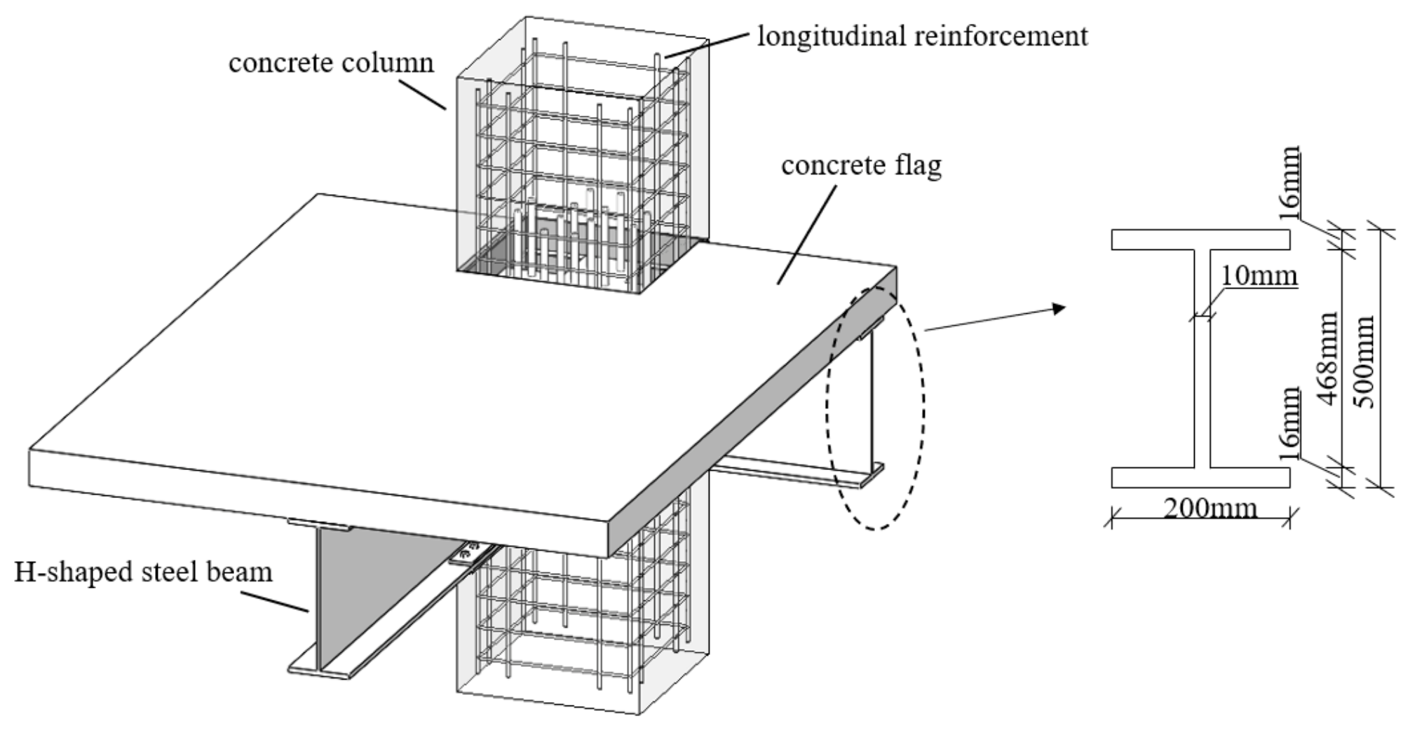
In accordance with the current Chinese design standards (GB/T50010-2010, 2024 [32]; GB/T50011-2010, 2024 [33]; GB 50017-2017, 2017 [34]), a six-story RCS frame structure is selected for analysis, fortified to withstand a seismic precautionary intensity of 8, corresponding to a peak ground acceleration (PGA) of 0.4 g for the rare earthquake. The structure adheres to design seismic Group I and is classified under Site Class II. Detailed design parameters can be found in Zhang et al. (2025 [6]). The building has a bay length of 7 m, with a total length of 35 m, a total building height of 24 m and a standard story height of 4 m. The elevation view of the structure is shown in Figure 1. All columns have a uniform cross-section of 600 × 600 mm² and are constructed using C40 concrete. The longitudinal reinforcement consists of 12 HRB400 steel bars with a diameter of 22 mm. The steel beams are I-shaped sections made of Q235 steel, with dimensions of 500 × 200 × 10 × 16 mm, including a web height of 500 mm, flange width of 200 mm, web thickness of 10 mm, and flange thickness of 16 mm, as illustrated in Figure 2.

As the core load-transfer component of the RCS structure, the beam-through joint configuration is adopted (Sheikh, 1987 [35]; Deierlein, 1988 [36]; Sheikh et al., 1989 [37]; Deierlein et al., 1989 [38]; GB/T50010-2010, 2024 [32]; GB/T50011-2010, 2024 [33]; GB 50017-2017, 2017 [34]), as shown in Figure 2. Beam-to-beam connections use bolted cover plate connections designed according to the equal-strength principle to ensure reliability (Li and Qin, 2019 [39]), with M22 high-strength friction-type bolts of grade 10.9S. The joint is strengthened through the following measures: extended face bearing plates and steel bands are arranged around the full column perimeter; shear studs are uniformly distributed on the top and bottom flanges of the beam as well as at the beam–slab interface, integrating the joint into a whole. This configuration promotes composite action between steel and concrete and prevents concrete crushing in the joint region (Nishiyama et al., 2004 [40]). The face bearing plates and steel bands are made of Q235 steel, with a thickness of 10 mm and a steel band height of 100 mm. The design incorporates the “strong column–weak beam” concept, with a moment amplification factor of 1.4 applied at the column ends (Nishiyama et al., 2004 [40]; GB/T50011-2010, 2024 [33]), thereby enhancing the seismic ductility of the structure. Other detailed configuration parameters can be found in Zhang et al. (2025 [6]).

2.2. Finite Element Modeling of RCS Frame Structures

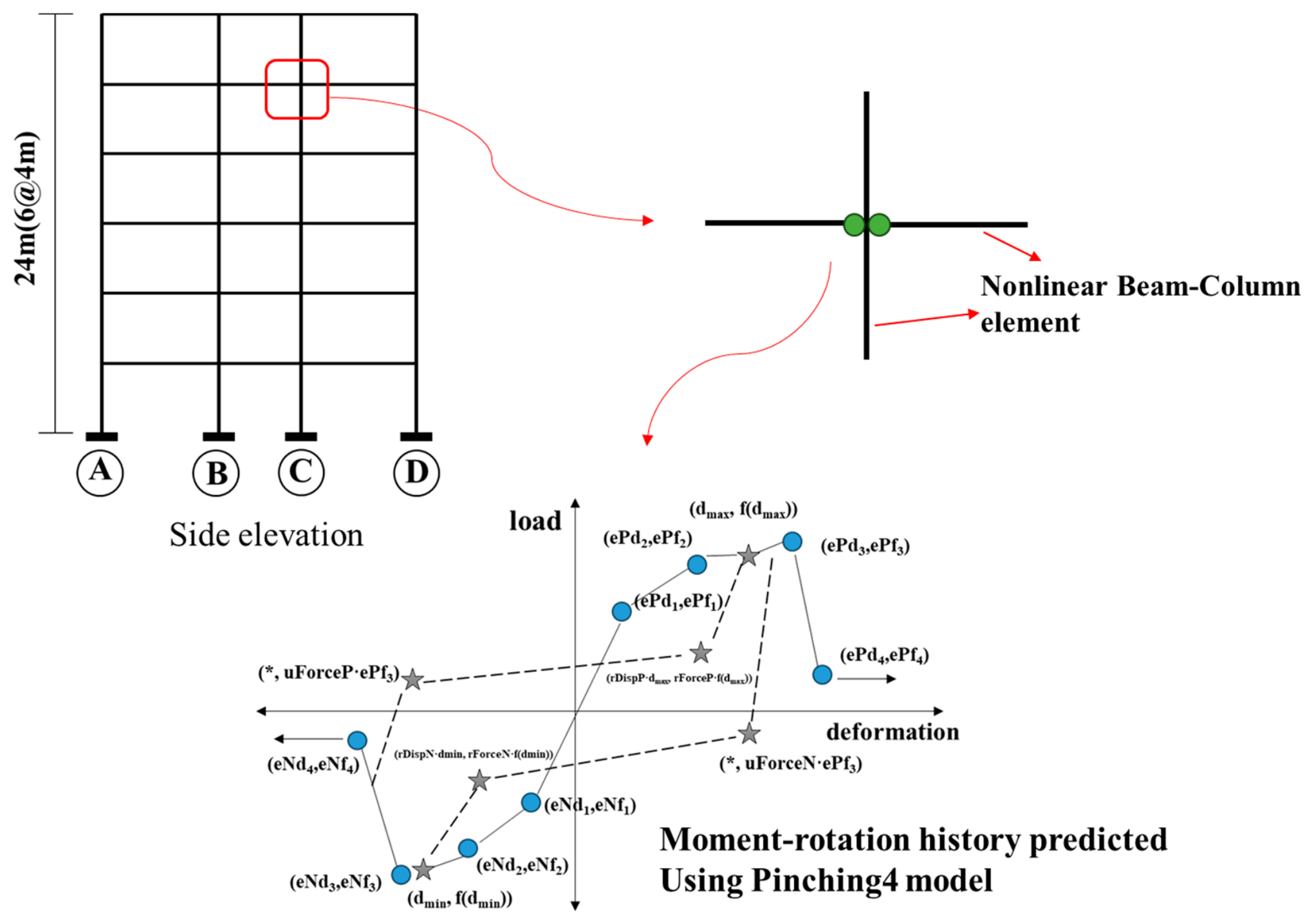
To clearly present the subsequent seismic fragility analysis and the selection of seismic intensity measures, three-dimensional modeling and multi-directional seismic input are not considered in this study (Lucchini et al., 2011 [41]; Kostinakis et al., 2015 [42]). A two-dimensional planar frame model is adopted, and the six-story RCS frame is developed on the OpenSees open-source platform. Structural columns and beams are modeled using nonlinear beam–column elements in OpenSees, as shown in Figure 1. Figure 1 provides an overview of the structural system and numerical modeling strategy. It presents the side elevation of the six-story RCS frame and illustrates the finite element modeling approach. Figure 1 shows that beam–column joints are modeled using zero-length elements with the Pinching4 material model. The inset in Figure 1 displays the hysteretic constitutive relationship of the Pinching4 model, where blue points define the positive and negative envelope curves and dashed lines represent the unloading and reloading paths.

The nonlinear beam–column elements are modeled using distributed plasticity with five Gauss integration points along the element to capture the inelastic behavior. For damage assessment, only the integration points nearest to the ends of beams and columns are used, as inelastic deformation and energy dissipation are concentrated there. The concrete behavior is represented by the Concrete02 model, while the reinforcement and structural steel are modeled using the Steel02 model. The concrete behavior is represented by the Concrete02 model, a standard uniaxial concrete constitutive model in OpenSees that accounts for compressive nonlinearity, tensile softening and stiffness degradation under cyclic loading (Yassin, 1994 [43]). The reinforcement and structural steel are modeled using the Steel02 model, a widely adopted cyclic steel constitutive model that accurately captures the Bauschinger effect and cyclic hardening behavior (Filippou et al., 1983 [44]). The column adopts confined concrete for the core region and unconfined concrete for the outer cover concrete. The transverse confinement provided by stirrups is reflected by modifying the mechanical parameters of core concrete. A Rayleigh damping ratio of 0.05 is used, and the first five natural vibration periods of the OpenSees model are listed in

Table 1. Vibration periods of OpenSees models.

	T1	T2	T3	T4	T5
Periods (s)	1.22	0.34	0.16	0.09	0.06

.

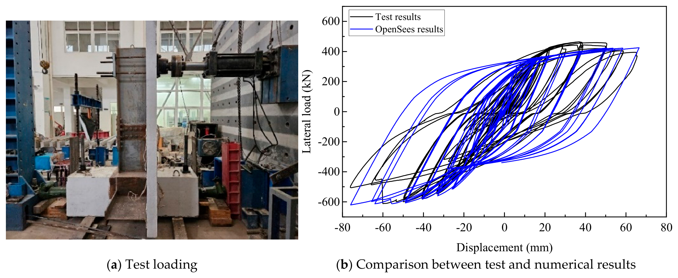
During the modeling process, to accurately simulate the complex nonlinear behavior of beam–column joints, zero-length elements combined with the Pinching4 model from the OpenSees material library are adopted based on experimental data to reproduce the moment–rotation hysteretic behavior. The Pinching4 model is capable of representing pinching effects under cyclic loading, as well as strength and stiffness degradation (Aloisio et al., 2022 [45]; Shahnewaz et al., 2020 [46]). It defines the positive and negative envelope curves through 8 key control points, the values of which are listed in

Table 2. Parameters adopted in the Pinching4 model.

Parameters	Values	Parameters	Values
$ePf1, $ePf2, $ePf3, $ePf4	128.35, 789.31, 1018.98, 827.39	$ePd1, $ePd2, $ePd3, $ePd4	0.00348, 0.01528, 0.0294, 0.03862
$eNf1, $eNf2, $eNf3, $eNf4	−106.08, −612.17.0, −788.8, −671.16	$eNd1, $eNd2, $eNd3, $eNd4	−0.002412, −0.010498, −0.02161, −0.038234
$rDispP, $rDispN	0.3, 0.6	$gK1, $gK2, $gK3, $gK4, $gKLim	0, 0, 0, 0, 0.2
$fFoceP, $fFoceN	0.2, 0.2	$gD1, $gD2, $gD3, $gD4, $gDLim	0.25, 0.25, 0.5, 0.5, 0.5
$uForceP, $uForceN	0.151, 0.15	$gF1, $gF2, $gF3, $gF4, $gFLim	0.0, 0.0, 0.0, 0.0, 0.1
$gE	10.0	$dmgType	energy

and calibrated against low-cycle reversed loading test results of the RCS joint. The parameters used in the Pinching4 model are listed in Table 2. Among these parameters, $ePf_i denotes the force-coordinate coefficient corresponding to the positive envelope curve of the response, while $ePd_i represents the corresponding deformation-coordinate coefficient. Similarly, $eNf_i and $eNd_i denote the force- and deformation-coordinate coefficients associated with the negative envelope curve of the response, respectively. Detailed information on other parameters can be found on the official documentation of the Pinching4 model (Mitra, 2012 [47]). Figure 3 presents a comparison between the numerical results from the OpenSees joint model and the experimental loading results using the parameters in Table 2. The comparison shows that the numerical simulation can effectively reproduce the hysteretic behavior of the top displacement–load relationship observed in the experiments.

3. Selection of Ground Motion Records

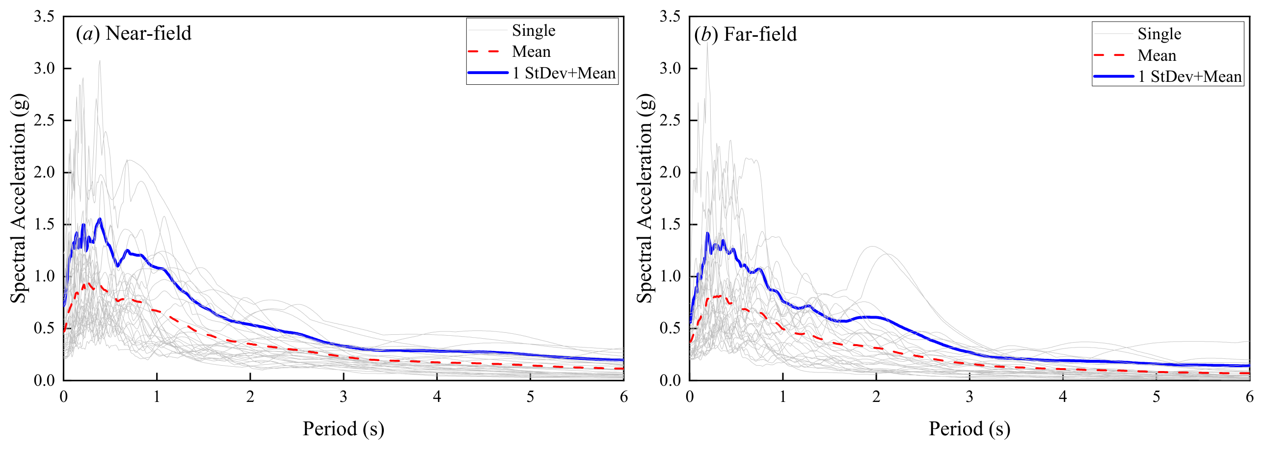
To comprehensively account for the uncertainty in seismic ground motions, two categories of strong motions were considered: pulse-like near-field earthquakes and far-field earthquakes (Zhang et al., 2018 [48]; Zhang and He, 2019 [49]). Each category includes 30 records, as summarized in

Table 3. Selected ground motions (Zhang et al., 2018 [48]; Zhang and He, 2019 [49]).

No.	Near-Field Ground Motions					Far-Field Ground Motions
	Earthquake Event	Component	M	R (km)	PGA (g)	Earthquake Event	Component	M	R (km)	PGA (g)
1	San Fernando	SFERN/PUL164	6.61	1.81	1.22	San Fernando	SFERN/PEL090	6.61	22.77	0.22
2	Imperial Valley-06	IMPVALL.H/H-EMO000	6.53	0.07	0.32	Imperial Valley-06	IMPVALL.H/H-DLT262	6.53	22.03	0.24
3	Imperial Valley-06	IMPVALL.H/H-E04140	6.53	7.05	0.48	Imperial Valley-06	IMPVALL.H/H-E11140	6.53	12.56	0.37
4	Imperial Valley-06	IMPVALL.H/H-E06140	6.53	1.35	0.45	Morgan Hill	MORGAN/G03090	6.19	13.02	0.20
5	Imperial Valley-06	IMPVALL.H/H-E07140	6.53	0.56	0.34	Superstition Hills-02	SUPER.B/B-ICC000	6.54	18.2	0.36
6	Cape Mendocino	CAPEMEND/PET000	7.01	8.18	0.59	Superstition Hills-02	SUPER.B/B-IVW360	6.54	23.85	0.21
7	Northridge-01	NORTHR/RRS228	6.69	6.5	0.87	Loma Prieta	LOMAP/A02043	6.93	43.23	0.27
8	Kobe/Japan	KOBE/KJM000	6.9	0.96	0.83	Loma Prieta	LOMAP/AND250	6.93	20.26	0.25
9	Kocaeli/Turkey	KOCAELI/YPT060	7.51	4.83	0.23	Loma Prieta	LOMAP/OHW000	6.93	74.26	0.29
10	Chi-Chi	CHICHI/TCU052-E	7.62	0.66	0.36	Loma Prieta	LOMAP/SFO000	6.93	58.65	0.24
11	Chi-Chi	CHICHI/TCU065-E	7.62	0.57	0.79	Landers	LANDERS/CLW-LN	7.28	19.74	0.28
12	Chi-Chi	CHICHI/TCU068-E	7.62	0.32	0.51	Landers	LANDERS/YER270	7.28	23.62	0.24
13	Chi-Chi	CHICHI/TCU101-E	7.62	2.11	0.21	Kobe/Japan	KOBE/ABN090	6.9	24.85	0.23
14	Chi-Chi	CHICHI/TCU102-E	7.62	1.49	0.30	Kobe/Japan	KOBE/FKS090	6.9	17.85	0.22
15	Duzce/Turkey	DUZCE/DZC180	7.14	6.58	0.40	Kocaeli/Turkey	KOCAELI/ARE000	7.51	13.49	0.21
16	Loma Prieta	LOMAP/LEX000	6.93	5.02	0.44	Kocaeli/Turkey	KOCAELI/DZC180	7.51	15.37	0.31
17	Bam/Iran	BAM/BAM-L	6.6	1.7	0.81	Chi-Chi	CHICHI/CHY101-E	7.62	9.94	0.34
18	Darfield/New Zealand	DARFIELD/GDLCN55W	7	1.22	0.76	Chi-Chi	CHICHI/TCU045-E	7.62	26	0.47
19	Darfield/New Zealand	DARFIELD/LINCN23E	7	7.11	0.46	Duzce/Turkey	DUZCE/BOL000	7.14	12.04	0.74
20	Darfield/New Zealand	DARFIELD/TPLCN27W	7	6.11	0.30	Hector Mine	HECTOR/HEC000	7.13	11.66	0.27
21	Imperial Valley-06	IMPVALL.H/H-ECC002.AT2	6.53	7.31	0.21	Loma Prieta	LOMAP/WAH000	6.93	17.47	0.37
22	Imperial Valley-06	IMPVALL.H/H-E10050.AT2	6.53	8.6	0.23	Northridge-01	NORTHR/TAR360	6.69	15.6	0.99
23	Imperial Valley-06	IMPVALL.H/H-E05140.AT2	6.53	3.95	0.53	Chi-Chi	CHICHI/TCU088-E	7.62	18.16	0.52
24	Imperial Valley-06	IMPVALL.H/H-EDA270.AT2	6.53	5.09	0.35	Chi-Chi	CHICHI/TCU095-E	7.62	45.18	0.37
25	Imperial Valley-06	IMPVALL.H/H-HVP225.AT2	6.53	7.5	0.26	Niigata/Japan	NIIGATA/NIG023EW	6.63	25.82	0.28
26	Landers	LANDERS/LCN260.AT2	7.28	2.19	0.73	Chuetsu-oki/Japan	CHUETSU/65005EW	6.8	22.74	0.56
27	Chi-Chi	CHICHI/CHY024-E.AT2	7.62	9.62	0.28	Chuetsu-oki/Japan	CHUETSU/65025EW	6.8	11.09	0.65
28	Chi-Chi	CHICHI/TCU049-E.AT2	7.62	3.76	0.28	Chuetsu-oki/Japan	CHUETSU/65056EW	6.8	20.03	0.36
29	Chi-Chi	CHICHI/TCU075-E.AT2	7.62	0.89	0.33	Chuetsu-oki/Japan	CHUETSU/65057EW	6.8	20.00	0.63
30	Chi-Chi	CHICHI/TCU082-E.AT2	7.62	5.16	0.23	Chuetsu-oki/Japan	CHUETSU/6CB51EW	6.8	11.48	0.50

. All records were obtained from the Pacific Earthquake Engineering Research Center (PEER) ground motion database (Ancheta et al., 2014 [50]). The selection procedure follows the recommendations of FEMA P695 (2009 [51]), with a hypocentral distance of 10 km adopted as the boundary between near-field and far-field records. In addition, the selection of near-field events accounts for forward directivity effects, as these are more likely to induce severe structural damage than permanent ground displacement or fling-step effects. Pulse-like characteristics in near-field records were identified using a wavelet-based approach (Baker, 2007 [52]). The acceleration response spectra of the selected ground motions at a 5% damping ratio are presented in Figure 4.

4. Seismic Damage Analysis and Fragility Curves

4.1. Two-Parameter Damage Model

Scholars have developed damage models that integrate deformation-based and energy-based indices. Among these, the most widely adopted approach in engineering practice is the Park–Ang damage model, which captures the combined effects of initial damage exceedance and cumulative plastic damage (Park and Ang, 1985 [15]). Its formulation is given as follows:

$$D={\displaystyle \frac{{\delta }_{\mathrm{m}}}{{\delta }_{\mathrm{u}}}}+{\displaystyle \frac{\beta }{F_{\mathrm{y}}{\delta }_{\mathrm{u}}}}{\displaystyle \int d}E$$

(1)

where δ_m denotes the maximum deformation of the component under seismic loading, δ_u represents the ultimate deformation under monotonic loading, F_y is the yield strength of the component, β is a non-negative parameter, and dE refers to the hysteretic energy dissipated by the component during seismic action.

Most existing damage models are established based on tests of conventional reinforced concrete components, making it difficult to accurately capture the mechanical behavior and damage evolution of steel–concrete composite members. Since the inelastic behavior is confined within plastic zones near the ends of a member, a modified version of the model was, therefore, developed, based on moment, rotation, and dissipated hysteretic energy by Kunnath et al. (1991 [16], 1992 [53]).

For the RCS structure, the phenomenon where the deformation and plastic energy dissipation are mainly concentrated in the plastic hinge area at the end of the components is more pronounced. Men et al. (2020 [54]) further applied this model to specifically assess the damage of the RCS frame structure, which can more effectively characterize the process of structural damage. The proposed formulation is expressed as follows:

$$D={\displaystyle \frac{{\theta }_{\mathrm{m}}}{{\theta }_{\mathrm{u}}}}+{\displaystyle \frac{\beta }{M_{\mathrm{y}}{\theta }_{\mathrm{u}}}}{\displaystyle \int d}E$$

(2)

where θ_m denotes the maximum rotation under seismic loading, θ_u represents the ultimate rotation of the component under monotonic loading, and M_y is the yield strength of the component.

The distribution of damage in building structures under seismic loading is closely related to the distribution of energy dissipation. For the RCS frame structures considered in this study, members with larger bending moments and rotations typically exhibit greater hysteretic energy dissipation and are more susceptible to damage. Therefore, incorporating energy-based weighting into damage assessment provides a more accurate representation of damage distribution. Based on component-level damage models, an energy-weighted approach is adopted to evaluate both story-level and global structural damage (Kunnath et al., 1990 [55]). By using the energy proportion of each component as a weighting factor, the story damage index of the structure can be expressed as follows:

$$D_L={\displaystyle \sum _{i=1}^n{\lambda }_{Mi}}{D}_i$$

(3)

where D_L denotes the seismic damage index of a structural story, D_i represents the seismic damage index of component i, and λ_Mi is the weighting coefficient of component i. The weighting coefficient λ_Mi is defined as the energy proportion of each component (Kunnath et al., 1990 [55]):

$${\lambda }_{Mi}={\displaystyle \frac{E_i}{{\displaystyle \sum E_i}}}$$

(4)

where E_i denotes the energy dissipated by component i, and ∑E_i represents the total energy dissipated by all components within the considered story.

The global damage index of the structure can be obtained using the same approach (Kunnath et al., 1990 [55]):

$$D_O={\displaystyle \sum _{i=1}^n{\lambda }_{Li}}{D}_{Li}$$

(5)

where D_O denotes the global seismic damage index of the structure, D_Li represents the seismic damage index of the i-th story, and λ_Li is the weighting coefficient for each story. The weighting coefficient λ_Li is defined as the proportion of energy dissipated by the corresponding story E_Li (Kunnath et al., 1990 [55]):

$${\lambda }_{Li}={\displaystyle \frac{E_{Li}}{{\displaystyle \sum E_{Li}}}}$$

(6)

It should be noted that the energy-weighted approach has specific applicable conditions. Kunnath and Park (1990 [55]) pointed out that components with greater hysteretic energy dissipation contribute more to overall structural damage. Thus, component and story weighting coefficients are defined by their respective energy dissipation ratios. This method is suitable for RCS frames where inelastic behavior is concentrated in member-end plastic hinges. However, it may underestimate brittle failures such as concrete crushing or reinforcement fracture.

4.2. Damage Analysis and Quantitative Indicators for RCS Frame Structures

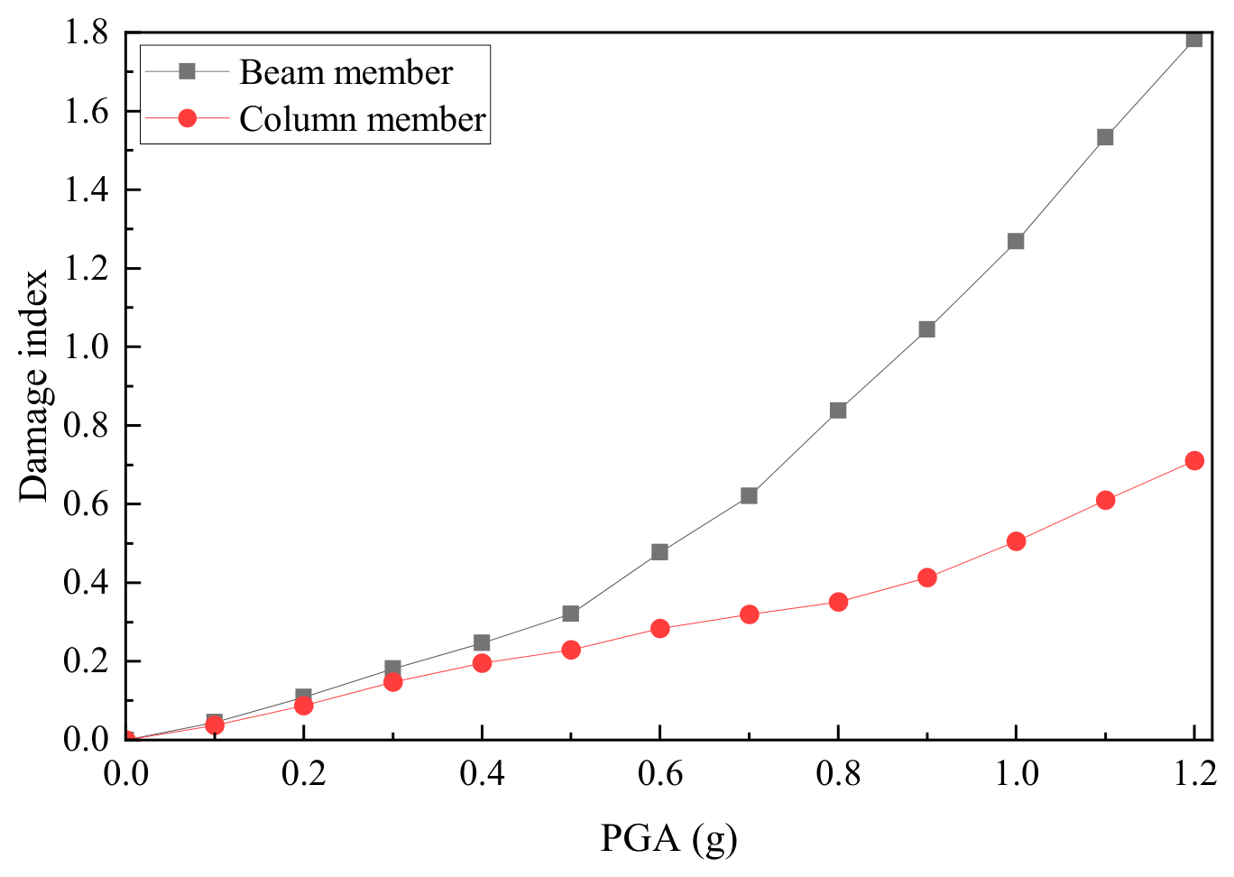
The selected ground motions were amplitude-scaled, with the peak ground acceleration (PGA) of each record increased from 0.1 g to 1.5 g in increments of 0.1 g. Nonlinear time-history analyses were performed on a six-story RCS frame structure using OpenSees, from which member bending moments and rotations were obtained to evaluate component damage. Due to the large number of beams and columns, only representative results are presented. Specifically, the responses of the beam at the second floor between grid A and grid B, and the base column at grid A (as shown in Figure 1), are reported under near-field ground motion No.1 SFERN/PUL164. This record was selected as the representative case because it is a typical pulse-like near-field record conforming to FEMA P695 standards, with a very short epicentral distance of 1.81 km and a significant forward directivity velocity pulse effect. As the record with the highest PGA (1.22 g) among the 30 selected near-field ground motions, it can fully demonstrate the complete damage evolution process of the structure from the elastic stage to the severe damage stage close to collapse. In addition, this record has been widely used in previous seismic studies of RCS frame structures, ensuring good comparability of our results with existing literature. Structural non-convergence occurred when the PGA exceeded 1.2 g. This numerical non-convergence is essentially a computational manifestation of structural failure, triggered by the extensive development of plastic hinges at beam and column ends, which led to severe stiffness and strength degradation. Thus, it indicates that the structure has reached a severe damage state close to collapse; therefore, results corresponding to PGA levels from 0.1 g to 1.2 g are provided in

Table 4. Damage calculation results of the beam at the second floor between grid A and grid B under different ground motions.

PGA	θm (rad)	θu (rad)	My (kN·m)	dE (kNm·rad)	D
0.1 g	0.00087	0.036	737.82	0.6871	0.0453
0.2 g	0.002	0.036	737.82	1.6980	0.1088
0.3 g	0.0028	0.036	737.82	3.3714	0.1815
0.4 g	0.0031	0.036	737.82	5.1953	0.2468
0.5 g	0.0037	0.036	737.82	7.1523	0.3206
0.6 g	0.0039	0.036	737.82	12.039	0.4772
0.7 g	0.0038	0.036	737.82	16.864	0.6204
0.8 g	0.0039	0.036	737.82	23.868	0.8386
0.9 g	0.0041	0.036	737.82	30.441	1.0444
1.0 g	0.0057	0.036	737.82	36.343	1.2685
1.1 g	0.0080	0.036	737.82	42.909	1.5330
1.2 g	0.0105	0.036	737.82	48.819	1.7833

and

Table 5. Damage calculation results of the first-story column at grid A under different ground motions.

PGA	θm (rad)	θu (rad)	My (kN·m)	dE (kNm·rad)	D
0.1 g	0.0016	0.053	791.39	1.0586	0.0376
0.2 g	0.0036	0.053	791.39	2.8528	0.0880
0.3 g	0.0059	0.053	791.39	5.2324	0.1477
0.4 g	0.0082	0.053	791.39	6.1000	0.1962
0.5 g	0.0099	0.053	791.39	6.2027	0.2296
0.6 g	0.0110	0.053	791.39	11.117	0.2838
0.7 g	0.0108	0.053	791.39	16.771	0.3203
0.8 g	0.0103	0.053	791.39	22.291	0.3517
0.9 g	0.0111	0.053	791.39	28.802	0.4129
1.0 g	0.0132	0.053	791.39	36.522	0.5062
1.1 g	0.0155	0.053	791.39	45.132	0.6106
1.2 g	0.0181	0.053	791.39	52.404	0.7107

. Figure 5 illustrates the damage evolution of beams and columns. Structural damage exhibits a pronounced nonlinear increase with increasing seismic intensity. Under identical conditions, damage in steel beams develops significantly faster than in concrete columns, which is consistent with the “strong-column, weak-beam” design principle.

In the story damage analysis, the method described in Equation (3) is adopted. First, the damage indices and hysteretic energy dissipation of beam and column members at each story are obtained under different ground motion intensity levels. Then, the weighting coefficient of each component is determined based on the proportion of its energy dissipation relative to the total energy dissipation of the corresponding story. Finally, the story damage index is calculated by summing the products of the component damage indices and their respective weighting coefficients.

Table 6. Story damage calculation results under near-field ground motion SFERN/PUL164 scaled to 0.4 g.

	Member	Beam 1	Beam 2	Beam 3	Column 1	Column 2	Column 3	Column 4	DL
Floor
1	D	0.25	0.13	0.2	0.20	0.23	0.24	0.18	0.22
	dE (kNm·rad)	8.90	5.36	8.89	12.20	12.97	14.25	8.84
2	D	0.29	0.19	0.29	0.13	0.20	0.20	0.15	0.19
	dE (kNm·rad)	10.80	7.68	10.67	24.35	33.82	34.72	26.38
3	D	0.25	0.17	0.25	0.10	0.16	0.17	0.11	0.16
	dE (kNm·rad)	9.12	6.85	9.00	20.44	30.00	30.90	22.18
4	D	0.21	0.13	0.21	0.12	0.16	0.16	0.13	0.15
	dE (kNm·rad)	7.79	5.05	7.62	17.09	24.31	24.61	18.02
5	D	0.19	0.09	0.17	0.12	0.16	0.16	0.12	0.14
	dE (kNm·rad)	6.72	3.15	6.62	15.72	18.70	19.04	15.83
6	D	0.15	0.07	0.13	0.12	0.14	0.14	0.12	0.13
	dE (kNm·rad)	4.25	1.94	4.28	17.82	15.36	15.16	17.10

and

Table 7. Story damage calculation results under near-field ground motion SFERN/PUL164 scaled to 0.8 g.

	Member	Beam 1	Beam 2	Beam 3	Column 1	Column 2	Column 3	Column 4	DL
Floor
1	D	1.02	0.83	1.15	0.57	0.59	0.77	0.63	0.77
	dE (kNm·rad)	37.20	27.81	41.77	44.98	57.47	71.97	56.18
2	D	0.77	0.66	0.85	0.33	0.42	0.51	0.35	0.49
	dE (kNm·rad)	29.61	24.05	31.79	62.60	74.41	85.62	64.21
3	D	0.60	0.46	0.59	0.27	0.32	0.39	0.27	0.37
	dE (kNm·rad)	23.57	18.49	23.20	50.10	60.16	67.98	47.10
4	D	0.39	0.33	0.40	0.27	0.32	0.35	0.28	0.32
	dE (kNm·rad)	16.83	14.03	17.73	45.64	53.76	55.71	41.51
5	D	0.30	0.26	0.32	0.25	0.35	0.35	0.26	0.30
	dE (kNm·rad)	14.09	9.29	14.33	38.90	49.21	46.50	34.27
6	D	0.23	0.18	0.23	0.21	0.27	0.26	0.24	0.24
	dE (kNm·rad)	8.26	4.84	8.60	30.73	30.45	32.55	34.42

present the damage indices and hysteretic energy dissipation of beam and column members for Stories 1–6 under PGA levels of 0.4 g and 0.8 g, respectively, along with the resulting story damage indices obtained through the aforementioned energy-weighted approach, as shown below.

The evaluation of global structural damage follows the same logic as that of story damage, with story energy dissipation ratios used as weighting factors to compute a weighted average of story damage indices. Specifically, the story damage index D_Li and energy dissipation E_Li at each story are first obtained under different seismic intensity levels. The weighting coefficient λ_Li for each story is then determined based on the proportion of its energy dissipation relative to the total energy dissipation of the structure. The global damage index D_O is subsequently calculated by summing the products of story damage indices and their corresponding weights.

Table 8. Global structural damage under near-field ground motion SFERN/PUL164 scaled to 0.4 g and 0.8 g.

Floor	0.4 g			0.8 g
	DL	ELi (kNm·rad)	Do	DL	ELi (kNm·rad)	Do
1	0.22	71.41	0.17	0.77	337.38	0.46
2	0.19	148.44		0.49	372.29
3	0.16	128.49		0.37	290.60
4	0.15	104.49		0.32	245.21
5	0.14	85.79		0.30	206.60
6	0.13	75.92		0.24	149.83

presents the story damage indices and energy dissipation for Stories 1–6 under near-field ground motion SFERN/PUL164 scaled to 0.4 g and 0.8 g, along with the resulting global structural damage indices obtained through the energy-weighted approach. The results indicate that structural damage is non-uniformly distributed along the height, with lower stories acting as the primary damage concentration zones. Under the 0.8 g seismic excitation, the damage at the base story exceeds that at the top story by more than three times. As the PGA increases from 0.4 g to 0.8 g, the global damage index rises from 0.17 to 0.46, demonstrating a pronounced nonlinear increase in overall structural damage with increasing seismic intensity.

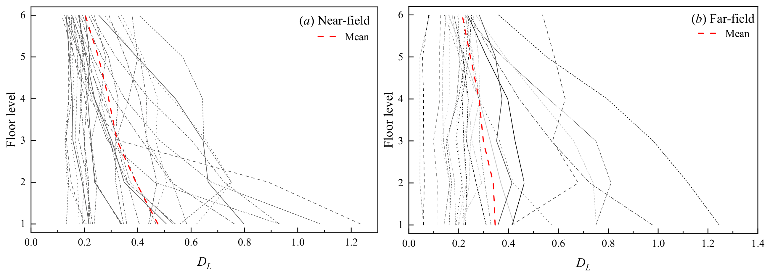
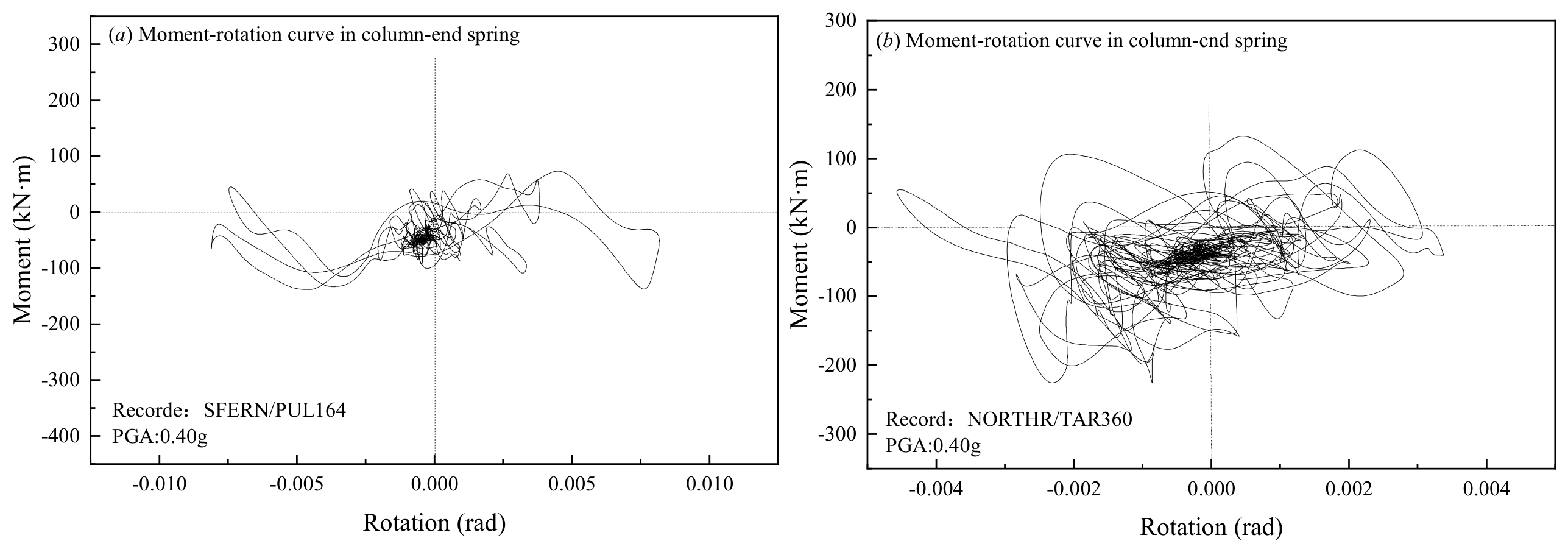
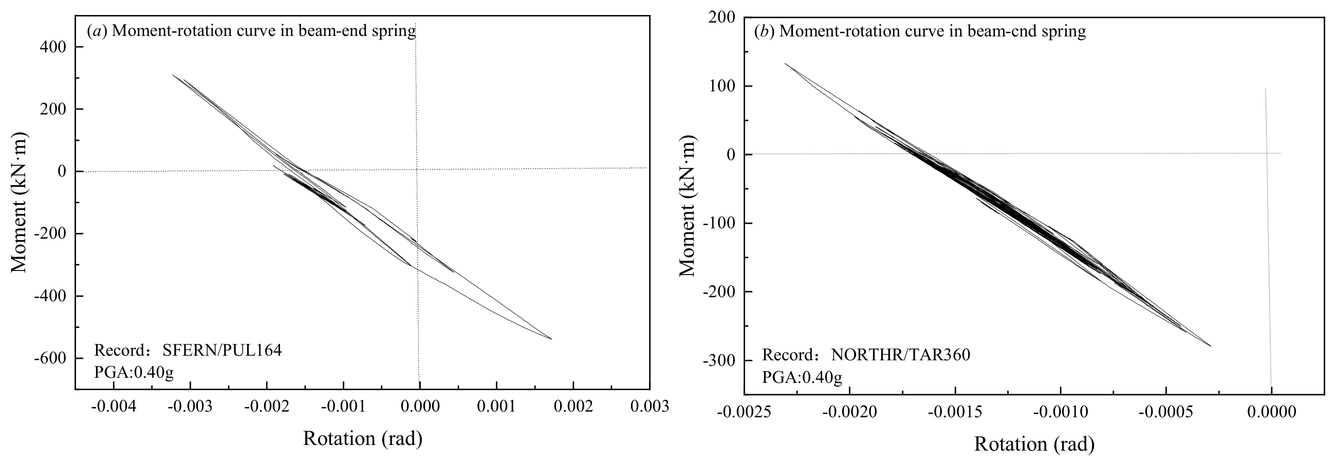
Furthermore, Figure 6 illustrates the distribution of seismic damage along the height of the RCS frame structure under two sets of ground motions scaled to a PGA of 0.4 g. The light gray lines represent the damage distribution of each ground motion record, and the thick red lines represent the average damage distribution of all records in each group. The results indicate that higher levels of damage are concentrated in the lower stories of the building. In terms of average values, seismic damage induced by near-field ground motions is significantly greater than that caused by far-field motions, with peak values exceeding 0.4. Notably, there exists a distinct difference in the vertical damage distribution patterns between the two groups. Both sets of ground motions result in a generally “bottom-heavy” damage distribution, but far-field ground motions show relatively higher damage levels in the upper stories compared to near-field ground motions. This difference can be attributed to the inherent dynamic characteristics of ground motions: near-field ground motions are dominated by short-duration high-amplitude velocity pulses that primarily excite the first mode of the structure, leading to more concentrated damage in the lower stories; whereas far-field ground motions with longer durations and richer long-period components can more effectively excite higher-order modes, resulting in more evenly distributed damage along the height and relatively higher cumulative damage in the upper stories. In addition, Figure 7 and Figure 8 show the moment–rotation hysteretic curves of the column end and beam end of the joint at the top of the first floor slab along axis A, respectively. Figure 7a and Figure 8a correspond to the response under the near-field ground motion No.1 SFERN/PUL164, and Figure 7b and Figure 8b correspond to the response under the far-field ground motion No.22 NORTHR/TAR360. Consistent with the floor distribution characteristics of structural damage, the velocity pulse effect of near-field ground motions makes their response to RCS structures significantly higher than that of far-field ground motions. As shown in Figure 8, the difference is particularly pronounced in the beam end region, where the peak moment exceeds 400 kN·m, and the peak rotation exceeds 0.003 rad in the near field, while the corresponding values in the far field are less than 300 kN·m and 0.0025 rad, respectively.

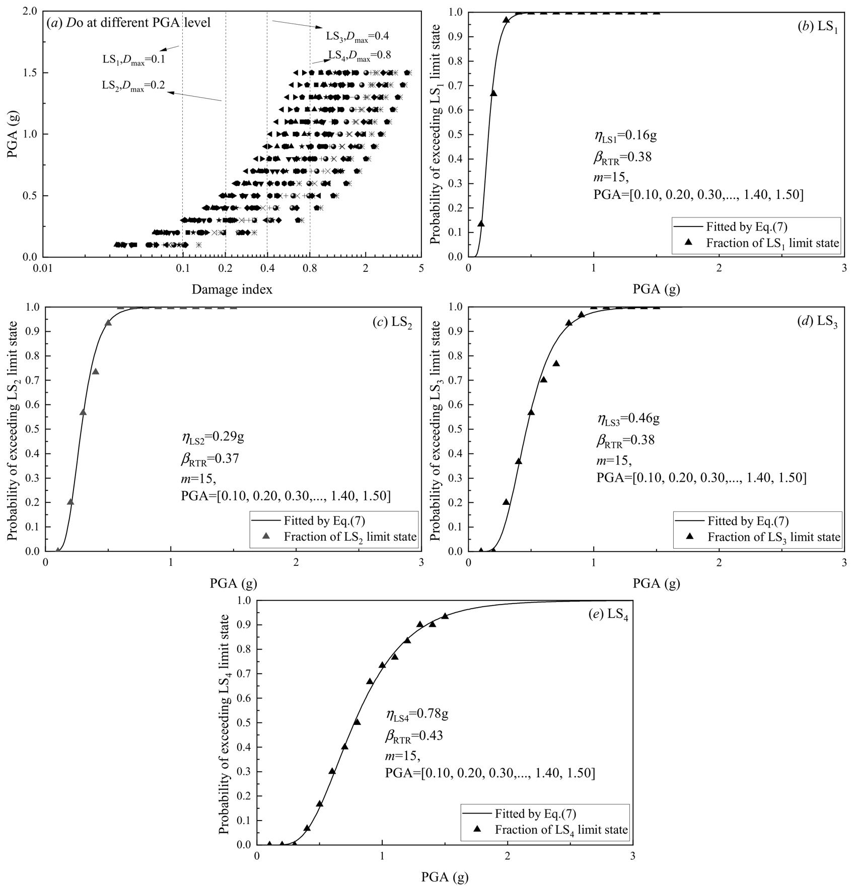
This study adopts the seismic damage classification framework specified in the Code for Seismic Design of Buildings (GB/T50011-2010, 2024 [33]) and, in conjunction with prior studies on damage evolution of RCS frames (Men et al., 2020 [54]; Ma et al., 2018 [56]; Song et al., 2016 [57]), classifies the global damage state of RCS frame structures into five limit states.

Table 9. Damage states of RCS frame structures and corresponding damage index ranges.

Damage State	Minor	Light	Moderate	Severe	Failure
Damage index	0 $\le D_O<$ 0.1	0.1 $\le D_O<$ 0.2	0.2 $\le D_O<$ 0.4	0.4 $\le D_O<$ 0.8	DO $\ge$ 0.8

presents the corresponding ranges of the damage index (D_O). The damage levels are defined as slight damage (denoted as LS₀), minor damage (LS₁), moderate damage (LS₂), severe damage (LS₃), and complete damage (LS₄), with corresponding damage index ranges of 0 $\le D_O<$ 0.1, 0.1 $\le D_O<$ 0.2, 0.2 $\le D_O<$ 0.4, 0.4 $\le D_O<$ 0.8, and D_O $\ge$ 0.8, respectively. This classification provides a quantitative basis for assessing the seismic damage states of RCS frame structures. In addition, it should be noted that the global damage index ranges presented above have certain limitations. For frame structures with non-uniform stiffness or strength distribution along the height, severe localized damage such as soft-story failure may occur, which can lead to global structural collapse even when the global damage index value remains relatively low. In this study, the six-story RCS frame structure was designed strictly in accordance with the latest Chinese seismic design codes, which enforce uniform stiffness and strength distribution to prevent the formation of soft stories. As a result, the structural damage developed gradually and was distributed relatively evenly among the stories in all nonlinear dynamic analyses. For irregular structures or structures with potential soft-story mechanisms, it is recommended to use local story damage indices in conjunction with the global damage index for a comprehensive and accurate seismic performance assessment.

4.3. Multiple Stripe Analysis Method and Fragility Curves

Compared with incremental dynamic analysis (IDA), the multiple-stripe analysis method does not require consideration of all possible ground motion intensity levels that may lead to a given damage limit state. Instead, it evaluates the probability of reaching specified limit states at selected intensity levels; therefore, the multiple stripe analysis method is adopted in this study. Since this approach provides only the proportion of structural responses exceeding a given limit state at discrete intensity levels, the maximum likelihood estimation method is employed to estimate the fragility parameters. Based on the analysis data, it enables the determination of the probability that the structure exceeds a specified limit state. In the framework of maximum likelihood estimation (Baker, 2015 [58]), seismic responses induced by individual ground motions are assumed to be independent. The parameters of the fragility function corresponding to a given limit state can then be obtained from Equation (7):

$$\left\{\widehat{\eta },{\widehat{\beta }}_{\mathrm{RTR}}\right\}=\underset{\eta ,{\beta }_{\mathrm{RTR}}}{\mathrm{argmax}}{\displaystyle \sum _{\mathrm{j}=1}^{\mathrm{m}}\left\{\ln \left(\frac{n_j}{z_j}\right)+z_j\ln \mathsf{\Phi }\left(\frac{\ln \left(I{M}_j/\eta \right)}{{\beta }_{\mathrm{RTR}}}\right)\right.}+\left.\left(n_j-z_j\right)\ln \left[1-\mathsf{\Phi }\left({\displaystyle \frac{\ln \left(I{M}_j/\eta \right)}{{\beta }_{\mathrm{RTR}}}}\right)\right]\right\}$$

(7)

where η denotes the median intensity corresponding to a given limit state, β_RTR is the logarithmic standard deviation representing record-to-record variability of ground motion uncertainty, m is the number of ground motion intensity levels, Φ( ) is the standard normal cumulative distribution function, and z_j is the number of observations in which the specified limit state is reached among the n_j ground motions at intensity level IM_j.

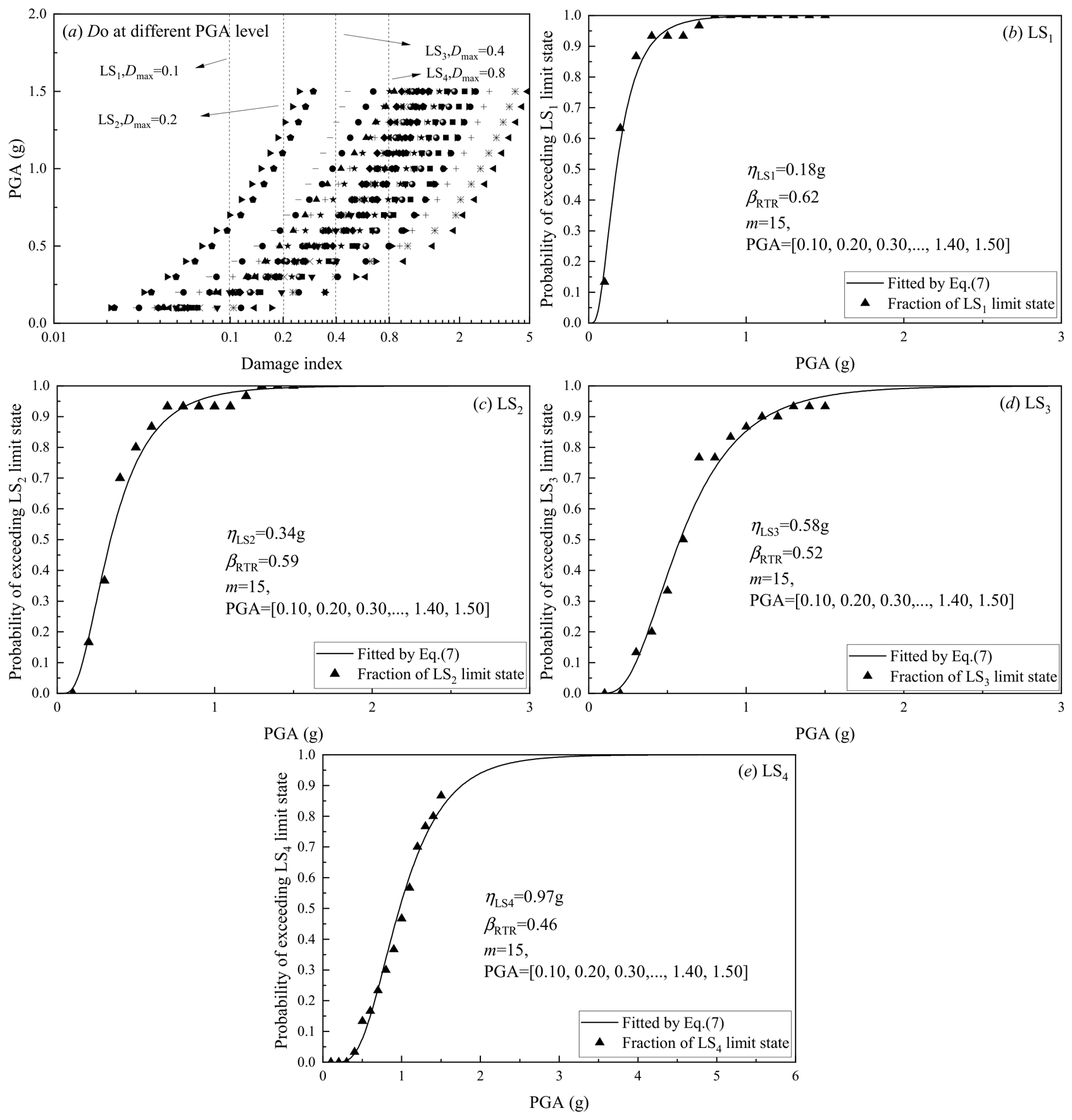
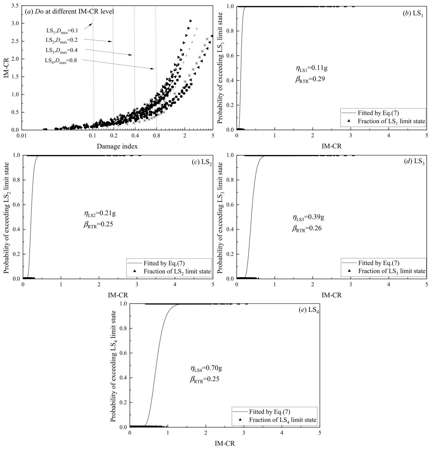
Based on the damage results obtained at 15 ground motion intensity levels with PGA values of 0.10, 0.20, 0.30, 0.40, …, 1.40, and 1.50 g, fragility analyses were conducted for different damage limit states. Figure 9 and Figure 10 present the fragility curves corresponding to four structural damage limit states (LS₁–LS₄) under two types of ground motions. Notably, these curves exhibit distinct trends for different types of seismic records. Under near-field ground motions, the median intensity η for each damage limit state is significantly lower than that under far-field conditions, indicating that the structure is more susceptible to severe damage in near-field earthquakes at the same intensity level. Specifically, the median intensities η for LS₁ to LS₄ are 0.16 g, 0.29 g, 0.46 g, and 0.78 g under near-field motions, and 0.18 g, 0.34 g, 0.58 g, and 0.97 g under far-field motions, respectively. In addition, the logarithmic standard deviation β_RTR under near-field ground motions is generally smaller than that under far-field motions. However, no clear pattern is observed, which can be attributed to the inherent characteristics of both the structural system and the ground motions themselves.

5. Selection and Optimization of Ground Motion Intensity Measures

5.1. Selection of Seismic Intensity Measures

As shown in Table 10, this study investigates 22 seismic intensity measures and summarizes the key parameters involved in each index relevant to RCS structures. The selected intensity measures include amplitude-based indices such as peak ground acceleration (PGA), peak ground velocity (PGV), and peak ground displacement (PGD). In addition, the sustained maximum acceleration (SMA) and sustained maximum velocity (SMV) proposed by Nuttli (1979 [59]) are used to represent the third peak characteristics of the ground motion time history. For spectral-based intensity measures, commonly used indices include spectral acceleration S_a(T₁), spectral velocity S_v(T₁), and spectral displacement S_d(T₁) at the first-mode period. Furthermore, the Housner intensity (HI), which integrates spectral ordinates over a range of structural periods, is also considered. As noted by Zhang et al. (2025 [6]), HI exhibits a strong correlation with seismic structural response. Additional measures include acceleration spectrum intensity (ASI) and velocity spectrum intensity (VSI), originally proposed by Von Thun et al. (1988 [60]). Several intensity measures incorporating period softening effects are also included, such as S*, IM-CR, IM-SR, I_NP, and S_N1. These indices are derived from S_a(T₁) and enhanced by combining multiple spectral components with different exponents to improve their predictive capability.

In addition to softening-period-based measures, intensity indices reflecting higher-mode effects are also considered. The composite measures S*_a12 and S*_a123 proposed by Shome and Cornell (1999 [61]) combine spectral accelerations corresponding to the first two and first three modal periods, respectively. Other higher-mode-sensitive indices include IM₁₂, IM₁₂₃, and S_N2. Finally, S_a,gm(T_i) proposed by Kazantzi and Vamvatsikos (2015 [62]) is also adopted, which simultaneously accounts for both period softening effects and higher-mode contributions.

Table 10. Seismic intensity measures for comparative analysis.

No.	Notation	Definition	Reference
1	PGA	Peak ground acceleration	N.A.
2	PGV	Peak ground velocity	N.A.
3	PGD	Peak ground displacement	N.A.
4	SMA	The third peak in the acceleration	Nuttli, 1979 [59]
5	SMV	The third peak in the velocity time history
6	Sa(T1)	Spectral acceleration at the first vibration period T1	N.A.
7	Sv(T1)	Spectral velocity at the first vibration period T1	N.A.
8	Sd(T1)	Spectral displacement at the first vibration period T1	N.A.
9	HI	$\mathrm{HI}={\displaystyle {\int }_{0.1}^{2.5}P}SV(t)dt$, PSV(t) is the pseudospectral velocity	Housner, 1952 [63]
10	ASI	$\mathrm{ASI}={\displaystyle {\int }_{0.1}^{0.5}{S}_a}(t)dt$	Von Thun et al., 1988 [60]
11	VSI	$\mathrm{VSI}={\displaystyle {\int }_{0.1}^{2.5}{S}_v}(t)dt$
12	S*	S* = (Sa(T1))1−α(Sa(Tf))α Tf is the softened period; α = 0.5, Tf = 2T1	Cordova et al., 2001 [64]
13	IM-CR	$\mathrm{IM}\text{-}\mathrm{CR}=S_a{(T_1)}^{1-\alpha }{S}_a{\left(\sqrt[3]{R_{IM}}\cdot T_1\right)}^{\alpha }$ $R_{IM}$ is the self-adaptive; RIM = 2, α = 0.5	Mehanny, 2009 [65]
14	IM-SR	$\mathrm{IM}\text{-}\mathrm{SR}=S_a{(T_1)}^{1-\alpha }{S}_a{\left(R_{IM}\cdot T_1\right)}^{\alpha }$ $R_{IM}$ is the self-adaptive; RIM = 2, α = 0.5
15	INP	$I_{NP}=S_a(T_1)N_p^a$, $N_p=\sqrt[N]{S_a(T_1)\cdot \dots \cdot S_a(T_N)}/S_a(T_1)$ $T_N$ is the maximum period of interest; α = 0.5, TN = 2T1	Bojórquez and Iervolino, 2011 [66]
16	S*a12	$S_{a12}^{\ast }=0.80S_a(T_1)+0.20S_a(T_2)$	Shome and Cornell, 1999 [61]
17	S*a123	$S_{a123}^{\ast }=0.80S_a(T_1)+0.15S_a(T_2)+0.05S_a(T_3)$
18	IM12	$I{M}_{12}=S_a{({\tau }_a,5\%)}^{1-\beta }{S}_a{({\tau }_b,5\%)}^{\beta }$ ${\tau }_a=T_1, {\tau }_b=T_2, \beta =1/2$	Vamvatsikos and Cornell, 2005 [67]
19	IM123	$I{M}_{123}=S_a{({\tau }_a,5\%)}^{1-\beta -\gamma }{S}_a{({\tau }_b,5\%)}^{\beta }{S}_a{({\tau }_c,5\%)}^{\gamma }$ ${\tau }_a=T_1, {\tau }_b=T_2, {\tau }_c=T_3, \beta =\gamma =1/3$
20	SN1	$S_{N1}=S_a{(T_1)}^{\alpha }\cdot S_a{(C{T}_1)}^{1-\alpha }$ C = 1.5, α = 0.2	Lin et al., 2011 [68]
21	SN2	$S_{N2}=S_a{(T_1)}^{\beta }\cdot S_a{(T_2)}^{1-\beta }$ β = 0.75
22	Sa,gm(Ti)	$S_{a,gm}(T_i)={\left[{\displaystyle \prod _{i=1}^n{S}_a}(T_i)\right]}^{1/n}$ ${(T_i)}_5=\{T_{2m}\min [(T_{2m}+T_{1m})/2,1.5T_{2m}],T_{1m},1.5T_{1m},2T_{1m}\}$	Kazantzi and Vamvatsikos, 2015 [62]

Table 10. Seismic intensity measures for comparative analysis.

No.	Notation	Definition	Reference
1	PGA	Peak ground acceleration	N.A.
2	PGV	Peak ground velocity	N.A.
3	PGD	Peak ground displacement	N.A.
4	SMA	The third peak in the acceleration	Nuttli, 1979 [59]
5	SMV	The third peak in the velocity time history
6	Sa(T1)	Spectral acceleration at the first vibration period T1	N.A.
7	Sv(T1)	Spectral velocity at the first vibration period T1	N.A.
8	Sd(T1)	Spectral displacement at the first vibration period T1	N.A.
9	HI	$\mathrm{HI}={\displaystyle {\int }_{0.1}^{2.5}P}SV(t)dt$, PSV(t) is the pseudospectral velocity	Housner, 1952 [63]
10	ASI	$\mathrm{ASI}={\displaystyle {\int }_{0.1}^{0.5}{S}_a}(t)dt$	Von Thun et al., 1988 [60]
11	VSI	$\mathrm{VSI}={\displaystyle {\int }_{0.1}^{2.5}{S}_v}(t)dt$
12	S*	S* = (Sa(T1))1−α(Sa(Tf))α Tf is the softened period; α = 0.5, Tf = 2T1	Cordova et al., 2001 [64]
13	IM-CR	$\mathrm{IM}\text{-}\mathrm{CR}=S_a{(T_1)}^{1-\alpha }{S}_a{\left(\sqrt[3]{R_{IM}}\cdot T_1\right)}^{\alpha }$ $R_{IM}$ is the self-adaptive; RIM = 2, α = 0.5	Mehanny, 2009 [65]
14	IM-SR	$\mathrm{IM}\text{-}\mathrm{SR}=S_a{(T_1)}^{1-\alpha }{S}_a{\left(R_{IM}\cdot T_1\right)}^{\alpha }$ $R_{IM}$ is the self-adaptive; RIM = 2, α = 0.5
15	INP	$I_{NP}=S_a(T_1)N_p^a$, $N_p=\sqrt[N]{S_a(T_1)\cdot \dots \cdot S_a(T_N)}/S_a(T_1)$ $T_N$ is the maximum period of interest; α = 0.5, TN = 2T1	Bojórquez and Iervolino, 2011 [66]
16	S*a12	$S_{a12}^{\ast }=0.80S_a(T_1)+0.20S_a(T_2)$	Shome and Cornell, 1999 [61]
17	S*a123	$S_{a123}^{\ast }=0.80S_a(T_1)+0.15S_a(T_2)+0.05S_a(T_3)$
18	IM12	$I{M}_{12}=S_a{({\tau }_a,5\%)}^{1-\beta }{S}_a{({\tau }_b,5\%)}^{\beta }$ ${\tau }_a=T_1, {\tau }_b=T_2, \beta =1/2$	Vamvatsikos and Cornell, 2005 [67]
19	IM123	$I{M}_{123}=S_a{({\tau }_a,5\%)}^{1-\beta -\gamma }{S}_a{({\tau }_b,5\%)}^{\beta }{S}_a{({\tau }_c,5\%)}^{\gamma }$ ${\tau }_a=T_1, {\tau }_b=T_2, {\tau }_c=T_3, \beta =\gamma =1/3$
20	SN1	$S_{N1}=S_a{(T_1)}^{\alpha }\cdot S_a{(C{T}_1)}^{1-\alpha }$ C = 1.5, α = 0.2	Lin et al., 2011 [68]
21	SN2	$S_{N2}=S_a{(T_1)}^{\beta }\cdot S_a{(T_2)}^{1-\beta }$ β = 0.75
22	Sa,gm(Ti)	$S_{a,gm}(T_i)={\left[{\displaystyle \prod _{i=1}^n{S}_a}(T_i)\right]}^{1/n}$ ${(T_i)}_5=\{T_{2m}\min [(T_{2m}+T_{1m})/2,1.5T_{2m}],T_{1m},1.5T_{1m},2T_{1m}\}$	Kazantzi and Vamvatsikos, 2015 [62]

5.2. Impact of IMs on β_RTR Estimation

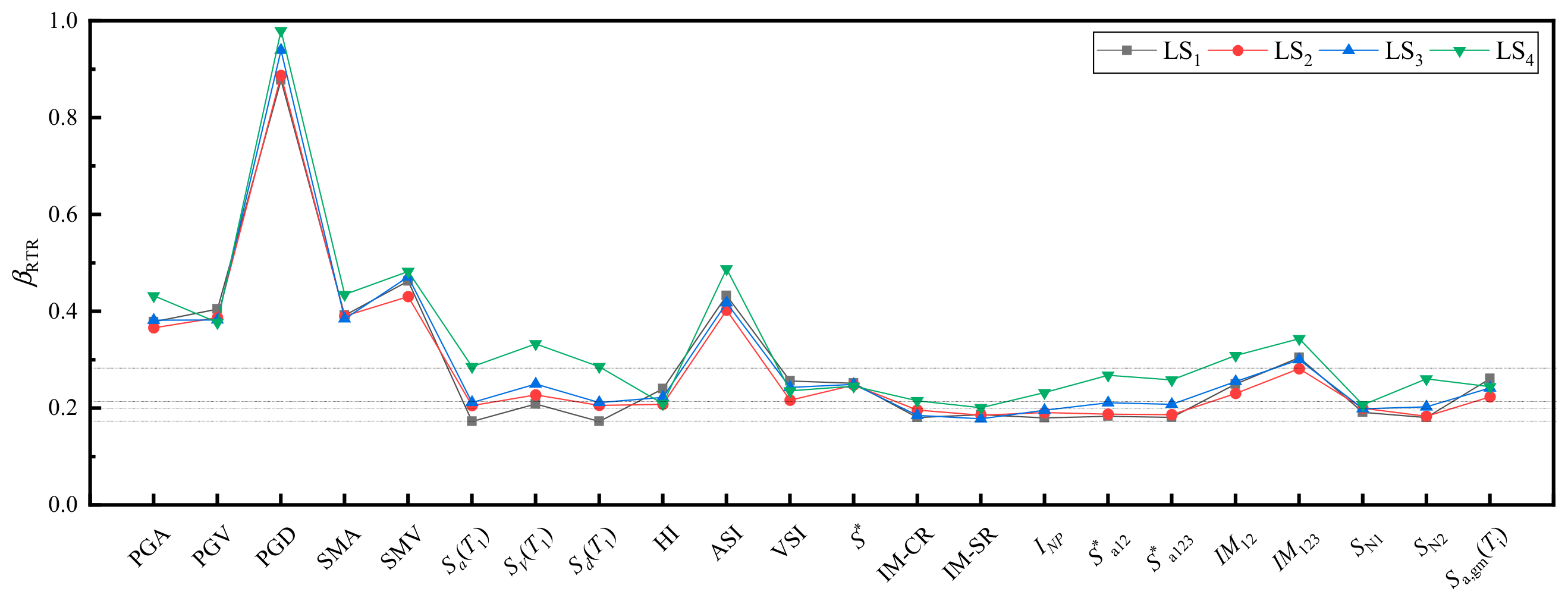
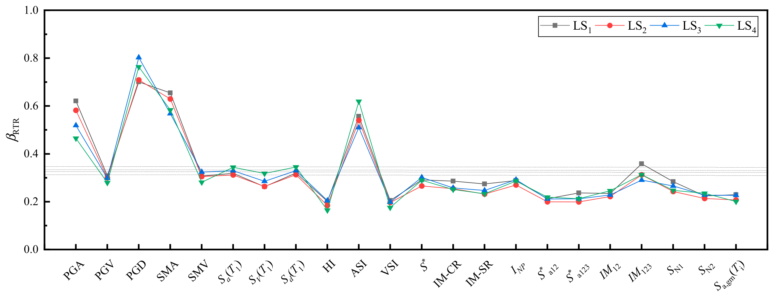
Figure 11 and Figure 12 present the logarithmic standard deviation β_RTR of the 22 selected seismic intensity measures under different damage limit states. It can be clearly observed that, under near-field ground motions, peak-based intensity measures perform worse than spectral-based measures. This is because peak indices only reflect the single-point maximum amplitude of ground motion, failing to capture the spectral characteristics and duration effects that dominate cumulative structural damage. Among the peak-type indices, PGD consistently shows the poorest performance under both types of ground motions, exhibiting lower effectiveness compared to PGA and PGV. This is attributed to the fact that its dominant long-period range deviates significantly from the 1.22 s fundamental period of this 6-story RCS frame. When structural period characteristics are incorporated, S_a(T₁) and S_d(T₁) perform better than their corresponding peak-based counterparts, namely peak ground acceleration (PGA) and peak ground displacement (PGD), as they directly capture the resonance effect between ground motion and the elastic fundamental period of the structure. It is also evident that spectral acceleration-based indices accounting for period softening effects and higher-mode contributions demonstrate superior performance under both near-field and far-field ground motions. In particular, intensity measures considering period softening effects, such as S* and IM-CR, exhibit relatively high stability across different damage limit states, since they match the extended natural period of RCS frames during nonlinear deformation. In addition, the integral-type index, Housner intensity (HI), which is based on pseudo-spectral velocity, also shows favorable performance, consistent with the findings of Zhang et al. (2025 [6]).

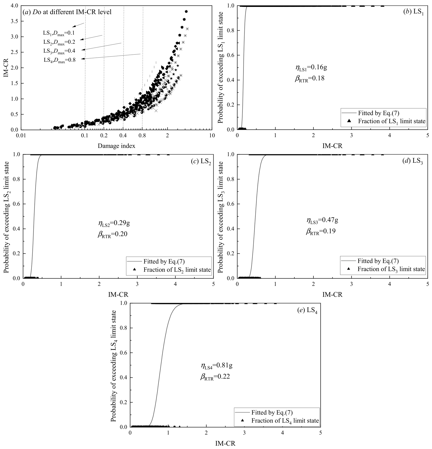
Taking IM-CR as an example, Figure 13 and Figure 14 present the fragility curves for four limit states under near-field and far-field ground motions, respectively. It can be observed that the use of IM-CR leads to relatively low record-to-record variability β_RTR. For both near-field and far-field ground motions, the estimated β_RTR values for each limit state are approximately 0.2 and 0.25, respectively. These fragility curves were derived using the same stripe analysis method and maximum likelihood estimation approach described in detail in Section 4.3, with IM-CR used as the intensity measure instead of PGA.

5.3. Introduction to Optimization Algorithms

In the above analysis, it can be observed that spectral acceleration-based intensity measures incorporating period softening effects perform well under both near-field and far-field ground motions. These measures maintain stable performance across the four damage limit states of the structure and yield relatively small logarithmic standard deviations β_RTR. Such intensity measures are typically constructed as a combination of the spectral acceleration at the first-mode period and the spectral acceleration at an adjusted period. For different damage limit states, there may exist an optimal combination of parameters. Therefore, this study employs the SA algorithm to determine the optimal parameters. By adjusting these parameters, the objective is to minimize the uncertainty of ground motion intensity representation. The optimization problem is formulated as the following constrained minimization problem:

$$\begin{array}{l}\min {\beta }_{\mathrm{RTR}} \\ \mathrm{s}.\mathrm{t}. \left\{\begin{array}{c}{S}_{\mathrm{IMP}}=S_a{(T_1)}^{1-\alpha }{S}_a{(n\cdot T_1)}^{\alpha }\\ 0\le \alpha \le 1\\ 0.1\le n\le 10\end{array}\right.\end{array}$$

(8)

where β_RTR is defined as the objective function, and α and n are the optimization parameters of the intensity measure. Specifically, α represents the weighting factor assigned to the spectral acceleration components, while n denotes the period scaling coefficient. n is used to control the magnitude of the adjusted period. This parameter allows the combined intensity measure to adaptively capture the spectral characteristics of ground motions at different periods relative to the structure’s fundamental elastic period T₁. The range of n from 0.1 to 10 covers all period ranges of engineering interest for seismic response analysis.

The SA algorithm possesses strong global optimization capability and high applicability. By simulating the physical annealing process, it probabilistically accepts temporarily inferior solutions, thereby effectively escaping local optima and converging toward the global optimum. The algorithm imposes few restrictions on the form of the objective function and is characterized by a simple structure and strong robustness. The specific procedure is as follows:

(1)

Initialization: Randomly select (n, α) within the constrained search space and substitute them into the intensity measure to compute the corresponding β_RTR as the initial state. The initial solution is set as the current optimal solution, and the corresponding values of β_RTR, n, and α are stored. The initial temperature is set to T₀ = 100, the minimum temperature is T_min = 0.1, the temperature decay coefficient is α_T = 0.95, and the number of iterations at each temperature level is set to L = 50.

(2)

Fitness function: In the SA algorithm, the quality of a candidate solution is typically evaluated using an energy function or objective function value. A lower energy value indicates that the solution is closer to the global optimum. In this study, the objective is to minimize β_RTR, which is fully consistent with the principle of seeking the minimum-energy state in SA. Therefore, β_RTR is directly adopted as the energy function. During the optimization process, the algorithm probabilistically accepts new solutions with higher energy values, which enables it to escape local optima. As a result, the search process gradually converges toward the global optimal solution corresponding to the minimum energy, the minimum value of the objective function.

$$fit(x)={\displaystyle \frac{1}{{\beta }_{\mathrm{RTR}}(x)}}$$

(9)

where fit(x) denotes the fitness function, and β_RTR(x) represents the objective function value corresponding to the current parameter combination.

(3)

Selection operation: The SA algorithm adopts a probabilistic acceptance strategy for state transitions. Given an initial state S₀, representing the current solution, with energy E₀, a perturbed state S₁ is generated, corresponding to energy E₁. If E₁ < E₀, the new state is accepted and replaces the current state. Otherwise, the new state is accepted with a probability determined by its energy level.

In this study, the objective is to minimize the objective function β_RTR; therefore, the optimal solution can be obtained through the iterative application of this acceptance mechanism. According to statistical thermodynamics, the probabilistic behavior of the annealing process follows the canonical distribution shown in Equation (10) (Rintoul and Torquato., 1997 [69]).

$$P(E_i)={\displaystyle \frac{1}{Z(T)}}{e}^{-{\displaystyle \frac{E_i}{kT}}}$$

(10)

where Z(T) is the normalization constant of the probability distribution, $e^{-{\displaystyle \frac{E_i}{kT}}}$ is the Boltzmann factor, T denotes the current temperature, and k is the Boltzmann constant.

$$Z(T)={\displaystyle \sum _{j=1}^n{e}^{-\frac{E_j}{kT}}}$$

(11)

From Equation (10), it can be inferred that the ratio of probabilities of the system being in the initial state and the new state is equal to the corresponding ratio of the Boltzmann factors.

$$r=e^{-{\displaystyle \frac{E_1-E_0}{kT}}}$$

(12)

Since E₀ $<$ E₁, it follows that r $<$ 1. As described above, the acceptance of a perturbed new state is determined probabilistically. A random number δ uniformly distributed in the interval [0, 1] is generated; if r $>$ δ, the new state S₁ is accepted and replaces the current state S₀; otherwise, the original state is retained. At a fixed temperature, a sequence of new states is generated over a given Markov chain length. If a newly generated state is inferior, Equation (13) is used to determine whether it should replace the current state. As the temperature decreases, the system energy gradually converges toward an equilibrium state. This process constitutes the key Metropolis criterion in the SA algorithm.

Based on the above description, whether the current state S₀ is replaced by the newly generated state S₁ can be determined according to the following Metropolis criterion, which is mathematically expressed as follows:

$$P(S_0\to S_1)=\left\{\begin{array}{ll}1,\hfill & f(S_0)\le f(S_1)\hfill \\ e^{-{\displaystyle \frac{f(S_0)-f(S_1)}{kT}}},\hfill & f(S_0)>f(S_1)\hfill \end{array}\right.$$

(13)

where S denotes the solution space, f(S₀) represents the objective function, and T is the current temperature in the SA algorithm process. f(S₀) and f(S₁) denote the objective function values corresponding to the current state S₀ and the newly generated state S₁, respectively.

(4)

Cooling process: the temperature is updated according to a predefined decay coefficient, thereby progressively reducing the probability of accepting inferior solutions in subsequent iterations and driving the algorithm toward convergence to the optimal solution.

$$T_{k+1}={\alpha }_T\times T_k$$

(14)

Termination criterion: the iteration process repeats steps (3) and (4) while the number of iterations remains below the maximum iteration limit. The algorithm terminates when the temperature decreases to T_min or when the variation of β_RTR over 20 consecutive iterations is less than 0.001. The optimal parameter combination (n, α) is then output, corresponding to the solution with the maximum fitness value and the optimal objective function value.

5.4. Optimization of Intensity Measure Using SA Algorithm

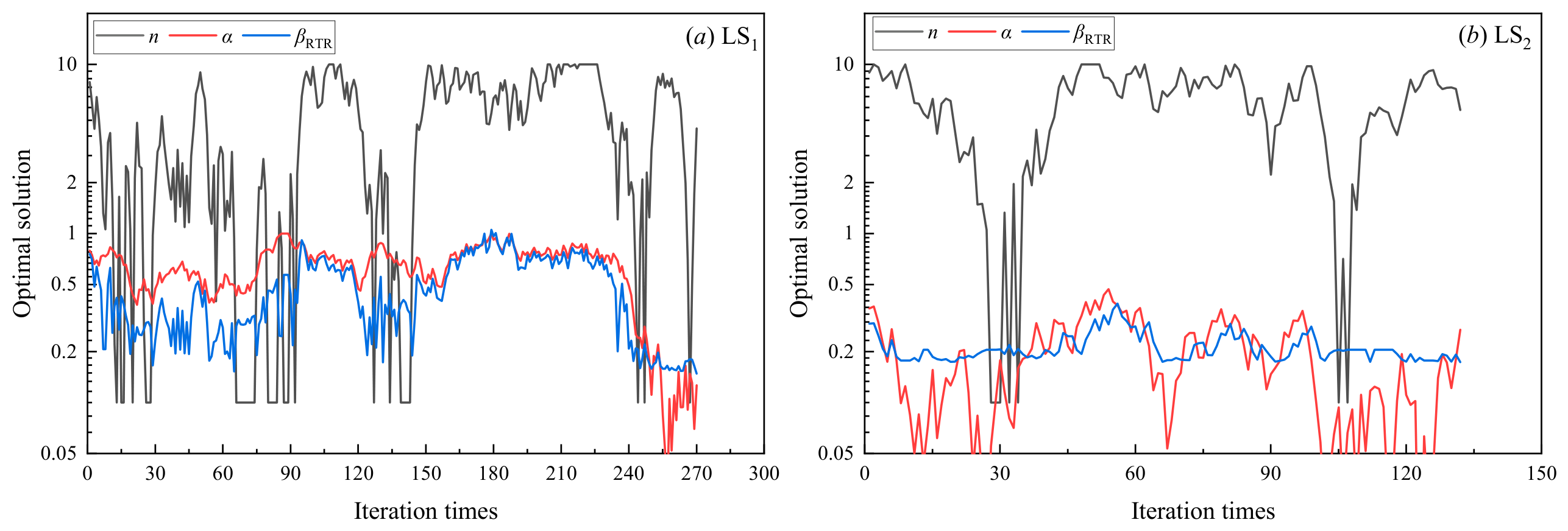
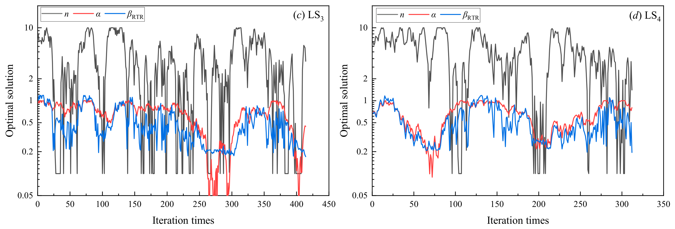
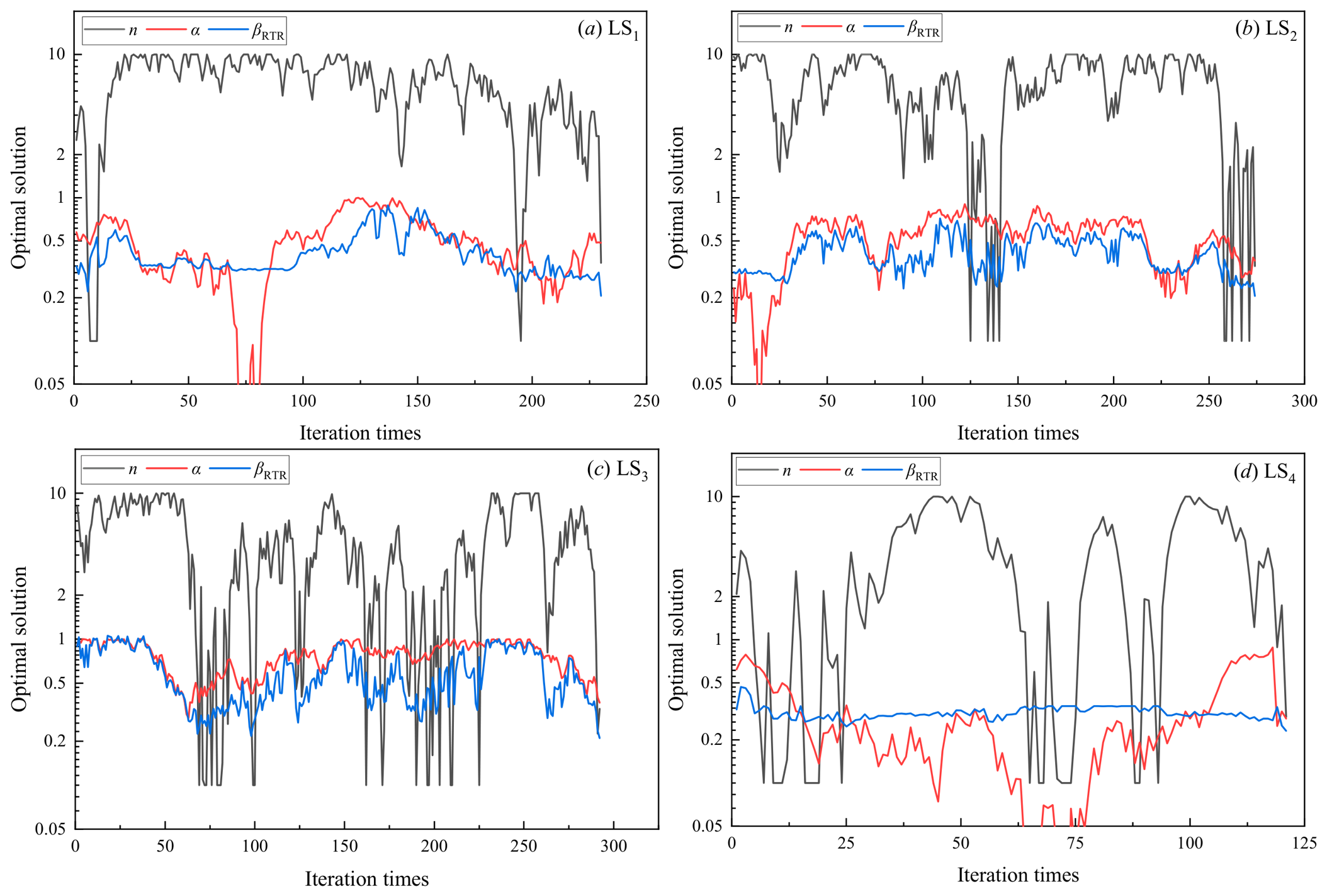
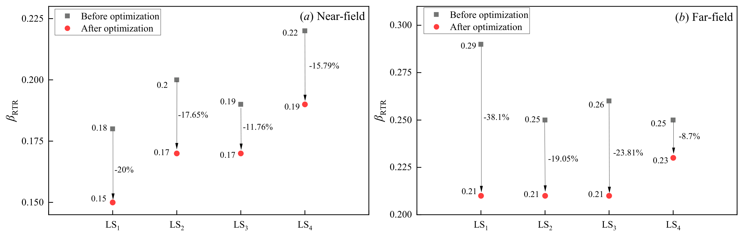
Figure 15 and Figure 16 present the iteration curves of the SA algorithm. After at least 150 iterations, the fitness function converges to the optimal solution, yielding the optimal parameter sets of the proposed ground motion intensity measure under both near-field and far-field conditions, along with the corresponding seismic uncertainty β_RTR for four damage limit states. Under near-field ground motions, the optimal parameter combinations for LS₁, LS₂, LS₃, and LS₄ are (4.19, 0.13), (5.36, 0.27), (3.47, 0.44), and (1.40, 0.81), respectively. Under far-field ground motions, the corresponding parameter sets are (0.35, 0.49), (0.33, 0.36), (0.33, 0.37), and (0.29, 0.28), respectively. As shown in Figure 17, compared with the IM-CR intensity measure, the improved intensity measure S_IMP reduces β_RTR by 20%, 17.65%, 11.76%, and 15.79% for the four damage limit states under near-field conditions, respectively. Under far-field ground motions, the reductions are 38.1%, 19.05%, 23.81%, and 8.7%, respectively. It can be observed that the degree of reduction in β_RTR varies across different damage limit states under both near-field and far-field conditions. Overall, the optimization effect under far-field ground motions is more pronounced than that under near-field conditions.

Table 11. Optimization results of the S_IMP intensity measure via the SA algorithm.

Ground Motions	Limit States	n	α	βRTR	Improvement (%)
Near-field	LS1	4.19	0.13	0.18	20
	LS2	5.36	0.27	0.20	17.65
	LS3	3.47	0.44	0.19	11.76
	LS4	1.4	0.81	0.22	15.79
Far-field	LS1	0.35	0.49	0.29	38.1
	LS2	0.33	0.36	0.25	19.05
	LS3	0.33	0.37	0.26	23.81
	LS4	0.29	0.28	0.25	8.7

further summarizes the optimized parameters of the S_IMP intensity measure. Under near-field ground motions, the period coefficient n for different limit states ranges from 1.4 to 5.36, while the weighting factor α varies between 0.13 and 0.81, indicating relatively wide parameter dispersion. In contrast, under far-field ground motions, n ranges from 0.29 to 0.35 and α ranges from 0.28 to 0.49, showing a much narrower distribution. This suggests that the SA algorithm can adaptively identify more suitable parameter combinations according to different ground motion types. The improved S_IMP intensity measure reduces the seismic uncertainty β_RTR in fragility analysis by approximately 8.7–38.1%. In addition, the degree of reduction in β_RTR varies across different damage limit states under both near-field and far-field conditions. The most significant improvement is observed for the LS₁ state, and overall, the optimization effect under far-field ground motions is more pronounced than that under near-field conditions.

5.5. Sufficiency of the S_IMP Intensity Measure

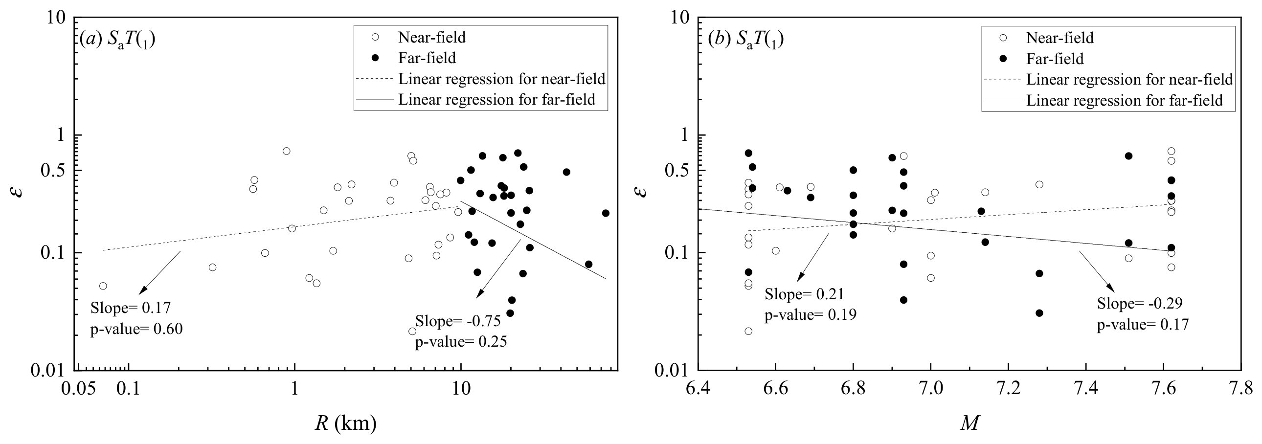
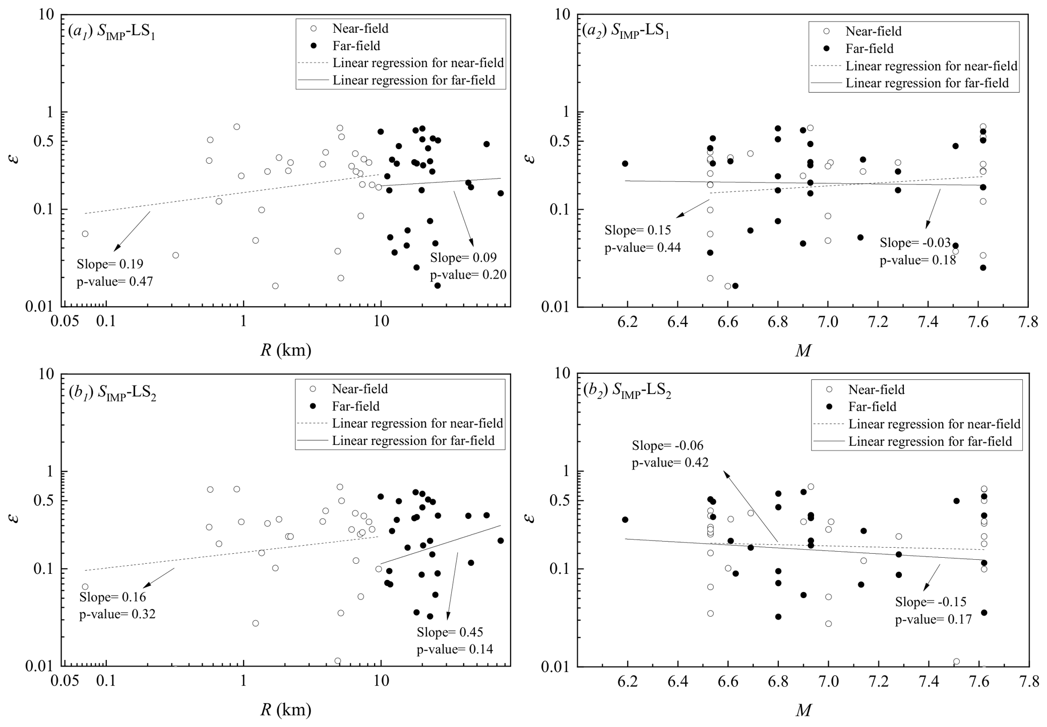
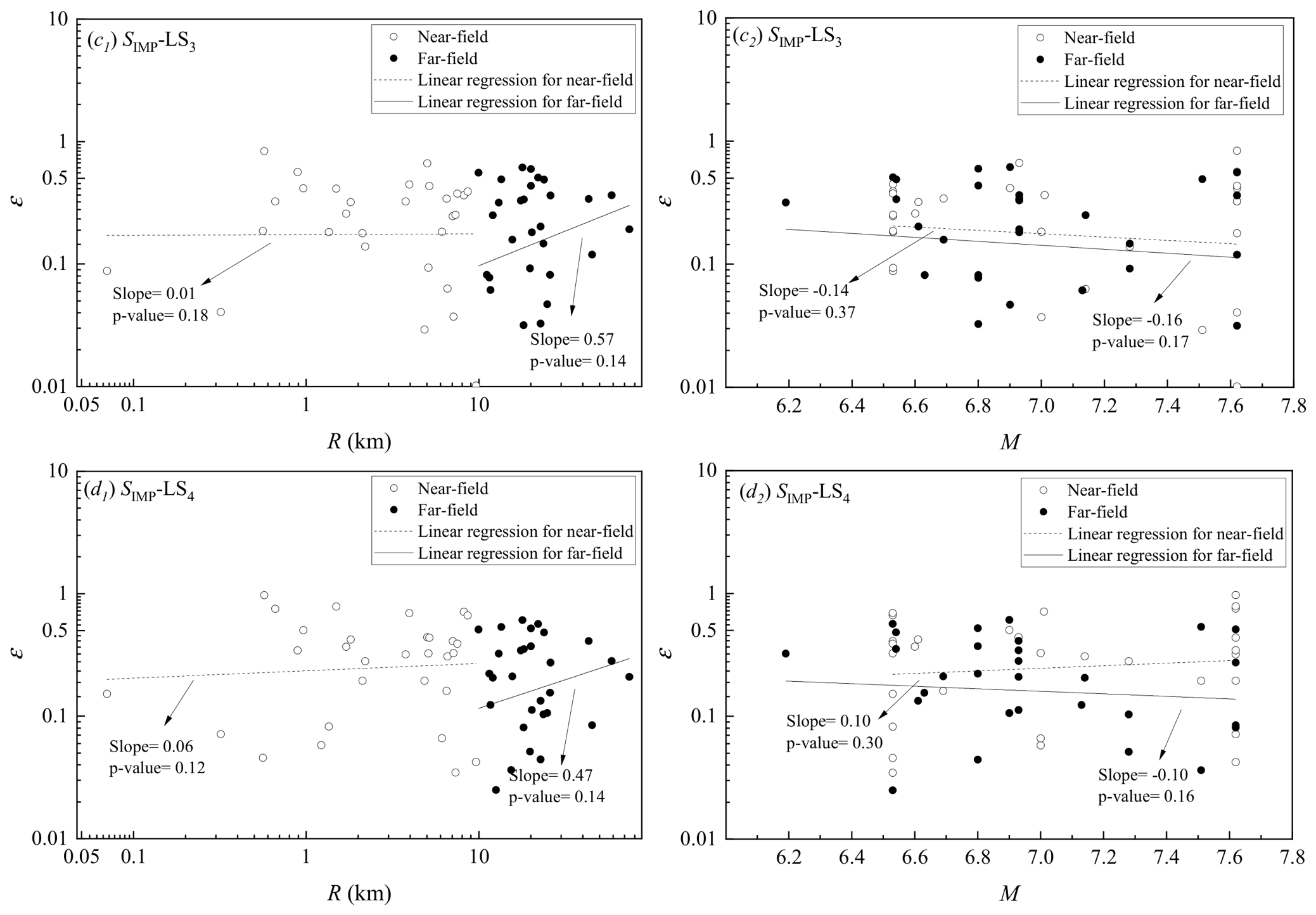
In addition to the low seismic uncertainty achieved by the optimized intensity measure, which demonstrates its effectiveness in characterizing ground motion intensity, a high-quality intensity measure should also exhibit good sufficiency and scaling robustness (Tothong and Luco, 2007 [70]; Bojórquez and Iervolino, 2011 [66]). The sufficiency of a ground motion intensity measure refers to the conditional independence between engineering demand parameters and seismological variables (such as magnitude M and source-to-site distance R given a specified intensity measure). This property is evaluated by performing linear regression between the residual error ln(ε|IM) and M or ln(R), as expressed in Equation (15) (Tothong and Luco, 2007 [70]; Luco and Cornell, 2007 [71]). The p-value obtained from the regression analysis is used to assess the statistical significance of the variables. When the p-value is greater than 0.05, the intensity measure is considered sufficient.

$$\ln (DM)=\ln a+b\ln (IM)+\ln (\epsilon |IM)$$

(15)

where coefficients a and b are determined through linear regression analysis, and ε|IM denotes the random error term.

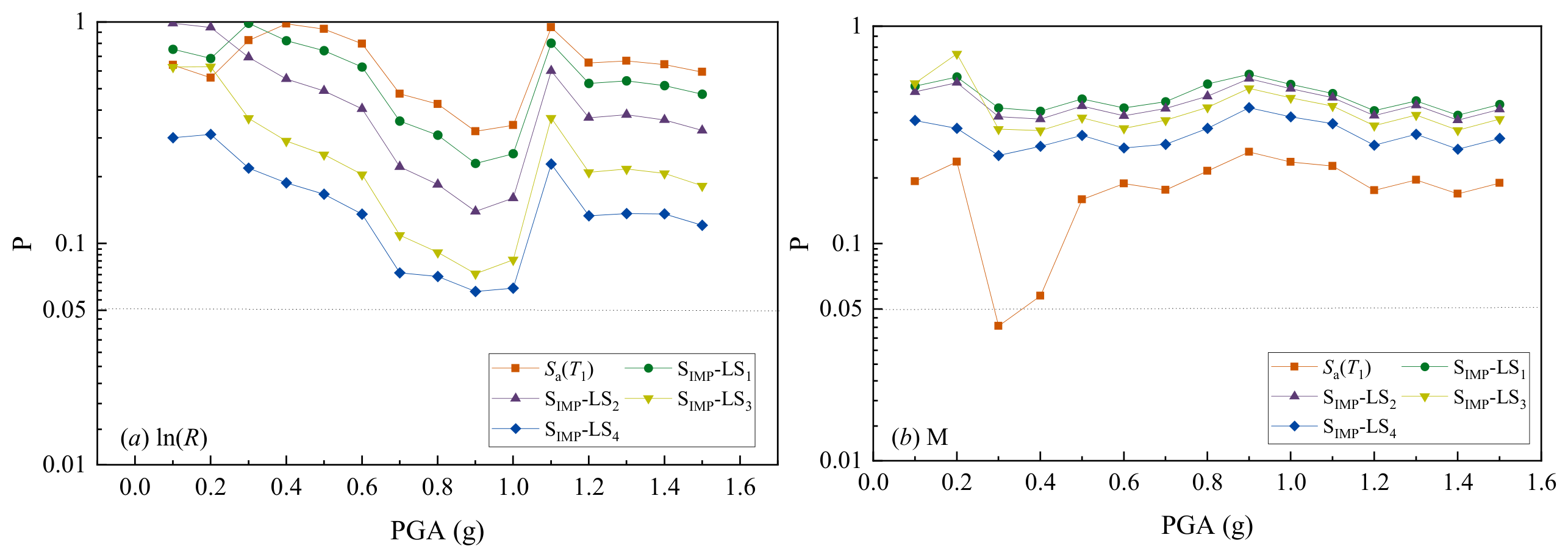
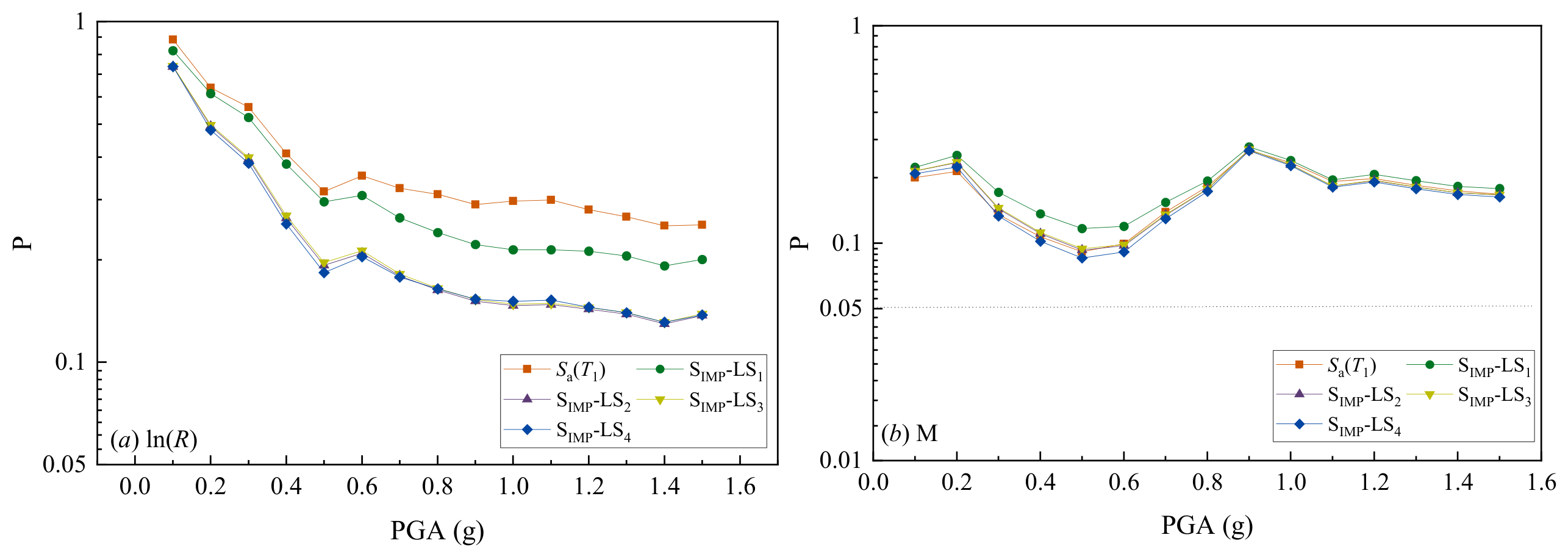
To better evaluate the performance of the proposed spectral acceleration-based intensity measure, this study compares the improved S_IMP index with S_a(T₁) under different PGA levels. Taking PGA = 1.5 g as an example, the ground motion intensities shown in Figure 9 and Figure 10 are transformed into intensity measures described by S_a(T₁). A linear regression between ln(S_a(T₁)) and ln(D_O) is first performed, and the resulting residual ln(ε|S_a(T₁)) is further regressed against seismic parameters M and ln(R), as shown in Figure 18. Similarly, after converting the scaled ground motions at PGA = 1.5 g into the proposed S_IMP measure, the residual ln(ε|S_IMP) is regressed against M and ln(R), as illustrated in Figure 19. It can be observed that, at PGA = 1.5 g, both S_a(T₁) and S_IMP yield p-values greater than 0.05, indicating that both intensity measures satisfy the sufficiency requirement at this intensity level. Figure 20 and Figure 21 further present the p-values obtained from S_a(T₁) and S_IMP across 15 PGA levels ranging from 0.1 g to 1.5 g. The results show that the p-values of S_IMP consistently remain above 0.05, confirming its sufficiency across all intensity levels. In contrast, S_a(T₁) exhibits p-values below 0.05 under near-field conditions when the PGA is scaled to 0.3 g, indicating a violation of sufficiency. Therefore, from the perspective of sufficiency, the proposed S_IMP measure is more suitable for RCS frame structures.

5.6. Robustness of the S_IMP Intensity Measure

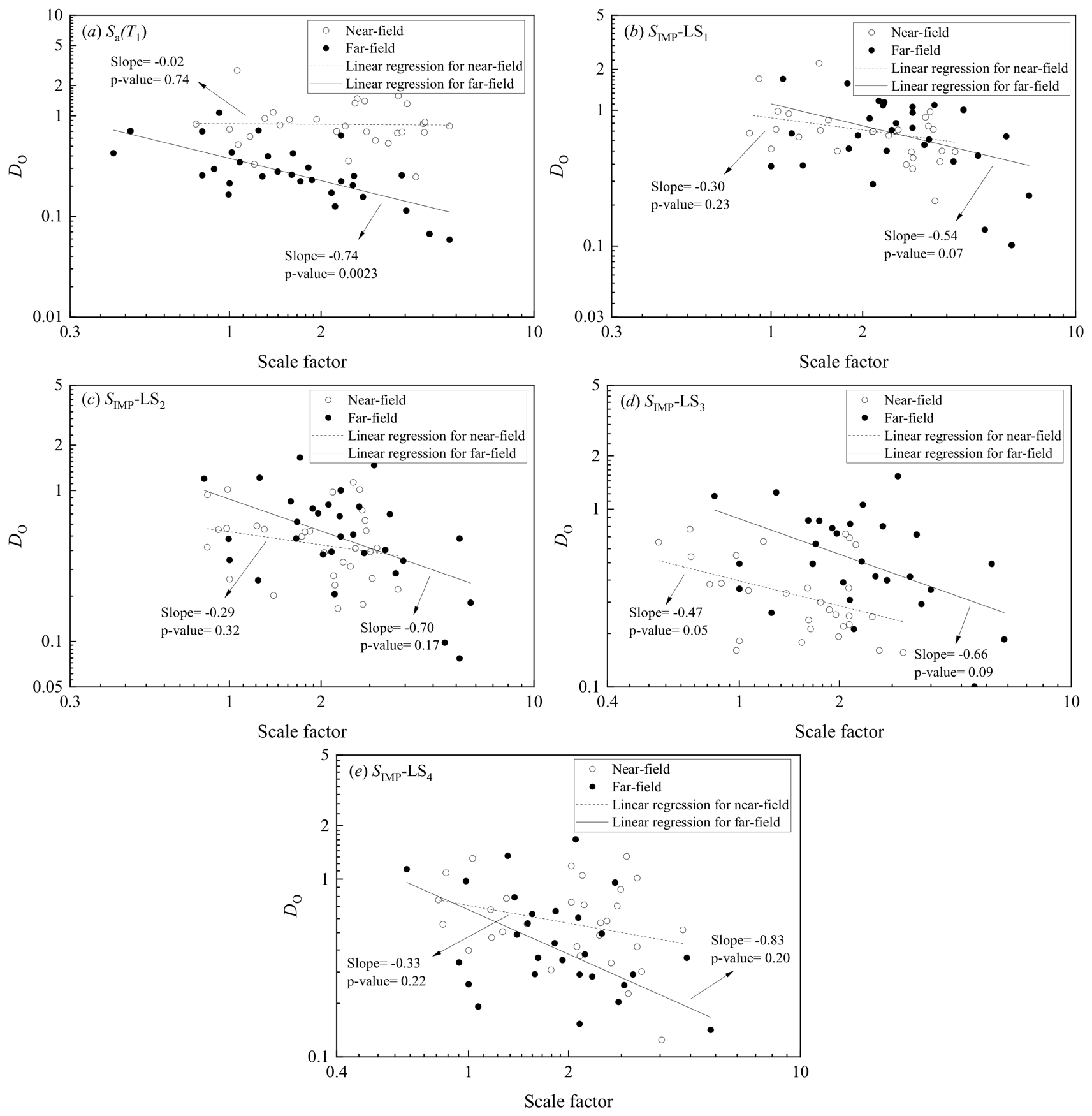
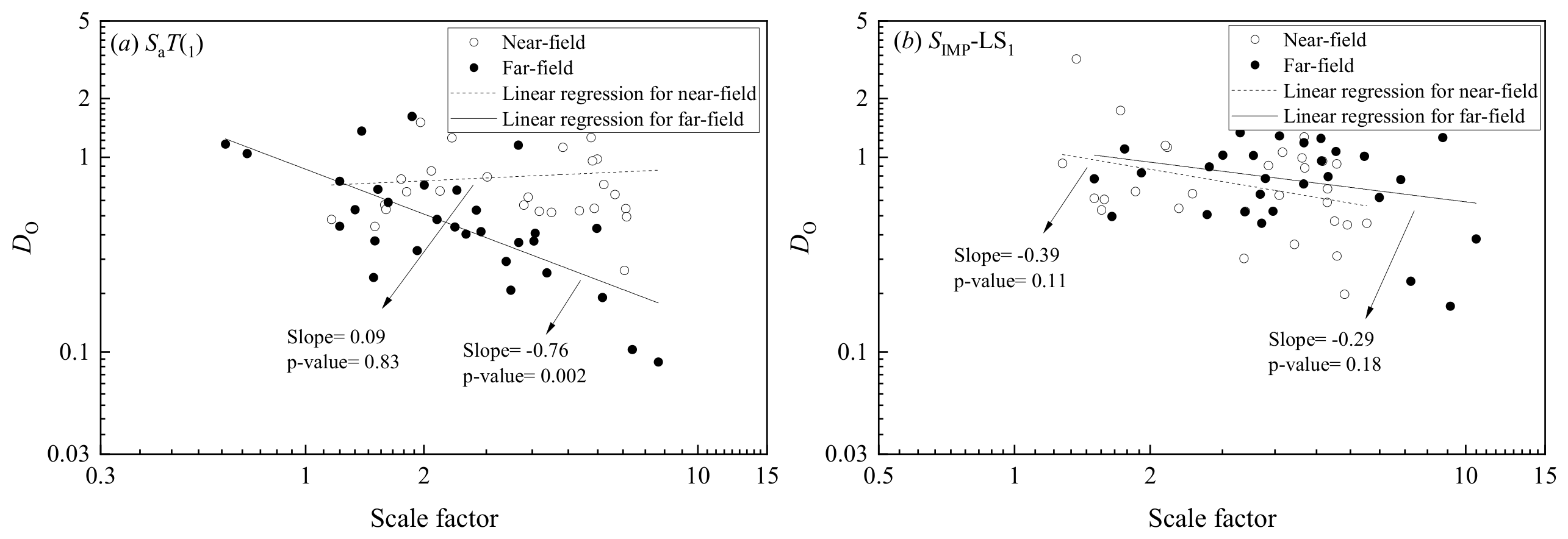
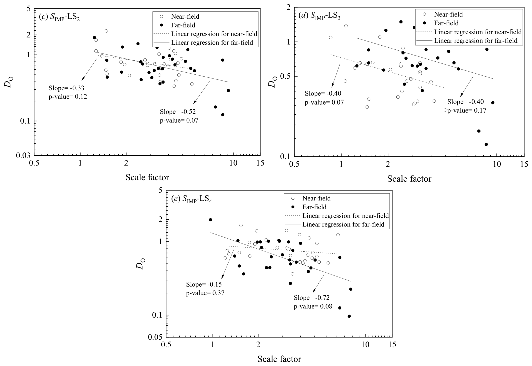
The scaling robustness of a ground motion intensity measure ensures that, when seismic records are scaled to the same intensity level, no systematic trend exists between structural responses and scaling factors (Tothong and Luco, 2007 [70]; Bojórquez and Iervolino, 2011 [66]; Zhang et al., 2018a [72], 2018b [48]). This property is evaluated by performing a log-linear regression between structural response and the scaling factor. When the slope of the regression line is close to zero, the relationship is considered unbiased, indicating that the intensity measure is robust to amplitude scaling. In practice, the p-value of the regression coefficient is commonly used for assessment. When the p-value is greater than 0.05, the intensity measure is considered to satisfy scaling robustness.

Taking the six-story RCS frame structure investigated in this study as an example, a scaling robustness analysis of the proposed S_IMP intensity measure is conducted and compared with the first-mode spectral acceleration S_a(T₁). To drive the structure into a deeper nonlinear response regime, the ground motions with the highest PGA values from both near-field and far-field categories in Table 3 are selected as reference records. Specifically, the far-field ground motion No.22 NORTHR/TAR360 with PGA = 0.99 g is used as the scaling target for the far-field case, while the near-field ground motion No.1 SFERN/PUL164 with PGA = 1.22 g is adopted as the reference record for the near-field case. When other ground motions are scaled to the same S_a(T₁) and S_IMP levels, most records exhibit relatively large scaling factors. To further investigate this effect, the reference ground motions are additionally amplified by a factor of 1.5, resulting in a proportional increase in the scaling factors for all records. Figure 22 and Figure 23 illustrate the relationship between seismic damage D_O and the scaling factor under the two considered cases. As shown in Figure 23, the structure experiences more severe damage under seismic excitation. Notably, in both cases, the p-values associated with S_IMP remain greater than 0.05, confirming its scaling robustness. However, under far-field conditions, the p-value of S_a(T₁) remains below 0.05. From the perspective of scaling robustness, S_IMP and similar adjusted-period-based intensity measures are therefore more suitable for RCS frame structures.

6. Conclusions

This study adopts a dual-parameter damage model based on deformation and energy to conduct seismic fragility analysis of a six-story RCS frame structure. The damage evolution characteristics of the structure under near-field and far-field ground motions are investigated, and fragility analyses based on the dual-parameter damage model are performed for different damage limit states. Furthermore, the applicability of 22 seismic intensity measures in fragility assessment under different damage limit states is examined. Finally, an improved spectral acceleration-based intensity measure (S_IMP) is developed using the SA algorithm. Its sufficiency and scaling robustness are subsequently evaluated. The main conclusions are summarized as follows:

• There are significant differences in the damage effects of near-field and far-field ground motions on RCS frame structures. The pulse characteristics and high-energy duration of near-field ground motions lead to greater dispersion in structural damage and a faster damage evolution rate. At the same PGA level, the damage severity induced by near-field ground motions is significantly higher than that caused by far-field motions. Structural damage is concentrated in the lower stories (1–2 stories), with joint regions identified as the critical damage zones. The peak bending moments and rotation demands in these regions under near-field ground motions are approximately twice those observed under far-field ground motions.
• Among peak-based seismic intensity measures, PGD consistently performs poorly under both near-field and far-field ground motions, showing inferior performance compared with PGA and PGV. When structural period characteristics are considered, S_a(T₁) and S_d(T₁) outperform their corresponding peak-based counterparts (PGA and PGD). Spectral acceleration-based intensity measures that incorporate period softening effects and higher-mode contributions exhibit superior performance under both types of ground motions. In particular, the intensity measures accounting for period softening effects demonstrate higher stability across different damage limit states, such as S* and IM-CR.
• After optimizing the period coefficient n and weighting factor α of the intensity measure using the SA algorithm, the reduction in β_RTR ranges from 8.7% to 38.1%. The improvement is more pronounced under far-field ground motion conditions, and optimal parameter combinations are obtained for all damage limit states. The results of the sufficiency and scaling robustness verification show that the optimized intensity measure yields p-values greater than 0.05 across the entire PGA range. It is conditionally independent of earthquake magnitude and epicentral distance, and no significant trend is observed between structural response and scaling factor. These findings demonstrate that the proposed measure exhibits good stability and applicability.

Despite the findings presented, this study has several limitations that warrant further investigation. A two-dimensional planar frame model was adopted, which simplifies the three-dimensional behavior of actual structures. The selected ground motion records have limitations in both quantity and characteristic coverage, and only unidirectional seismic input was considered without accounting for the influence of multi-directional excitations. The applicability of the optimized S_IMP intensity measure to RCS buildings with different heights, span arrangements and seismic fortification levels requires further validation.

References

1. Guo, Z.; Zhu, Q.; Liu, Y.; Huang, Q. Experimental Study on Seismic Behavior of a New Type of Prefabricated RC Column-Steel Beam Frame Connections. Jianzhu Jiegou Xuebao (J. Build. Struct.) 2012, 33, 98–105. (In Chinese) [Google Scholar]
2. Ling, Y.; Xu, J.; Guo, Z.; Wen, X. A Study on Static Behavior of New Reinforced Concrete Column-Steel Beam Composite Joints. J. Asian Archit. Build. Eng. 2021, 20, 44–60. [Google Scholar] [CrossRef] [Scilit]
3. Men, J.; Xiong, L.; Wang, J.; Fan, G. Effect of Different RC Slab Widths on the Behavior of Reinforced Concrete Column and Steel Beam-Slab Subassemblies. Eng. Struct. 2021, 229, 111639. [Google Scholar] [CrossRef] [Scilit]
4. Moehle, J.; Deierlein, G.G. A Framework Methodology for Performance-Based Earthquake Engineering. In Proceedings of the 13th World Conference on Earthquake Engineering, Vancouver, BC, Canada, 1–6 August 2004; Paper No. 679. p. 12. [Google Scholar]
5. Stewart, J.P.; Chiou, S.-J.; Bray, J.D.; Graves, R.W.; Somerville, P.G.; Abrahamson, N.A. Ground Motion Evaluation Procedures for Performance-Based Design. Soil Dyn. Earthq. Eng. 2002, 22, 765–772. [Google Scholar] [CrossRef] [Scilit]
6. Zhang, Y.; Xia, B.; Guo, X.; Sun, B.; Hu, D.; Wei, Y. Genetic Algorithm-Enhanced Housner Intensity Measure for Seismic Vulnerability Analysis of Reinforced Concrete Column-Steel Beam (RCS) Frame Structure. Soil Dyn. Earthq. Eng. 2025, 193, 109320. [Google Scholar] [CrossRef] [Scilit]
7. Ebrahimian, H.; Jalayer, F.; Lucchini, A.; Mollaioli, F.; Manfredi, G. Preliminary Ranking of Alternative Scalar and Vector Intensity Measures of Ground Shaking. Bull. Earthq. Eng. 2015, 13, 2805–2840. [Google Scholar] [CrossRef] [Scilit]
8. Kostinakis, K.; Fontara, I.-K.; Athanatopoulou, A.M. Scalar Structure-Specific Ground Motion Intensity Measures for Assessing the Seismic Performance of Structures: A Review. J. Earthq. Eng. 2018, 22, 630–665. [Google Scholar] [CrossRef] [Scilit]
9. Du, M. Study on Ground Motion Intensity Measures and Seismic Performance Assessment of Elevated Long-Span Aqueduct Structures in High-Intensity Seismic Zones. Doctoral Dissertation, Tianjin University, Tianjin, China, 2024. (In Chinese) [Google Scholar]
10. Tidke, A.R.; Adhikary, S. Optimal Intensity Measure Selection and Probabilistic Seismic Demand Models for Dam-Reservoir-Layered Foundation System. In Structures; Elsevier: Amsterdam, The Netherlands, 2022; Volume 37, pp. 318–337. [Google Scholar]
11. Pinzón, L.A.; Vargas-Alzate, Y.F.; Pujades, L.G.; Diaz, S.A. A Drift-Correlated Ground Motion Intensity Measure: Application to Steel Frame Buildings. Soil Dyn. Earthq. Eng. 2020, 132, 106096. [Google Scholar] [CrossRef] [Scilit]
12. Ozmen, H.B. Developing Hybrid Parameters for Measuring Damage Potential of Earthquake Records: Case for RC Building Stock. Bull. Earthq. Eng. 2017, 15, 3083–3101. [Google Scholar] [CrossRef] [Scilit]
13. Song, H.F. Seismic Performance Study of RCS Composite Structures with Semi-Rigid Beam-Column Connections. Master’s Thesis, Jiangsu University of Science and Technology, Zhenjiang, China, 2016. (In Chinese) [Google Scholar]
14. Belleri, A. Displacement Based Design for Precast Concrete Frames with Not-Emulative Connections. Eng. Struct. 2017, 141, 228–240. [Google Scholar] [CrossRef] [Scilit]
15. Park, Y.J.; Ang, A.H.-S. Mechanistic Seismic Damage Model for Reinforced Concrete. J. Struct. Eng. 1985, 111, 722–739. [Google Scholar] [CrossRef] [Scilit]
16. Kunnath, S.K.; Reinhorn, A.M.; Abel, J.F. A Computational Tool for Evaluation of Seismic Performance of Reinforced Concrete Buildings. Comput. Struct. 1991, 41, 157–173. [Google Scholar] [CrossRef] [Scilit]
17. Ou, J.; Niu, D.; Wang, G. Loss Estimation and Optimal Design of Nonlinear Reinforced Concrete Seismic Structures. China Civ. Eng. J. 1993, 26, 14–21. (In Chinese) [Google Scholar] [CrossRef]
18. Riddell, R. On Ground Motion Intensity Indices. Earthq. Spectra 2007, 23, 147–173. [Google Scholar] [CrossRef] [Scilit]
19. Ye, L.; Ma, Q.; Miao, Z.; Guan, H.; Zhuge, Y. Numerical and Comparative Study of Earthquake Intensity Indices in Seismic Analysis. Struct. Des. Tall Spec. Build. 2013, 22, 362–381. [Google Scholar] [CrossRef] [Scilit]
20. Zhou, Y.; Li, M. An Area-Based Intensity Measure for Incremental Dynamic Analysis. J. Asian Archit. Build. Eng. 2015, 14, 451–457. [Google Scholar] [CrossRef] [Scilit]
21. Yang, C.; Xie, L.; Li, A.; Jia, J.; Zeng, D. Ground Motion Intensity Measures for Seismically Isolated RC Tall Buildings. Soil Dyn. Earthq. Eng. 2019, 125, 105727. [Google Scholar] [CrossRef] [Scilit]
22. Zhang, Y.; Zhang, J.; Zhang, J.; Zheng, K.; Wei, Y. Comparative Analysis of Seismic Response and Vulnerability of Laminated Bamboo Frame Structure Under Near-Field and Far-Field Earthquake Actions. In Structures; Elsevier: Amsterdam, The Netherlands, 2024; Volume 69, p. 107321. [Google Scholar]
23. Lazaridis, P.C.; Kavvadias, I.E.; Demertzis, K.; Iliadis, L.; Vasiliadis, L.K. Structural Damage Prediction of a Reinforced Concrete Frame under Single and Multiple Seismic Events Using Machine Learning Algorithms. Appl. Sci. 2022, 12, 3845. [Google Scholar] [CrossRef] [Scilit]
24. Massumi, A.; Gholami, F. The Influence of Seismic Intensity Parameters on Structural Damage of RC Buildings Using Principal Components Analysis. Appl. Math. Modell. 2016, 40, 2161–2176. [Google Scholar] [CrossRef] [Scilit]
25. Zhang, Z.; Ke, X. A New Simulated Annealing Algorithm for Terminal Allocation. In Proceedings of the 3rd WSEAS International Conference on Circuits, Systems, Signal and Telecommunications; World Scientific and Engineering Academy and Society (WSEAS): Stevens Point, WI, USA, 2009; pp. 47–50. [Google Scholar]
26. Wu, X.M.; Li, G.X.; Shan, D.B.; Yu, G.B. RBF Neural Network Arithmetic and Applications in Surface Interpolation Reconstruction. Key Eng. Mater. 2011, 460–461, 575–580. [Google Scholar] [CrossRef] [Scilit]
27. Weng, S.; Yu, C.; Liu, Y. Automatic Design Method for RF Front-End Based on Simulated Annealing Arithmetic. In Proceedings of the 2022 IEEE MTT-S International Microwave Workshop Series on Advanced Materials and Processes for RF and THz Applications (IMWS-AMP); IEEE: New York, NY, USA, 2022; pp. 1–3. [Google Scholar]
28. Shahandashti, S.M.; Pudasaini, B. Proactive Seismic Rehabilitation Decision-Making for Water Pipe Networks Using Simulated Annealing. Nat. Hazards Rev. 2019, 20, 04019003. [Google Scholar] [CrossRef] [Scilit]
29. Pudasaini, B.; Shahandashti, M. Seismic Rehabilitation Optimization of Water Pipe Networks Considering Spatial Variabilities of Demand Criticalities and Seismic Ground Motion Intensities. J. Infrastruct. Syst. 2021, 27, 04021028. [Google Scholar] [CrossRef] [Scilit]
30. Roy, A.; Shahandashti, M. Proactive Seismic Rehabilitation Decision Making for a Road Network Considering Multiple Assets’ Performance Uncertainties. In Proceedings of the International Conference on Transportation and Development 2024; American Society of Civil Engineers: Atlanta, Georgia, 2024; pp. 230–241. [Google Scholar]
31. Mase, L.Z.; Irsyam, M.; Gustiparani, D.; Noptapia, A.N.; Syahbana, A.J.; Soebowo, E. Identification of Bedrock Depth along a Downstream Segment of Muara Bangkahulu River, Bengkulu City, Indonesia. Bull. Eng. Geol. Environ. 2024, 83, 93. [Google Scholar] [CrossRef] [Scilit]
32. GB/T50010-2010; Standard for Design of Concrete Structures (2024 Edition). China Architecture & Building Press: Beijing, China, 2024. (In Chinese)
33. GB/T50011-2010; Standard for Seismic Design of Buildings (2024 Edition). China Architecture & Building Press: Beijing, China, 2024. (In Chinese)
34. GB 50017-2017; Standard for Design of Steel Structures. China Architecture & Building Press: Beijing, China, 2017. (In Chinese)
35. Sheikh, T.M. Moment Connections Between Steel Beams and Concrete Columns; The University of Texas at Austin: Austin, TX, USA, 1987. [Google Scholar]
36. Deierlein, G.G. Design of Moment Connections for Composite Framed Structures; The University of Texas at Austin: Austin, TX, USA, 1988. [Google Scholar]
37. Sheikh, T.M.; Deierlein, G.G.; Yura, J.A.; Jirsa, J.O. Beam-Column Moment Connections for Composite Frames: Part 1. J. Struct. Eng. 1989, 115, 2858–2876. [Google Scholar] [CrossRef] [Scilit]
38. Deierlein, G.G.; Sheikh, T.M.; Yura, J.A.; Jirsa, J.O. Beam-Column Moment Connections for Composite Frames: Part 2. J. Struct. Eng. 1989, 115, 2877–2896. [Google Scholar] [CrossRef] [Scilit]
39. Li, X.R.; Qin, B. Steel Structure Connection Node Design Manual; China Construction Industry Press: Beijing, China, 2019. (In Chinese) [Google Scholar]
40. Nishiyama, I.; Kuramoto, H.; Noguchi, H. Guidelines: Seismic Design of Composite Reinforced Concrete and Steel Buildings. J. Struct. Eng. 2004, 130, 336–342. [Google Scholar] [CrossRef] [Scilit]
41. Lucchini, A.; Mollaioli, F.; Monti, G. Intensity Measures for Response Prediction of a Torsional Building Subjected to Bi-Directional Earthquake Ground Motion. Bull. Earthq. Eng. 2011, 9, 1499–1518. [Google Scholar] [CrossRef] [Scilit]
42. Kostinakis, K.; Athanatopoulou, A.; Morfidis, K. Correlation between Ground Motion Intensity Measures and Seismic Damage of 3D R/C Buildings. Eng. Struct. 2015, 82, 151–167. [Google Scholar] [CrossRef] [Scilit]
43. Yassin, M.H.M. Nonlinear Analysis of Prestressed Concrete Structures Under Monotonic and Cycling Loads. Ph.D. Thesis, University of California Berkeley, Berkeley, CA, USA, 1994. [Google Scholar]
44. Filippou, F.C.; Popov, E.P.; Bertero, V.V. Effects of Bond Deterioration on Hysteretic Behavior of Reinforced Concrete Joints; Report EERC 83-19; Earthquake Engineering Research Center, University of California Berkeley: Berkeley, CA, USA, 1983. [Google Scholar]
45. Aloisio, A.; Contento, A.; Alaggio, R.; Briseghella, B.; Fragiacomo, M. Probabilistic assessment of a light-timber frame shear wall with variable pinching under repeated earthquakes. J. Struct. Eng. 2022, 148, 04022178. [Google Scholar] [CrossRef] [Scilit]
46. Shahnewaz, M.; Pan, Y.; Shahria Alam, M.; Tannert, T. Seismic fragility estimates for cross-laminated timber platform building. J. Struct. Eng. 2020, 146, 04020256. [Google Scholar] [CrossRef] [Scilit]
47. Mitra, N. Pinching4 Uniaxial Material Model. Available online: https://opensees.berkeley.edu/wiki/index.php/Pinching4_Material (accessed on 20 April 2026).
48. Zhang, Y.; He, Z.; Yang, Y. A Spectral-Velocity-Based Combination-Type Earthquake Intensity Measure for Super High-Rise Buildings. Bull. Earthq. Eng. 2018, 16, 643–677. [Google Scholar] [CrossRef] [Scilit]
49. Zhang, Y.; He, Z. Appropriate Ground Motion Intensity Measures for Estimating the Earthquake Demand of Floor Acceleration-Sensitive Elements in Super High-Rise Buildings. Struct. Infrastruct. Eng. 2019, 15, 467–483. [Google Scholar] [CrossRef] [Scilit]
50. Ancheta, T.D.; Darragh, R.B.; Stewart, J.P.; Seyhan, E.; Silva, W.J.; Chiou, B.S.-J.; Wooddell, K.E.; Graves, R.W.; Kottke, A.R.; Boore, D.M.; et al. NGA-West2 Database. Earthq. Spectra 2014, 30, 989–1005. [Google Scholar] [CrossRef] [Scilit]
51. Federal Emergency Management Agency (FEMA). Quantification of Building Seismic Performance Factors; FEMA P-695; Federal Emergency Management Agency (FEMA): Washington, DC, USA, 2009.
52. Baker, J.W. Quantitative Classification of Near-Fault Ground Motions Using Wavelet Analysis. Bull. Seismol. Soc. Am. 2007, 97, 1486–1501. [Google Scholar] [CrossRef] [Scilit]
53. Kunnath, S.K.; Reinhorn, A.M.; Lobo, R.F. IDARC Version 3.0: A Program for the Inelastic Damage Analysis of Reinforced Concrete Structures; National Center for Earthquake Engineering Research: Buffalo, NY, USA, 1992. [Google Scholar]
54. Men, J.; Zhang, Q.; Xu, C.; Shi, Q. Seismic Damage Assessment of RCS Hybrid Frame Structures Based on an Improved Park-Ang Two-Parameter Model. Eng. Mech. 2020, 37, 133–143. (In Chinese) [Google Scholar]
55. Kunnath, S.K.; Reinhorn, A.M.; Park, Y.J. Analytical Modeling of Inelastic Seismic Response of R/C Structures. J. Struct. Eng. 1990, 116, 996–1017. [Google Scholar] [CrossRef] [Scilit]
56. Ma, H.; Zhang, N.; Liu, Y.; Wang, Z.; Liang, J. Seismic Damage Study on Composite Frame Joints of Steel Reinforced Recycled Concrete Columns and Steel Beams. Chin. J. Appl. Mech. 2018, 35, 616–623. (In Chinese) [Google Scholar]
57. Song, H.F.; Zhang, Y.B.; Pan, Z.H.; Zhou, Z.B. Study on Seismic Damage Model of Edge Joints of Reinforced Concrete Column-Steel Beam Composite Structure. Build. Struct. 2016, 46, 55–60. (In Chinese) [Google Scholar] [CrossRef]
58. Baker, J.W. Efficient Analytical Fragility Function Fitting Using Dynamic Structural Analysis. Earthq. Spectra 2015, 31, 579–599. [Google Scholar] [CrossRef] [Scilit]
59. Nuttli, O.W. The Relation of Sustained Maximum Ground Acceleration and Velocity to Earthquake Intensity and Magnitude; US Army Engineer Waterways Experiment Station: Vicksburg, MS, USA, 1979. [Google Scholar]
60. Von Thun, J.L.; Roehm, L.H.; Scott, G.A.; Wilson, J.A. Earthquake Ground Motions for Design and Analysis of Dams. In Earthquake Engineering and Soil Dynamics II: Recent Advances in Ground-Motion Evaluation; ASCE: New York, NY, USA, 1988; pp. 1–12. [Google Scholar]
61. Shome, N.; Cornell, C.A. Probabilistic Seismic Demand Analysis of Non-Linear Structures; Stanford University: Stanford, CA, USA, 1999. [Google Scholar]
62. Kazantzi, A.K.; Vamvatsikos, D. Intensity Measure Selection for Vulnerability Studies of Building Classes. Earthq. Eng. Struct. Dyn. 2015, 44, 2677–2694. [Google Scholar] [CrossRef] [Scilit]
63. Housner, G.W. Spectrum Intensities of Strong-Motion Earthquakes. In Proceedings of the Symposium on Earthquake and Blast Effects on Structures; Earthquake Engineering Research Institute: Los Angeles, CA, USA, 1952; pp. 20–36. [Google Scholar]
64. Cordova, P.P.; Deierlein, G.G.; Mehanny, S.S.; Cornell, C.A. Development of a Two-Parameter Seismic Intensity Measure and Probabilistic Assessment Procedure. In Proceedings of the Second US-Japan Workshop on Performance-Based Earthquake Engineering Methodology for Reinforced Concrete Building Structures, Sapporo, Japan, 11–13 September 2001. [Google Scholar]
65. Mehanny, S.S. A Broad-Range Power-Law Form Scalar-Based Seismic Intensity Measure. Eng. Struct. 2009, 31, 1354–1368. [Google Scholar] [CrossRef] [Scilit]
66. Bojórquez, E.; Iervolino, I. Spectral Shape Proxies and Nonlinear Structural Response. Soil Dyn. Earthq. Eng. 2011, 31, 996–1008. [Google Scholar] [CrossRef] [Scilit]
67. Vamvatsikos, D.; Cornell, C.A. Developing Efficient Scalar and Vector Intensity Measures for IDA Capacity Estimation by Incorporating Elastic Spectral Shape Information. Earthq. Eng. Struct. Dyn. 2005, 34, 1573–1600. [Google Scholar] [CrossRef] [Scilit]
68. Lin, L.; Naumoski, N.; Saatcioglu, M.; Foo, S. Improved Intensity Measures for Probabilistic Seismic Demand Analysis. Part 1: Development of Improved Intensity Measures. Can. J. Civ. Eng. 2011, 38, 79–88. [Google Scholar] [CrossRef] [Scilit]
69. Rintoul, M.D.; Torquato, S. Reconstruction of the Structure of Dispersions. J. Colloid Interface Sci. 1997, 186, 467–476. [Google Scholar] [CrossRef] [Scilit] [PubMed]
70. Tothong, P.; Luco, N. Probabilistic Seismic Demand Analysis Using Advanced Ground Motion Intensity Measures. Earthq. Eng. Struct. Dyn. 2007, 36, 1837–1860. [Google Scholar] [CrossRef] [Scilit]
71. Luco, N.; Cornell, C.A. Structure-Specific Scalar Intensity Measures for Near-Source and Ordinary Earthquake Ground Motions. Earthq. Spectra 2007, 23, 357–392. [Google Scholar] [CrossRef] [Scilit]
72. Zhang, Y.; He, Z.; Lu, W.; Yang, Y. A Spectral-Acceleration-Based Linear Combination-Type Earthquake Intensity Measure for High-Rise Buildings. J. Earthq. Eng. 2018, 22, 1479–1508. [Google Scholar] [CrossRef] [Scilit]
Figure 1. Structural side elevations and modeling strategies.
Buildings 16 02185 g001
Figure 2. Schematic diagrams of joint design.
Buildings 16 02185 g002
Figure 3. Comparison of loading and numerical simulation results for beam–column joints in RCS frame structures.
Buildings 16 02185 g003
Figure 4. Acceleration response spectra of near-field and far-field ground motions.
Buildings 16 02185 g004
Figure 5. Damage evolution of the beam at the second floor between grid A and grid B and the base column at grid A under the near-field ground motion SFERN/PUL164.
Buildings 16 02185 g005
Figure 6. Seismic damage distribution along stories.
Buildings 16 02185 g006
Figure 7. Moment–rotation response at column-end regions under near-field and far-field ground motions at 0.4 g.
Buildings 16 02185 g007
Figure 8. Moment–rotation response at beam-end regions under near-field and far-field ground motions at 0.4 g.
Buildings 16 02185 g008
Figure 9. Fragility curves for the RCS structure under near-field seismic excitations.
Buildings 16 02185 g009
Figure 10. Fragility curves for the RCS structure under far-field seismic excitations.
Buildings 16 02185 g010
Figure 11. βRTR values for different damage limit states under near-field seismic motions.
Buildings 16 02185 g011
Figure 12. βRTR values for different damage limit states under far-field seismic motions.
Buildings 16 02185 g012
Figure 13. Fragility curves described using IM-CR under near-field ground motion across four different damage limit states.
Buildings 16 02185 g013
Figure 14. Fragility curves described using IM-CR under far-field ground motion across four different damage limit states.
Buildings 16 02185 g014
Figure 15. Optimization curve of SIMP parameter selection and corresponding fragility curve standard deviation under near-field ground motion conditions.
Buildings 16 02185 g015aBuildings 16 02185 g015b
Figure 16. Optimization curve of SIMP parameter selection and corresponding fragility curve standard deviation under far-field ground motion conditions.
Buildings 16 02185 g016
Figure 17. Comparison of seismic uncertainty before and after optimization for RCS structures under near-field and far-field ground motions across four damage limit states.
Buildings 16 02185 g017
Figure 18. Regression analysis of the residuals ln(ε|Sa(T1)) against M or ln(R) for estimating DO using Sa(T1) at an intensity level corresponding to PGA = 1.5 g.
Buildings 16 02185 g018
Figure 19. Regression analysis of the residuals ln(ε| SIMP) against M or ln(R) for estimating DO using SIMP at an intensity level corresponding to PGA = 1.5 g.
Buildings 16 02185 g019aBuildings 16 02185 g019b
Figure 20. P-values corresponding to Sa(T1) and SIMP when evaluating sufficiency under near-field records.
Buildings 16 02185 g020
Figure 21. P-values corresponding to Sa(T1) and SIMP when evaluating sufficiency under far-field records.
Buildings 16 02185 g021
Figure 22. Relationship between DO and the scaling factor for RCS structures.
Buildings 16 02185 g022
Figure 23. Relationship between Do and the scaling factor amplified by 1.5 for RCS structures.
Buildings 16 02185 g023aBuildings 16 02185 g023b