Simulation of Acoustic Emission Using the Discrete Element Method: Application to Failure Analysis of Masonry Walls Subjected to In-Plane Loading

Abstract

Acoustic emission (AE) is a vital non-destructive technique for monitoring damage in materials, yet its simulation via the Discrete Element Method (DEM) has historically been limited to material-scale analysis. This research presents a novel application of block-based DEM to simulate AE signals in masonry structures at the structural scale under quasi-static in-plane loading. Using a simplified micro-modeling approach, the study first validates the method by monitoring crack initiation and AE energy in single mortar bed joints under tensile and shear conditions. The methodology is then scaled to a large-scale masonry wall panel (1.835 × 1.170 × 0.15 m³) subjected to monotonic shear loading. A critical finding is the influence of local damping; a reduced damping ratio of 0.3 is recommended to preserve the kinetic energy necessary for capturing clear velocity signals. Numerical results show strong agreement with experimental force-displacement and cumulative AE energy curves, confirming the model’s robustness. Furthermore, frequency analysis of the simulated signals successfully distinguishes between tensile and shear failure modes. This study fills a significant gap in the literature by demonstrating that DEM is an effective predictive tool for structural-scale failure analysis and AE monitoring in heterogeneous masonry.

1. Introduction

This study investigates the capability of a velocity-based Discrete Element Method (DEM) approach for simulating acoustic experimental AE measurement behavior. The proposed methodology integrates numerical DEM modeling with experimental results reported in the literature under comparable loading conditions. The published experimental data are used as a reference for validating the DEM simulations and assessing their ability to reproduce AE responses.

Acoustic emission (AE) is a non-destructive testing method used to assess damage in materials and structures. In Civil Engineering, this technique is commonly applied to concrete, metals, and composite materials [1,2,3,4,5] and less frequently to masonry [6]. When a material fails, it releases energy, part of which propagates through elastic waves within the specimen. The surface vibrations resulting from these waves can be captured by piezo-electric sensors, which provide AE signals.

Masonry is a composite material, which is comprised of masonry units (e.g., brick, stone) bonded together with or without mortar. The behavior of masonry depends on the properties of the blocks, the mortar, and the interaction between them. A masonry wall can be constructed using different bonding patterns [7], i.e., the ways in which bricks are laid to create a patterned effect. The type of masonry bonding does not only have a visual effect but affects the mechanical behavior of a masonry wall too. For example, the compressive strength and corresponding strain of full-brick thick Flemish bond prisms is higher and has more deformation than half-brick thick masonry prisms [8]. Another characteristic of masonry is its heterogeneous nature, i.e., consisting of varying mechanical characteristics in each orthogonal direction. This heterogeneous nature presents challenges when applying AE measurements, as the AE signals are attenuated and distorted due to the material’s heterogeneity.

In old and deteriorated low-bond-strength masonry, cracking can occur either at the mortar and/or at the brick to mortar interfaces, as these typically have lower resistance compared to the bricks themselves. In masonry structures, two typical failure modes are observed: in-plane (shear or compression) and out-of-plane bending. Characterizing the mechanical behavior of mortar joints and the brick-to-mortar interface under shear and tension is crucial for understanding the overall behavior of masonry structures. Several experimental studies involved AE monitoring to evaluate the failure mechanisms of mortar joints under shear [9,10,11] and tension [12]. Livitsanos et al. (2019) [10] observed experimentally that the waves propagating in masonry are both attenuated and reflected at the joints between bricks. Consequently, it is essential to consider the presence of interfaces between bricks when simulating AE in masonry structures.

Over the last three decades, significant efforts have been put into the development of numerical models to represent the complex and non-linear behavior of masonry structures subjected to external loads. Such models range from considering masonry as a continuum (e.g., macro-models) to the more detailed ones considering masonry as an assemblage of units and mortar joints (e.g., micro-models). A computational method that is based on the micro-modeling approach and takes into account the heterogeneous nature of masonry is the Discrete or Distinct Element Method (DEM).

The DEM was developed in 1979 by Cundall [13] to solve dynamic equations to simulate granular material flow. This method involves defining the domain using particles connected by interaction laws. Initially, particles were in the form of rigid spheres and represented the motion of granular media such as rock masses and granular soils for applications in geotechnical engineering [14]. In the field of structural engineering and simulating the mechanics of materials like concrete and/or masonry, particularly for large-scale structures, this method remains possible but not practical as it is limited to the number of particles, which could lead to enormous computation efforts and high demands on computing power. To overcome such limitations, DEM was extended over the years, replacing spherical particles with polyhedral ones that are not restricted to a specific geometric shape. This block-based DEM is particularly suited for masonry [15,16,17,18], as it can explicitly simulate the mechanical response of masonry with different bonding patterns. The nature of the contacts between discrete elements in the second approach is more complex than in the first one, as several types of contacts can be generated based on the geometry of the assembled bricks. On the other hand, this method is very practical at the structural scale, as it allows for easy representation of the actual geometry of the bricks and significantly reduces computation time due to the smaller number of discrete elements.

Until today, the simulation of AE using the DEM has only been carried out when simulating a collection of elementary grains primarily for rocks [19,20,21] and concrete [22]. According to the method, use particles that are bonded together in 2D or 3D to represent the specimen under consideration. Most studies have employed particle flow codes combined with the linear parallel bonding model [22]. To analyze the acoustic signal, researchers estimate the number of cracks during loading and compare it to the cumulative acoustic emission counts recorded during experiments. In addition to this approach, Rucka et al. (2023) [22] used the average velocity signal obtained from calculations to analyze the AE of a concrete specimen. Given such limitations, the simulation of AE using the DEM has only been conducted at the material scale or on small test specimens, while no studies have been focused on large-scale structures. Consequently, the question of the feasibility of the DEM to model acoustic emission at the structural scale using the block-based approach remains an open issue.

The discrete nature of masonry can be well reproduced by the discrete element method. The relevance of this method in modeling masonry structures has been demonstrated in several studies [23,24,25,26]. Therefore, a priori, the choice of the DEM can translate the effect of the heterogeneity of masonry in AE well, which is not well reproduced by a continuous medium as supposed in the finite element method. On the other hand, when a joint is broken or when there is a plastic flow in the structure, with the DEM, a significant and rapid increase in kinetic energy in this region allows elastic waves propagating in the structure to be created. This translates the physical phenomenon of AE. When using the DEM to model AE, several questions arise: how can an AE signal be translated through DEM? Can this signal capture the moment/modulus of rupture (MOR) within the structure? If the signal can detect the rupture, is it possible to evaluate the level of damage and the modes of cracking, and can the AE source be located? To address these questions, an extensive research study was conducted and is presented herein.

The aim of this paper is to evaluate the potential of utilizing the discrete element method to accurately simulate the crack initiation and propagation in a masonry wall subjected to in-plane load. Despite the advancements in numerical modeling of Acoustic Emission (AE) [27,28,29], a significant gap remains in simulating these signals at the structural scale for heterogeneous masonry. While existing literature focuses heavily on material-scale particle models for concrete and rock, the computational cost of such methods limits their practical application to large-scale engineering problems. This study fills this gap by providing three primary contributions to the field, including (a) scale transition, (b) damping optimization, and (c) failure mode characterization. In particular, unlike previous DEM models limited to micro-scale specimens, this work proposes a block-based DEM framework capable of simulating AE in structural-scale masonry wall panels (1.8 × 1.1 m). Also, the study identifies a critical numerical threshold for local damping (a = 0.3), offering a specific technical guideline to balance computational stability with the preservation of high-fidelity AE signals—a challenge not addressed in standard DEM applications. Moreover, the study demonstrates that a structural-scale DEM can differentiate between tensile and shear failure signatures, providing a validated ‘virtual testing’ environment for structural health monitoring (SHM) of historical masonry infrastructure. The paper is structured as follows. In the first part, the paper outlines the principles of the discrete element method applied to masonry. Then, the application of DEM to simulate AE is presented. Finally, this method is applied on a masonry wall subjected to quasi-static in-plane loading.

2. Overview of DEM for Modeling Masonry

The 3-DimensionalDistinct Element Codes (3DEC, Version 4.1, Itasca, Minneapolis) were used in this study. The discrete nature of masonry can be effectively modeled using the DEM. Two approaches can be used for discretizing the masonry: the detailed micro-model and the simplified micro-model.

In the detailed micro-model, the actual geometry of the mortar joints is explicitly simulated. This approach accurately captures the real geometry of the mortar, but it can be computationally expensive. In contrast, the simplified micro-model assumes that the contact between blocks can be represented by a contact law to represent the interaction between masonry units, while the mortar is considered a zero-thickness interface.

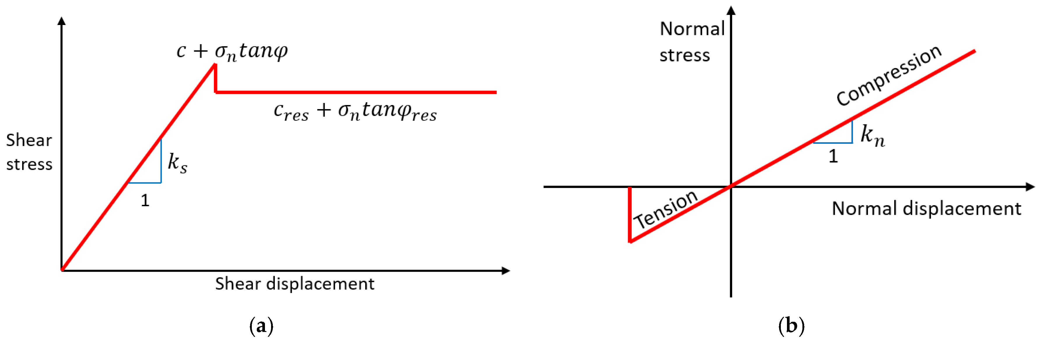
In this study, the simplified micro-modeling approach was employed. In particular, blocks herein representing masonry units are connected by two springs, one in the normal direction and one in the tangential direction. Mortar joints are represented by zero-thickness interfaces, while their elastic response is characterized by two stiffness values: k_n in the normal direction and $k_s$ in the tangential direction. The joint is capable of undergoing shear, tension, and compression. Compression is assumed to be infinitely rigid, while tension follows a linear relationship up to its limit, after which it drops to zero in the post-peak phase.

The shear ($\tau$) behavior of the joint is described by the Mohr–Coulomb law, with parameters including the cohesion strength $\left(c\right)$ friction angle ($\phi$), and dilation angle ($\psi ).$ Under shear, the joint exhibits linear elastic behavior up to its rupture limit, defined by $\tau =c+{\sigma }_{n}tan \phi$. After the peak, the resistance (${\tau }_{res})$ drops to a plateau at a value of ${\tau }_{res}=c_{res}+{\sigma }_{n}tan {\phi }_{res}$, where $c_{res}$ is the residual cohesion, ${\sigma }_n$ is the normal stress, and ${\phi }_{res}$ is the residual frictional angle. The behavior law for the joint under shear and tension is illustrated in Figure 1.

3. Simulation of Acoustic Emission of a Joint Under Shear and Tension Using the DEM

3.1. Geometry and Contact Identification

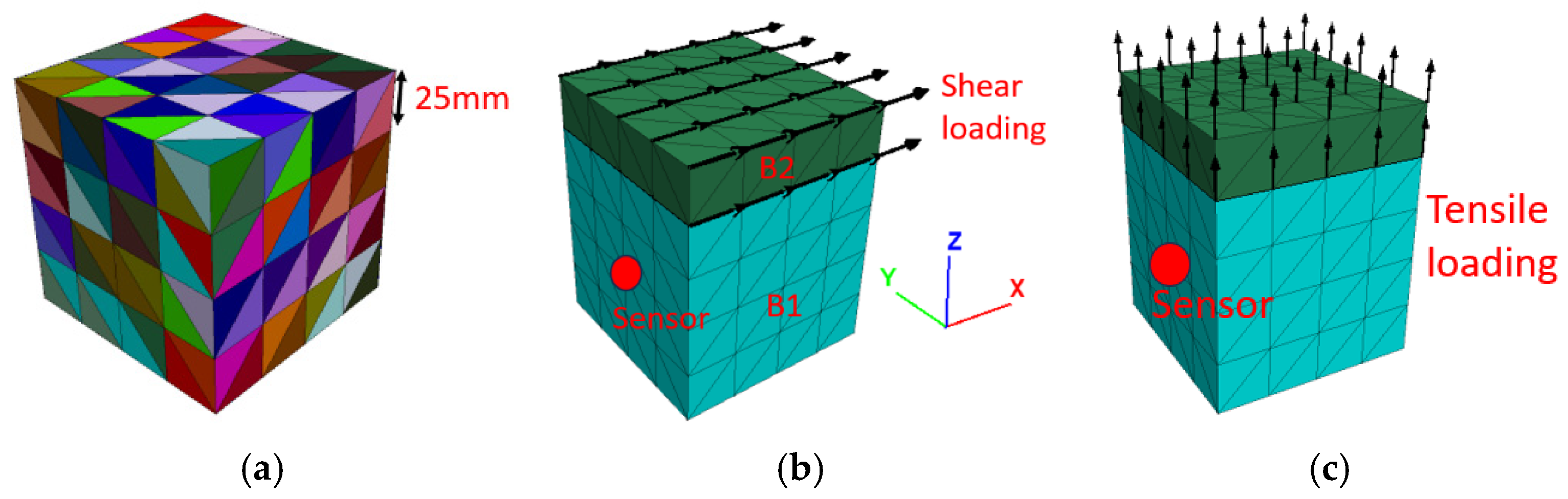
First, a single joint subjected to shear and then direct tension is investigated. In this case, two blocks were considered: Block B1 with dimensions of 0.1 × 0.1 × 0.1 m³ and Block B2 with dimensions of 0.1 × 0.1 × 0.025 m³ (Figure 2).

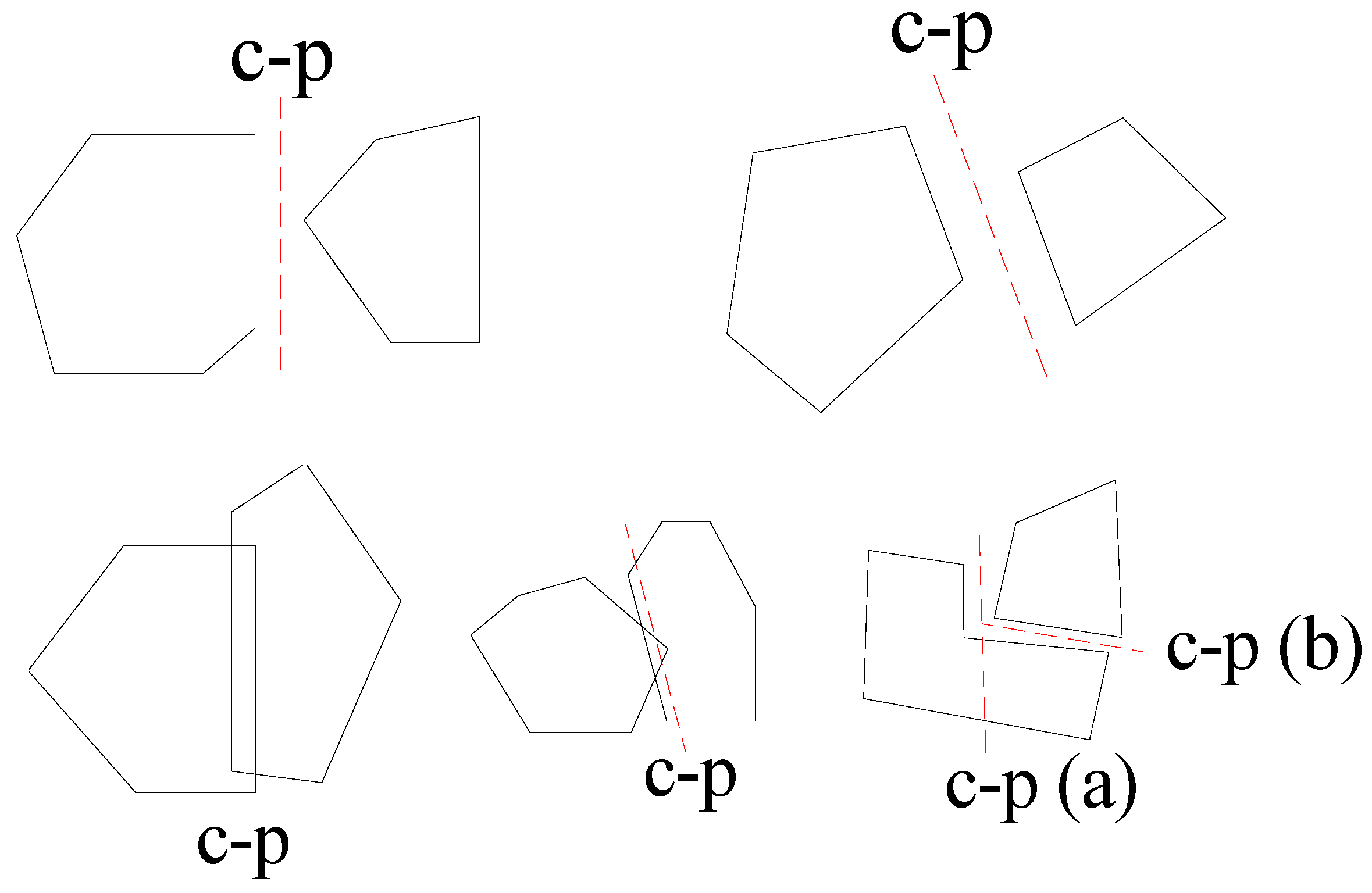
As shown in Figure 2, the two blocks modeled are fully bonded together, resisting tension and shear according to the Mohr–Coulomb law defined in Figure 1. Between the two blocks, there is a single contact (a single joint) corresponding to a surface. Cundall (1988) [30] introduced the common plane (c-p) method for contact identification (Figure 3), which was applied here (e.g., face-to-edge or vertex-to-face). This method involves first determining the plane that separates the space between the two polygons. Once the common plane is established, the contact between each particle and the plane is considered. Specifically, as the blocks (polygons in 2D and polyhedral in 3D) move closer, the plane is positioned halfway between them, at the maximum distance from both.

For deformable blocks, the triangular faces of the tetrahedral zones on the block’s surface contain internal surface nodes, each with three independent degrees of freedom. In this case, a sub-contact is generated for each node on the face. Two types of sub-contacts are defined: vertex-to-face and edge-to-edge. Edge-to-edge sub-contacts model both edge-to-edge contact between blocks and face-to-face or face-to-edge contacts at the intersection points of edges on the common plane If a block face contacts the c-p, it is discretized into sub-contacts.

The mesh size corresponds to the dimensions of a hexahedral zone within a six-sided polyhedron. Changing the mesh size alters the number of tetrahedral zones, which in turn changes the number of internal surface nodes, thus affecting the number of sub-contacts. Each sub-contact tracks the interface forces between blocks, as well as other conditions such as sliding and separation. When failure occurs at a sub-contact, whether in tension or shear, the tensile strength and cohesion are considered to be zero, reflecting the behavior of a ‘crack’ in a joint. A joint is considered fully broken when all sub-contacts within it have failed. Therefore, we consider the number of sub-contacts to correspond to the number of cracks that can exist.

The mesh size used was 25 mm, corresponding to the size of a hexahedral zone in a six-sided polyhedron (Figure 2). Block B1 was fully constrained in both displacement and rotation at its base. For the shear case, an incremental displacement was applied to all grid points in the Block B2 by assigning a constant velocity equal to 1 mm/s in the horizontal direction, while for the tensile case, the displacement was assigned in the vertical direction. For the blocks subjected to shear, the top face of the block B2 was fixed in the vertical direction to ensure that only the shear displacement is produced. A mix-mode tension/shear case was also conducted by using the same loading as the case of shear, but the top face of block B2 was left free in the vertical direction.

It is important to note that in the DEM, displacement is not directly imposed; instead, it is applied indirectly through the velocity. A given displacement ($u$) at a given time $\mathit{u}\left(t\right)={\mathit{u}}_0$ is obtained by prescribing a velocity $\mathit{v}\left(t\right)$ over a time ($t$) increment $\mathsf{\Delta }{t}_0$ such that ${\mathit{u}}_0={\int }_0^{\mathsf{\Delta }{t}_0}\mathit{v}\left(t\right)dt$. The velocity $\mathit{v}$ was kept small and constant to minimize dynamic effects during the application of the load.

3.2. Material Properties and Loading Conditions

The interface strength, defined by cohesion, friction, and tensile strength, was determined from the shear and direct tensile tests of Venzal et al. (2020) [31]. For the shear test, limestone blocks (10 cm × 10 cm × 10 cm) are initially subjected to a compressive load, resulting in normal stress on the mortar joint. Then, the central block is loaded with a vertical force, which induces shear at the interface. By varying the applied normal stress, the Mohr–Coulomb law $\tau =c+{\sigma }_{n}tan \phi$ is used to identify the cohesion ($c$) and friction angle ($\phi )$ once the shear limit is reached. For the tensile test, two assembled limestone blocks (10 cm × 10 cm × 7 cm) are glued together with epoxy resin inside a steel box, which is fixed to a testing machine to prevent rotation of the blocks during the direct tensile test.

The block was assumed to behave elastically with Young’s Modulus $E=10 \mathrm{G}\mathrm{P}\mathrm{a}$, Poisson ration $\mathrm{\nu }=0.2$, and density $D=2500 \mathrm{k}\mathrm{g}/{\mathrm{m}}^3$. An elastoplastic Mohr–Coulomb law with tension cut-off was used to represent the mortar joint with normal stiffness $k_n=20$ GPa/m, shear stiffness $k_s=7.8$ GPa/m, the friction angle $\phi =38°$, cohesive strength $C=0.25$ MPa, tensile strength $T=0.055$ MPa, and the dilatation angle ψ $=0$. The values of these parameters were based on the experimental tests of Venzal et al. (2020) [31] and later calibrated as in the study of Boukham et al. (2024) [32]. In the experiment, the blocks made of soft limestone sourced from the Frontenac quarry were bonded with a natural hydraulic lime mortar, commonly used in the restoration of historic building masonry. Lime-based mortar is softer than cement-based mortar, allowing it to accommodate smaller movements without cracking. The cracks in the joint induce wave propagations (with one or more cracks potentially appearing simultaneously), and an effort has been made to capture the vibrations on the surface of the blocks using virtual sensors in the model, which corresponds to an acoustic emission event (AE event corresponds to a resulting signal).

The use of surface velocity as a proxy for acoustic emission (AE) signals is based on the physical assumption that AE events result from rapid releases of elastic energy associated with micro-crack initiation and propagation, which generate stress waves traveling through the material. In this context, surface velocity provides a physically consistent representation of the dynamic response at the boundary of the specimen induced by internal damage processes. Unlike experimental AE measurements, which depend on sensor characteristics such as the frequency response, threshold settings, coupling conditions, and signal-processing procedures, the surface velocity obtained from the DEM model corresponds to a direct numerical output of the material’s dynamic behavior. This approach therefore offers a simplified representation of wave propagation phenomena associated with fracture evolution. However, it is acknowledged that this simplification may lead to differences compared to experimental AE signals, particularly in terms of the amplitude, frequency content, and event detection sensitivity. These limitations should be considered in the future when interpreting the correspondence between numerical results and experimental observations.

3.3. Numerical Implementation and Local Damping Study

Furthermore, the DEM employs an explicit time-stepping scheme to directly solve the equations of motion. 3DEC [33] is used to address two general types of mechanical problems: quasi-static and dynamic states. Damping is applied in both types of problems, though quasi-static problems typically require higher damping values. For static loading, a “local damping” method is used, where the damping force on a node is proportional to the magnitude of the unbalanced force [13,15]. The unbalanced force is a parameter to check when mechanical equilibrium (or the initiation of joint sliding or plastic deformation) is achieved in a static analysis. A model is considered to be in equilibrium when the net nodal force vector at each block centroid or grid point equals zero (or it is almost zero). The highest nodal force vector is commonly known as the “unbalanced” or “out-of-equilibrium” force. In the numerical analysis, the maximum unbalanced force will never precisely be equal to zero; however, the model is regarded as being in equilibrium when the maximum unbalanced force is relatively small compared to the forces typical of the problem. For deformable blocks, the equation of motion incorporates “local damping” as shown below:

$${\dot{u}}_i^{(t+∆t/2)}={\dot{u}}_i^{(t-∆t/2)}+\left\{{\displaystyle \sum }{F}_i^{\left(t\right)}-{\left(F_d\right)}_i\right\}{\displaystyle \frac{∆t}{m_n}}$$

(1)

where

$${\left(F_d\right)}_i=\alpha \left|{\displaystyle \sum }{F}_i^{\left(t\right)}\right| sgn\left({\dot{u}}_i^{(t-∆t/2)}\right)$$

(2)

$$sign\left(y\right)=\left\{\begin{array}{c}+1, if y>0\\ -1, if y<0\\ 0, if y=0\end{array}\right.$$

(3)

and $\alpha$ is a constant varied in the range of $0<\alpha <1$ (default of 0.8 in 3DEC for static loading), $m_n$ is the nodal mass, $F_i$ is the resultant of all external forces applied, and $F_d$ is the damping force obtained.

More precisely, the calculation in 3DEC is considered converged or in the static equilibrium state if the unbalanced force ratio is less than 1 × 10⁻⁴. The convergence speed of the model depends on both the applied velocity magnitude and the local damping used. In the study of Pulatsu et al. (2020) [26], the effect of loading speed on convergence was studied. They noted that a velocity of 10 mm/s gives significant oscillations in the wall behavior curve. A velocity between 1 mm/s and 0.1 mm/s gives curves with no fluctuations or noticeable differences observed. Therefore, in this study, a slow relative loading speed of 1 mm/s was used.

However, the impact of local damping on convergence is not addressed in the literature. The value of 0.8 is typically recommended for static calculations. In general, the higher damping speeds up convergence and reduces numerical oscillations, but it also decreases kinetic energy. However, in the case of acoustic emission, higher kinetic energy resulting from a broken joint makes it easier to capture the signal of elastic wave propagation. It is important to note that with local damping values between 0 and 1 ($0<\alpha <1)$, the structure will always reach a balanced state, but the convergence speed will vary depending on the damping value used. Therefore, it is crucial to study the effect of damping to achieve both fast convergence and a sufficiently clear vibration signal captured by an artificial sensor placed on the surface of the block. Concretely, the velocity (in y direction) of Block B1 was monitored at the sensor point (located at the center of the block’s face) (Figure 2b) during loading. In general, velocity in all three directions can be used but, in this study, only the y direction was examined.

3.4. Influence of Damping on Acoustic Emission Signal and Convergence

3.4.1. Effect of Damping on the Convergence Rate Following Joint Failure

Firstly, the shear loading case was here conducted. The effect of damping on the convergence rate following joint failure was investigated. The convergence criterion, based on an unbalanced force ratio limit of 1 × 10⁻⁴, was applied. The convergence rate was assessed by counting the total number of cycles required for the calculation to converge. Damping values were assumed to be ranging from 0.1 to 0.8. Next, the convergence rates of the other cases were compared with the case using a damping value equal to 0.8, which has been the only value utilized in the literature for quasi-static calculations. The ratio CNi/CN0.8 (cycle number of $\alpha =i$/Cyc number of $\alpha$ = 0.8) represents the ratio of the number of cycles (CN) with damping value i to the number of cycles with a damping value of 0.8.

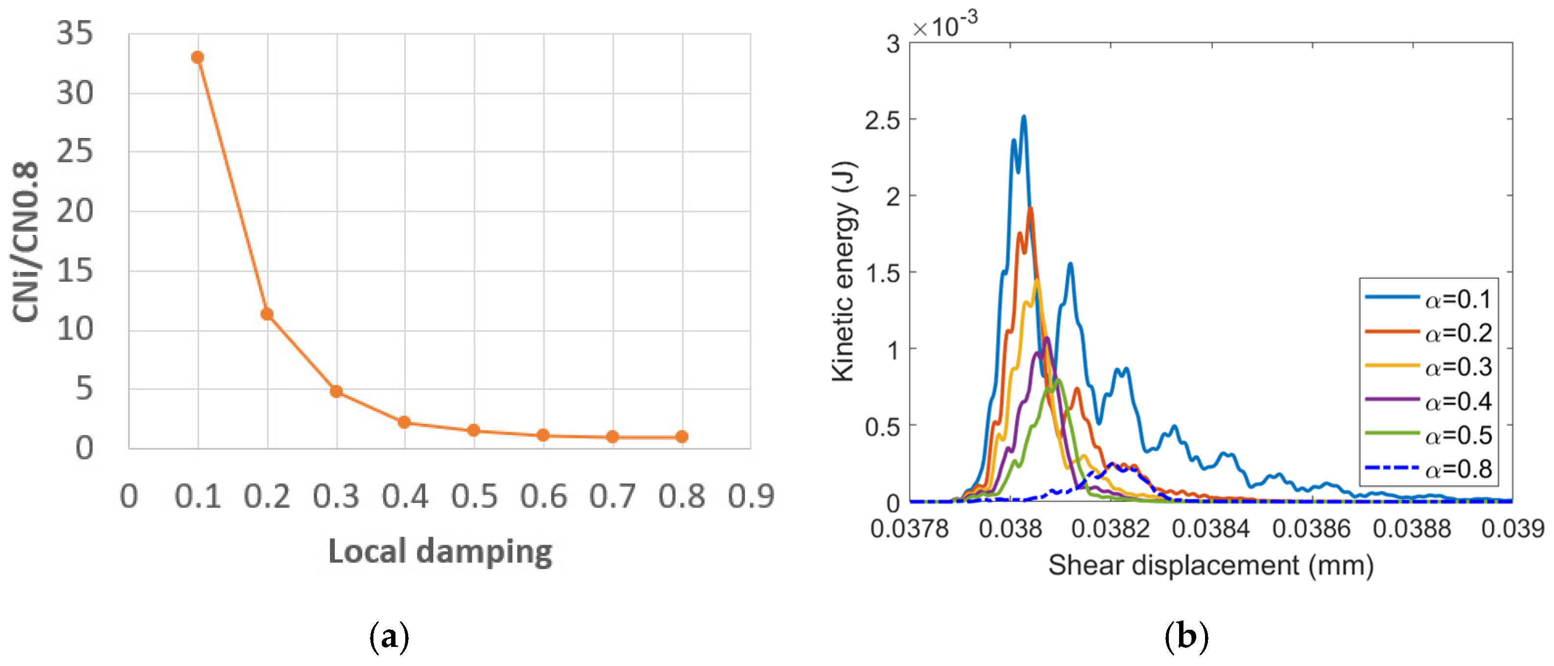
The results are presented in

Table 1. Effect of local damping on the cycle number.

$\mathbf{Local} \mathbf{Damping} \mathit{\alpha }$	0.1	0.2	0.3	0.4	0.5	0.6	0.7	0.8
Cycle number	625,453	215,043	89,548	42,009	27,649	20,625	17,870	18,938
$\mathit{C}\mathit{N}\mathit{i}/\mathit{C}\mathit{N}\mathbf{0.8}$	33.03	11.36	4.73	2.22	1.46	1.09	0.94	1.00

and Figure 4. For the case where $\alpha$ = 0.8, the calculation converges after 18,938 cycles following the joint failure. The damping values of 0.5, 0.6, and 0.7 result in cycle counts very similar to the case of $\alpha$ = 0.8. However, for damping values lower than 0.5, a significant increase in the number of cycles was observed. Specifically, damping values of 0.3 and 0.2 resulted in convergence speeds that are 5 and 11 times slower, respectively, compared to $\alpha$ = 0.8. The case of $\alpha$ = 0.1 showed an extremely slow convergence speed, taking 33 times longer than the case of $\alpha$ = 0.8. In numerical calculations, normally the cases in which the damping gave difficult convergence should be avoided.

3.4.2. Effect of Damping on the Load-Against-Displacement Curve

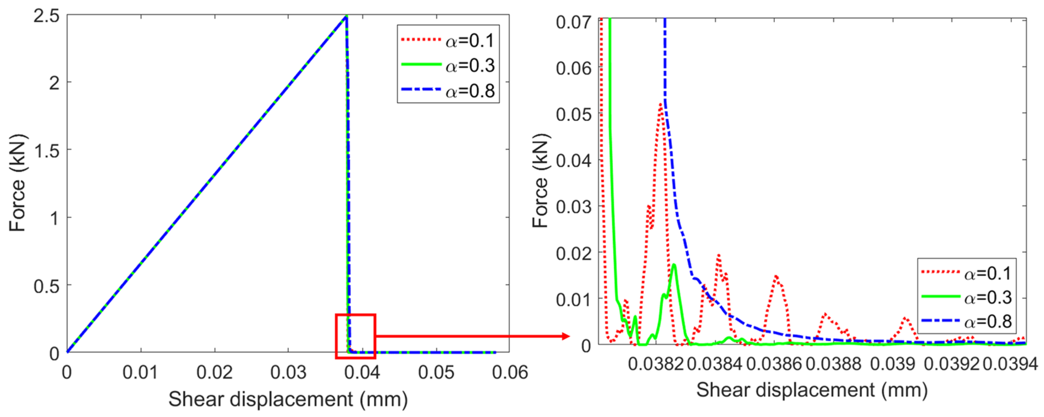
Figure 5 presents the effect of damping on the load-against-displacement curve of the specimen. From Figure 4, damping does not affect the ultimate load or the post-peak response (drop after ultimate load). However, when zooming in at the end of the drop, it was found that for the damping case $\alpha$ = 0.8, the curve is smooth, whereas for lower damping values, particularly for the 0.1 case, oscillations in the response were observed.

3.4.3. Effect of Damping on the Kinetic Energy and Velocity Signal

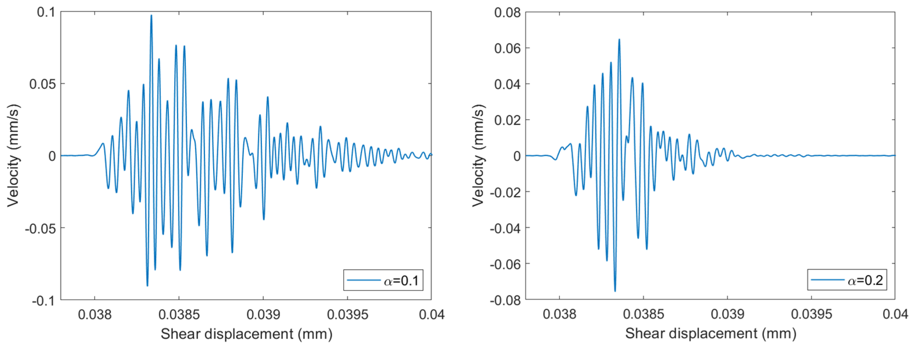
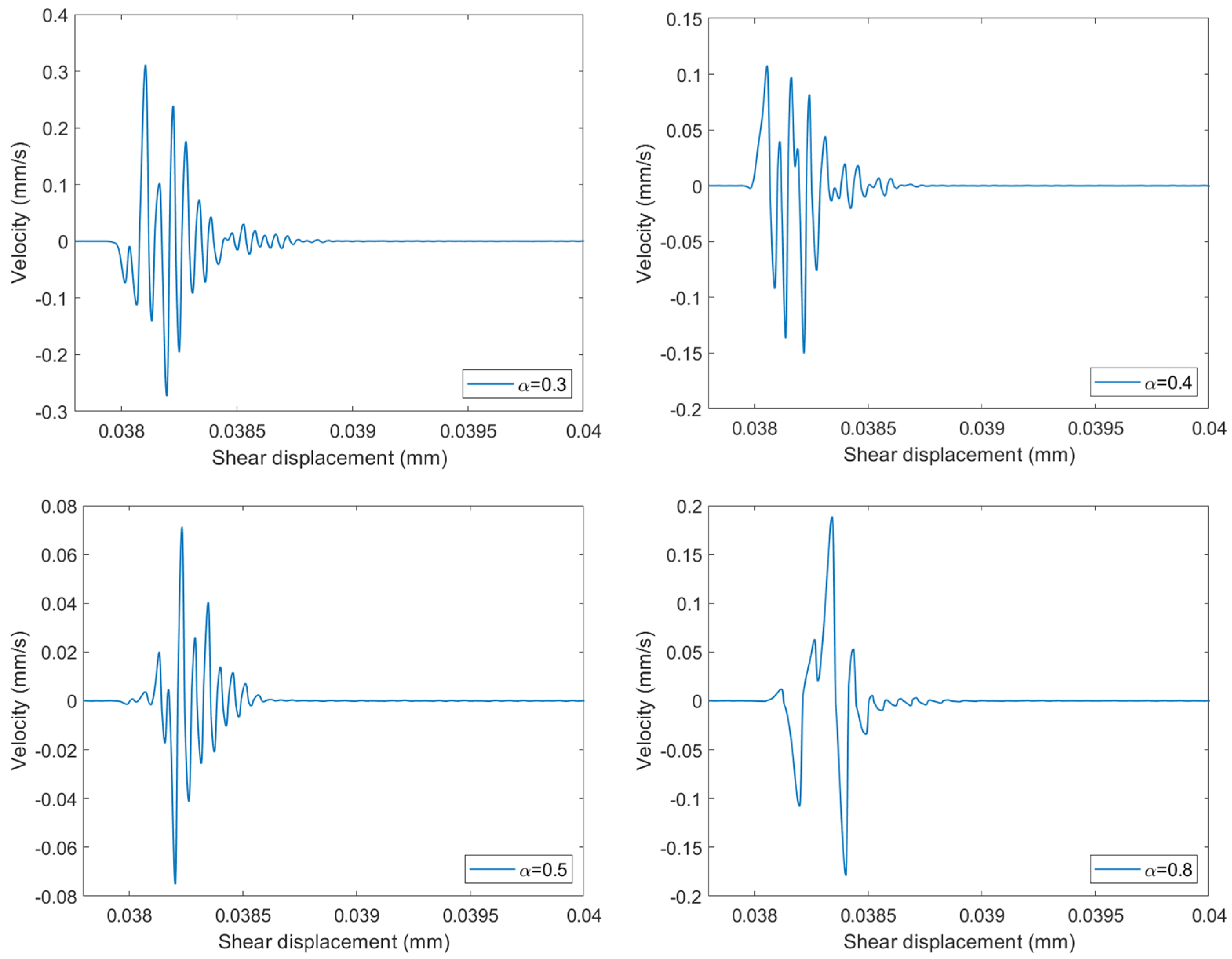
The effect of damping on the kinetic energy and the velocity signal measured at the monitoring point on the block in the numerical model is shown in Figure 4b and Figure 6. It is observed that as damping increases, the generated kinetic energy decreases. Additionally, the signal captured by measuring the velocity on the block surface after joint failure becomes less distinct, as indicated by fewer peaks in the signal.

Therefore, selecting the appropriate damping value for quasi-static calculations to simulate the AE remains a challenging task. In particular, the choice of the damping must balance fast convergence with minimal noise in the behavior curve, while at the same time ensuring a measured velocity signal after cracking with as many peaks as possible. To capture AE effectively, the case that provides a clearer velocity signal (with more peaks) corresponds to a lower damping value. However, based on the results obtained, damping values of 0.1 and 0.2 are not recommended, as they lead to excessively slow convergence (33 times and 11 times slower, respectively), despite producing a good velocity signal. Therefore, initially, a damping value of 0.3 was used.

3.4.4. Evolution of Total Energy Released and Strain Energy Stored in the Joint

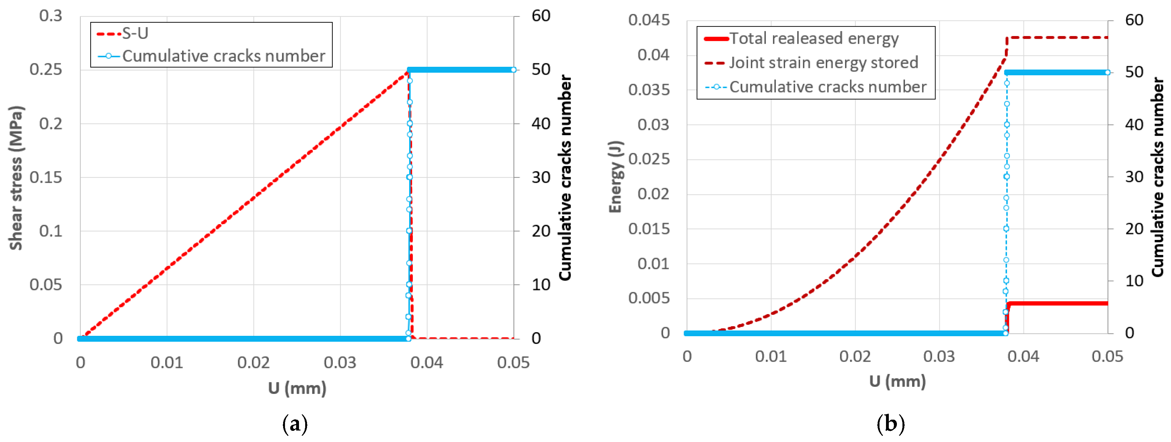
For the direct shear test, Figure 7a shows the shear stress and the cumulative number of cracks (representing cumulative AE events) as a function of shear displacement. It should be noted that the number of cracks in the numerical model corresponds to the number of “sub-contacts” that occur during the failure of a broken joint. In the case of numerically simulating two blocks in shear, there are multiple “sub-contacts” at the zero-thickness interface between the two blocks. A “sub-contact” is defined as the contact between the meshes of each surface of the block. The definition of a sub-contact in the DEM is based on the concept of the “common plane”. The number of sub-contacts depends on the mesh size of the contact established. In this case, 50 sub-contacts were detected in the model, meaning that the maximum number of cracks that can be formed is in 50 locations. The shear stress–displacement curve was found to be quasi-linear until the shear strength of 0.25 MPa was reached, after which a sudden drop in the load to zero was observed. This drop coincides with a rapid increase in the number of cracks forming in the joint, ultimately leading to complete failure of the joint.

The evolution of the total released energy and the strain energy stored in the joint is shown in Figure 7b. The strain energy in the joint consists of four components: (i) elastic deformation in shear; (ii) compression; (iii) tension, and (iv) energy dissipated during sliding. The energy dissipated during sliding ($U_{jf}$) is established when the current shear force ($f_s$) at a contact is greater than or equal to shear stress maximal ($f_{s max}$) at which the Coulomb slip condition is met ($f_{s max}=f_{n}tan \phi +c$). This energy is calculated by $U_{jf}={\displaystyle \frac{1}{2}}\left(f_s+f_s^{\mathrm{\prime }}\right)u_s$, where $f_s^{\mathrm{\prime }}$ is previous shear forces at a contact and $u_s$ is incremental shear displacements at the contact over the current timestep. The strain energy reaches its maximum when the load reaches its ultimate limit. A similar observation was made in the study by Zhang et al. (2021) [34], albeit for a coal specimen under compressive loading. During cracking, a substantial portion of the energy is released, which accounts for the generation.

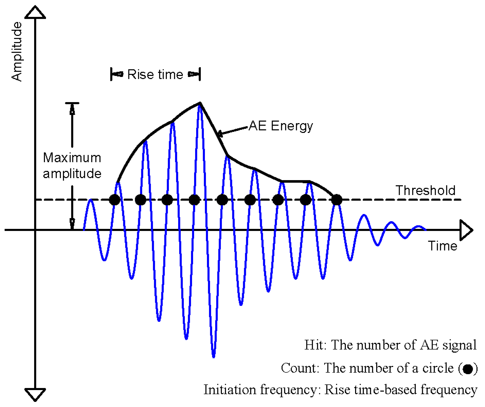
The AE energy is calculated by integrating the AE signal over time, above a specified threshold value (Figure 8). In the numerical simulation, the PZT sensor was not modeled. Instead, the AE phenomenon was captured through elastic waves, represented by the velocity measured at the surface of the block. While the AE signal in the experiment is captured by a PZT sensor, in the numerical simulation, the AE signal is measured by the velocity at the surface of the block. To enable a comparison between the two types of signals, only the ‘normalized’ results were used. The method of using velocity as an AE signal has already been applied in the discrete element method for materials like concrete. A similar study comparing normalized cumulative AE energy using the signal captured by a PZT sensor and the signal measured by velocity in numerical simulation can be found in Rucka et al. (2023) [22]. The number of peaks detected in the velocity signal can be used to count the cumulative number of AE hits, which is one of the key parameters of acoustic emission.

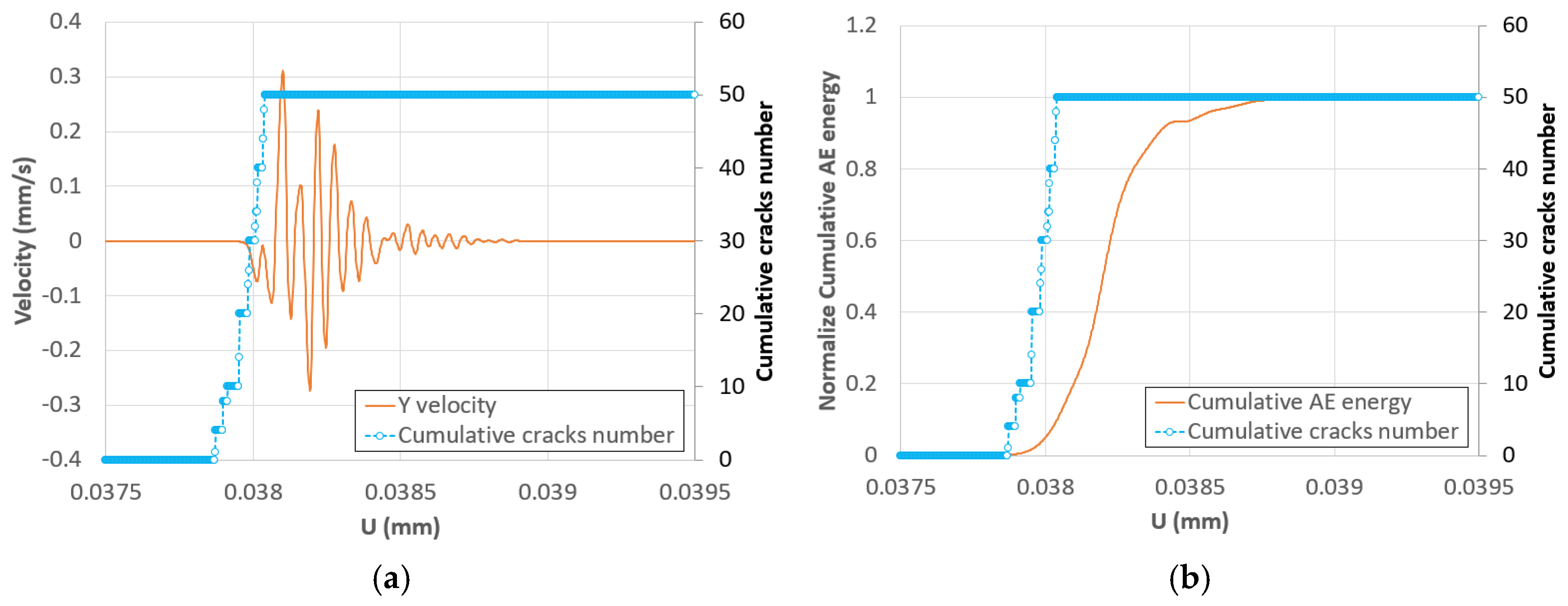
In this simulation, a velocity signal with a sudden increase in amplitude was observed on the block surface once cracking in the joint was initiated (Figure 9a). In acoustic emission, the cumulative AE energy is an indicator for assessing cracks. Therefore, the cumulative AE energy is calculated here and compared with the cumulative number of cracks. The cumulative AE energy is calculated based on vibration measurements on the block below. The cumulative AE energy can be calculated over shear displacement instead of time because the applied displacement is linearly proportional to time (imposed displacement). The cumulative AE energy increases rapidly as cracking propagates (see Figure 9b). Also, it was observed that there is a discrepancy between the cumulative crack number and the cumulative AE energy. When cracking occurs, it takes time for the waves to be transmitted and captured by the sensor point on the block. Once the velocity capture is delayed relative to the moment the cracks appear, the energy calculated is also shifted. It should be noted that velocity and cumulative AE energy can only detect crack initiation, as more than 10 cumulative cracks were detected in the joint (out of 50 total cracks by the end).

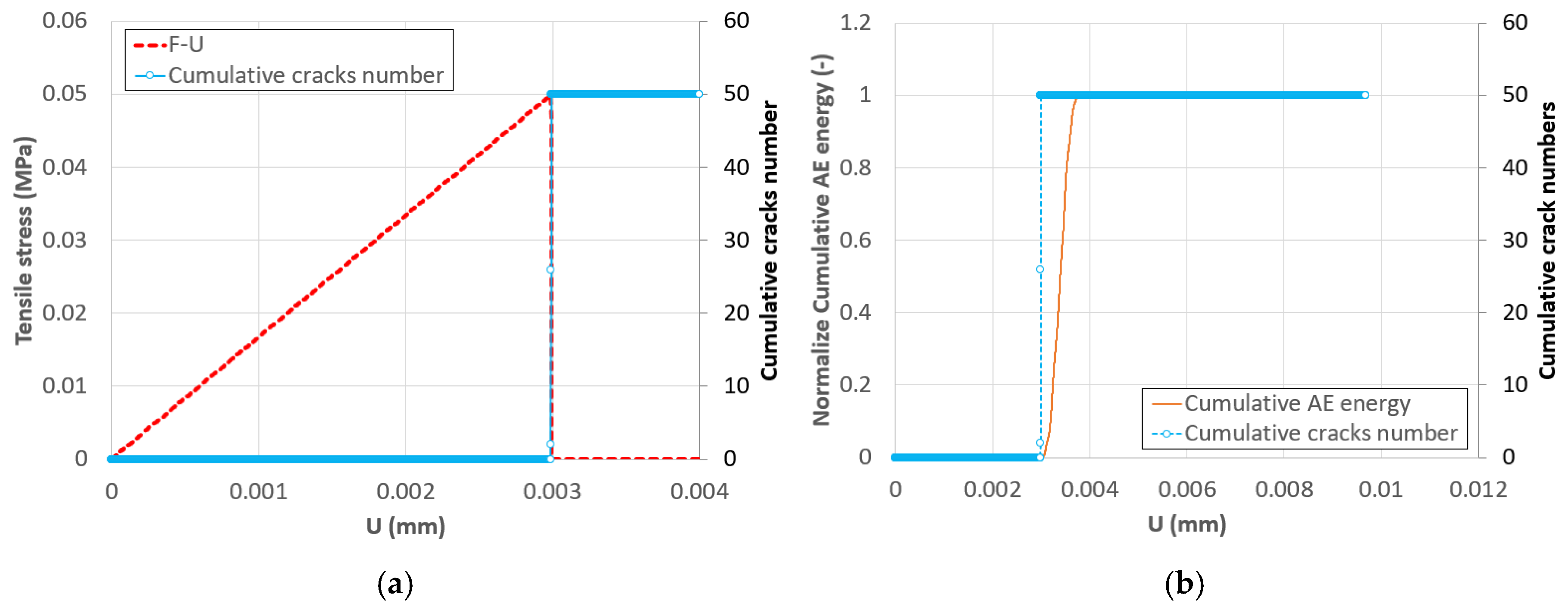
In the tension loading case, the load/deflection curve exhibits linear behavior up to the ultimate load of 0.05 MPa, after which there is a rapid decline in tensile strength to zero, corresponding to the broken bonds in the contacts. This is captured by the increase in the cumulative crack number (Figure 10a). The monitoring of velocity and energy can detect the initiation of rupture as soon as the first crack appears.

3.4.5. Comparisons with Recent Studies

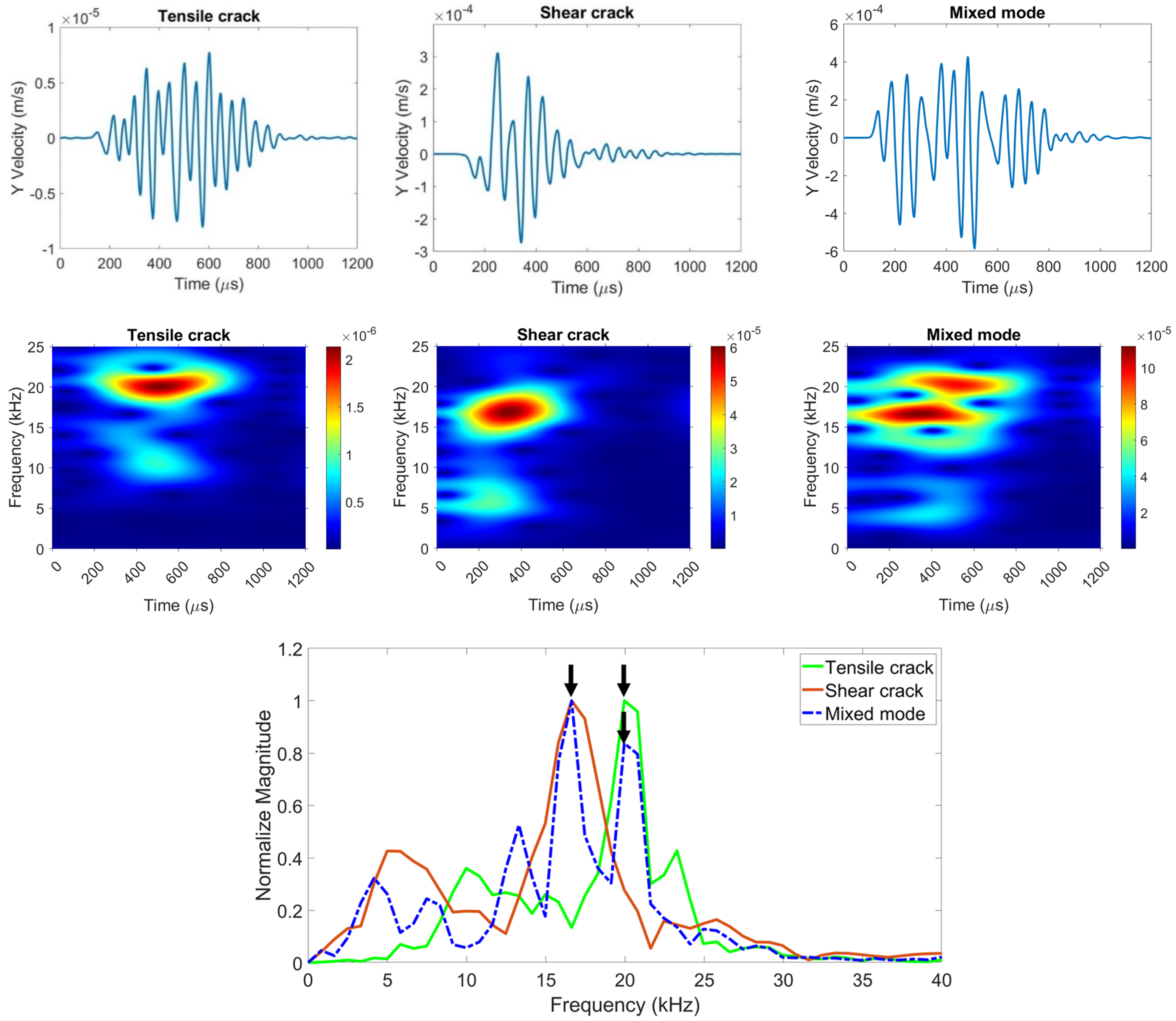
Recent studies [34,35,36,37,38] have shown that frequency analysis of each AE hit can provide additional information on cracking modes. More specifically, the results indicate that the same AE signal can contain signatures of both shear and tension cracks, with shear cracks corresponding to lower frequency ranges and tension cracks to higher frequency ranges. Mandal et al. (2024) [35] made the measurements of the acoustic emission on a reinforced concrete T-beam under bending. The results showed that shear bands are identified as low-frequency bands (below approximately 200 kHz) that exhibit higher values during shear cracking events. In contrast, tension bands are high-frequency bands (above 250 kHz) that show increased values during tension cracking events. In this study, the frequency–time images and the Fourier transforms of signals obtained from a velocity signal for the three cases is presented: (i) tensile, (ii) shear cracking, and (iii) mixed tension and shear modes. The velocity signal (in the y-direction) in the three cases is consistently measured at the same point at the center of the block’s base. Additionally, the signal is measured when the crack is detected in the joint. The results show that shear cracks produce a frequency of approximately 17 kHz (Figure 11), while tensile cracks produce a frequency of around 20 kHz (Figure 11). This further confirms that tensile cracks generate higher frequencies than shear cracks. The case of the mixed mode tension/shear loading finds these two frequencies of two modes well. These results confirmed that the frequency-based index can be used to differentiate cracking modes based on the monitored AE signal.

3.4.6. Sensitivity of the Mesh Size

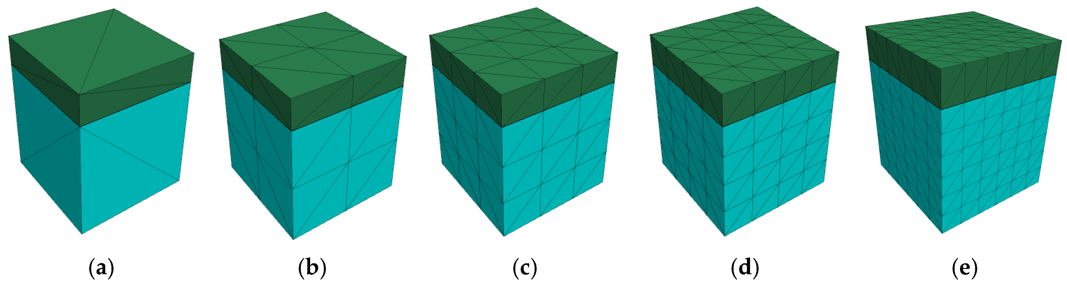
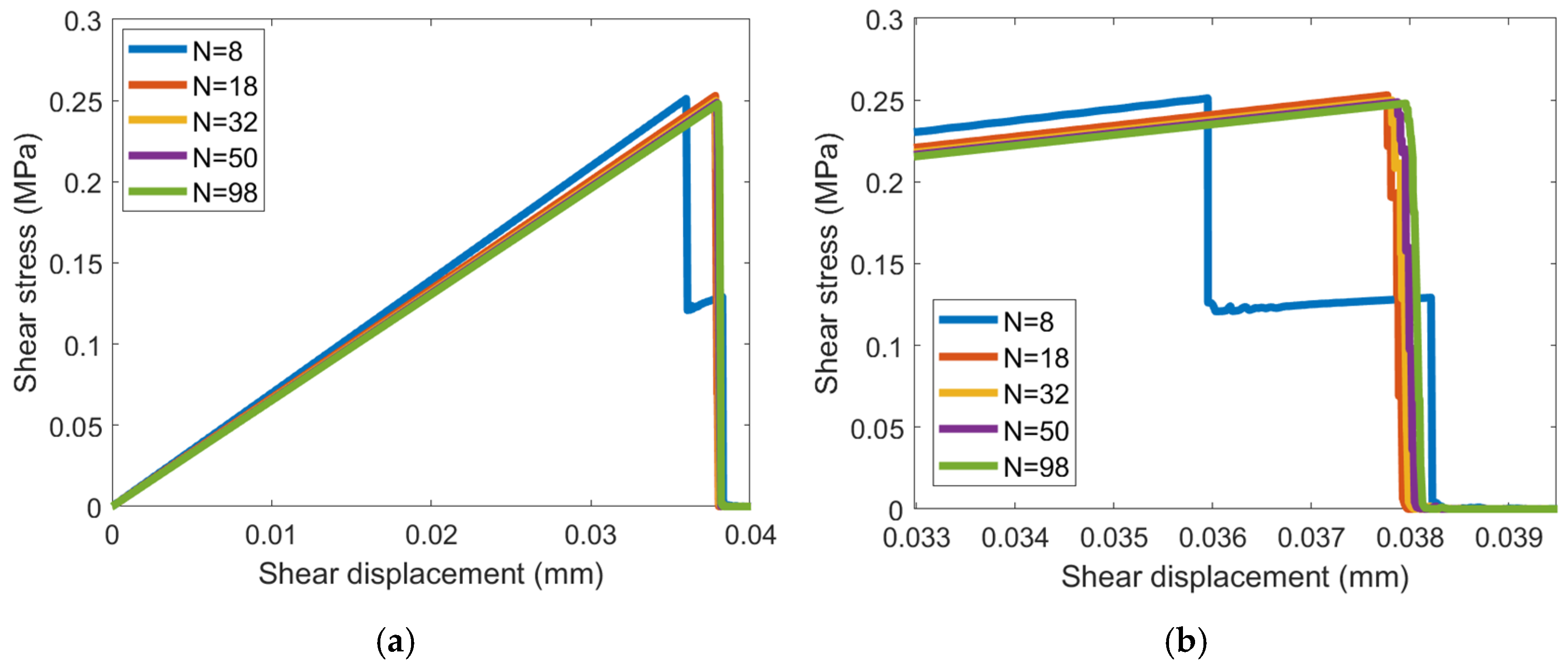
Also, the mesh size effect was investigated by varying the number of elements on each side of the block with 1 × 1, 2 × 2, 3 × 3, 4 × 4, and 6 × 6, corresponding to 8, 18, 32, 50, and 98 sub-contacts in the joint, respectively (Figure 12). The joint behavior was found to be influenced by the number of sub-contacts generated. First, the mesh effect was assessed by analyzing the shear stress–shear displacement curve under shear loading (Figure 13). Mesh convergence was observed when the number of sub-contacts N was equal to 18. Additionally, for the finer mesh, there was a slight delay in the moment when the load reached its ultimate strength.

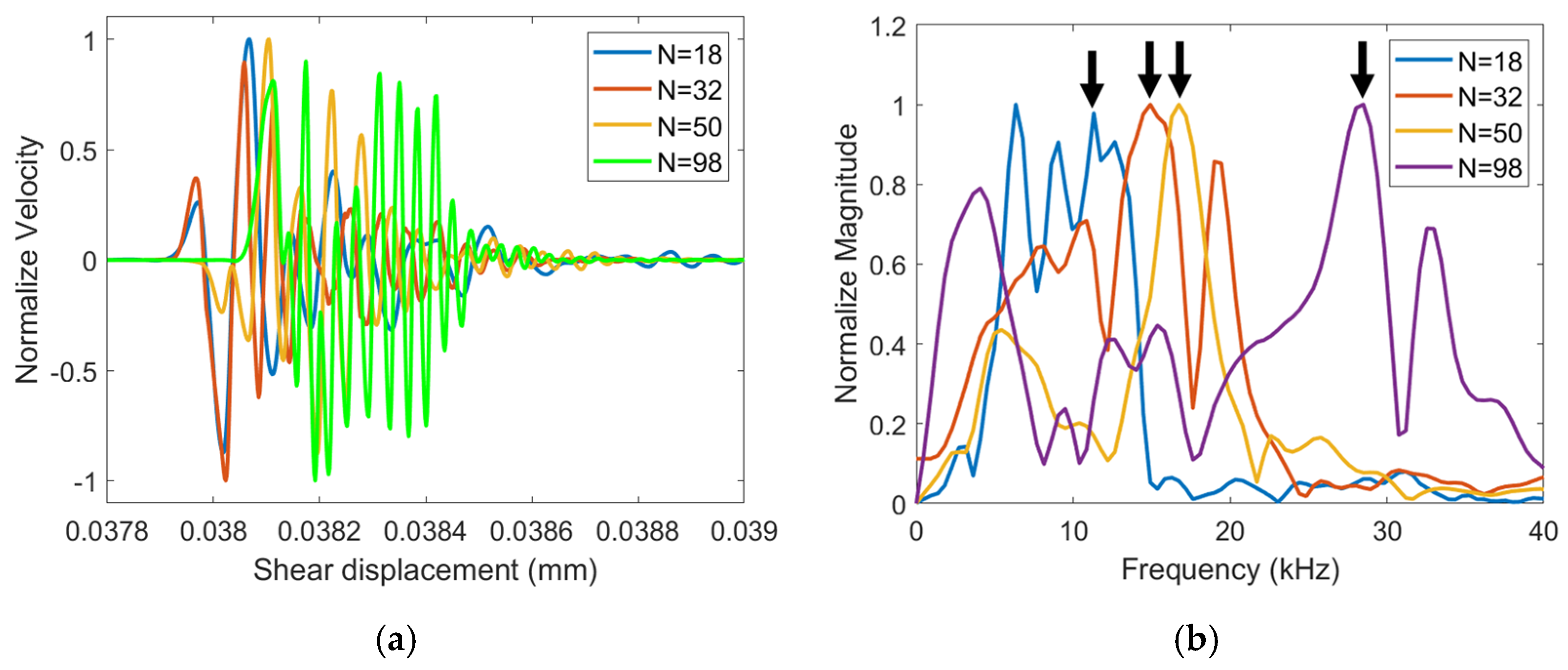
Then, the velocity at the center point of the bottom block surface was measured and compared across different mesh sizes. The velocity signals differ between the various mesh sizes. A Fourier transform (FFT) of velocity signals was applied. The frequencies obtained were 11.3 kHz, 14.9 kHz, 16.7 kHz, and 28.5 kHz for meshes with sub-contact numbers of N = 18, N = 32, N = 50, and N = 98, respectively (Figure 14). Additionally, as the mesh was refined, the obtained frequency increased. Therefore, it was concluded that mesh convergence cannot be achieved based on the velocity signal.

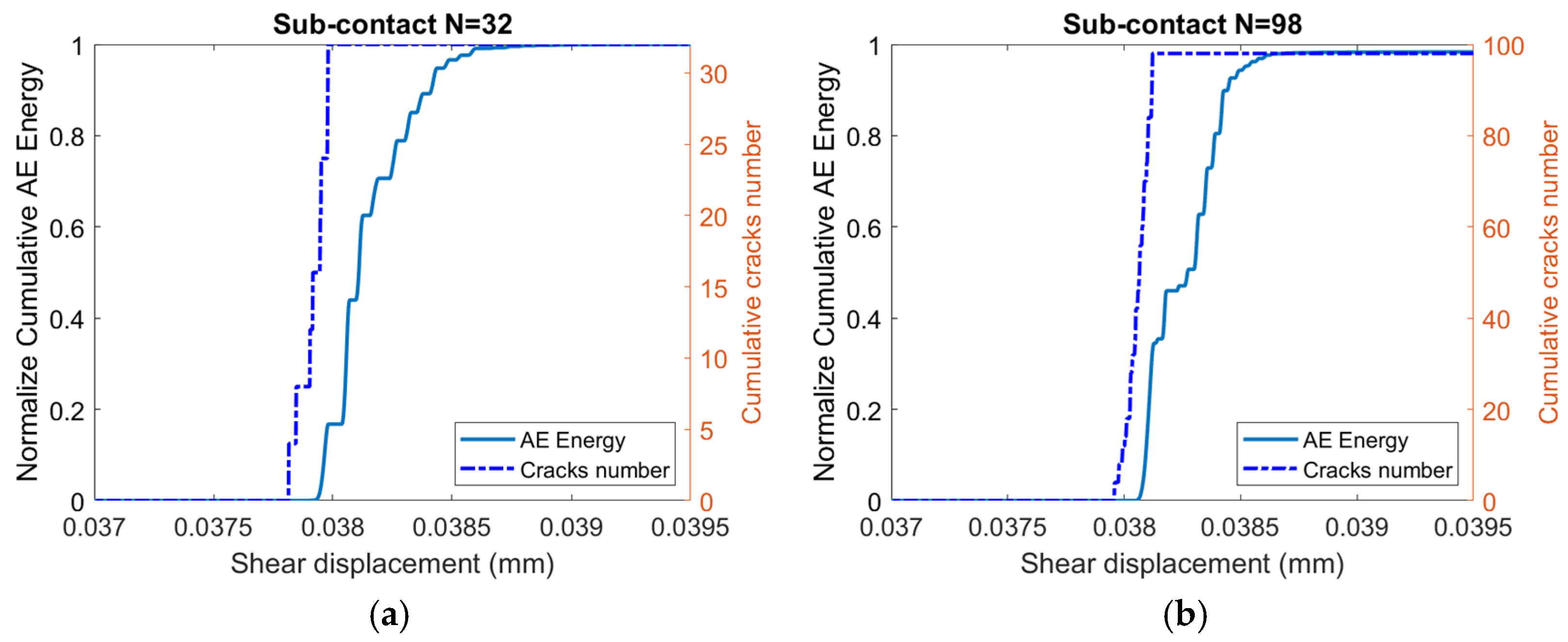
The key question here is whether, despite the differences in velocity signals for different meshes, analyzing these signals can still allow us to detect cracks in the model and whether a frequency analysis can identify the type of cracks. Therefore, the cases of N equal to 32 and N equal to 98 were analyzed. It was observed that the cumulative energy of the acoustic emission increases with the cumulative number of cracks (Figure 15). This tendency is similar to the case of the reference mesh N equal to 50, which was discussed earlier.

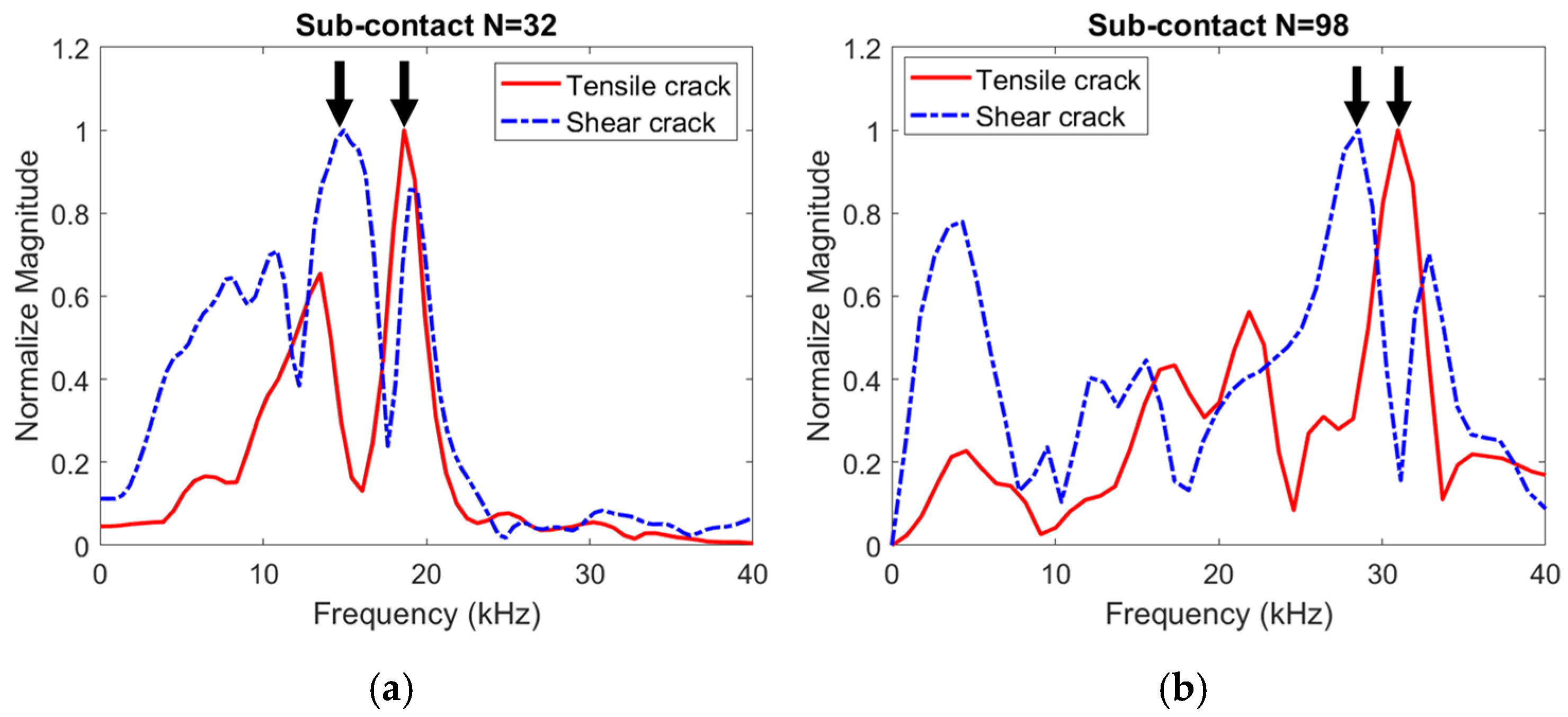
To verify whether frequency analysis can identify the different types of cracks, a Fourier transform (FFT) was applied to the velocity signal measured under shear and tension loading. It was observed that, although the frequencies obtained differ between the two mesh sizes, the frequency in the tension case was higher than in the shear case (Figure 16). For the mesh with a sub-contact number N equal to 32, the frequencies were 14.9 kHz for shear and 18.6 kHz for tension. For the mesh with a sub-contact number of N equal to 98, the frequencies were 28.5 kHz for shear and 31.0 kHz for tension. A change of approximately 3.5 kHz was observed between the shear and tension modes in both mesh size cases.

Therefore, mesh convergence can be achieved based on the overall behavior curve of the structure (e.g., force/displacement curve). However, the measured velocity signal cannot be used to achieve the mesh convergence. On the other hand, once mesh convergence is reached by using the behavior curve, the velocity signal can be utilized to simulate acoustic emission, despite differences in the velocity signals between different mesh sizes.

The results obtained in this section demonstrate the effectiveness of using the DEM to simulate the AE of a masonry joint subjected to both tension and shear. In the following section, the same method is applied to monitor the rupture of a masonry wall subjected to monotonic in-plane loading.

4. Acoustic Emission Using DEM to Simulate the Masonry Wall Under In-Plane Loading

4.1. In-Plane Loading Masonry Wall

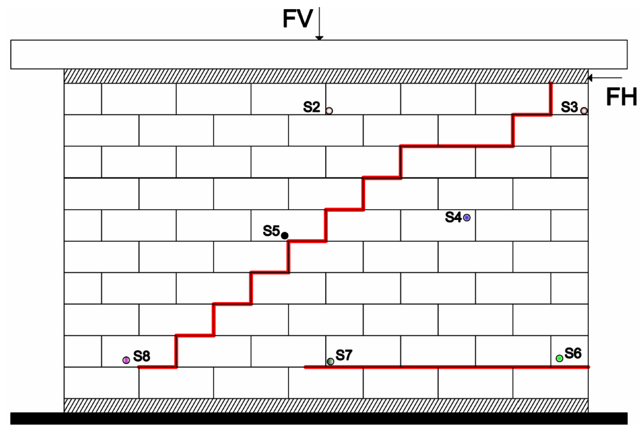
The experimental test of a masonry wall subjected to shear loading is based on the study by Peng et al. [9,39]. In this study, a wall with dimensions equal to 1.835 m × 1.15 m × 0.15 m and 11 brick lines was constructed and tested under shear loading (Figure 17). The wall was fixed at the bottom and initially subjected to a pre-compression of 0.4 MPa. This pre-compression was maintained constant, while a static horizontal load was applied to the top of the wall until failure. The failure mechanism in this type of test depends on both the wall’s geometry ratio (H/L, height/length) and the magnitude of the applied pre-compression. The pre-compression value of 0.4 MPa results in a mixed-mode failure, characterized by bending towards the base of the wall and shear along the diagonal line. Since the pre-compression is not excessively high, failure occurs mainly in the joints rather than in the bricks themselves. Therefore, this test is primarily used to evaluate the failure mechanism of the joints in the masonry wall.

To assess the damage using AE, six AE sensors were placed at different positions on the upstream face of the wall (Figure 17). For the subsequent numerical calculations, only the experimental measurements from the S8 sensor will be compared with the numerical results. The first crack detected in the wall is located near sensor S6, likely due to bending. Sensor S8, positioned at the farthest point from this crack, was selected to assess the model’s ability to monitor crack formation even when it is distant from the source.

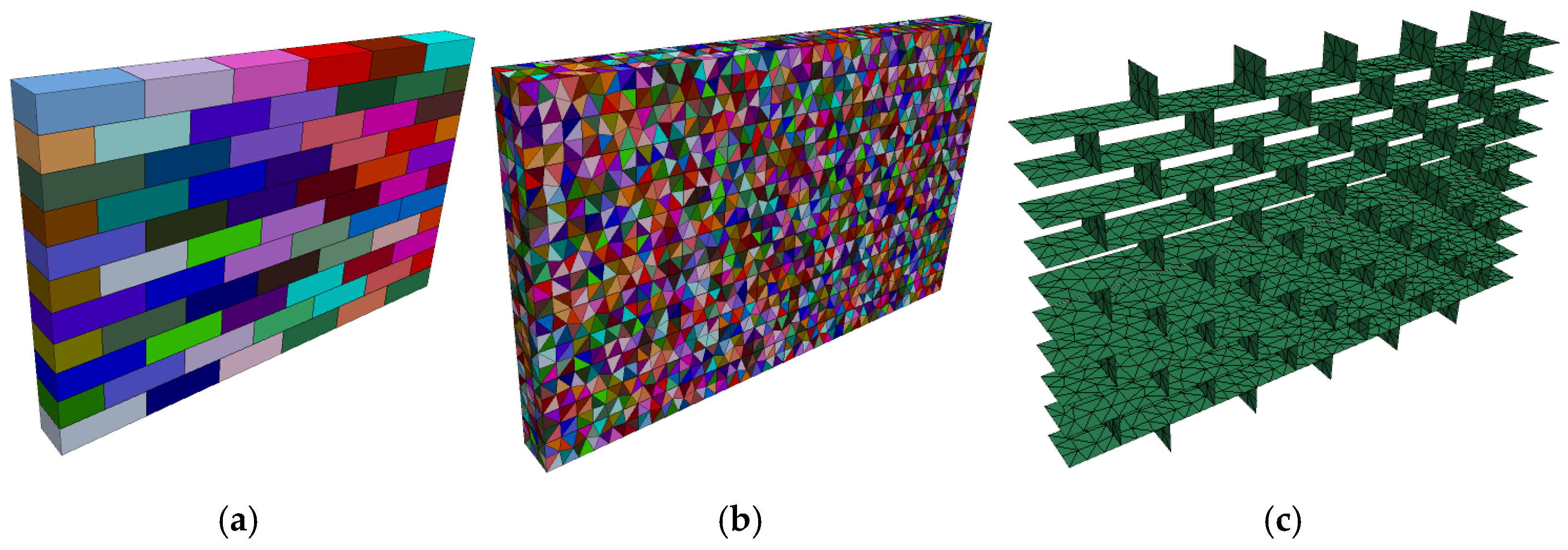
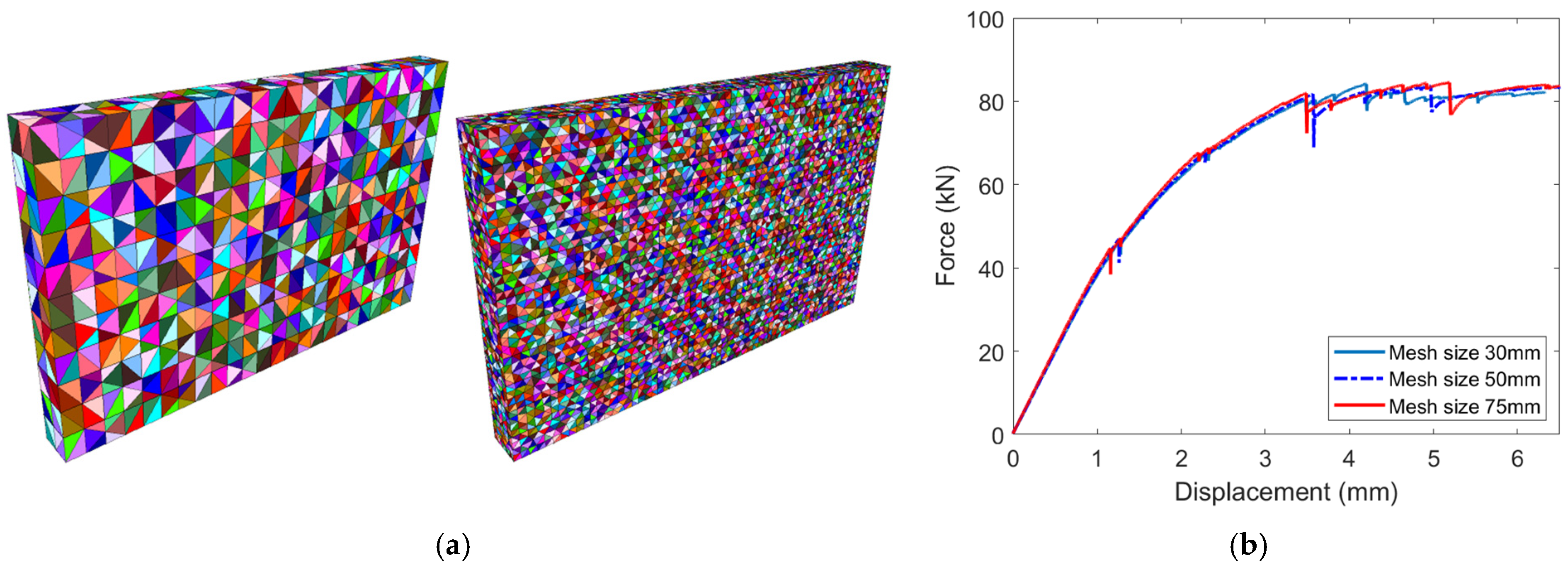
The masonry wall was modeled using the Discrete/Distinct Element Method (DEM) software 3DEC developed by Itasca (version 4.1). The wall in the numerical model consisted of 61 bricks, each with dimensions equal to 0.305 m × 0.106 m × 0.15 m, and 10 half-bricks, each with dimensions of 0.1525 m × 0.106 m × 0.15 m, resulting in a final wall size of the wall equal to 1.83 m × 1.166 m × 0.15 m (Figure 18a). Each deformable block was discretized into tetrahedral zones within a convex polyhedron of an arbitrary shape, with an edge length of 50 mm. A mesh convergence study has been carried out, and a mesh size equal to 50 mm was found to be appropriate. This discretization generated a total of 16,419 tetrahedral zones (Figure 18b) in the masonry wall, corresponding to 5992 sub-contacts between the blocks (Figure 18c).

A similar masonry wall was modeled in the study by Boukham et al. (2024) [32] using a Non-Smooth Contact Dynamic (NSCD) model. The joint characteristics from their study were also utilized in the calculations herein. Additionally, for the development of the computational model, it was assumed that the blocks remained in an elastic state, while only the joints exhibited elastoplastic behavior. The blocks were assumed to be elastic, with material properties of E = 10 GPa, ν = 0.2, and D = 2500 kg/m³. An elastoplastic Mohr–Coulomb law with a tension cut-off was used for the joints, with parameters ${\mathrm{k}}_{\mathrm{n}}=20 \mathrm{G}\mathrm{P}\mathrm{a}/\mathrm{m}$, ${\mathrm{k}}_{\mathrm{s}}=7.8 \mathrm{G}\mathrm{P}\mathrm{a}/\mathrm{m}$, the friction angle $\phi =46.5°$, cohesion $\mathrm{C}=0.27 \mathrm{M}\mathrm{P}\mathrm{a}$, tension $\mathrm{T}=0.05 \mathrm{M}\mathrm{P}\mathrm{a},$ and the dilatation angle $\mathsf{\varphi }=0°$. In the study by Boukham et al. (2024) [32], a more complex behavior constitutive law for joints under tension and shear, incorporating softening based on fracture energy, was used. In contrast, in this study, a simplified joint behavior law, as described in the previous section was utilized.

4.2. Numerical Results

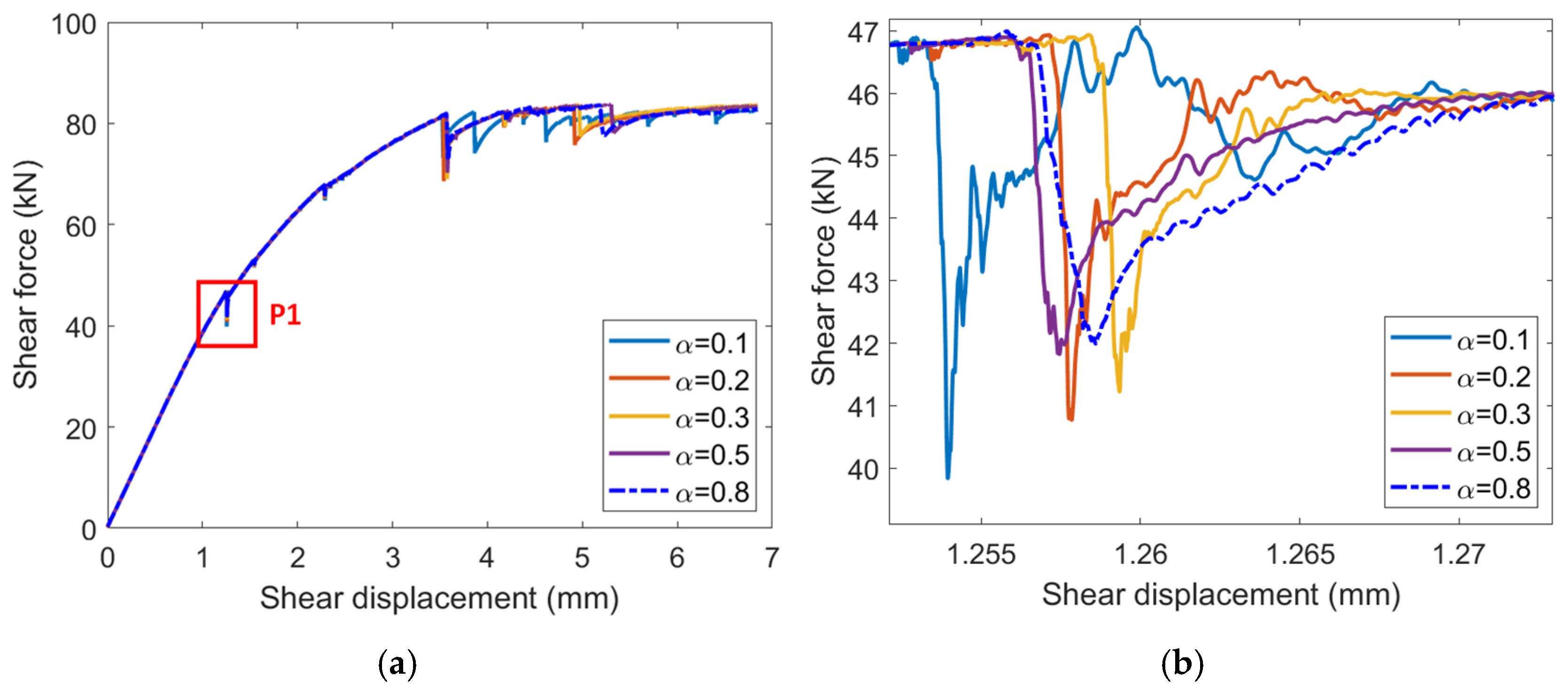
The effect of local damping was first examined based on the load/deflection curve of the structure’s behavior, with damping values ranging from 0.1 to 0.8. Figure 19 shows the force versus displacement curves for the different damping values used in this study. The curves are quite similar, showing the same general trend, with the same failure load observed across all cases. However, when zooming in on the initial load drop (point P1), it is evident that lower damping induced a deeper drop in loading. As discussed in the previous section, initially, a damping ratio equal to 0.3 was used to model AE. If the AE phenomenon cannot be captured, further reduction in damping can be considered.

In the numerical model, deformable blocks are made up of tetrahedral finite-difference zones, where mechanical changes (e.g., stress/strain) are calculated within each zone. As a result, the meshing algorithm generates elements that are random and cannot be controlled by the user. The only way to verify the suitability of the mesh is to calibrate the model using experimental results and check for mesh size convergence. The mesh convergence was verified herein through the load versus displacement curve of the wall, using three mesh densities: 30 mm, 50 mm, and 75 mm (Figure 18b and Figure 20a). The stiffness of the curve before the sudden drop at 3.57 mm was very similar for the 30 mm and 50 mm mesh sizes (Figure 20b). The larger 75 mm mesh showed a higher stiffness compared to these two cases. Based on this, the mesh converged can be considered at a size of 50 mm.

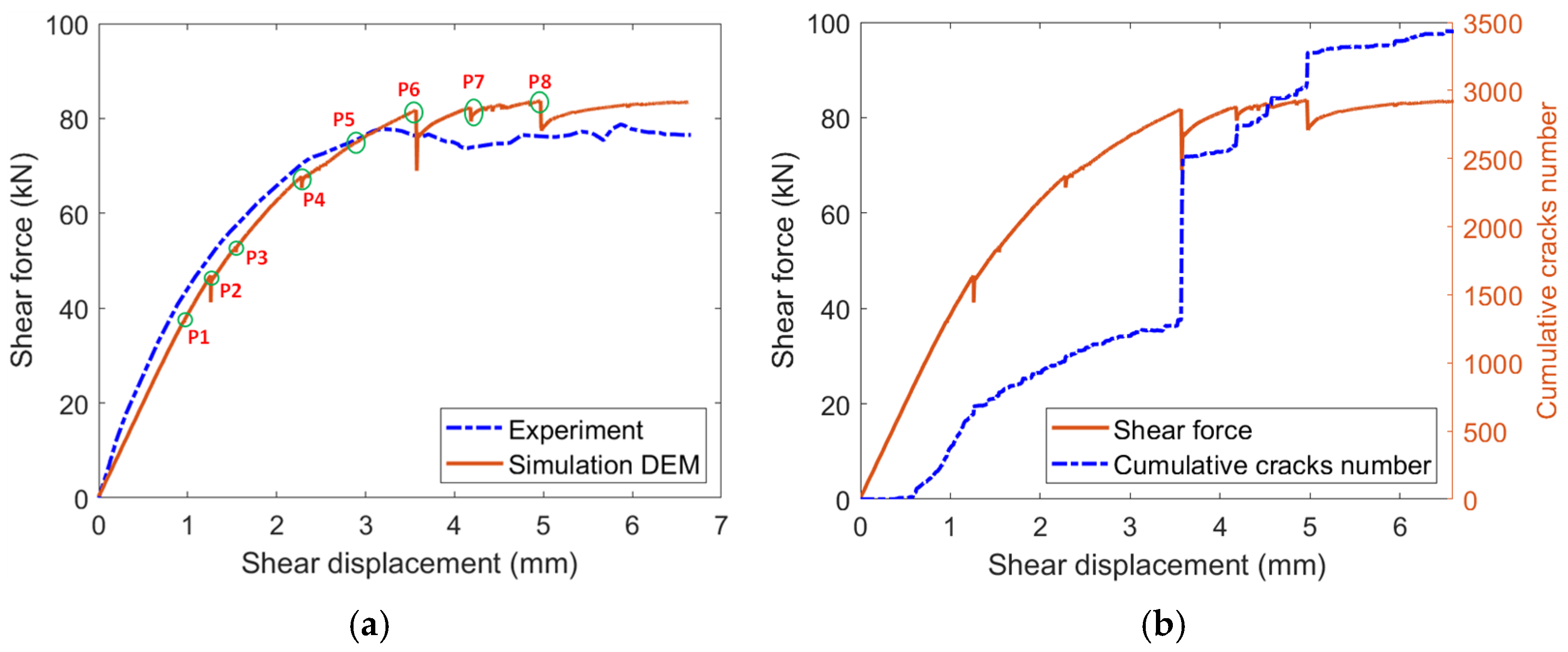
To evaluate the relevance of the numerical model, the shear force versus shear displacement curve was first compared between the experimental and numerical results; see Figure 21a. From Figure 19a, the numerical curve closely matches the experimental curve from the linear elastic phase to failure. In the numerical model, only the failure of the brick interface was used, which is normally enough because in the experimental test, only the cracks in joints were observed. However, the stiffness in the elastic phase of the numerical model was slightly lower than that observed in the experiment. The numerical ultimate load was 83.67 kN, which deviates by only 6% from the experimental load (${\mathrm{F}}_{exp}=78.75 \mathrm{k}\mathrm{N}$). Additionally, the numerical ultimate load occurs slightly later, at point P8 ($\mathrm{U}=4.96 \mathrm{m}\mathrm{m}$), compared to point P6 ($\mathrm{U}=3.57 \mathrm{m}\mathrm{m}$) in the experiment, where a sudden drop was observed. After reaching the ultimate load, both the experimental and numerical results showed a plateau in the load.

Although the numerical results show generally good agreement with the experimental observations, some discrepancies are observed in the elastic stiffness and peak load response. The simulated stiffness is lower than the experimental response, which can be attributed to several simplifying assumptions adopted in the DEM model. The blocks are assumed to behave purely elastically throughout the simulations, whereas local cracking or damage may occur within certain blocks in the experimental specimens under higher loading levels. In addition, the mortar layer between blocks is simplified as a zero-thickness joint interface. In the real structure, the mortar possesses a finite thickness and contributes to the deformability and load transfer behavior of the assembly. These simplifications may affect both the initial stiffness and the evolution of failure.

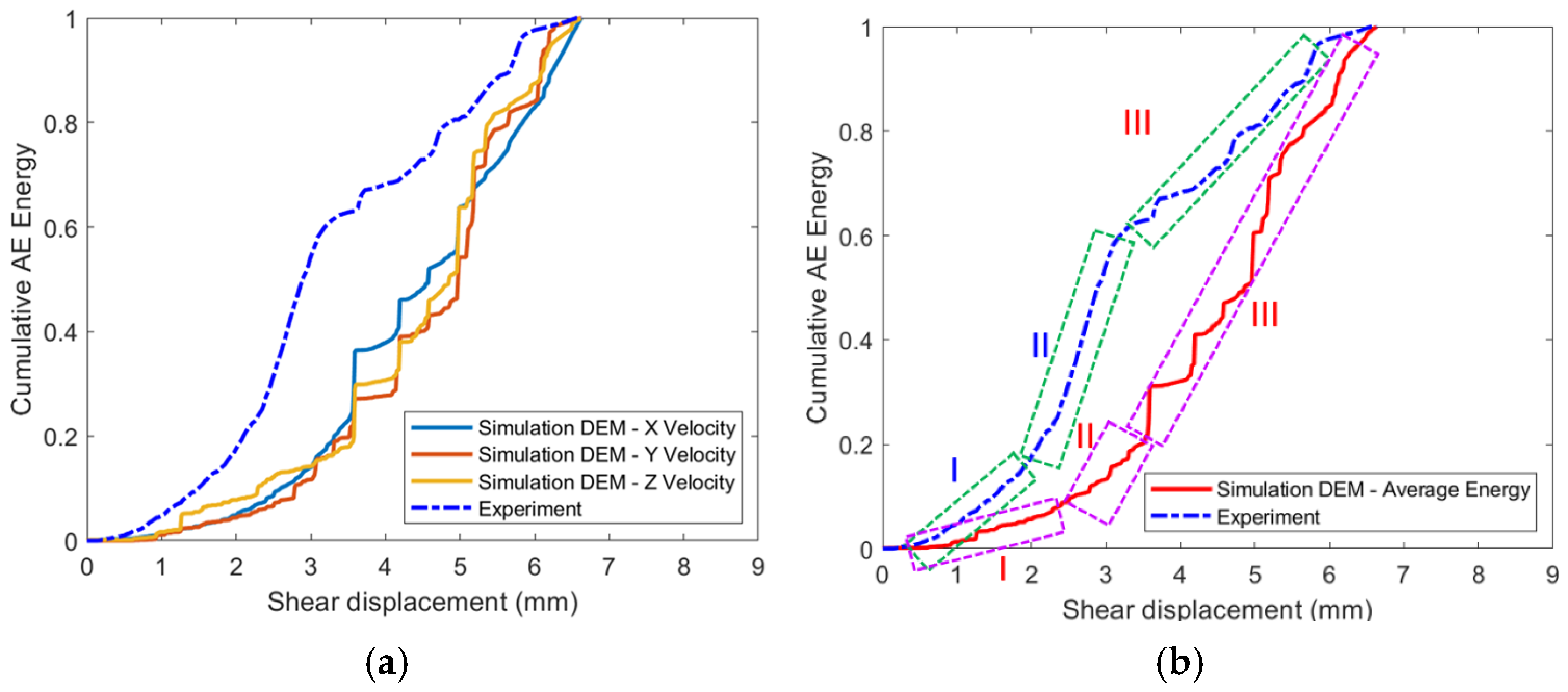
To evaluate the ability of the numerical model to simulate AE, the cumulative AE energy is compared between the experimental and numerical results, using only the experimental measurements from the S8 sensor. In the numerical calculation, the velocity measurements (in the X, Y, and Z directions) were taken at the same position as the S8 sensor in the experiment. This sensor was located on the external surface of the masonry wall, at coordinates X = 0.08125 m and Z = 0.1239 m (where X is the horizontal direction and Z is the vertical direction). In the numerical calculation, the cumulative AE energy was calculated from the measured velocity signal and then normalized for comparison with the experimental results.

Overall, the numerical energy curve exhibited a similar trend to the experimental curve, consisting of three phases, as shown in Figure 22. However, the numerical curve was lower than the experimental one. This difference can be attributed to the lower stiffness observed in the numerical load versus displacement curve (Figure 21) compared to the experimental one. Despite this discrepancy, the numerical model remains robust in its ability to capture the acoustic energy relative to the test results.

It is important to note that AE events are not recorded instantaneously at the moment of crack initiation. Instead, AE signals are generated by the rapid release of elastic energy during micro-crack formation and propagation, and they require a finite time to reach the sensors. This introduces a time delay between the actual cracking event and the detected AE signal. This delay is mainly governed by the wave propagation velocity in the material, the distance between the source of damage and the sensor location, and the heterogeneity of the medium. In addition, instrumental response and signal processing may further contribute to this temporal shift. As a result, a slight discrepancy can exist between the exact time of crack occurrence in the DEM simulations and the corresponding AE event recorded in experiments. This aspect should be considered when interpreting the correlation between simulated fracture evolution and measured AE activity.

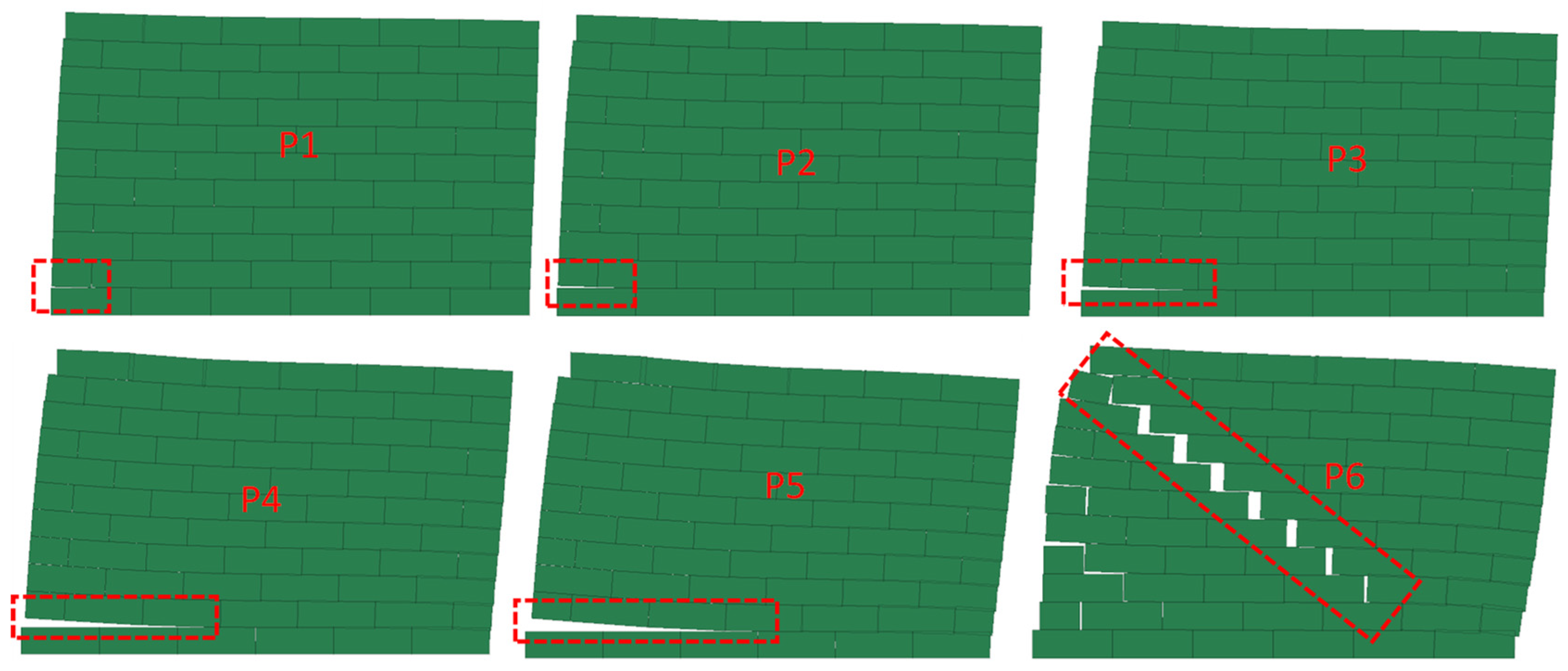
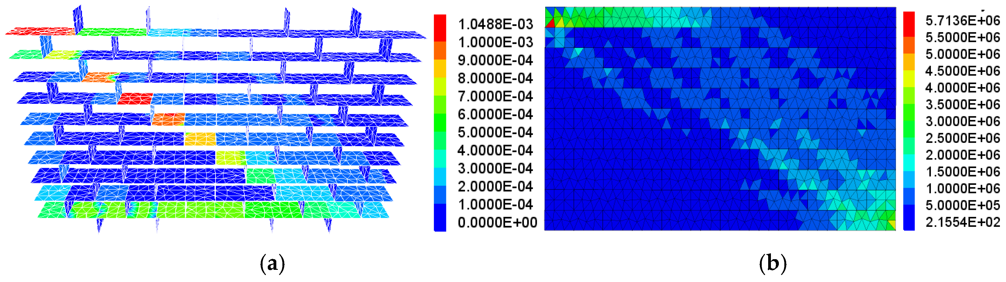
Regarding the failure modes, the wall first cracked in the horizontal joint of the first line in the flexural mode (point P1) (Figure 23). This crack continued to develop and widen, while only a small number of shear cracks initially appeared. However, from point P4 onward, more shear cracks became evident. At point P6 (Figure 24), a yield line with significant cracks formed in the diagonal zone, which explains the sudden drop observed at this point in the load/displacement curve.

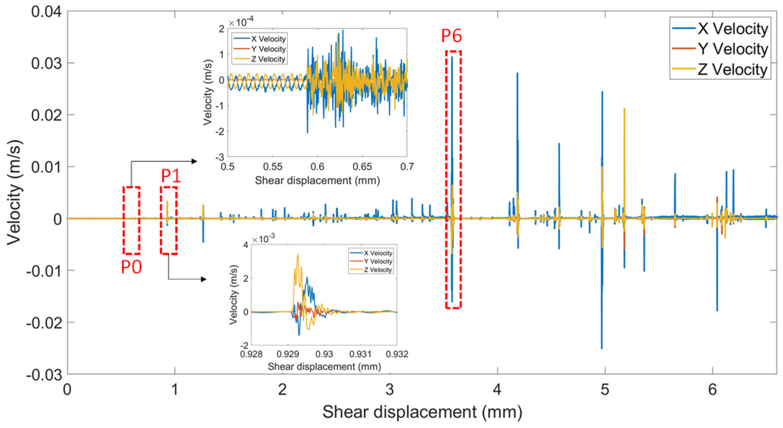
In the numerical model, based solely on the load/displacement curve, the curve remained nearly linear up to point P1, with U = 0.96 mm and F = 37.45 kN. In contrast, the first crack in the experimental test was detected earlier, at U = 0.58 mm and F = 29.23 kN. However, when examining the AE signal obtained from the numerical model, it was observed that the first AE event was detected much earlier, at a displacement of 0.58 mm and F = 23.43 kN, corresponding to 32 cumulative cracks in the masonry wall (point P0 in Figure 25), which is very close to the experimental one.

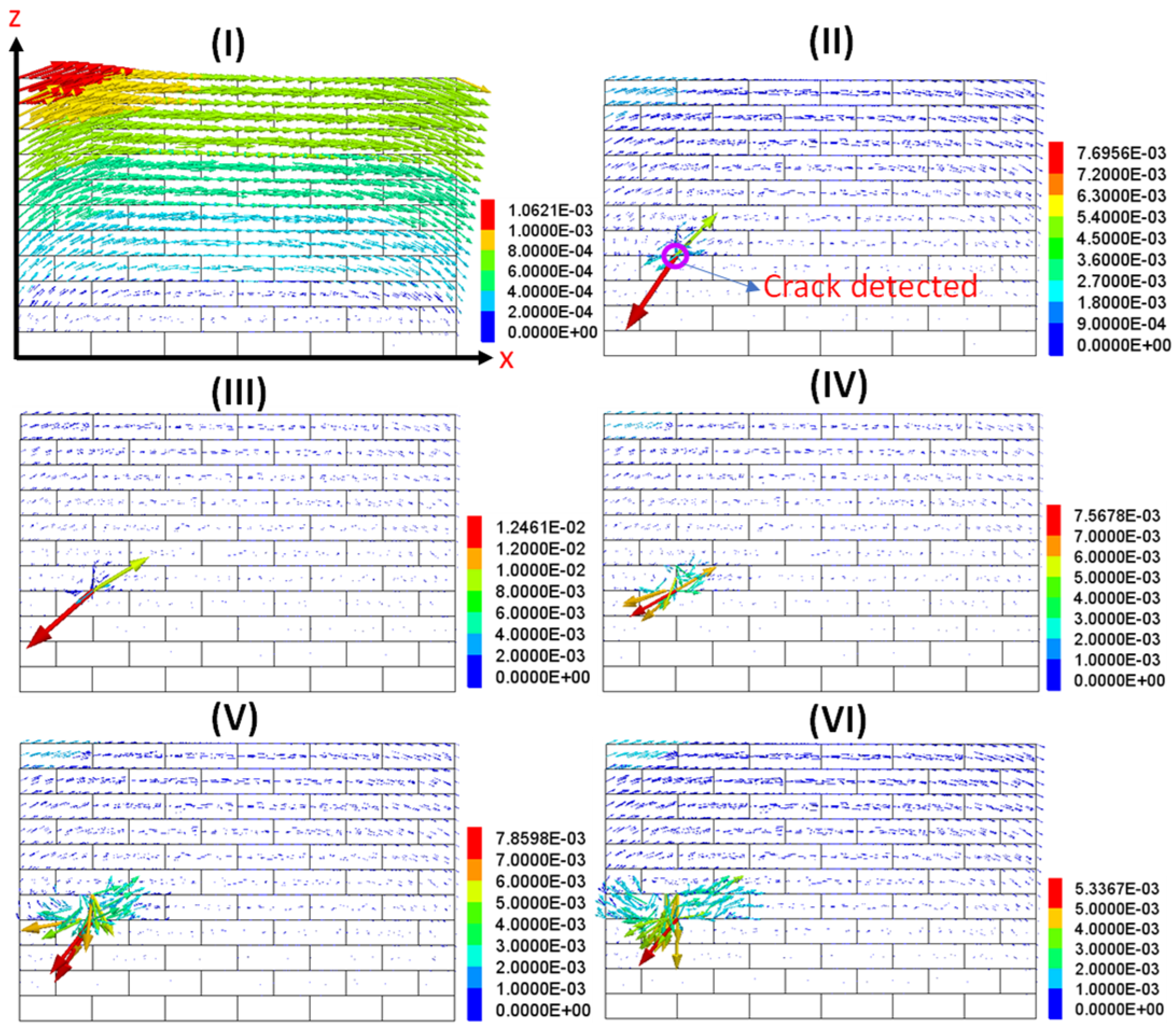
The position of the first crack, detected at a displacement of 0.58 mm, was identified using a tool in the numerical model, which provides the coordinate point x = 0.305 m, y = 0 m, z = 0.425 m. Figure 26 shows a visualization of the velocity vector field before and after the appearance of this crack. Before the crack appears, the maximum velocity was at the loading location (1 mm/s) and progressively decreases in areas further from the load. Once the crack formed, a sudden increase in velocity was observed at the crack location, with speeds reaching up to 12.5 mm/s, significantly higher than the load velocity of 1 mm/s. This velocity was then developed, propagated, and dissipated throughout the structure.

In the study of Carpinteri et al. (2016) [40], the dissipated fracture energy and the emitted energy detected by the AE sensors per unit of fracture surface were compared. In the DEM, the total energy balance can be expressed as the released energy (${\mathrm{W}}_{\mathrm{r}}$), which is the difference between the work done at the model’s boundary and the total stored and dissipated strain energies. While the work of Carpinteri et al. successfully established the energy balance of cracking in concrete-like materials, their approach remains focused on the material scale. In contrast, our work extends these principles to the structural level, accounting for the complex interaction of blocks and joints in a full wall assembly.

$${\mathrm{W}}_{\mathrm{r}}=\mathrm{W}-({\mathrm{U}}_{\mathrm{c}}+{\mathrm{U}}_{\mathrm{b}}+{\mathrm{W}}_{\mathrm{j}}+{\mathrm{W}}_{\mathrm{p}})$$

(4)

where

${\mathrm{W}}_{\mathrm{r}}$ is released energy;

$\mathrm{W}$ is total boundary loading work supplied to the system;

${\mathrm{U}}_{\mathrm{c}}$ is total stored strain energy in material;

${\mathrm{U}}_{\mathrm{b}}$ is total change in potential energy of the system;

${\mathrm{W}}_{\mathrm{j}}$ is total dissipated energy in joint shear; and

${\mathrm{W}}_{\mathrm{p}}$ is total dissipated work in plastic deformation of intact rock.

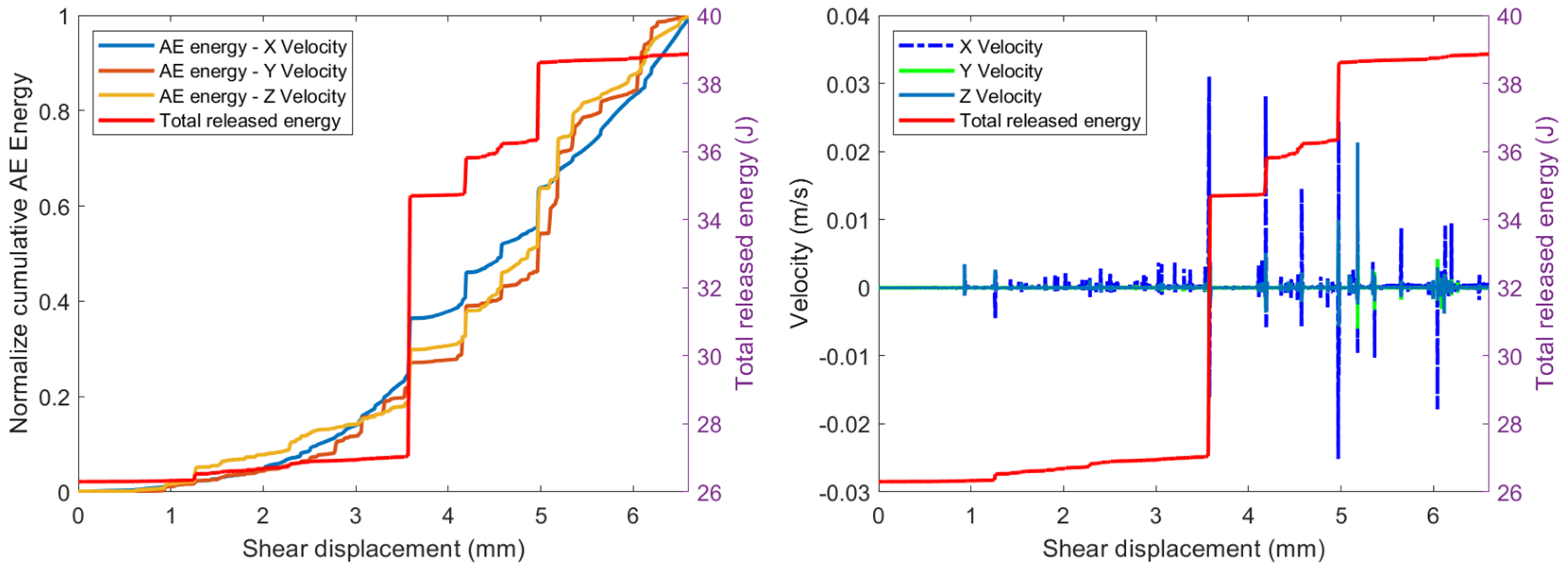
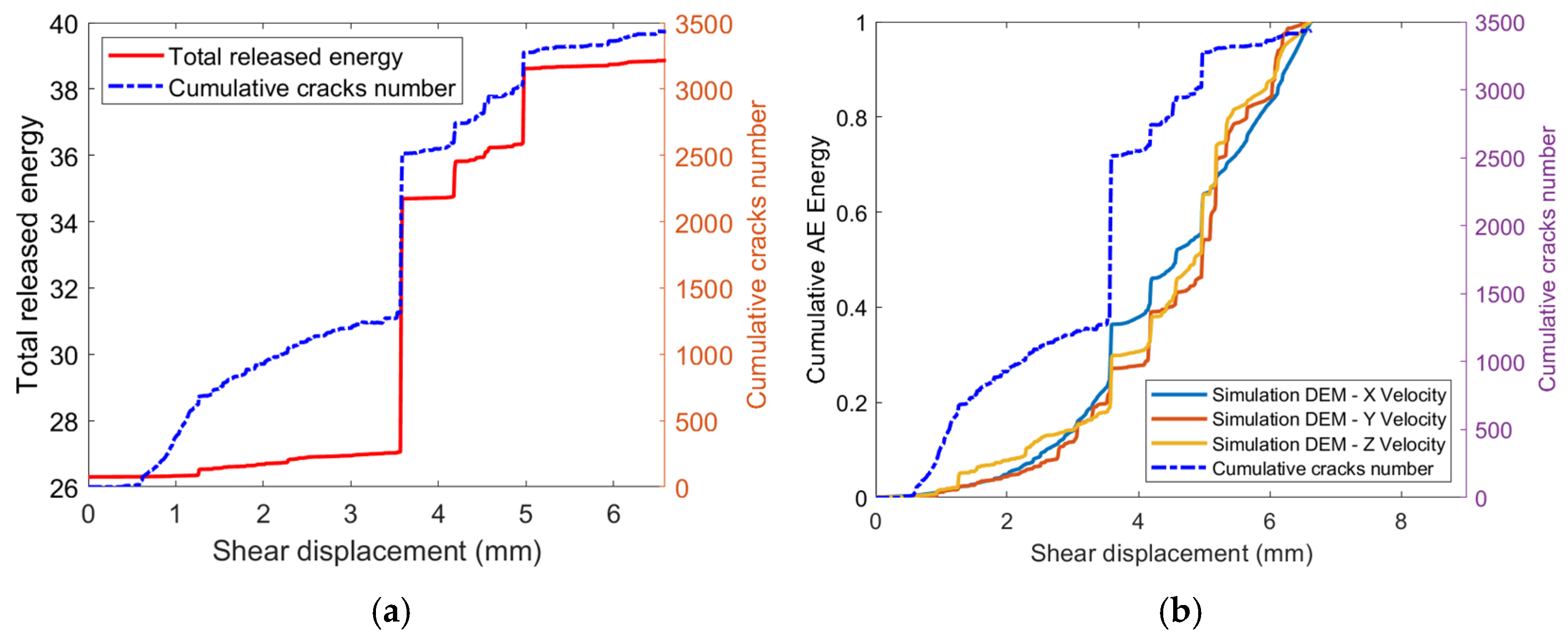
The relationship between the total energy balance (or total released energy) and the amplitude and energy of AE signals is shown in Figure 27. It is observed that a significant increase in the total released energy corresponds to a notable increase in both AE energy and AE amplitude.

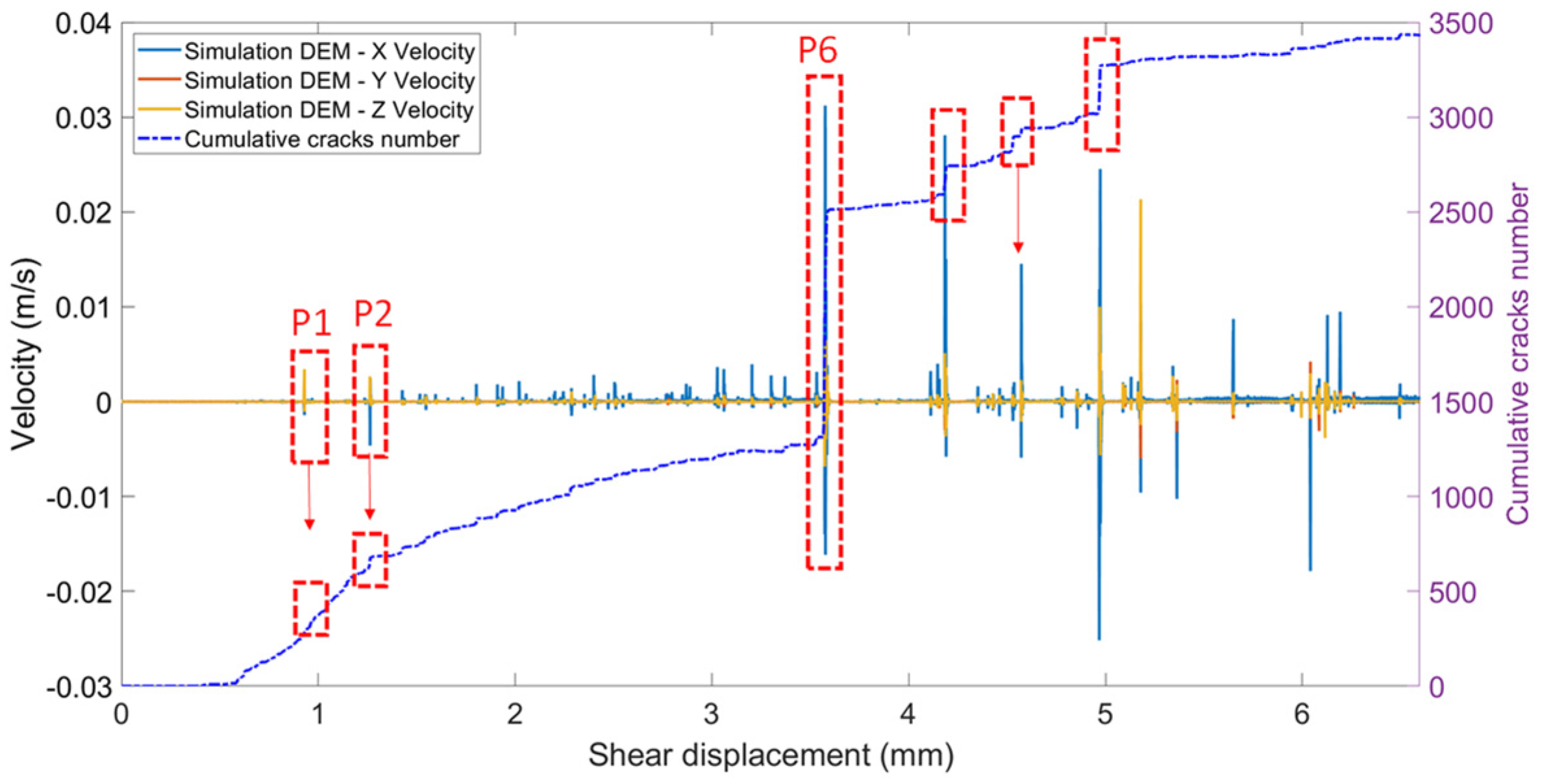
Then, the cumulative number of cracks obtained from the numerical model was used to further analyze the results. Figure 28 shows the cumulative crack count and the measured velocity as a function of the shear displacement. From the result analysis, it was observed that a rapid increase in the number of cracks over a short period (for example, at points P1, P2, and P6) leads to a significant amplitude in the measured velocity, which also corresponds to a considerable release of total energy (Figure 29b). This behavior further explains the generation of elastic waves due to the cracks.

In the literature, there are studies that have demonstrated, through experimental testing, that a snap-back occurs during fracture, and the captured AE energy corresponds to this phenomenon [6,41,42]. However, this does not mean that this phenomenon is validated for all types of brittle materials, nor at the structural scale. In this study, we focus on the rupture of a masonry wall under shear, which occurs at the structural scale. Furthermore, the cracks captured here are at the interfaces between blocks, with no rupture at the block level. While the snap-back phenomenon has been demonstrated at the material scale (once again not for all materials), it has not yet been observed at the structural scale, nor in relation to rupture at the interface level.

The results obtained in this study clearly show that there is no snap-back phenomenon in the force/displacement curve of the masonry wall under shear, either in the experimental tests or in the numerical simulation. In the experimental test, the snapback was not observed in the load/displacement curve. However, the AE energy calculations from the AE signal can still reproduce the acoustic emission well. In the numerical simulation, we have observed that crack propagation occurred suddenly, leading to a catastrophic drop in load capacity before stable crack propagation is established (Figure 21a). This drop in load, as explained in this paper, corresponds to the release of elastic waves, which can be captured by measuring the velocity at the surface. A significant increase in the total energy released was also captured at the time of crack propagation (Figure 29a), which confirm again the physical phenomena reproduced by the numerical model.

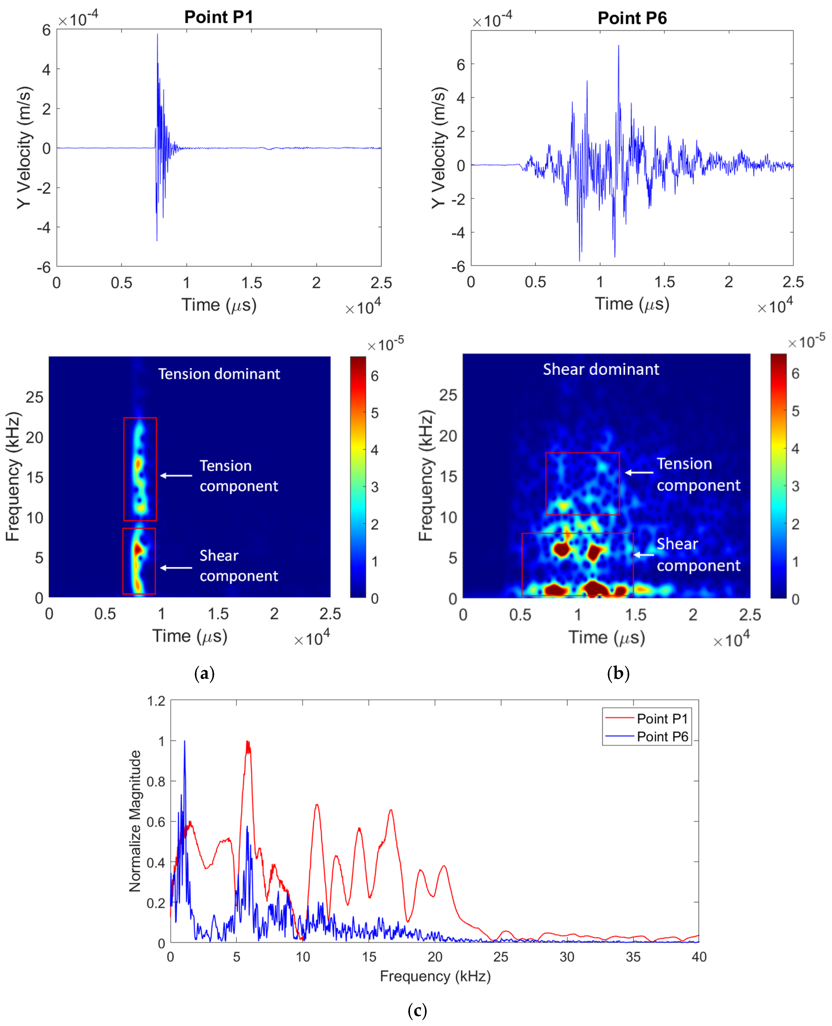
The results show that analyzing the velocity and cumulative AE energy allows for the detection of crack initiation and the intensity of cracking. However, this approach does not provide information about the type of cracks detected. To gain more insight into the crack types, a frequency analysis as a function of time is performed. In the previous section, we observed that the cracks detected at point P1 are primarily caused by bending failure. Cracks at point P6 were mostly associated with shear failure, marked by the formation of a yield line in the diagonal zone. It is important to note that, in both cases, a combination of two types of cracks—tension and shear—occurred. However, point P1 was predominantly governed by tension, while point P6 was primarily dominated by shear.

In the previous section, when studying a single joint, we observed that shear cracks tend to generate lower frequencies than tensile cracks. This same trend was observed for the masonry wall. At point P1, two frequency ranges were identified: low frequencies (from 1.5 kHz to 5.8 kHz) and higher frequencies (from 11.0 kHz to 16.7 kHz) (Figure 30a). Typically, lower frequencies were associated with tensile cracks, while higher frequencies correspond to shear cracks. At point P6, the frequencies were predominantly in the low range, from 1.1 kHz to 5.8 kHz (Figure 30b), although a higher frequency of 10.4 kHz was also detected, but with much lower intensity. Another observation was that the tension-dominant mode produced frequencies over a short time frame, whereas the shear-dominant mode generated frequencies over a longer duration.

The frequency analysis indicates that different fracture mechanisms produce distinct frequency characteristics. In general, tensile-dominant cracking is associated with higher-frequency and shorter-duration responses, whereas shear-dominant cracking tends to generate lower-frequency components over a longer duration. These trends are consistent with the underlying energy release and crack-propagation mechanisms governing each failure mode. It is also acknowledged that the obtained frequency content is influenced not only by the fracture process itself but also by the numerical discretization and model parameters in the DEM framework. In particular, mesh size affects the contact network and stress-wave propagation paths, which can modify both the detected frequency ranges and their amplitudes. Similarly, contact stiffness and damping parameters influence wave transmission and attenuation, thereby affecting the resulting spectral response. Accordingly, the interpretation of AE frequency signatures should consider both the physical fracture mechanisms and the inherent limitations of the numerical model. This provides a more robust basis for evaluating the reliability of the proposed AE simulation approach.

5. Brief Description of Methodology Used

This paper presents a novel method for simulating acoustic emission in masonry walls in shear using the discrete element method. To calibrate the numerical model based on DEM, two steps are proposed:

Step 1: Before studying the acoustic emission phenomenon, the model must first be validated for mechanical behavior. Interface parameters can be characterized through shear and tensile strength tests, and results could be implemented into the numerical model. At the structural scale, model validation is performed by comparing the numerical results with structural tests, focusing on the global force/deflection behavior curve and the failure modes obtained. A local damping value of 0.3 can be used. Mesh convergence should also be conducted.

Step 2: After validating the model in terms of mechanical behavior, the model’s ability to simulate acoustic emission is calibrated. Elastic waves are captured by measuring the velocity on the wall surface. From this signal, various acoustic emission parameters, such as cumulative AE energy or the b-value can be used for calibration. This study specifically addresses the evaluation of cumulative AE energy.

It is acknowledged that the optimal damping coefficient may depend on the modeling scale and the physical phenomena under investigation. At the joint or particle interaction scale, lower damping values may be preferred to better preserve local dynamic effects, while larger-scale structural simulations may require higher damping to ensure numerical stability and computational efficiency. Therefore, the selected value of α = 0.3 should not be considered universally applicable, but rather appropriate for the specific DEM configuration, loading conditions, and AE analysis framework considered in this study.

6. Conclusions

This research presented a novel application of block-based Discrete Element Method (DEM) to simulate acoustic emission (AE) waves in masonry structures at the structural scale. While previous DEM studies on AE were restricted to small-scale material tests, this work successfully modeled damage progression in a large-scale wall panel (1.835 × 1.170 × 0.15 m³), bridging the gap between micro-mechanical modeling and the macro-structural response. Based on the results of this study, several significant outcomes were achieved:

• A major contribution of this work is the optimal numerical calibration of AE and the identification of the critical role played by local damping in capturing elastic waves. While a standard damping ratio of 0.8 is typical for static equilibrium, this study established that a reduced ratio of 0.3 is optimal for AE simulations. This specific value preserves the kinetic energy required for high-fidelity velocity signals while maintaining computational stability, a technical guideline not previously addressed in the literature.
• Moreover, the model validation of structural-scale predictive capability was demonstrated. In particular, the proposed model demonstrated strong agreement with existing experimental data, accurately capturing the force–displacement response and the cumulative AE energy curves. This confirms that block-based DEM is a robust tool for predicting failure mechanisms in heterogeneous masonry where traditional continuum-based methods often fail.
• What is more, this research was able to differentiate failure modes using AE. Through frequency analysis, the model successfully distinguished between tensile and shear cracking modes based on their signal signatures. This outcome is significant for structural health monitoring (SHM), as it provides a theoretical framework to identify the physical nature of internal damage using only external vibration data. In a real-world scenario, this allows structural engineers to categorize the severity of damage, for instance, identifying sudden shear failure modes in a wall panel, which are often more catastrophic than gradual tensile cracking.
• Finally, the study proves the feasibility of using the DEM as a “virtual sensor” platform. By simulating the AE response of large structures, engineers can pre-calibrate physical sensor layouts and better understand the complex attenuation and reflection of waves across mortar joints, which are critical for accurate crack localization in real-world masonry infrastructure. Due to the model’s ability to simulate how mortar joints reflect and attenuate signals, engineers can “test” different sensor layouts virtually to ensure that critical internal damage zones are within the detection range of the physical equipment.

Overall, the methodology developed as part of this research provides a powerful, computationally efficient tool for the non-destructive assessment of masonry structures, offering deeper insights into damage initiation and propagation than experimental methods alone can provide. Also, the study successfully fills a significant gap in the literature by demonstrating that the DEM is an effective predictive tool for structural-scale failure analysis and AE monitoring in heterogeneous masonry. The study provides a framework for the enhanced safety evaluation of masonry infrastructure. By utilizing the proposed structural-scale DEM model, engineers can simulate the acoustic emission (AE) signatures of specific failure mechanisms before they become visible to the naked eye. This capability is particularly vital for the assessment of heritage structures, where invasive testing is prohibited. Furthermore, the ability to correlate simulated AE energy and frequency with internal crack progression allows for the definition of ‘early-warning’ thresholds. These thresholds can inform automated health monitoring systems, identifying a transition from stable micro-cracking to unstable structural failure, thereby significantly improving the reliability of safety assessments in the field.

References

1. Lee, H.L.; Kim, J.S.; Hong, C.H.; Cho, D.K. Ensemble learning approach for the prediction of quantitative rock damage using various acoustic emission parameters. Appl. Sci. 2021, 11, 4008. [Google Scholar] [CrossRef]
2. Aggelis, D.G.; Kordatos, E.Z.; Matikas, T.E. Acoustic emission for fatigue damage characterization in metal plates. Mech. Res. Commun. 2011, 38, 106–110. [Google Scholar] [CrossRef]
3. Hamstad, M.A. A review: Acoustic emission, a tool for composite-materials studies. Exp. Mech. 1986, 26, 7–13. [Google Scholar] [CrossRef]
4. Ren, H.; Li, T.; Ning, J.; Song, S. Analysis of damage characteristics of steel fiber-reinforced concrete based on acoustic emission. Eng. Fail. Anal. 2023, 148, 107166. [Google Scholar] [CrossRef]
5. Qin, F.; Sheng, D.; Chai, Z.; Huo, X. chanism analysis of steel-polypropylene fiber reinforced recycled concrete based on acoustic emission and digital image correlation. Eng. Fail. Anal. 2024, 161, 108315. [Google Scholar] [CrossRef]
6. Verstrynge, E.; Lacidogna, G.; Accornero, F.; Tomor, A. A review on acoustic emission monitoring for damage detection in masonry structures. Constr. Build. Mater. 2021, 268, 121089. [Google Scholar] [CrossRef]
7. Szabó, S.; Funari, M.F.; Lourenço, P.B. Masonry patterns’ influence on the damage assessment of URM walls: Current and future trends. Dev. Built Environ. 2023, 13, 100119. [Google Scholar] [CrossRef]
8. Basha, S.H.; Guo, Z.X.; Xie, X. Effect of structural bonding patterns on mechanical characteristics of clay brick masonry under different loadings using digital image correlation technique. J. Mater. Civ. Eng. 2022, 34, 04022302. [Google Scholar] [CrossRef]
9. Peng, S.; Parent, T.; Sbartaï, Z.M.; Morel, S. Damage monitoring of masonry structures using the acoustic emission technique–From tensile and shear characterization tests to shear wall tests. Eng. Fract. Mech. 2024, 296, 109845. [Google Scholar] [CrossRef]
10. Livitsanos, G.; Shetty, N.; Verstrynge, E.; Wevers, M.; Van Hemelrijck, D.; Aggelis, D.G. Shear failure characterization in masonry components made with different mortars based on combined NDT methods. Constr. Build. Mater. 2019, 220, 690–700. [Google Scholar] [CrossRef]
11. Li, S.; Wu, Y.; Li, W.; Li, P. Shear test on damage evolution of brick masonry based on acoustic emission technique. Constr. Build. Mater. 2021, 273, 121782. [Google Scholar] [CrossRef]
12. Peng, S.; Sbartaï, Z.M.; Parent, T. Mechanical damage evaluation of masonry under tensile loading by acoustic emission technique. Constr. Build. Mater. 2020, 258, 120336. [Google Scholar] [CrossRef]
13. Cundall, P.A.; Strack, O.D.L. The development of constitutive laws for soil using the distinct element method. Numer. Methods Geomech. 1979, 1, 289–317. [Google Scholar]
14. Lemos, J.V. Explicit codes in geomechanics—FLAC, UDEC and PFC. In Innovative Numerical Modelling in Geomechanics; CRC Press: Boca Raton, FL, USA, 2012; pp. 299–315. [Google Scholar] [CrossRef]
15. Cundall, P.A. Distinct element models of rock and soil structure. In Anal. Comput. Methods Eng. Rock Mech.; Brown, E.T., Ed.; George Allen Unwin: London, UK, 1987; pp. 129–163. [Google Scholar]
16. Lemos, J.V. Discrete element modeling of masonry structures. Int. J. Archit. Herit. 2007, 1, 190–213. [Google Scholar] [CrossRef]
17. Schiavoni, M.; Giordano, E.; Roscini, F.; Clementi, F. Numerical modeling of a majestic masonry structure: A comparison of advanced techniques. Eng. Fail. Anal. 2023, 149, 107293. [Google Scholar] [CrossRef]
18. Ita, P.; Santa-Cruz, S.; Daudon, D.; Tarque, N. Numerical and experimental pseudo-static study on block arrangement effects in traditional dry-stone walls for out-of-plane mechanical behavior evaluation. Eng. Fail. Anal. 2024, 166, 108900. [Google Scholar] [CrossRef]
19. Tan, X.; Konietzky, H.; Chen, W. Numerical simulation of heterogeneous rock using discrete element model based on digital image processing. Rock Mech. Rock Eng. 2016, 49, 4957–4964. [Google Scholar] [CrossRef]
20. Hazzard, J.F.; Young, R.P. Simulating acoustic emissions in bonded-particle models of rock. Int. J. Rock Mech. Min. Sci. 2000, 37, 867–872. [Google Scholar] [CrossRef]
21. Ji, S.; Di, S. Discrete element modeling of acoustic emission in rock fracture. Theor. Appl. Mech. Lett. 2013, 3, 021009. [Google Scholar] [CrossRef]
22. Rucka, M.; Knak, M.; Nitka, M. A study on microcrack monitoring in concrete: Discrete element method simulations of acoustic emission for non-destructive diagnostics. Eng. Fract. Mech. 2023, 293, 109718. [Google Scholar] [CrossRef]
23. Bui, T.T.; Limam, A.; Sarhosis, V. Failure analysis of masonry wall panels subjected to in-plane and out-of-plane loading using the discrete element method. Eur. J. Environ. Civ. Eng. 2021, 25, 876–892. [Google Scholar] [CrossRef]
24. Bui, T.T.; Limam, A.; Bui, Q.B. Characterisation of vibration and damage in masonry structures: Experimental and numerical analysis. Eur. J. Environ. Civ. Eng. 2014, 18, 1118–1129. [Google Scholar] [CrossRef]
25. Bui, T.T.; Limam, A.; Sarhosis, V.; Hjiaj, M. Discrete element modelling of the in-plane and out-of-plane behaviour of dry-joint masonry wall constructions. Eng. Struct. 2017, 136, 277–294. [Google Scholar] [CrossRef]
26. Pulatsu, B.; Erdogmus, E.; Lourenço, P.B.; Lemos, J.V.; Tuncay, K. Simulation of the in-plane structural behavior of unreinforced masonry walls and buildings using DEM. In Structures; Elsevier: Amsterdam, The Netherlands, 2020; Volume 27, pp. 2274–2287. [Google Scholar]
27. Zhao, Y.; Zhao, Q.; Yang, T.; Chen, Y.; Zhang, P.; Liu, H. Investigation of crack propagation and acoustic emission characteristics in jointed rock under freeze–thaw cycles based on DEM. Int. J. Min. Sci. Technol. 2025, 35, 1171–1195. [Google Scholar] [CrossRef]
28. Beskopylny, A.N.; Stel’makh, S.A.; Shcherban’, E.M.; Dolgov, V.; Beskopylny, N.; Elshaeva, D.; Chernil’nik, A.; Panfilov, I.; Razveeva, I. Defects Identification and Crack Depth Deter-mination in Porous Media on the Brick Masonry Example Using Ultrasonic Methods: Numerical Analysis and Machine Learning. J. Compos. Sci. 2025, 9, 267. [Google Scholar]
29. Bravo, R.; Pérez-Aparicio, J.L. Improving damage detection in masonry bridges: A combination of finite–discrete element method and genetic algorithms. In Structures; Elsevier: Amsterdam, The Netherlands, 2025; Volume 81, p. 110279. [Google Scholar]
30. Cundall, P.A. Formulation of a three-dimensional distinct element model—Part I. A scheme to detect and represent contacts in a system composed of many polyhedral blocks. Int. J. Rock Mech. Min. Sci. Geomech. Abstr. 1988, 25, 107–116. [Google Scholar] [CrossRef]
31. Venzal, V.; Morel, S.; Parent, T.; Dubois, F. Frictional cohesive zone model for quasi-brittle fracture: Mixed-mode and coupling between cohesive and frictional behaviors. Int. J. Solids Struct. 2020, 198, 17–30. [Google Scholar] [CrossRef]
32. Boukham, A.; Venzal, V.; Parent, T.; Morel, S.; Dubois, F.; Solbes, B. 3D hybrid modeling approach combining the finite and discrete element methods: Validation based on masonry shear wall tests. Int. J. Solids Struct. 2024, 289, 112638. [Google Scholar] [CrossRef]
33. Itasca Consulting Group Inc. 3DEC Three Dimensional Distinct Element Code 2013; Itasca Consulting Group Inc.: Minneapolis, MN, USA, 2013. [Google Scholar]
34. Zhang, L.; Ren, T.; Li, X.; Tan, L. Acoustic emission, damage and cracking evolution of intact coal under compressive loads: Experimental and discrete element modelling. Eng. Fract. Mech. 2021, 252, 107690. [Google Scholar] [CrossRef]
35. Mandal, D.D.; Bentahar, M.; El Mahi, A.; Brouste, A.; El Guerjouma, R.; Montresor, S.; Cartiaux, F.-B.; Semiao, J. Acoustic emission monitoring of damage modes in reinforced concrete beams by using narrow partial power bands. Sci. Rep. 2024, 14, 27082. [Google Scholar] [CrossRef] [PubMed]
36. Yu, X.; Bentahar, M.; Mechri, C.; Montrésor, S. Passive monitoring of nonlinear relaxation of cracked polymer concrete samples using acoustic emission. J. Acoust. Soc. Am. 2019, 146, EL323–EL328. [Google Scholar] [CrossRef]
37. Yu, X.; Montrésor, S.; Bentahar, M.; Mechri, C. Cluster analysis of acoustic emission signals for the damage pattern recognition of polymer concrete. Appl. Acoust. 2023, 211, 109533. [Google Scholar] [CrossRef]
38. Sun, Q.; Dai, S.; Hao, R.; Xiao, Y. Study on mechanical properties and acoustic emission characteristics of composite rock mass with different thicknesses of weak interlayer. Sci. Rep. 2024, 14, 27835. [Google Scholar] [CrossRef]
39. Peng, S. Advance on Non-Destructive Evaluation Methodologies for the Material Characterization and Damage Monitoring of Masonry Structures. Ph.D. Thesis, Université de Bordeaux, Bordeaux, France, 2022. [Google Scholar]
40. Carpinteri, A.; Lacidogna, G.; Corrado, M.; Di Battista, E. Cracking and crackling in concrete-like materials: A dynamic energy balance. Eng. Fract. Mech. 2016, 155, 130–144. [Google Scholar] [CrossRef]
41. Friedrich, L.F.; Tanzi, B.N.R.; Colpo, A.B.; Sobczyk, M.; Lacidogna, G.; Niccolini, G.; Iturrioz, I. Analysis of acoustic emission activity during progressive failure in heterogeneous materials: Experimental and numerical investigation. Appl. Sci. 2022, 12, 3918. [Google Scholar] [CrossRef]
42. Lacidogna, G.; Accornero, F.; Carpinteri, A. Influence of snap-back instabilities on Acoustic Emission damage monitoring. Eng. Fract. Mech. 2019, 210, 3–12. [Google Scholar] [CrossRef]
Figure 1. Behavior law of joint under shear and tension: (a) shear behavior; (b) tension behavior [25].
Buildings 16 01990 g001
Figure 2. Representation of block in the DEM: (a) mesh of block B1; (b) specimen under shear; (c) specimen under direct tension.
Buildings 16 01990 g002
Figure 3. Common plan (c-p) between two blocks by Cundall (1988) [30].
Buildings 16 01990 g003
Figure 4. Influence of local damping (after broken bond in joint) on the (a) convergence speed and (b) kinetic energy.
Buildings 16 01990 g004
Figure 5. Influence of local damping (after broken bond in joint) on the load/displacement curve.
Buildings 16 01990 g005
Figure 6. Influence of local damping (after broken bond in joint) on the load/displacement curve.
Buildings 16 01990 g006aBuildings 16 01990 g006b
Figure 7. (a) Shear stress at joint; (b) cumulative number of cracks (cumulative AE event) as a function of the horizontal displacement.
Buildings 16 01990 g007
Figure 8. Parameters of AE.
Buildings 16 01990 g008
Figure 9. (a) Y velocity versus and cumulative crack number versus shear displacement; (b) cumulative AE energy and cumulative crack number versus shear displacement.
Buildings 16 01990 g009
Figure 10. (a) Tensile stress and cumulative crack number versus vertical displacement; (b) cumulative AE energy and cumulative crack number versus vertical displacement.
Buildings 16 01990 g010
Figure 11. Waveform AE signal and wavelet scalogram using time–frequency of AE signal for tensile crack, shear crack, and mixed mode tension/shear case.
Buildings 16 01990 g011
Figure 12. Mesh size corresponds to number of sub-contacts: (a) N = 8; (b) N = 18; (c) N = 32; (d) N = 50; (e) N = 98.
Buildings 16 01990 g012
Figure 13. Influence of mesh size on the shear stress/shear displacement curve: (a) from 0 to 0.04 mm; (b) from 0.033 mm to 0.04 mm.
Buildings 16 01990 g013
Figure 14. Influence of mesh size on the following: (a) y velocity measurement; (b) frequency of velocity measurement.
Buildings 16 01990 g014
Figure 15. Normalization of cumulative AE energy and cumulative crack number with mesh size of (a) N = 32 and (b) N = 98.
Buildings 16 01990 g015
Figure 16. Frequency obtained with tensile loading and shear loading for (a) N = 32 and (b) N = 98.
Buildings 16 01990 g016
Figure 17. Test setup and position of eight AE sensors from Peng et al. (2024) [9] (red line is crack line).
Buildings 16 01990 g017
Figure 18. Mesh of blocks (a,b) and joints (c) in the DEM (mesh size of 50 mm).
Buildings 16 01990 g018
Figure 19. Influence of local damping on the load/displacement curve of masonry wall: (a) global curve; (b) zoomed curve.
Buildings 16 01990 g019
Figure 20. (a) Wall with mesh size of 75 mm and 30 mm; (b) load against displacement curve.
Buildings 16 01990 g020
Figure 21. (a) Comparison between the experimental and the numerical load/displacement curve; (b) numerical cumulative crack number and numerical load/displacement curve.
Buildings 16 01990 g021
Figure 22. Comparison between the experimental and the numerical results: normalize cumulative AE energy with (a) all curve; (b) average curve.
Buildings 16 01990 g022
Figure 23. Crack propagation of the masonry wall in numerical model (Deform factor of 15).
Buildings 16 01990 g023
Figure 24. At point P6, (a) joint shear displacement (unit in m); (b) block Von Mises Equivalent Stress (unit in Pa).
Buildings 16 01990 g024
Figure 25. Velocity monitored at Sensor 8 in numerical simulation.
Buildings 16 01990 g025
Figure 26. Velocity magnitude observed numerically before and after the crack at U = 0.58 mm (unit in m/s).
Buildings 16 01990 g026
Figure 27. AE signal amplitude, normalizing cumulative AE energy and total released energy (total energy balance).
Buildings 16 01990 g027
Figure 28. Velocity monitored at Sensor 8 and cumulative number of cracks in the numerical model.
Buildings 16 01990 g028
Figure 29. Results from the computational model: (a) total released energy (energy in J) against shear displacement; (b) cumulative AE energy and cumulative number of cracks against shear displacement.
Buildings 16 01990 g029
Figure 30. Waveform AE signal and wavelet scalogram using time–frequency of AE signal: (a) point P1; (b) point P6; (c) FFT.
Buildings 16 01990 g030