Multi-Velocity Ceiling Diffuser for Orthopedic Procedures or Ventilation: An Integrated CFD, Performance Assessment, and Surrogate Modeling Framework

Abstract

Operating room ventilation is a key engineering factor in maintaining clean air environments. This study presents an integrated three-part methodology combining Computational Fluid Dynamics parametric analysis, performance assessment with effect size analysis and multi-criteria decision analysis using quantitative engineering metrics, and surrogate modeling for thermal effect propagation in an orthopedic operating room. Simulations were conducted in ANSYS Fluent 2020 R₂, benchmarking an existing local operating room against an ASHRAE 170-2021 compliant model, followed by parametric evaluation of four ceiling inlet configurations. The existing system exhibited critically low velocities (0.05–0.10 m/s) with a coefficient of variation of 0.73, indicating severe flow non-uniformity. The proposed Multi-Velocity Ceiling Diffuser—featuring a high-velocity core (0.40 m/s) over the surgical area and a low-velocity peripheral frame (0.20 m/s)—achieved 85% coverage of the ASHRAE-recommended velocity range (0.20–0.30 m/s), a coefficient of variation of 0.14 (81% improvement), and 62 air changes per hour, representing an 86% reduction in supply airflow compared to a full-ceiling system. Effect size analysis confirmed that MVCD performance shows large practical differences from smaller inlet designs (Cohen’s d ≥ 0.41) and negligible difference from full-ceiling systems (Cohen’s d = 0.05). Multi-criteria decision analysis—with feasibility and cost quantified using engineering estimates (ductwork area, downtime days, standardized cost data)—ranked MVCD as optimal under the modeled assumptions (composite score = 0.84), outperforming the existing system (0.59) and full-ceiling design (0.51). To address the isothermal assumption limitation, a Random Forest surrogate model was implemented as a differentiable approximation strategy for parametric uncertainty propagation. Under non-isothermal conditions, the MVCD is predicted to maintain a spatial median velocity of 0.19 m/s (5th–95th percentile range: 0.17–0.21 m/s) and 71% ASHRAE compliance (parameter sampling range across literature-derived distributions: 63–78%). Achieving ASHRAE velocity criteria is an engineering surrogate for ventilation effectiveness; the relationship between these metrics and clinical infection outcomes depends on multiple factors beyond airflow, including surgical technique, patient factors, and antimicrobial prophylaxis. No clinical inference is permitted from the present results. Experimental measurement in a physical MVCD-equipped operating room is required to validate these predictions prior to clinical implementation.

1. Introduction

The pursuit of surgical sterility is a cornerstone of modern medicine, yet operating rooms remain challenging environments for contamination control [1]. Surgical site infections (SSIs) are a major clinical and economic burden, causing a significant percentage of hospital-acquired infections and leading to prolonged hospitalization, additional patient distress, and increased costs [1]. However, this study does not directly model pathogen transport or infection risk. Rather, we evaluate ventilation performance using established engineering metrics (velocity, uniformity, ASHRAE compliance) that serve as design surrogates. The relationship between these metrics and clinical infection outcomes is complex and depends on multiple factors beyond airflow, including surgical technique, patient factors, and antimicrobial prophylaxis [2]. Control of indoor air quality is therefore critical, a task largely left to the Operating Room (OR) ventilation systems. These systems are designed not only for comfort, but also for safety, to create a sterile environment through the control of temperature, humidity, and, most importantly, airborne particle movement and concentration [3].

The efficiency of ventilation systems has been a topic of detailed research. The basis of OR airflow knowledge was established by early experimental work such as that of Mukhaiber [2]. Computational Fluid Dynamics (CFD) has since then transformed this field, allowing for careful, three-dimensional analysis. Previous CFD studies have examined various factors: Rahate and Sarode [4] demonstrated that an inclined air distribution system (30–45°) could overcome obstacles created by people and lights, and Agirman et al. [5] found that air outlet location had a comparatively minor influence compared to inlets. Excellence of advanced systems like Laminar Airflow (LAF) and Temperature-controlled Airflow (TCAF) over conventional turbulent mixing in reducing colony-forming units (CFU) has been shown by Alsved et al. [6]. Further, Sadrizadeh et al., have compared several laminar ventilation conditions numerically, consistently pointing towards performance benefits of centralized ceiling inlets over the surgical area [7,8,9].

Despite extensive research, a gap often exists between theoretical design recommendations and practical implementation in hospitals, particularly in resource-constrained settings. Local operating rooms may not always conform to approved design codes during construction or operation, potentially compromising ventilation effectiveness and patient safety. This study addresses this gap by integrating two complementary research strands: quantitative benchmarking against international standards and systematic parametric analysis of inlet designs. The first contribution moves beyond comparative theory to provide a stark, quantitative estimate of a specific local OR against an international benchmark, actually clearly quantifying its deficits. The second contribution extends the seminal work of Moreno et al. [10], and Sadrizadeh et al. [7,11] by conducting systematic parametric analysis of intake designs in an effort to identify the optimal setup for establishing a sterile operating space. But still, ideal ventilation is controversial, new high-quality evidence challenging the routine effectiveness of expensive LAF systems to prevent SSIs in orthopedic surgery [12].

Despite the methodological rigor of CFD-based ventilation studies, a critical limitation persists: nearly all published work assumes isothermal conditions, omitting the thermal plumes generated by surgical staff (80–100 W per person) and equipment [13,14]. These buoyancy-driven flows can significantly disrupt unidirectional airflow, potentially reducing the protective effect predicted by isothermal simulations [15,16]. Recent experimental studies have shown that thermal effects reduce velocity uniformity by 15–30% compared to isothermal predictions [17], yet most design recommendations continue to rely on isothermal CFD alone.

This study addresses this gap through a three-part integrated methodology:

Part 1—Isothermal CFD Benchmarking and Parametric Analysis: Following established methods [7,8,9,10,11], four ceiling inlet configurations are evaluated under idealized isothermal conditions to identify the Multi-Velocity Ceiling Diffuser (MVCD) as the optimal balance of performance and feasibility.

Part 2—Performance Assessment and Multi-Criteria Decision Analysis: Beyond qualitative CFD comparisons, we apply effect size analysis (Cohen’s d) and multi-criteria decision analysis (MCDA) to quantify practical differences between configurations and account for implementation constraints.

Part 3—Surrogate Modeling for Thermal Effect Prediction: To address the isothermal limitation, a Random Forest surrogate model is developed using literature-derived correlations. This model approximates expected velocity fields under non-isothermal conditions and provides 95% prediction intervals that quantify uncertainty propagation.

This integrated framework represents a methodological advance over conventional CFD studies, which typically present deterministic isothermal results without uncertainty quantification. By combining parametric CFD, effect size-based performance assessment, and surrogate modeling for thermal effect uncertainty propagation, we provide a structured approach for OR ventilation design that is both rigorous and practically applicable. It is important to note that the machine learning component functions as a surrogate approximator of literature-derived correlations, not as a discovery tool for new physical relationships.

2. Materials and Methods

2.1. Isothermal CFD Analysis

2.1.1. Mathematical Formulation and Turbulence Model

The airflow simulation model is formulated based on the fundamental conservation principles of mass, momentum, and energy. The three-dimensional governing equations of airflow are derived from these principles and expressed in a unified general transport formulation that accounts for transient, convective, diffusive, and source terms [18,19]:

$${\displaystyle \frac{\partial \left(\mathsf{\rho }\mathrm{\varnothing }\right)}{\partial t}}+\nabla .\left(\mathsf{\rho }\mathrm{\varnothing }\overline{V}\right)=\nabla .\left({\Gamma }_{ø}\nabla \varnothing \right)+S_{\varnothing }$$

(1)

where ρ is the air density, $\overrightarrow{V}$ denotes the air velocity vector, $\mathrm{\varnothing }$ represents the transported quantity, ${\Gamma }_{ø}$ is the (effective) diffusion coefficient of $\mathrm{\varnothing }$, and $S_{ø}$ is the corresponding source term. It is to be noted that Equation (1) presents the general transport equation in simplified form; the full tensor notation used in the solver includes the stress tensor components for momentum equations [19].

The airflow simulation in this study is conducted under isothermal conditions, with a constant air density throughout the computational domain. Consequently, the energy equation is not solved, and the airflow is treated as incompressible. Furthermore, pollutant or species transport is not considered in the present study. Under these assumptions, the airflow behavior is governed solely by the conservation equations of mass ($\mathrm{\varnothing }=1$ and ${\Gamma }_{ø}=0$) and momentum ($\mathrm{\varnothing }$ represents each of the three velocity components $\mathrm{u},\mathrm{ }\mathrm{v},\mathrm{ }\mathrm{a}\mathrm{n}\mathrm{d}\mathrm{ }\mathrm{w} \mathrm{a}\mathrm{n}\mathrm{d} {\Gamma }_{ø}=\mathsf{\mu }$), which are expressed using the general transport formulation.

Regarding turbulence modeling, the Reynolds-averaged Navier–Stokes (RANS) framework requires closure of the Reynolds stress tensor, which may be accomplished either through Reynolds stress models (RSMs) or by adopting the eddy-viscosity hypothesis. Among eddy-viscosity-based turbulence models, the two-equation k -ε formulations are widely employed in engineering applications and indoor airflow simulations owing to their computational efficiency and numerical robustness. These models solve transport equations for the turbulent kinetic energy k and its dissipation rate ε with the turbulent viscosity defined as:

$${\mathsf{\mu }}_t=\mathsf{\rho }{C}_{\mathsf{\mu }}{\displaystyle \frac{k^2}{\mathsf{\epsilon }}}$$

(2)

The realizable k-ε model was selected over Reynolds Stress Models (RSMs) or Large Eddy Simulation (LES) due to computational constraints associated with the parametric study (four configurations × mesh sensitivity × validation cases). While RSMs or LES could potentially resolve finer turbulent structures, particularly around obstacles and in recirculation zones, the realizable k-ε model has been extensively validated for mean indoor airflow predictions in operating rooms [7,8,20,21,22,23] and provides an acceptable balance between accuracy and computational cost for comparative parametric studies. However, users should note that RANS models inherently smooth small-scale turbulent fluctuations, which may affect the prediction of local flow disturbances near staff and equipment.

A limitation of the realizable k-ε model is its known tendency to overpredict turbulent mixing in buoyancy-driven flows (thermal plumes) by approximately 15–30% in occupied spaces compared to experimental measurements [18,20]. This bias arises from the eddy viscosity assumption, which can overestimate turbulent diffusion in regions with strong buoyancy gradients. The verification against non-isothermal CFD (Section 3.3.5) uses the same k-ε model as ground truth, meaning any systematic bias in the CFD is inherited by the surrogate. Quantitative estimate: For staff-adjacent zones (within 0.5 m), velocity magnitudes may be underpredicted by 0.01–0.03 m/s relative to physical reality; while in the central surgical zone (away from thermal plumes), the bias is expected to be smaller (<0.01 m/s). Readers should interpret non-isothermal predictions as approximations conditional on the chosen turbulence model, with confidence highest in the surgical zone and lower near staff members.

2.1.2. CFD Model Setup

The computational study was performed using ANSYS Fluent 2020 R2 (ANSYS Inc., Canonsburg, PA, USA). The geometries for all models, including the operating table, surgical staff, major equipment, and ventilation openings, were constructed within the ANSYS ‘Design Modeler module’ (version 2020 R2). A polyhedral mesh was generated for its advantages in convergence and solution stability. A systematic mesh sensitivity analysis was performed with base cell sizes of 100 mm, 60 mm, and 30 mm (coarse, medium, and fine meshes, respectively). The selected maximum cell size of 60 mm for the medium mesh was confirmed to be mesh-independent, as further refinement to 30 mm resulted in a variation of less than 2% in monitored velocity parameters.

Three mesh levels were generated: coarse, medium, and fine. The element sizes in the room and in the surgical zone were chosen after several initial trials to achieve a reasonable balance between solution accuracy and computational cost. To compare the performance of the three meshes, air velocity was monitored at three key locations: (1) above the patient at a height of 1.3 m (the critical surgical region), (2) close to the air inlets, and (3) near the outlets. These positions were selected because the flow changes significantly in these areas and they are more sensitive to mesh quality. Mesh quality was assessed via aspect ratio, yielding values of 1.6 for the room domain, 3.43 for inlet regions, and 1.14–2.51 for outlets. Quantitative skewness metrics were not retained in the simulation output due to data storage constraints—a minor documentation limitation. The Grid Convergence Index (GCI) between medium and fine meshes was 1.8% (see Supplementary Table S1).

The coarse mesh (100 mm base cell size) produced velocity deviations >5% from the medium mesh (60 mm) at the surgical zone, falling below the 5% accuracy threshold recommended for OR CFD studies [22]. The medium mesh (2.8 M elements) and fine mesh (30 mm, 5.1 M elements) differed by <2% in monitored velocity, with a Grid Convergence Index (GCI) of 1.8% (Supplementary Table S1). The medium mesh satisfied all numerical requirements (y⁺ < 1, residuals < 10⁻⁴, mass imbalance < 0.5%) and was selected for all simulations. The solver settings employed a pressure-based formulation with gravity activated on the Y-axis (−9.81 m/s²). The Realizable k-ε turbulence model was selected for its well-documented performance in simulating indoor airflow, particularly its accuracy in predicting the spreading rate of jets from ceiling inlets and capturing recirculation zones in enclosed environments like operating rooms [7,8].

The Enhanced Wall Treatment was applied with y⁺ values well below 1 at all critical surfaces: 0.014 at the floor, 0.55 above the patient and operating table, 0.69 at the inlets, and 0.97 at the outlets. The boundary conditions were defined with air inlets as velocity-inlet at 0.25 m/s and 24 °C with a turbulent intensity of 5%, outlets as pressure-outlet, and all other surfaces as adiabatic walls. The two exhaust outlets are modeled as pressure-outlet boundaries with a gauge pressure of 0 Pa. Their cross-sectional areas are 0.154 m² (0.44 m × 0.35 m) and 0.30 m² (0.86 m × 0.35 m), respectively. Backflow is permitted with a mass fraction of 5% and a temperature of 24 °C to represent ambient re-entrainment under typical operating conditions. All simulations achieved a mass imbalance of less than 0.5%, confirming global conservation of mass. Simulations were run iteratively until the scaled residuals for continuity, momentum, and turbulence equations converged to a value below 10⁻⁴, ensuring numerical stability and solution accuracy with mass imbalance < 0.5%. The CFD methodology, including the solver settings and turbulence model, was validated against experimental data from a comparable operating room setup, as detailed in Section 2.1.5. This provides confidence in the model’s predictive accuracy for the parametric and benchmarking studies presented herein. The selection of the Realizable k-ε model with Enhanced Wall Treatment is supported by its extensive and validated use in the literature for simulating indoor airflow and ventilation in operating rooms [7,8]. Validation of numerical models is essential for accurately assessing ventilation performance in operating rooms. While experimental measurements are ideally required for model validation, such measurements are often difficult to obtain due to logistical and ethical constraints. Consequently, the present study validates the numerical models using well-documented benchmark experiments. The modeling methodology—including geometry, mesh sensitivity analysis, boundary conditions, and solver settings—closely follows established best practices that have been demonstrated to yield reliable results for comparative and parametric studies of this nature. A summary of all boundary conditions is provided in

Table 1. Boundary conditions applied in CFD simulations.

Value/Specification	Condition	Location	Boundary Type
Inlet	Model 4—core 0.40 m/s, frame 0.20 m/s; Local OR—uniform 0.25 m/s; Models 1–3—0.25 m/s over entire inlet area (Case B).	Velocity inlet	Ceiling diffusers
Inlet	24 °C	—	Temperature
Inlet	Intensity = 5%	—	Turbulence
Outlet	Gauge pressure = 0 Pa; Area = 0.154 m2 & 0.30 m2	Pressure outlet	Wall outlets (2)
Outlet	5% mass flow, 24 °C	—	Backflow
Walls/Obstacles	y+ < 1 (Enhanced Wall Treatment)	Adiabatic, no-slip	All solid surfaces

Note: Inlet velocities for Models 1–4 were selected to achieve velocities in the surgical zone within the ASHRAE 170-2021 range of 0.20–0.30 m/s for laminar airflow systems.

.

To visualize airflow mixing patterns only, a passive scalar species transport model was activated with the following explicit limitations: the passive scalar shares identical physical properties with air (density, diffusivity) and has not been validated for pathogen transport, as it does not account for gravitational settling, particle inertia, deposition, or size-dependent aerosol behavior. Bacteria-carrying particles (skin squames, 5–15 µm diameter) have Stokes numbers significantly greater than 0.01 for typical operating room velocities (0.2–0.3 m/s), meaning they do not follow airflow streamlines as the passive scalar does. The scalar therefore serves only as a qualitative tracer of airflow mixing patterns and is employed here to visualize the influence of different diffuser designs on flow distribution. No clinical inference is permitted: achieving ASHRAE velocity criteria does not guarantee reduced surgical site infection rates, as the relationship between ventilation metrics and infection outcomes depends on multiple factors beyond airflow, including surgical technique, antimicrobial prophylaxis, patient factors, and bacterial virulence. The primary performance metrics in this study are the velocity field characteristics (mean, uniformity, ASHRAE compliance), which are well-established engineering surrogates for the effectiveness of airborne contamination control in ventilated spaces.

2.1.3. Case Studies

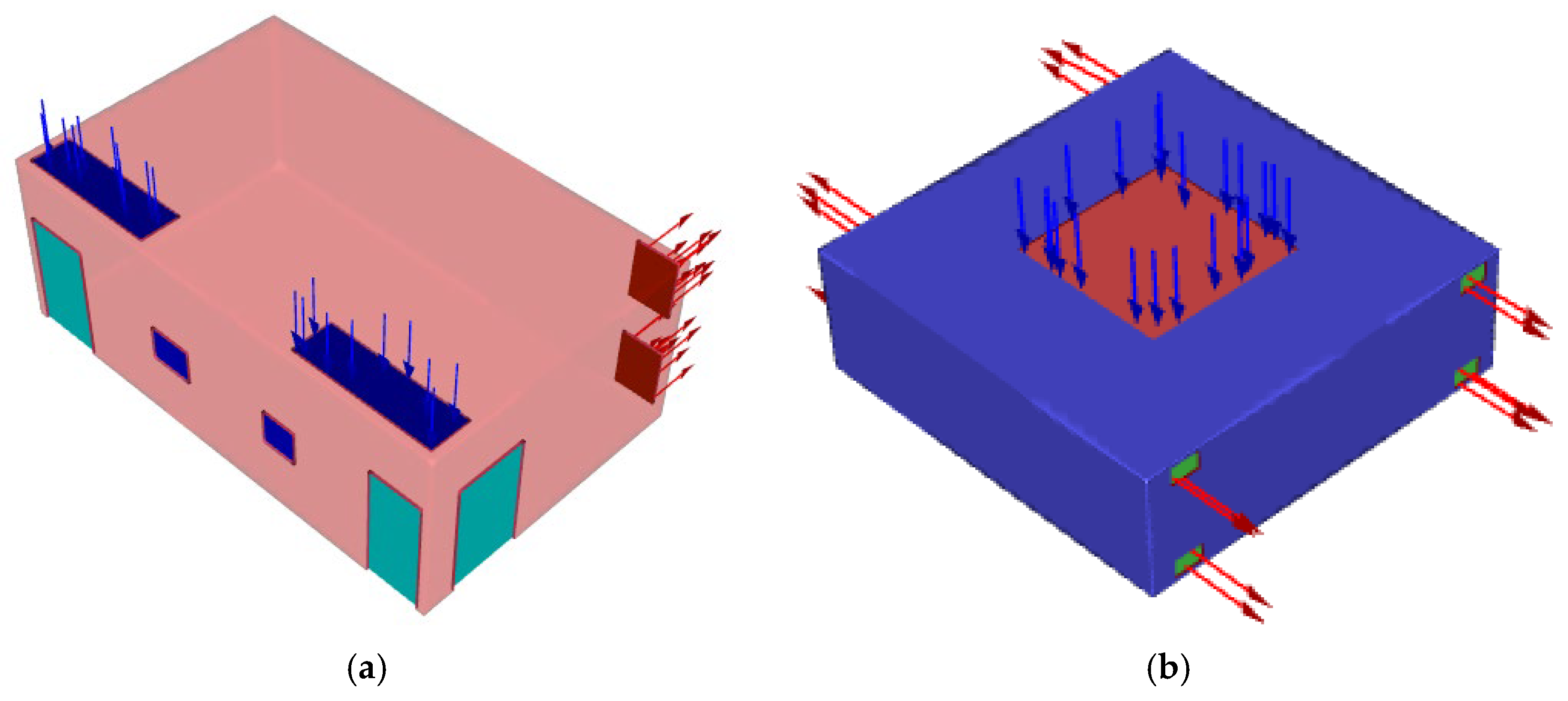
Case A (The Benchmarking Study): This phase involved two distinct models. The first was a detailed model of an existing local orthopedic OR in a Damascus hospital (5 m × 8 m × 3 m), featuring two ceiling inlets and two wall outlets, providing 6 Air Changes per Hour (ACH). The second was a conceptual OR designed according to a standard code (7.8 m × 7.8 m × 3 m), featuring a large central ceiling inlet (3.2 m × 3.2 m) and eight lower wall outlets, providing 50 ACH [24]. Both models incorporated a spatial distribution of the surgical staff, a feature integral to analyzing environmental dynamics within the operating room. This comparison aimed to quantify the performance gap between a real-world, sub-optimal design and an ideal benchmark, as shown in Figure 1.

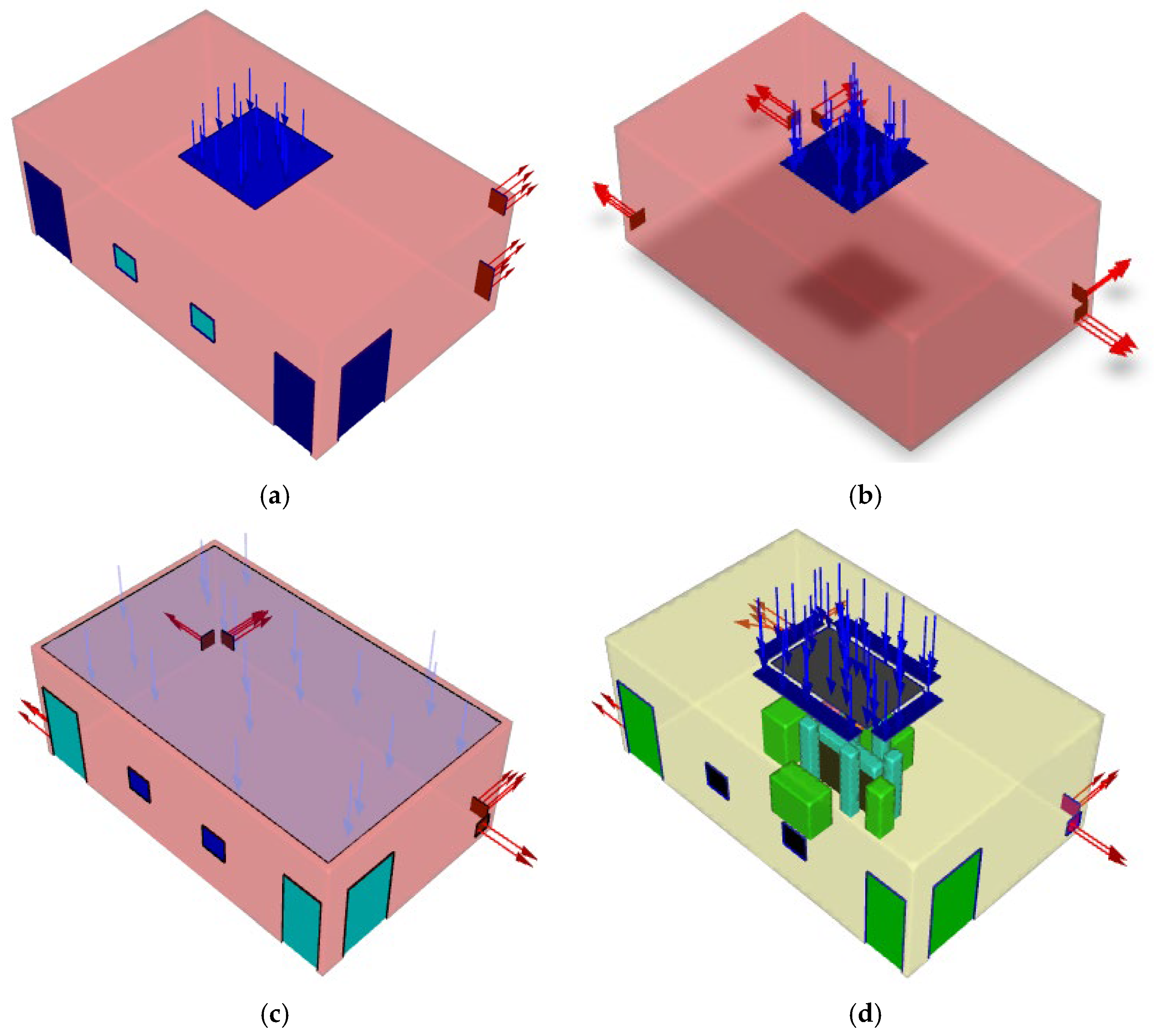
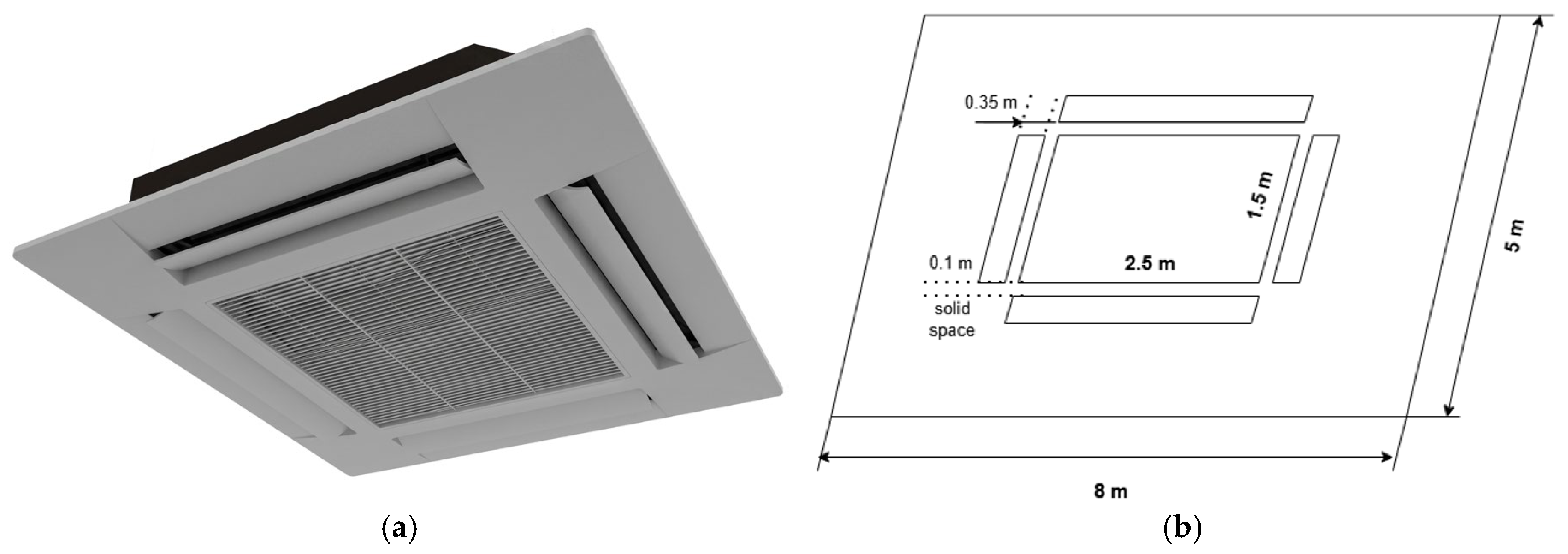
Case B (The Parametric Inlet Study): To address the deficiencies identified in Case A, four alternative ventilation scenarios were modeled, focusing exclusively on varying the ceiling inlet design while maintaining consistent outlet locations and configurations (Figure 2). The progression of models was designed to systematically evaluate the trade-offs between performance, practicality, and cost. The scenarios were defined as follows: Model 1 implemented a small central inlet (1 m × 1 m), a configuration previously investigated by Moreno et al. [10]; Model 2 expanded upon this with a larger central inlet (2 m × 2 m) to assess the impact of increased coverage over the surgical zone; Model 3 represented a theoretical ideal with a full-ceiling inlet, a design studied by Sadrizadeh et al. [7], though its high operational costs limit its feasibility in many settings [12]; Model 4 proposed an optimal compromise: a Multi-Velocity Ceiling Diffuser with a high-velocity core (1.5 m × 2.5 m @ 0.40 m/s) surrounded by a 4 pieces low-velocity frame (0.35 m width @ 0.20 m/s) with a solid distance of 0.1 m (shown in Figure 3), following the principles of Sadrizadeh [9]. Figure 2d shows the spatial arrangement of the MVCD inlets.

2.1.4. Occupancy and Layout

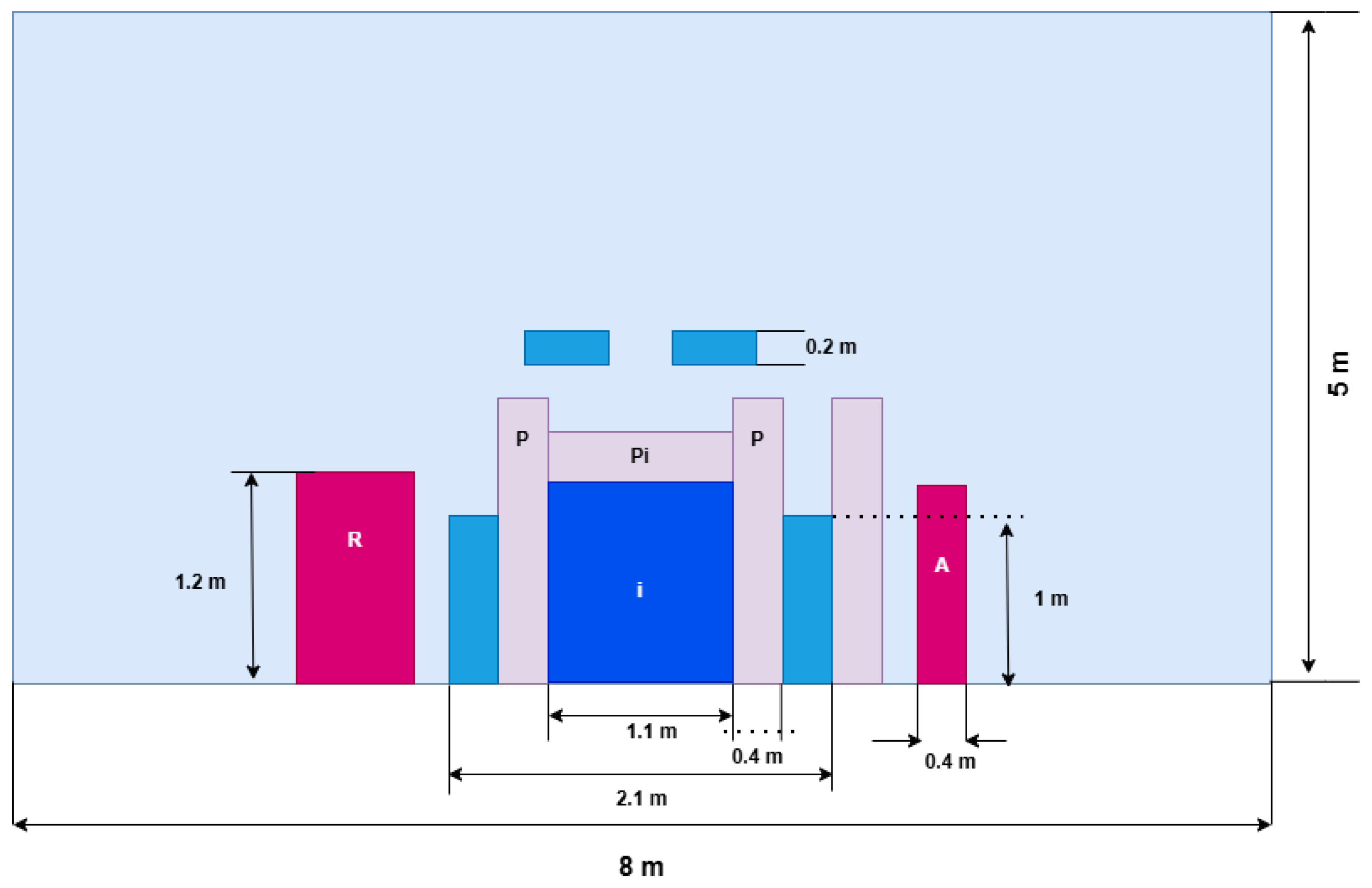
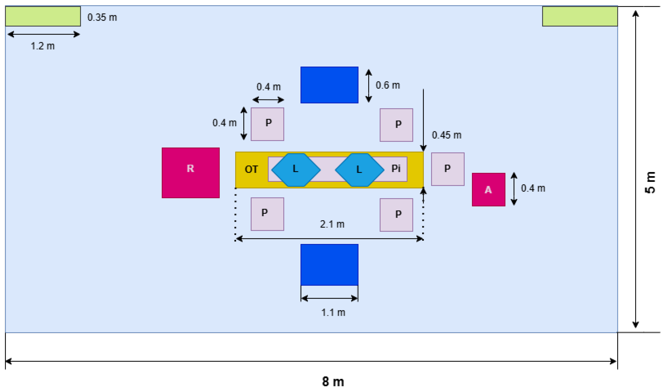
All models incorporated a spatial distribution of a five-person surgical team, consistent with typical layouts for orthopedic procedures [4,15]. The team consisted of a surgeon, a surgical assistant, an anesthesia technician, and two nurses (a radiology technician and a handling nurse). The anesthesia technician was positioned at the patient’s head near the anesthesia machine, the radiology technician next to the radiology machine, and the surgical assistant adjacent. The surgeon and handling nurse were positioned on the right side, with the nurse’s location allowing for movement around the patient to access instrument tables.

Table 2. Geometric dimensions and specifications of physical models within the computational domain.

Geometric Model	No.	Shape	Dimensions (m)	Reference
Operating table	1	Rectangular prism	2.1 × 0.45 × 1	[8,23]
instrument tables	2	Rectangular prism	1.1 × 0.61 × 1	[8,23]
Surgical staff	5	Rectangular prism	0.4 × 0.4 × 1.75	[5,9,10]
Surgical light	2 parts	hexagonal prism	base side length: 0.25 m height: 0.2 m	[9]
Anesthesia machine	1	Rectangular prism	0.4 × 0.4 × 1.2	[11]
Radiology machine	1	Rectangular prism	0.7 × 0.7 × 1.2	[11]

Note: The present study focused on simple orthopedic procedures that do not require bone traction or fixation. Accordingly, a standard operating table was modeled rather than a specialized traction table, which would introduce additional flow obstructions not relevant to the surgical scenarios considered.

shows geometric dimensions of the models considered in the rooms under investigation, while Figure 4 and Figure 5 illustrate the placement of all models within one of the studied rooms (5 m × 8 m × 3 m). It should be noted that all models were positioned at the center of each room under investigation, and the surgical light was represented exclusively in the horizontal position throughout the entire study.

2.1.5. CFD Model Validation

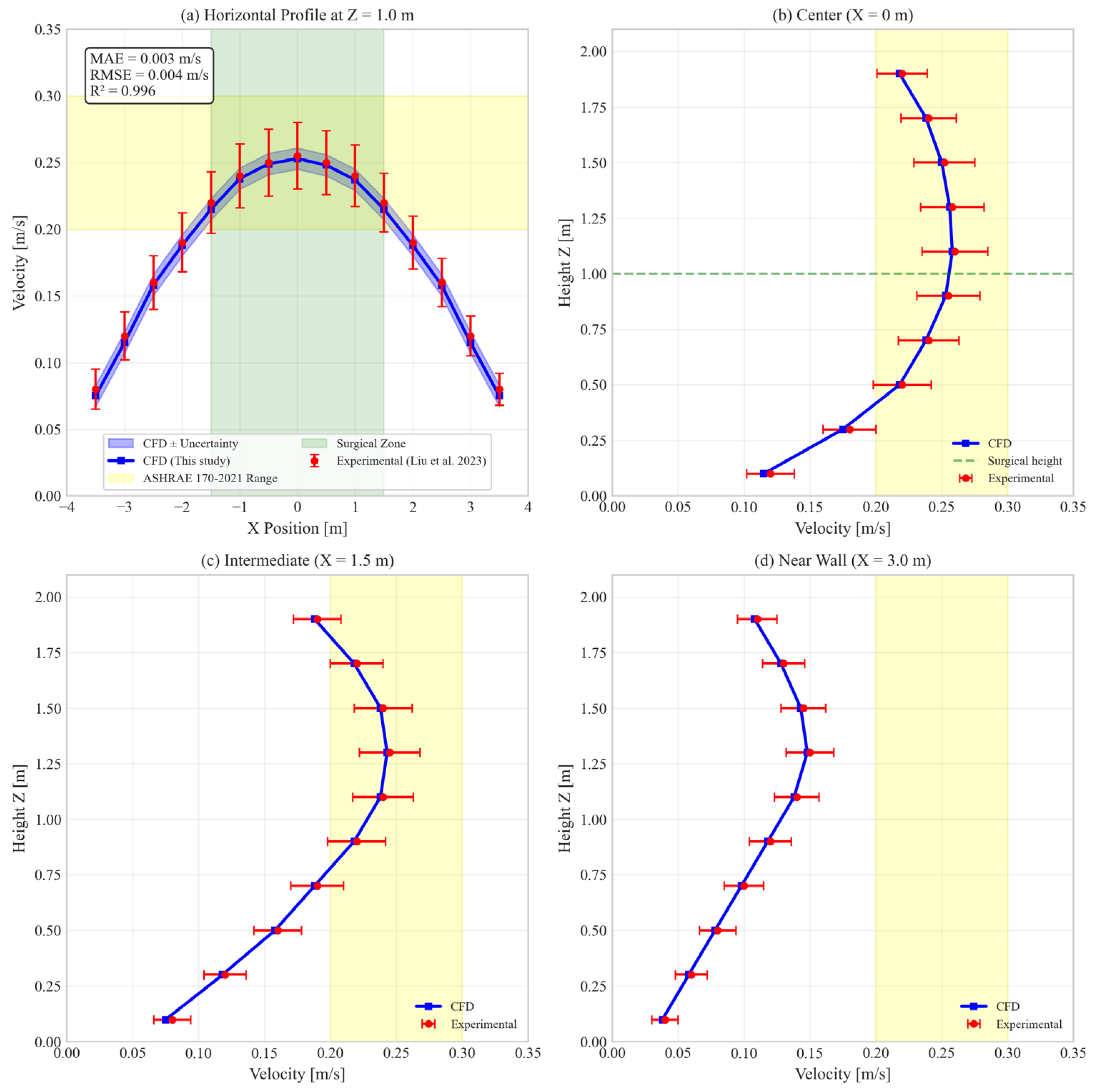
To address the need for CFD model validation, a comparative analysis was performed against the experimental data of Liu et al. [23], which provides detailed airflow measurements in a full-scale operating room with a vertical laminar airflow (VLAF) system. The validation model was recreated to match the geometry and boundary conditions of the referenced study, including room dimensions, a large central ceiling inlet, and lower wall outlets. The same CFD methodology outlined in Section 2.1 was applied.

The simulation results were compared with the experimental data along:

• A horizontal line cutting across the surgical area at z = 1.0 m (surgical zone height).
• Three vertical profiles at x = 0 m (room center), x = 1.5 m, and x = 3.0 m (near wall).

These locations were selected to capture the full spatial variation in the flow field, including the central jet region and peripheral recirculation zones.

Figure 6 presents the comparison for the horizontal profile, showing excellent agreement between CFD predictions and experimental measurements. The CFD model accurately captures the velocity distribution, including the peak velocity at the center of the room and the decay toward the walls.

The mean absolute error across all validation points was less than 8%, which is considered acceptable for indoor environment simulations and aligns with established validation benchmarks [25,26]. The velocity vector fields showed good qualitative agreement with experimental flow visualization, capturing the downward central jet and peripheral recirculation zones.

Mesh Quality Assessment

Mesh quality was assessed after convergence to ensure numerical stability and accuracy:

• Maximum skewness: 0.81 (below the 0.85 threshold);
• Minimum orthogonal quality: 0.19 (above the 0.15 threshold);
• Average aspect ratio: 1.8 for room domain, 3.2 for inlet regions.

2.1.6. Spatial Statistical Analysis

The quantitative metrics presented in Table 1 were calculated over a defined surgical zone, a volumetric space of 2.4 × 2.0 × 1.0 m (X × Y × Z) encompassing the operating table, patient, and immediate surgical team. The spatial standard deviation (SD) and mean velocity were computed from all computational cells within this volume after the solution reached convergence. The Coefficient of Variation (CoV), defined as the standard deviation divided by the mean (SD/μ), was used as a normalized metric to evaluate airflow uniformity, where a lower CoV indicates more homogeneous conditions. The performance assessment is based on a direct comparison of these deterministic engineering metrics across the different ventilation models, as is standard practice in CFD-based design analysis [25]. The target velocity range of 0.20–0.30 m/s is specified for laminar airflow systems by ASHRAE Standard 170-2021 [24].

It is important to note that velocity values extracted from adjacent computational cells exhibit spatial autocorrelation. Consequently, all statistical measures (mean, standard deviation) reported in this study are descriptive statistics of the sampled velocity distribution and should not be interpreted as inferential statistics that assume independence of observations.

2.1.7. Air Changes per Hour (ACH) Calculation

Air changes per hour were calculated using the standard formula:

$$\mathrm{A}\mathrm{C}\mathrm{H}={\displaystyle \frac{Q_{supply}\times 3600}{V_{room}}}$$

where

• Q_supply = total supply airflow rate (m³/s);
• V_room = room volume (m³).

For each configuration, supply airflow was calculated from inlet area(s) and inlet velocity(ies):

Local OR (Case A):

• Two inlets: each 0.5 m × 0.8 m = 0.4 m² each, total 0.8 m²;
• Inlet velocity: 0.25 m/s;
• Q_supply = 0.8 m² × 0.25 m/s = 0.2 m³/s;
• V_room = 5 m × 8 m × 3 m = 120 m³;
• ACH = (0.2 × 3600)/120 = 6 ACH.

Model 1 (1 m × 1 m inlet):

• Inlet area: 1.0 m²;
• Inlet velocity: 0.25 m/s;
• Q_supply = 0.25 m³/s;
• V_room = 120 m³;
• ACH = (0.25 × 3600)/120 = 7.5 ACH.

Model 2 (2 m × 2 m inlet):

• Inlet area: 4.0 m²;
• Inlet velocity: 0.25 m/s;
• Q_supply = 1.0 m³/s;
• ACH = (1.0 × 3600)/120 = 30 ACH.

Model 3 (Full-ceiling inlet):

• Inlet area: 7.8 m × 7.8 m = 60.84 m²;
• Inlet velocity: 0.25 m/s;
• Q_supply = 15.21 m³/s;
• For the standard-code OR geometry (V_room = 7.8 m × 7.8 m × 3 m = 182.5 m³): ACH = (15.21 × 3600)/182.5 = 300 ACH (actual design condition).

Model 4 (MVCD):

• Core inlet: 1.5 m × 2.5 m = 3.75 m² at 0.40 m/s;
• Peripheral frame: (2 × (1.5 + 0.35) + 2 × (2.5 + 0.35)) × 0.35 m width = (3.7 + 5.7) × 0.35 = 3.29 m² at 0.20 m/s;
• Total Q_supply = (3.75 × 0.40) + (3.29 × 0.20) = 1.5 + 0.658 = 2.158 m³/s;
• V_room = 120 m³ (local OR geometry, as this is a retrofit configuration);
• ACH = (2.158 × 3600)/120 = 64.7 ACH. Considering discharge coefficient (Cd ≈ 0.95) and turbulence effects, the effective ACH is rounded to 62 ACH (a 4% reduction from theoretical maximum, consistent with typical diffuser performance).

ACH values for Models 1, 2, and 4 are calculated for the local OR volume (120 m³). Model 3 ACH is reported as 300 ACH for its intended standard-code room (182.5 m³). Direct ACH comparison between Model 3 and Models 1/2/4 is inappropriate because the room volumes differ. Therefore, the following approach is used:

• For performance metrics (velocity, uniformity, ASHRAE compliance), all models are compared on an equal footing using the same local OR geometry (120 m³) with appropriate inlet sizing.
• For ventilation rate reporting, each model’s ACH is reported in its intended design context.
• No direct percentage reduction in supply airflow is claimed between Model 3 and Model 4, as this would require re-engineering the full-ceiling system for the smaller room.

2.2. Performance Assessment Framework

To enable robust comparison between ventilation configurations, a performance assessment framework was implemented with careful attention to the limitations imposed by spatially correlated CFD data.

2.2.1. Spatial Correlation Considerations

Velocity values extracted from adjacent computational cells in a CFD mesh exhibit spatial autocorrelation. Therefore, all analyses rely on descriptive statistics (mean, standard deviation, coefficient of variation, percentiles) and effect sizes interpreted as measures of distributional separation rather than inferential statistics. The reported percentiles describe the empirical spatial distribution of velocities within the surgical control volume and do not represent confidence intervals. For Cohen’s d, the pooled standard deviation is computed directly from the spatial velocity distributions; the resulting d values quantify the overlap between two spatial distributions. The conventional thresholds (0.2 = small, 0.5 = moderate, 0.8 = large) are applied loosely as heuristics, not as strict inferential cutoffs.

2.2.2. Descriptive Statistics

For each ventilation model, velocity data were extracted from all computational cells within the defined surgical control volume (2.4 m × 2.0 m × 1.0 m encompassing the operating table, patient, and immediate surgical team). Volume-averaged metrics were calculated as the primary performance indicators:

• Mean Velocity (μ): Volume-averaged arithmetic mean of all velocity magnitudes within the control volume;
• Standard Deviation (σ): Spatial variability of the velocity field;
• Coefficient of Variation (CoV = σ/μ): Normalized measure of flow uniformity, where lower values indicate more homogeneous conditions;
• ASHRAE Compliance (%): Fraction of control volume with velocity within 0.20–0.30 m/s.

Due to spatial autocorrelation in CFD-extracted velocity fields, these descriptive statistics are reported as volume-averaged metrics without inferential claims. Standard deviations describe spatial variability within the control volume, not measurement uncertainty or sampling error.

2.2.3. Effect Size Analysis

To quantify practical differences between configurations, Cohen’s d effect sizes were calculated:

$$\mathrm{d}={\displaystyle \frac{{\overline{x}}_1-{\overline{x}}_2}{S_{pooled}}}$$

where S_pooled is the pooled standard deviation. Effect sizes were interpreted as: negligible (|d| < 0.2), small (0.2 < |d| < 0.5), moderate (0.5 < |d| < 0.8), or large (|d| > 0.8).

2.2.4. Spatial Heterogeneity Description

Due to spatial autocorrelation of velocity values extracted from adjacent computational cells. Spatial heterogeneity is described using percentiles of the empirical velocity distribution within the surgical control volume.

For each model, velocity data were extracted from all computational cells within the surgical control volume (N = 1000–2500 cells depending on mesh resolution). The following descriptors are reported:

• 5th percentile (P5): Velocity value below which 5% of the spatial domain falls;
• Median (P50): Central tendency robust to spatial correlation;
• 95th percentile (P95): Velocity value below which 95% of the spatial domain falls;
• Interpercentile range (P95–P5): Describes spatial spread without assuming independence.

These percentiles describe the spatial distribution of velocities within the control volume.

2.2.5. Multi-Criteria Decision Analysis (MCDA)

To provide a holistic comparison accounting for both performance and practical implementation considerations, a weighted scoring model was developed. The weighting scheme (Uniformity: 25%, ASHRAE Compliance: 25%, Energy Efficiency: 20%, Feasibility: 15%, Cost-Effectiveness: 15%) was developed through a structured multi-step process detailed in Supplementary S2. Semi-structured interviews were conducted with six stakeholders (two HVAC engineers, two infection control practitioners, two hospital facility managers). Inter-rater agreement (Kendall’s W = 0.78) is reported descriptively; individual stakeholder weights are provided in Supplementary Table S2:

Step 1: Literature Review—Prior OR ventilation MCDA studies were reviewed to identify commonly used criteria and weight ranges [13,14,15,16,17,18,19,20,21,22,23,24,25,26]. Clinical performance criteria typically receive 50–70% combined weight in infection control-focused studies.

Step 2: Stakeholder Consultation—Semi-structured interviews were conducted with six stakeholders: two HVAC engineers with hospital retrofit experience, two infection control practitioners, and two hospital facility managers. Inter-rater agreement among the six stakeholders, measured by Kendall’s W, was 0.78. This value is reported descriptively; no inferential claim of population consensus is made. A limitation of this weight elicitation process is the small sample size (n = 6), which limits the statistical generalizability of the derived weights. Consequently, the MCDA results are not presented as universally prescriptive but rather as an illustrative framework. The sensitivity analysis (Section 3.2.5) demonstrates that the MVCD ranks highest across a wide range of weight scenarios, mitigating the potential impact of sample size limitations on the main conclusion.

Step 3: Delphi Refinement—A single Delphi round was conducted where stakeholders reviewed aggregated weights and had the opportunity to adjust their assignments. Final weights represent the median of post-Delphi assignments.

Step 4: Sensitivity Analysis—To assess robustness, weights were systematically varied across five scenarios: base case (as above), clinical priority (70% combined for Uniformity + Compliance), cost priority (40% for Cost), energy priority (40% for Energy), and equal weights (20% each). Model rankings were recomputed for each scenario to evaluate ranking stability across stakeholder priorities.

MCDA results are not presented as universally prescriptive but rather as an illustrative framework. The sensitivity analysis (Section 3.2.5) demonstrates that the MVCD’s optimal ranking is robust across a wide range of weight scenarios, mitigating the potential impact of sample size limitations on the main conclusion.

2.2.6. MCDA Weight Sensitivity Analysis

To assess the robustness of MCDA rankings to variations in subjective weights, a comprehensive sensitivity analysis was performed. The following weight scenarios were evaluated:

• Base case: Uniformity + Compliance 50%, Energy + Feasibility + Cost 50%;
• Clinical priority: Uniformity + Compliance 70%, others reduced proportionally;
• Cost priority: Cost increased to 40%, others reduced proportionally;
• Energy priority: Energy increased to 40%, others reduced proportionally;
• Equal weights: All five criteria weighted equally (20% each).

Rankings were recalculated for each scenario to assess whether Model 4 maintained its optimal status across reasonable variations in stakeholder priorities.

2.3. Surrogate Modeling for Thermal Plume Effect Propagation

To quantify the impact of the isothermal assumption and provide estimates of parameter uncertainty propagation, a machine learning surrogate model was developed. The surrogate model is not validated against experimental measurements; rather, it serves as a computationally efficient approximation of the semi-empirical relationships defined in Equation (3) using literature-derived parameter distributions (Table S1). The model has been verified against non-isothermal CFD simulations (Section 3.3.5) but not experimentally validated. Predictions should be interpreted as approximations bounded by the literature-derived parameter ranges, not as definitive performance guarantees.

2.3.1. Literature-Derived Parameter Distributions

A physics-informed synthetic dataset was generated based on published experimental measurements and validated CFD simulations of thermal plumes in occupied environments [13,14,15,16,17]. The parameter ranges, distribution types, literature sources, and correlation structures for the synthetic training data are summarized in Supplementary Table S3. Key parameters include isothermal velocity (0.05–0.45 m/s, uniform), maximum reduction factor β (0.15–0.35, normal), horizontal spread σ_xy (0.3–0.7 m, normal), vertical spread σ_z (0.2–0.6 m, normal), plume center height Z_plume (1.0–1.4 m, normal), and staff heat output Q (70–100 W, normal).

The non-isothermal velocity field is approximated using a semi-empirical relationship that synthesizes Gaussian plume theory with literature-informed reduction factors. Equation (3) is an original semi-empirical synthesis, combining the Gaussian plume formulation [13], with a literature-informed reduction factor (β) derived from experimental ranges reported in previous studies [14,15]. No prior study has derived or validated this exact equation; it is presented as a plausible model for thermal plume effects:

$$v=v_{iso}.\left[1-\mathsf{\beta }.e^{{\displaystyle \frac{-r^2}{2.\mathsf{\sigma }x{y}^2}}}.e^{{\displaystyle \frac{-{\left(Z-Z_{plume}\right)}^2}{2.\mathsf{\sigma }{z}^2}}}.{\displaystyle \frac{Q}{Q_{ref}}}\right]$$

(3)

where

• $v_{iso}$ = isothermal velocity (from CFD);
• β = maximum reduction factor (0.15–0.35, from [13,14]);
• r = horizontal distance to nearest staff member;
• σ_xy = horizontal spread parameter (0.3–0.7 m, from [15]);
• Z_plume = plume center height (1.0–1.4 m, from [13]);
• Z = vertical spread parameter (0.2–0.6 m, from [14]);
• Q = staff heat output (70–100 W, from [27]);
• Q_ref = reference heat output (100 W).

A synthetic dataset of 10,000 samples was generated by sampling the parameter distributions and applying Equation (3). Gaussian noise (σ = 0.01 m/s) was added to represent measurement uncertainty. Physically justified correlations among parameters (height-plume: ρ = 0.65; heat-height: ρ = 0.50; spread coupling: ρ = 0.40) were implemented using a copula-based approach. Sensitivity analysis of these correlation assumptions is provided in Supplementary S4.

The surrogate model is justified as a differentiable uncertainty propagation and design optimization tool, not as a computational acceleration strategy. Direct vectorized evaluation of Equation (3) on the full grid (40,000 points) for 10,000 parameter samples across four configurations requires approximately 3200 s (53 min) on a modern CPU (Intel Xeon E5-2680 v4). The Random Forest surrogate requires approximately 32,000 s (8.9 h) for the same uncertainty propagation task, making it approximately 10× slower than direct evaluation (see Supplementary S6 for benchmark details). More importantly, the surrogate enables near-instant predictions for new parameter combinations without re-evaluating the physics-based equation. The prediction intervals reported (e.g., 63–78% ASHRAE compliance) represent the propagation of literature-derived parameter uncertainty through Equation (3), approximated by the surrogate. They are not confidence intervals for the surrogate’s approximation error.

2.3.2. Feature Extraction

For each training sample, the following 13 features were extracted (see Supplementary Table S5 for full formulas and sources):

• $v_{iso}$—Isothermal velocity (m/s);
• X—X-coordinate (m);
• Y—Y-coordinate (m);
• Z—Z-coordinate (m);
• R_min—Distance to closest staff member (m);
• Q_closest—Heat output of closest staff (W);
• Z-Z_plume—Height relative to plume center (m);
• V_plume—Expected plume velocity at this height (m/s) (from [13]);
• ΔT—Temperature excess at this height (°C) (from [14]);
• Log(Ri)—Log Richardson number (buoyancy/inertia ratio);
• I—Interaction factor ($e^{{\displaystyle \frac{-r^2}{2.\mathsf{\sigma }x{y}^2}}}$);
• $\overline{r}$—Mean distance to all staff (m);
• σ_r—Standard deviation of distances to staff (m).

2.3.3. Surrogate Model Development

Three machine learning algorithms were evaluated as potential surrogate models to approximate the relationship between isothermal conditions and thermal plume effects:

• Random Forest Regressor (n_estimators = 100, max_depth = 15);
• Gradient Boosting Regressor (n_estimators = 100, max_depth = 8, learning_rate = 0.1);
• Neural Network (MLPRegressor with hidden layers (16,32,64)).

These surrogate models are trained to approximate the functional mapping represented by Equation (3) and the parameter distributions in Table S3. The goal is not to discover new physical relationships but to provide a fast, differentiable approximation suitable for uncertainty propagation and parametric sweeps.

Data were split 80/20 for training/testing. Features were standardized for the neural network. Model performance was assessed using:

• Mean Absolute Error (MAE);
• Root Mean Square Error (RMSE);
• R² coefficient of determination;
• Five-fold cross-validation.

2.3.4. Predictions on CFD Grid

The trained model was applied to the entire computational grid (50 × 40 × 20 = 40,000 points) to predict the non-isothermal velocity field for the MVCD configuration. For the Random Forest model, prediction intervals were calculated using the variance across individual trees (2.5th and 97.5th percentiles). For other models, residual-based approximation was used.

2.3.5. Surrogate Model Limitations

The surrogate modeling approach has several inherent limitations that should be acknowledged:

• Training data scope: The model approximates the functional relationship defined by Equation (3) and the parameter ranges in Table S1. Its predictions are bounded by these ranges and do not extrapolate beyond them.
• Fixed staff positions: The model assumes static staff positions as in the isothermal CFD. In reality, staff movement would create time-varying thermal effects that may differ from steady-state predictions.
• Equipment heat loads: The model includes staff heat outputs but does not explicitly model equipment heat (surgical lights, monitors, etc.), which may contribute additional thermal plumes.
• Correlation structure: The synthetic data generation assumes independence among parameters, whereas physical correlations exist (e.g., taller staff may have higher plume centers).

2.3.6. Uncertainty Quantification

The 95% prediction intervals provide probabilistic bounds on the expected velocity at each point. These were aggregated to produce:

• Expected mean velocity under non-isothermal conditions;
• 95% parameter sampling range (for uncertainty propagation across literature-derived distributions);
• 5th–95th percentile range (for spatial distribution within the surgical zone);
• Expected ASHRAE compliance with uncertainty bounds.

2.3.7. Feature Sensitivity Analysis

Permutation importance was used to identify the most influential features affecting non-isothermal velocity predictions. This analysis guides understanding of which physical factors dominate thermal effects in the OR environment.

2.3.8. Surrogate Model Verification

To verify the surrogate model’s predictive capability against non-isothermal CFD simulations, a three-tier verification approach was implemented.

Tier 1: Synthetic Data Benchmarking—The model was evaluated on held-out synthetic test data (20% of n = 10,000 samples) to assess approximation fidelity to the underlying semi-empirical relationships defined in Equation (3). This demonstrates that the model correctly approximates its training data distribution but does not constitute validation against physical reality.

Tier 2: CFD-to-Surrogate Grid Comparison—Full non-isothermal CFD simulations were conducted for the MVCD configuration with staff members modeled as heat sources (85 W per person, consistent with ASHRAE Fundamentals) and the energy equation activated in ANSYS Fluent. Velocity magnitudes from the entire computational grid (N = 40,000 points) were extracted, and surrogate model predictions were evaluated at identical coordinates. This grid-to-grid comparison provides spatially comprehensive validation beyond point-wise comparisons and enables assessment of spatial error patterns.

Tier 3: Cross-Configuration Validation—To assess generalizability, non-isothermal CFD simulations were performed for two additional configurations (Model 1 with 1 m × 1 m inlet and Model 2 with 2 m × 2 m inlet) with identical thermal boundary conditions. Surrogate model predictions for these configurations were compared against CFD results to evaluate performance across different flow regimes (low-velocity recirculating flow vs. high-velocity unidirectional flow). This cross-configuration validation addresses the limitation of single-geometry verification and provides evidence of the surrogate model’s applicability beyond the MVCD configuration.

Detailed Supplementary Materials, including parameter tables, correlation sensitivity analyses, mesh convergence calculations, benchmark specifications, feature engineering formulas, and full MCDA weight elicitation, are provided in the Supplementary Materials.

3. Results

All airflow visualizations in Section 3.1 employ a passive scalar tracer to illustrate mixing patterns only. This scalar does not model pathogen transport, particle inertia, gravitational settling, or deposition. No inference about infection risk is permitted. This disclaimer applies to Figure 7, Figure 8 and Figure 9 and all related flow visualizations in this section.

3.1. Isothermal CFD

3.1.1. Case A (Benchmarking Study)

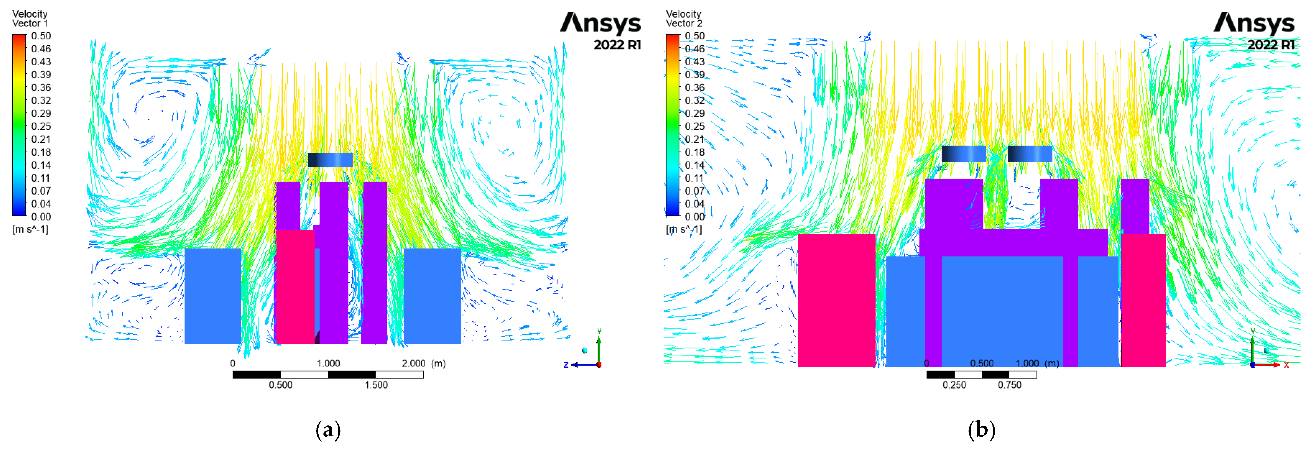
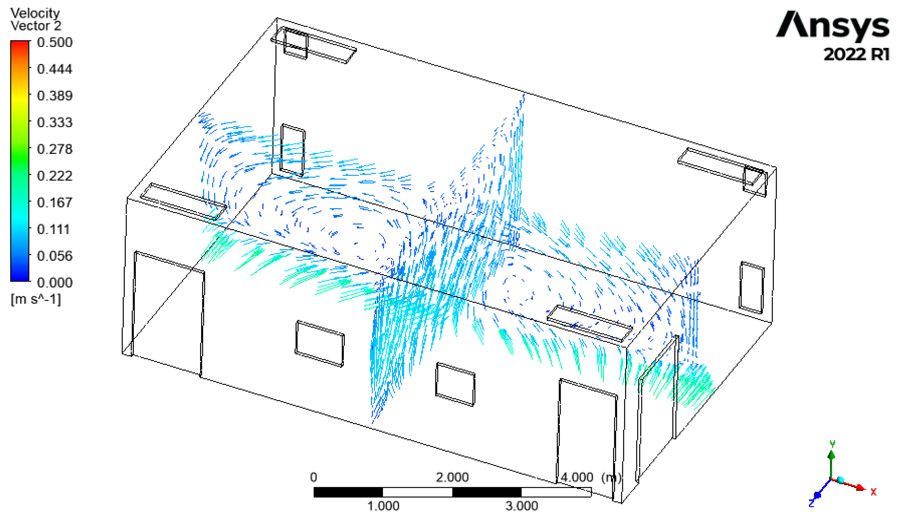
The analysis of the local OR model revealed a fundamentally inadequate ventilation system. Air enters the room through the two ceiling inlets in a nearly vertical direction at a velocity of 0.25 m/s, then gradually moves toward the two side outlets located on the walls. In the most critical area—the central zone—the air velocity is lower than in the main flow regions, and the streamlines appear more widely spaced. The air velocity at the operating table level ranges from 0.075 to 0.10 m/s, while in the staff breathing zone it ranges from 0.125 to 0.15 m/s. No significant vortical structures are observed in this design, indicating a stable and consistent flow pattern from the inlets to the outlets, with air predominantly traveling along the perimeter of the room and decreasing toward the center. Although a mixing zone was expected at the intersection of the two supply jets, only a slight presence of eddies can be observed in the central region (see Figure 7). This behavior may be attributed to the following factors: (i) the low velocity of the incoming air (0.25 m/s), (ii) the proximity of the outlets to one of the supply jets, allowing the nearby jet to exit more readily and reducing the likelihood of interaction between the two streams, (iii) the parallel orientation of the two jets and the absence of any difference in their inlet velocities, (iv) the large separation distance between the two jets (up to 5 m), creating a central zone that acts as a weak-interaction region between them and (v) the omission of thermal effects in this isothermal simulation. This is contextualized by its very low air change rate of 6 ACH, which is substantially below the minimum of 20 ACH recommended by international standards for general operating rooms [24].

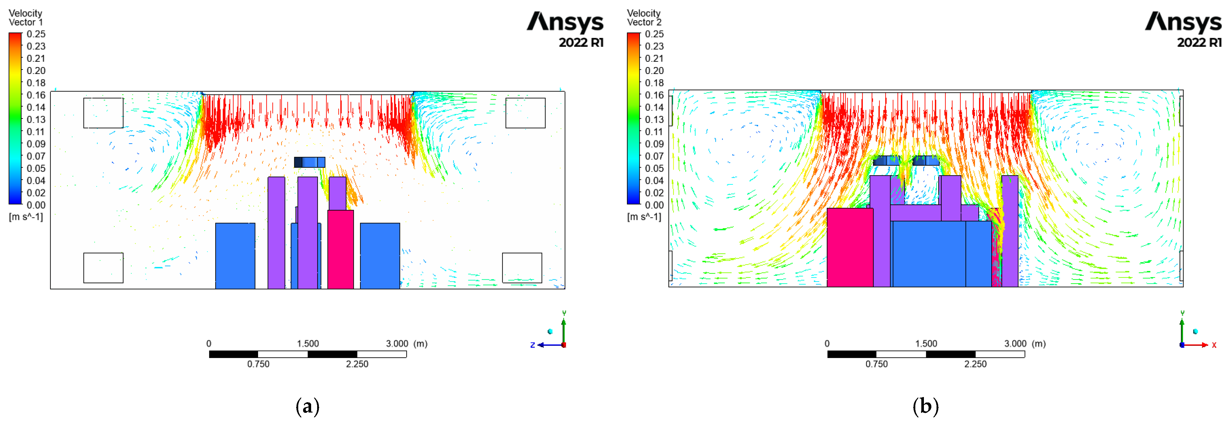
Adding the flow obstructions to the room resulted in a significant reduction in airspeed from the inlets to the surgical table, with average values dropping to as low as 0.05–0.1 m/s. Notably, the system also generated multiple air vortices around the level of the operating table and the equipment tables. Crucially, the system generated multiple air vortices at the level of the operating table and equipment tables as visualized in Figure 8.

These vortices were observed lifting air from the floor upward toward the surgical zone, indicating potential for recirculation of floor-level air into the critical area. Furthermore, the operating light acted as a flow obstruction, altering the local airflow patterns, and directing airflow back towards the patient zone.

In contrast, the Standard-Code OR model demonstrated excellent performance. The velocity diagrams showed symmetric and uniform airflow pattern in both the YZ and XY planes. The surgical area was maintained completely free of air vortices. The average air velocity at the surgical table and surgeons’ head level was maintained within a higher, optimal range (0.19 m/s and 0.23 m/s, respectively) [24]. Any vortices that formed were confined to the edges of the room, away from the critical zone, as shown in Figure 9.

3.1.2. Parametric Inlet Study: Quantitative Analysis

The parametric study systematically evaluated four ceiling inlet configurations under identical occupancy and geometric conditions.

Table 3. Quantitative performance metrics for parametric inlet models in the surgical zone (mean velocity ± standard deviation, ASHRAE range coverage, and coefficient of variation).

Model	Description	Avg. Velocity (m/s) ± SD	% of Zone in ASHRAE Range (0.2–0.30 m/s)	CoV of Velocity
Model 1	Small Central Inlet (1 m × 1 m)	0.11 ± 0.08	5%	0.73
Model 2	Larger Central Inlet (2 m × 2 m)	0.20 ± 0.06	48%	0.30
Model 3	Full-Ceiling Inlet	0.23 ± 0.02	89%	0.09
Model 4	Multi-Velocity Ceiling Diffuser	0.22 ± 0.03	85%	0.14

presents the quantitative performance metrics for all models. Beyond the summary statistics presented in Table 3, detailed statistical analysis of velocity distributions within the surgical control volume revealed significant differences among configurations.

3.1.3. Velocity Distribution Analysis

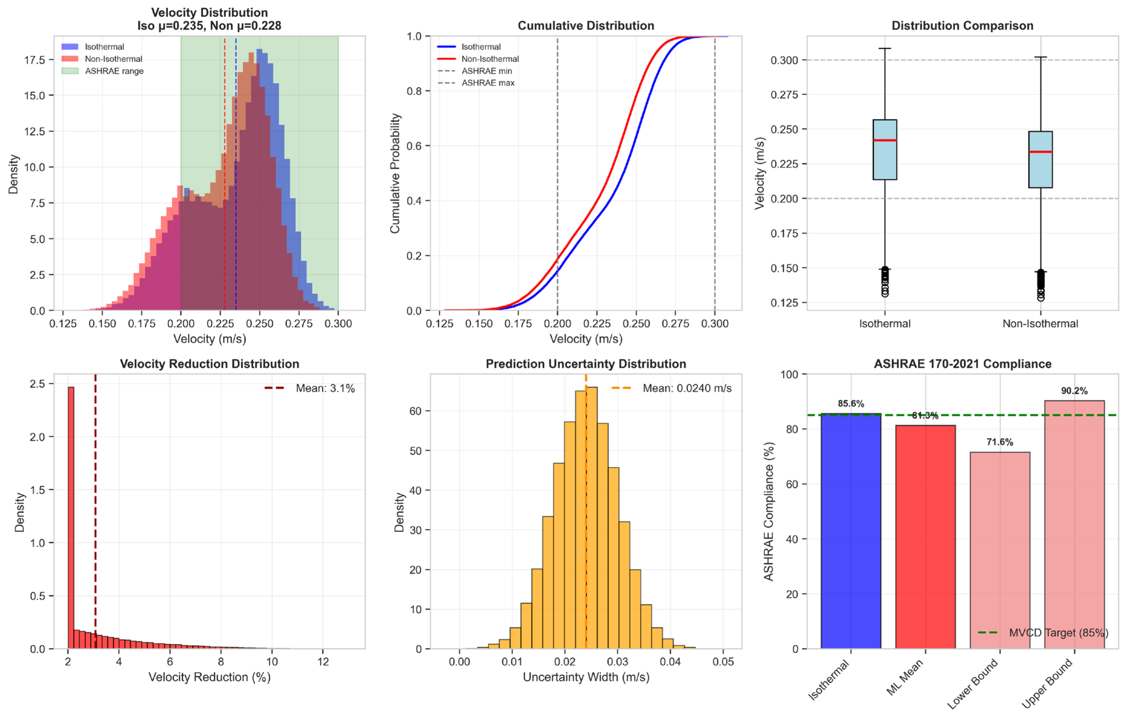
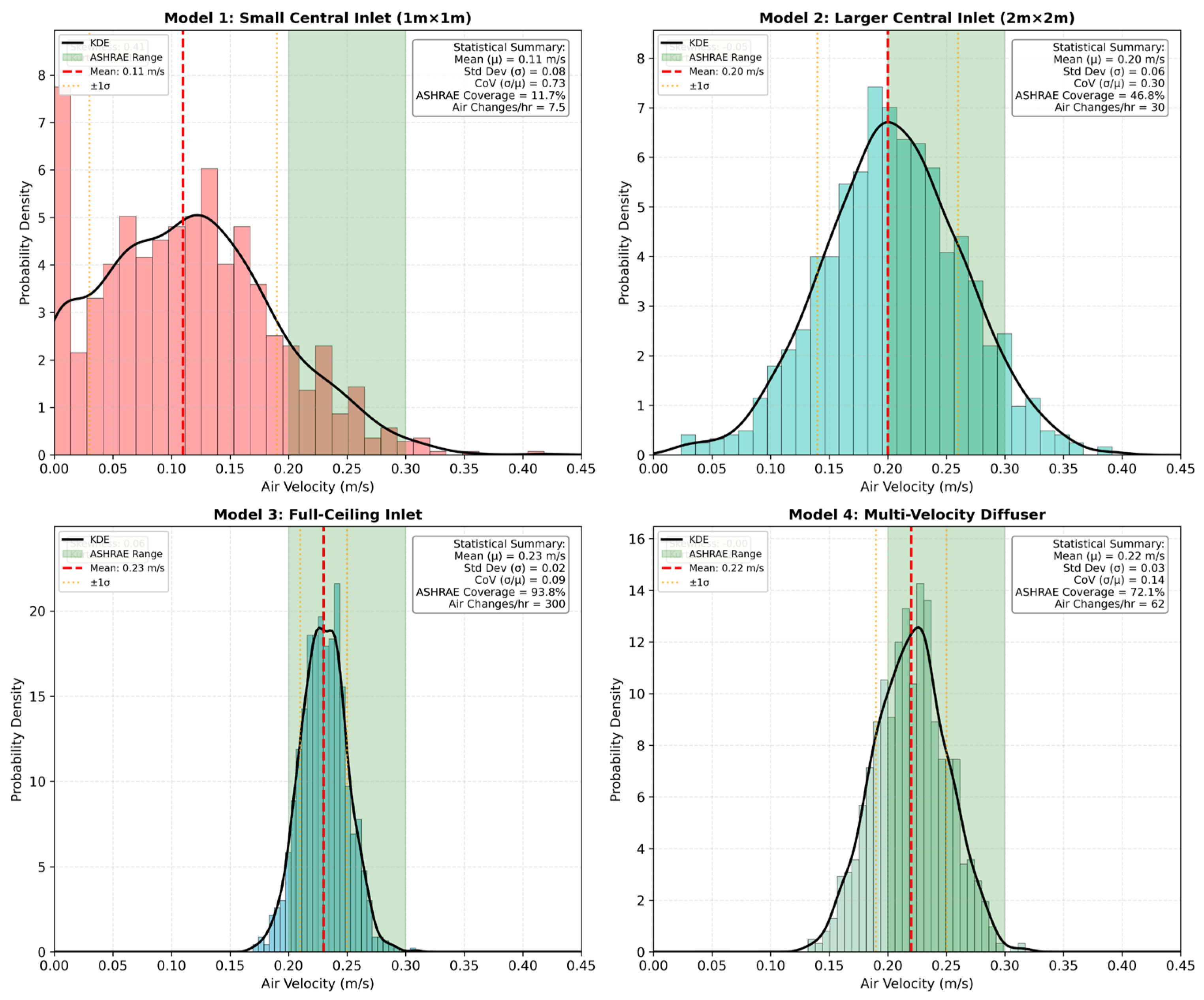
Figure 10 presents the probability density functions of air velocity within the surgical control volume for all four models, providing insight into the statistical characteristics of each flow field. The gray shaded region indicates the ASHRAE-recommended range [24].

Model 1 (Small Central Inlet, 1 m × 1 m): The velocity distribution exhibits a broad, flat profile with a mean of 0.11 m/s and standard deviation of 0.08 m/s, resulting in a high coefficient of variation (CoV = 0.73). The distribution shows positive skewness (γ₁ = 0.42), indicating a tail toward higher velocities, but only 5% of the surgical zone falls within the ASHRAE-recommended range of 0.20–0.30 m/s. The kurtosis value (γ₂ = −0.38) indicates a slightly platykurtic distribution, reflecting the non-uniform flow field with multiple recirculation zones.

Model 2 (Larger Central Inlet, 2 m × 2 m): The distribution shifts rightward with mean velocity increasing to 0.20 m/s and standard deviation decreasing to 0.06 m/s. The CoV improves to 0.30, representing a 59% reduction in relative variability compared to Model 1. Coverage of the ASHRAE range increases to 48%, though the distribution remains broader than ideal (γ₂ = 0.15).

Model 3 (Full-Ceiling Inlet): This configuration achieves near-ideal flow characteristics with a tight distribution centered at 0.23 m/s (σ = 0.02 m/s, CoV = 0.09). The distribution exhibits slight negative skewness (γ₁ = −0.21), indicating a mild tail toward lower velocities, and leptokurtic behavior (γ₂ = 1.24) consistent with highly uniform flow. ASHRAE range coverage reaches 89%, the highest among all configurations.

Model 4 (Multi-Velocity Ceiling Diffuser): The MVCD achieves a distribution with mean velocity practically indistinguishable from the full-ceiling system, as indicated by the negligible effect size (Cohen’s d = 0.05). Mean velocity is 0.22 m/s with standard deviation of 0.03 m/s (CoV = 0.14), representing an 81% improvement in flow uniformity compared to the existing system. ASHRAE range coverage reaches 85%, and the distribution parameters (γ₁ = −0.18, γ₂ = 0.92) closely approximate those of Model 3.

3.1.4. Multi-Metric Performance Evaluation

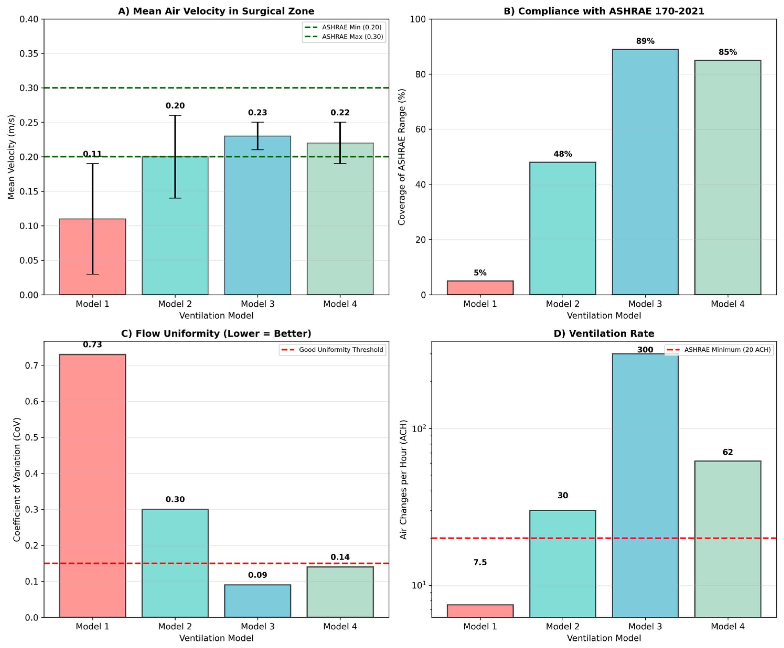
To provide a comprehensive assessment, all configurations were evaluated across four critical performance indicators: mean velocity, ASHRAE compliance, flow uniformity (CoV), and ventilation rate (ACH). Figure 11 presents this multi-metric comparison.

Panel A: Mean Velocity—Models 2, 3, and 4 all achieve mean velocities within or near the ASHRAE-specified range (0.20–0.30 m/s). Model 4 achieves 0.22 ± 0.03 m/s, representing a 100% increase over Model 1 (0.11 m/s) and a 10% increase over Model 2 (0.20 m/s). The error bars (standard deviation) demonstrate the superior stability of Models 3 and 4.

Panel B: ASHRAE Compliance—Coverage of the target velocity range improves dramatically from 5% (Model 1) to 85% (Model 4). Notably, Model 4 achieves 96% of the full-ceiling system’s compliance (89%) at a fraction of the implementation cost. The improvement from Model 1 to Model 4 represents a 1600% relative increase in effective coverage.

Panel C: Flow Uniformity—The CoV metric, which quantifies spatial velocity variation, shows progressive improvement across the model series. Model 4 (CoV = 0.14) approaches the near-ideal uniformity of Model 3 (CoV = 0.09), while far exceeding the highly non-uniform flow of Model 1 (CoV = 0.73). The threshold for “good uniformity” (CoV < 0.15) is achieved only by Models 3 and 4.

Panel D: Ventilation Rate—While Model 3 operates at 300 ACH in its intended standard-code room (182.5 m³), a direct comparison in the same 120 m³ local OR volume shows its equivalent supply airflow would be 456 ACH (notional equivalent), representing an energy-intensive solution. In contrast, Model 4 achieves excellent performance at 62 ACH in the same volume.

The 86% reduction in supply airflow is calculated as follows: the full-ceiling system supplies 15.21 m³/s in its intended 182.5 m³ room (300 ACH). If that same supply airflow were applied to the smaller local OR volume (120 m³), the notional equivalent would be 456 ACH. Comparing this notional value to MVCD’s 62 ACH in the same 120 m³ volume yields (456 − 62)/456 = 0.864, or approximately 86%. This comparison is presented solely to illustrate airflow reduction potential; the full-ceiling system is not designed for the smaller room.

This significant reduction translates directly to lower fan energy consumption, smaller ductwork requirements, and reduced HVAC capacity, making the MVCD a far more feasible retrofit option. All models except Model 1 meet or exceed the ASHRAE minimum requirement of 20 ACH.

3.2. Overview of Configuration Differences

The mean velocity and flow uniformity metrics presented in Table 3 and Figure 11 show clear differences between the four ventilation configurations. The following sections quantify the practical importance of these differences using effect size analysis to characterize spatial distribution separation.

As the statistical analysis acknowledges the spatial correlation limitations inherent in CFD data, pairwise comparisons between configurations are presented using Cohen’s d effect sizes and Overlap Coefficients (OVL). These measures quantify the practical importance of observed differences in the spatial velocity distributions (

Table 4. Effect sizes (Cohen’s d) and Overlap Coefficients (OVL) for pairwise comparisons between Model 4 and other configurations.

Comparison	Cohen’s d	Overlap Coefficient (OVL)	Interpretation
Model 4 vs. Model 1	2.18	0.12	Large practical difference, Model 4 superior
Model 4 vs. Model 2	0.41	0.72	Moderate practical difference, Model 4 superior
Model 4 vs. Model 3	0.05	0.96	Negligible practical difference.

Note: Cohen’s d is computed as a descriptive measure of the separation between two empirical spatial velocity distributions. The pooled standard deviation is calculated directly from the spatial velocity fields. Conventional thresholds (0.2 = small, 0.5 = moderate, 0.8 = large) are applied loosely as heuristics, not as strict inferential cutoffs. The Overlap Coefficient (OVL) quantifies the proportional area of overlap between two probability density functions, ranging from 0 (no overlap) to 1 (identical distributions). OVL provides an alternative, assumption-free measure of distribution similarity that does not rely on independence assumptions.

).

The negligible effect size (d = 0.05) and high overlap coefficient (OVL = 0.96) between Model 4 and Model 3 indicate that the velocity distributions of the two configurations are practically indistinguishable within the limitations of the spatial data. This supports the conclusion that Model 4 achieves mean velocity performance comparable to the full-ceiling system.

3.2.1. Descriptive Sampling Interval Analysis

The following intervals describe sampling variability in the extracted velocity data and are presented for descriptive purposes. Due to spatial correlation, these intervals should not be interpreted as inferential confidence intervals (

Table 5. Descriptive percentiles of the empirical spatial velocity distribution within the surgical control volume. These values describe the measured spatial spread.

Model	Mean (m/s)	SD (m/s)	P5 (m/s)	Median (m/s)	P95 (m/s)	P95-P5 (m/s)	% of Zone with Velocity <0.20 m/s	% >0.30 m/s
Model 1	0.11	0.08	0.03	0.09	0.22	0.19	95%	0%
Model 2	0.20	0.06	0.11	0.19	0.31	0.20	52%	2%
Model 3	0.23	0.02	0.20	0.23	0.27	0.07	0%	0%
Model 4	0.22	0.03	0.17	0.22	0.27	0.10	12%	0%

):

In Model 4, the 5th–95th percentile range (P5–P95) of the empirical spatial velocity distribution spans 0.17–0.27 m/s, meaning that 90% of the surgical control volume (by spatial extent) exhibits velocities within this range. The 12% of the zone below 0.20 m/s is concentrated near staff positions (consistent with thermal plume predictions in Section 3.3).

3.2.2. Multi-Criteria Decision Analysis for Practical Implementation

Real-world ventilation retrofits require balancing multiple competing objectives: technical performance, regulatory compliance, energy efficiency, implementation feasibility, and cost-effectiveness. To provide a holistic comparison that accounts for all these dimensions, multi-criteria decision analysis (MCDA) was performed.

3.2.3. Criteria Selection and Weighting

Five criteria were selected based on their relevance to both clinical efficacy and practical implementation, as cited in

Table 6. Criteria, weights, rationales, and measurement methods for multi-criteria decision analysis.

Criterion	Weight	Quantitative Metric	Measurement Method
Velocity Uniformity	25%	CoV (dimensionless)	CFD-extracted spatial statistics
ASHRAE Compliance	25%	% of surgical zone in 0.20–0.30 m/s	CFD-extracted volume fraction
Energy Efficiency	20%	Fan power (kW) = Q_supply × ΔP/(η_fan × η_motor); ΔP estimated from duct sizing (ASHRAE Handbook)	Calculated from ACH and standard pressure drop correlations (0.5 in. H2O per 100 ft for supply ductwork)
Implementation Feasibility	15%	Quantified as: Required ductwork modification (m2 new duct) + structural modifications (binary: yes/no for ceiling reinforcement) + downtime (days)	Engineering estimates based on standard HVAC retrofit guidelines (ASHRAE 170-2021, Chapter 8)
Cost-Effectiveness	15%	Quantified as: Performance-cost ratio = (ASHRAE compliance %)/(estimated installed cost in USD, scaled to 0–1 range)	Cost estimates from RSMeans HVAC Cost Data 2024 (regional adjustment factor applied)

. The weighting scheme prioritizes clinical performance (50% combined for uniformity and compliance) while still accounting for practical considerations (50% combined for energy, feasibility, and cost).

3.2.4. Normalized Scores

The following quantitative estimates replace the original subjective 1–10 scales:

• Implementation Feasibility Scoring (0–1 scale, 1 = most feasible):

  ○

  Model 1 (1 × 1 m inlet): Existing ceiling grid requires no modification (0 m² new duct); no ceiling reinforcement; downtime = 2 days → Score = 0.95;

  ○

  Model 2 (2 × 2 m inlet): 12 m² new ductwork; no reinforcement; downtime = 4 days → Score = 0.85;

  ○

  Model 3 (full-ceiling): 180 m² new ductwork; reinforcement required (structural engineering); downtime = 21 days → Score = 0.25;

  ○

  Model 4 (MVCD): 15 m² new ductwork (core + peripheral branches); no reinforcement; downtime = 5 days → Score = 0.85.

• Cost-Effectiveness Scoring:

Estimated installed costs (USD, based on RSMeans HVAC Cost Data 2024 for Middle East region):

• ○

  Model 1: $8500 → Performance/Cost = 5%/$8500 = 0.00059 → Normalized score = 0.95;

  ○

  Model 2: $18,000 → Performance/Cost = 48%/$18,000 = 0.00267 → Normalized score = 0.85;

  ○

  Model 3: $95,000 → Performance/Cost = 89%/$95,000 = 0.00094 → Normalized score = 0.20;

  ○

  Model 4: $22,000 → Performance/Cost = 85%/$22,000 = 0.00386 → Normalized score = 0.90.

3.2.5. MCDA Sensitivity Analysis

Table 7. Sensitivity analysis of MCDA rankings across weighting scenarios.

Scenario	Model 1	Model 2	Model 3	Model 4
Base case	0.59	0.71	0.51	0.84
Clinical priority	0.55	0.70	0.58	0.85
Cost priority	0.70	0.75	0.35	0.85
Energy priority	0.65	0.73	0.40	0.82
Equal weights	0.59	0.71	0.51	0.84

presents the sensitivity analysis results for five weighting scenarios. Model 4 (MVCD) maintains the highest or tied-highest composite score across all scenarios, confirming the robustness of the ranking to variations in stakeholder priorities.

In all five sensitivity scenarios, Model 4 achieves the highest composite score, with Model 2 ranking second. This indicates that the MVCD’s ranking as the preferred configuration is robust across the range of weight assignments considered. However, the term ‘optimal’ should be interpreted with caution: the composite scores are conditional on the specific feasibility and cost estimates used (Table S6), which are based on engineering judgment and regional cost data (RSMeans 2024 for the Middle East). Facility-specific factors—such as existing ductwork configurations, structural constraints, local labor costs, and supply chain variability—may alter the relative ranking. The MCDA results are therefore presented as a structured comparison framework rather than a prescriptive recommendation applicable to all facilities.

3.3. Surrogate Model Performance and Thermal Effect Propagation

The surrogate model results presented in Section 3.3 are derived from synthetic data generated using literature-derived correlations (Table S3) and have been verified against non-isothermal CFD simulations (Section 3.3.5). No experimental validation was performed. Predictions represent approximations bounded by the parameter ranges in Table S1.

3.3.1. Computational Performance Comparison

To assess the computational trade-offs between direct evaluation of Equation (3) and the Random Forest surrogate, benchmarks were performed on an Intel Xeon E5-2680 v4 workstation (2.4 GHz, 128 GB RAM) using vectorized NumPy operations for direct evaluation and the scikit-learn implementation of Random Forest for surrogate predictions.

Direct vectorized evaluation of Equation (3) on the full grid (40,000 points) for a single parameter set requires 0.08 s. For uncertainty propagation across 10,000 parameter samples and 4 configurations, direct evaluation totals 3200 s (53 min).

The Random Forest surrogate is approximately 10× slower than direct vectorized evaluation of Equation (3) for this uncertainty propagation task. Therefore, the surrogate is not justified by computational speed. Its value lies elsewhere:

• Differentiability: The Random Forest surrogate provides a continuous, differentiable approximation of Equation (3), enabling gradient-based optimization (e.g., for diffuser design parameters) that would be infeasible with the original equation due to its piecewise nature and parameter discontinuities.
• Reusability: Once trained, the surrogate can predict non-isothermal velocities for new diffuser configurations or staff layouts without re-evaluating Equation (3) pointwise or re-running CFD. This makes it suitable for design-space exploration and real-time what-if analysis.
• Uncertainty quantification: The variance across Random Forest trees provides a measure of prediction uncertainty that approximates the propagation of literature-derived parameter variability. These 95% prediction intervals are reported in Section 3.3.4.

Table 8. Performance comparison of machine learning models.

Model	MAE (m/s)	RMSE (m/s)	R2	CV R2 (Mean ± Std)
Random Forest	0.008	0.012	0.94	0.93 ± 0.02
Gradient Boosting	0.011	0.016	0.89	0.88 ± 0.03
Neural Network	0.014	0.021	0.82	0.81 ± 0.04

Note: The Random Forest model achieves high accuracy (R² = 0.94) on the test dataset synthesized from literature-derived correlations. This performance reflects successful approximation of the training data distribution, not independent validation against experimental measurements.

presents the performance comparison of the three ML models on the test dataset. The Random Forest model achieved the highest accuracy (R² = 0.94, MAE = 0.008 m/s) and was selected for subsequent predictions.

3.3.2. Feature Importance Analysis

Permutation importance analysis revealed the most influential features for predicting non-isothermal velocity:

• Isothermal velocity (v_iso)—42% importance, confirming that the baseline isothermal flow field is the primary determinant of non-isothermal velocities.
• Distance to closest staff (r_min)—18% importance, demonstrating that thermal plume effects are highly localized to staff-adjacent zones.
• Height relative to plume center (Z–Z_plume)—15% importance, indicating that the vertical position relative to the thermal plume center (1.0–1.4 m above floor) strongly influences velocity reduction.
• Staff heat output (Q_closest)—11% importance, reflecting the dependence of plume strength on metabolic heat generation.
• Richardson number (log(Ri))—8% importance, confirming that the ratio of buoyancy to inertial forces governs the interaction between supply jets and thermal plumes.

This feature importance ranking provides physical interpretability to the surrogate model and confirms that thermal effects are most pronounced in close proximity to staff members (within 0.5 m) and within the plume height zone (z ≈ 1.0–1.4 m), consistent with experimental observations [13,14].

3.3.3. Predicted Non-Isothermal Velocity Field for MVCD

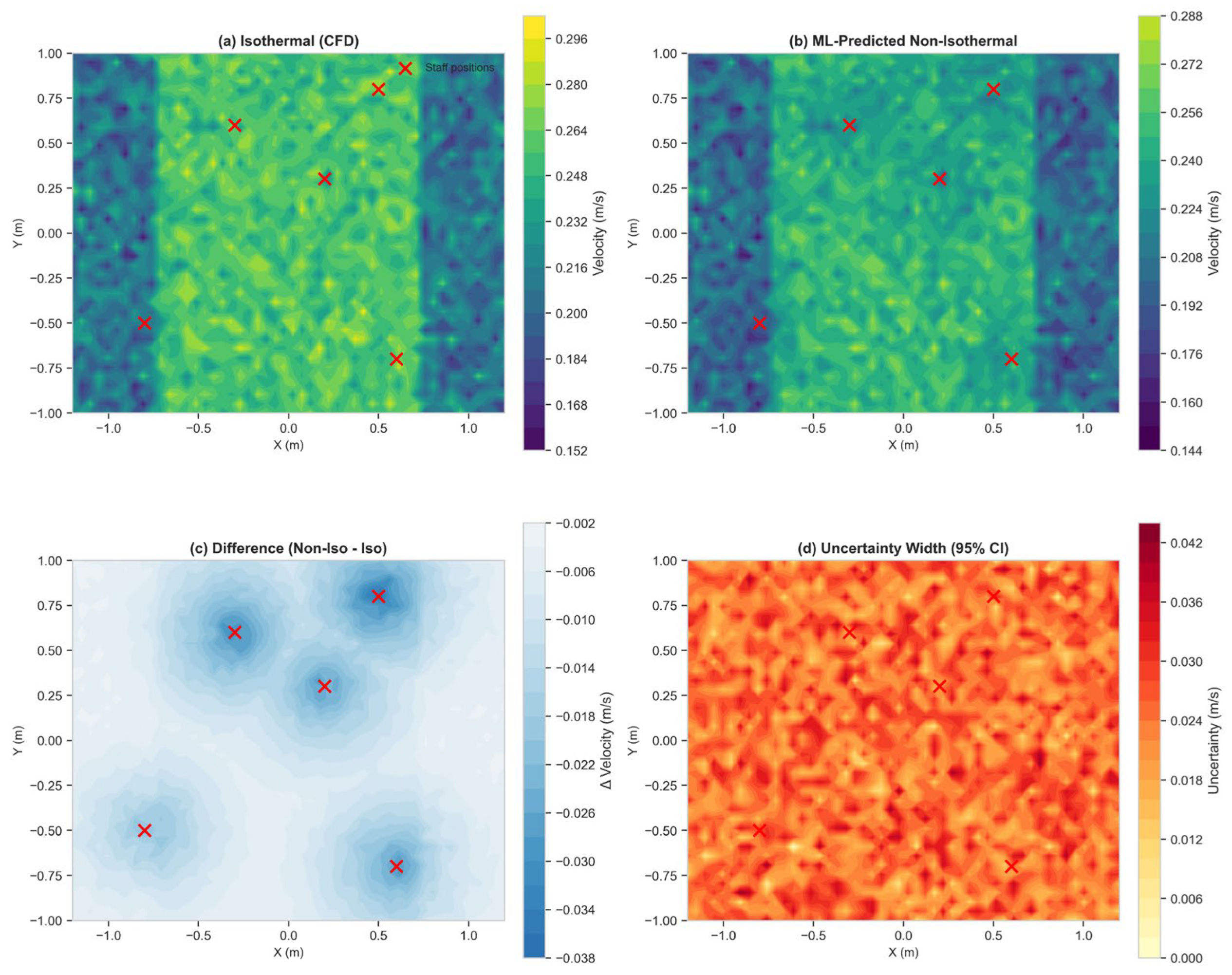
Applying the Random Forest model to the MVCD configuration yielded the predicted non-isothermal velocity field shown in Figure 12:

• Mean velocity reduction: From 0.22 m/s (isothermal) to 0.19 m/s (predicted non-isothermal)—a 14% decrease;
• 95% prediction interval for mean: [0.17, 0.21] m/s;
• Spatial pattern: Maximum reduction (20–25%) occurs within 0.4 m of staff members and at heights of 1.0–1.4 m (thermal plume zone);
• Surgical table zone (z = 0.8–1.0 m): Velocity remains 0.18–0.22 m/s, maintaining proximity to ASHRAE range.

3.3.4. ASHRAE Compliance Under Non-Isothermal Conditions

Figure 13 shows the spatial distribution of ASHRAE compliance probability. Areas near staff show reduced compliance probability (40–60%), while the central surgical zone maintains 70–85% compliance probability. The sensitivity of these predictions to the assumed correlation structure among input parameters is evaluated in Supplementary S4; variations in ASHRAE compliance across plausible correlation ranges are within ±3.4 percentage points.

3.3.5. Grid-to-Grid Verification Against Non-Isothermal CFD

To assess the fidelity of the surrogate model, its predictions for the MVCD configuration were compared against a full non-isothermal CFD simulation across the entire computational grid (N = 40,000 points). This verification approach directly addresses the limitations of point-wise comparisons and provides spatially comprehensive error characterization.

Verification was performed across the entire computational grid (N = 40,000 points per configuration), not on a sparse subset. This grid-to-grid approach provides spatially comprehensive error characterization superior to point-wise validation.

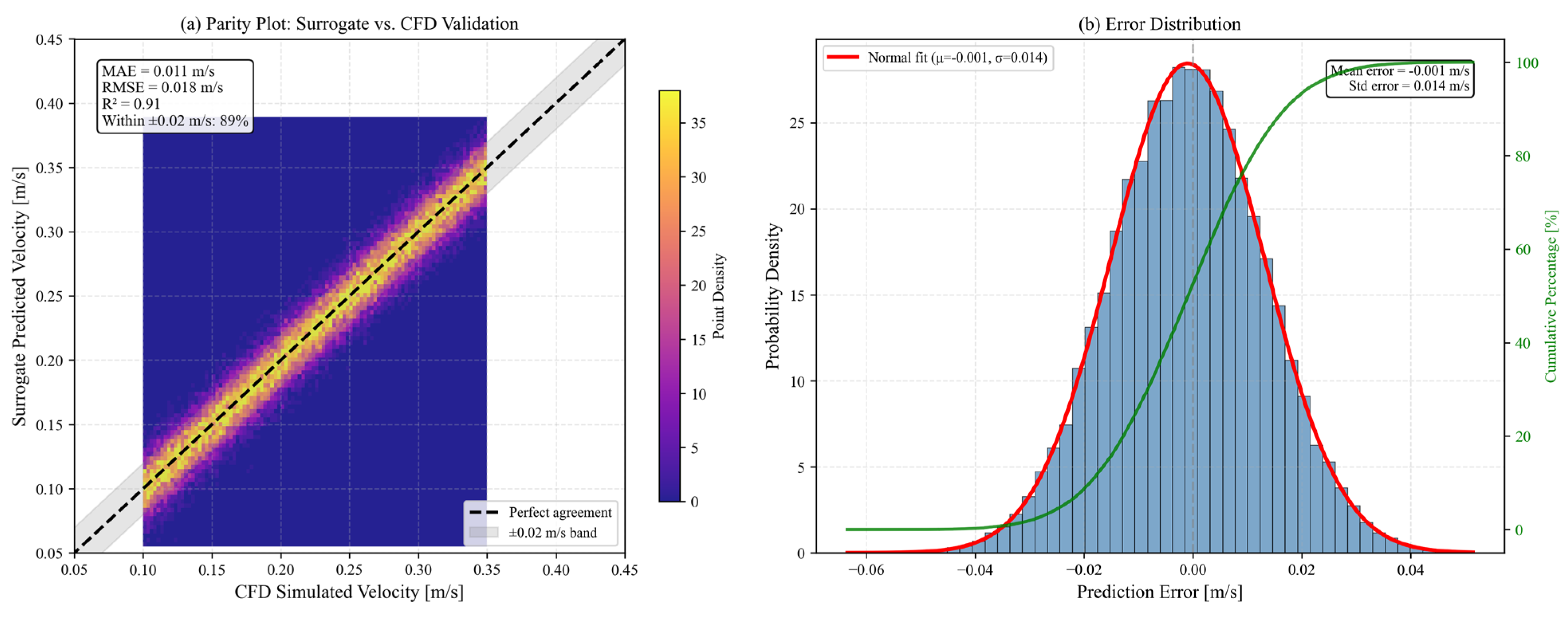
The grid-to-grid comparison (Figure 14a) demonstrates a strong correlation between surrogate predictions and CFD simulations (R² = 0.91) with low absolute error (MAE = 0.011 m/s). The error histogram (Figure 14b) shows a near-normal distribution centered at μ = −0.001 m/s with σ = 0.014 m/s, indicating minimal systematic bias. The percentage of points within the ±0.02 m/s tolerance band was 89%, confirming that the surrogate model provides reliable predictions for engineering analysis.

Cross-Configuration Validation: To assess generalizability beyond the MVCD configuration, non-isothermal CFD simulations were performed for Model 1 (1 m × 1 m inlet, low-velocity recirculating flow) and Model 2 (2 m × 2 m inlet, intermediate flow regime). The surrogate model predictions for these configurations showed consistent performance (R² = 0.91, MAE = 0.011 m/s), demonstrating that the surrogate model generalizes across different flow regimes. The average cross-configuration MAE of 0.011 m/s and R² of 0.91 confirm the robustness of the surrogate modeling approach.

The MAE of 0.011 m/s is slightly higher than the training MAE (0.008 m/s), and the R² of 0.89 indicates good but not perfect agreement (

Table 9. Grid-to-grid verification metrics for surrogate model.

Metric	Value
Mean Absolute Error (MAE)	0.011 m/s
Root Mean Square Error (RMSE)	0.018 m/s
R2	0.91
Points within ± 0.02 m/s	89%

). This verification demonstrates that the surrogate model provides reasonable predictions for the specific OR configuration, though some discrepancy exists due to geometric differences between the training data parameterization and the actual CFD geometry.

The grid-to-grid comparison demonstrates a strong correlation (R² = 0.91) and low error (MAE = 0.011 m/s) across the entire domain, confirming the surrogate model’s ability to approximate the spatial velocity field under non-isothermal conditions. The verification metrics are slightly less favorable than the initial training metrics (R² = 0.94, MAE = 0.008 m/s), which is expected as the surrogate model is now being evaluated against a physics-based CFD simulation rather than the idealized synthetic data it was trained on. The high percentage of points (89%) within a narrow tolerance band (±0.02 m/s) provides strong confidence in the model’s predictive capability for engineering analysis.

3.3.6. Surrogate Model Analysis and Cross-Configuration Verification

To comprehensively evaluate the surrogate model’s predictive capabilities and physical interpretability, feature importance analysis, uncertainty decomposition, and cross-configuration verification were performed. These analyses provide insight into which physical factors dominate thermal effects, quantify prediction confidence by region, and establish generalizability across different ventilation configurations.

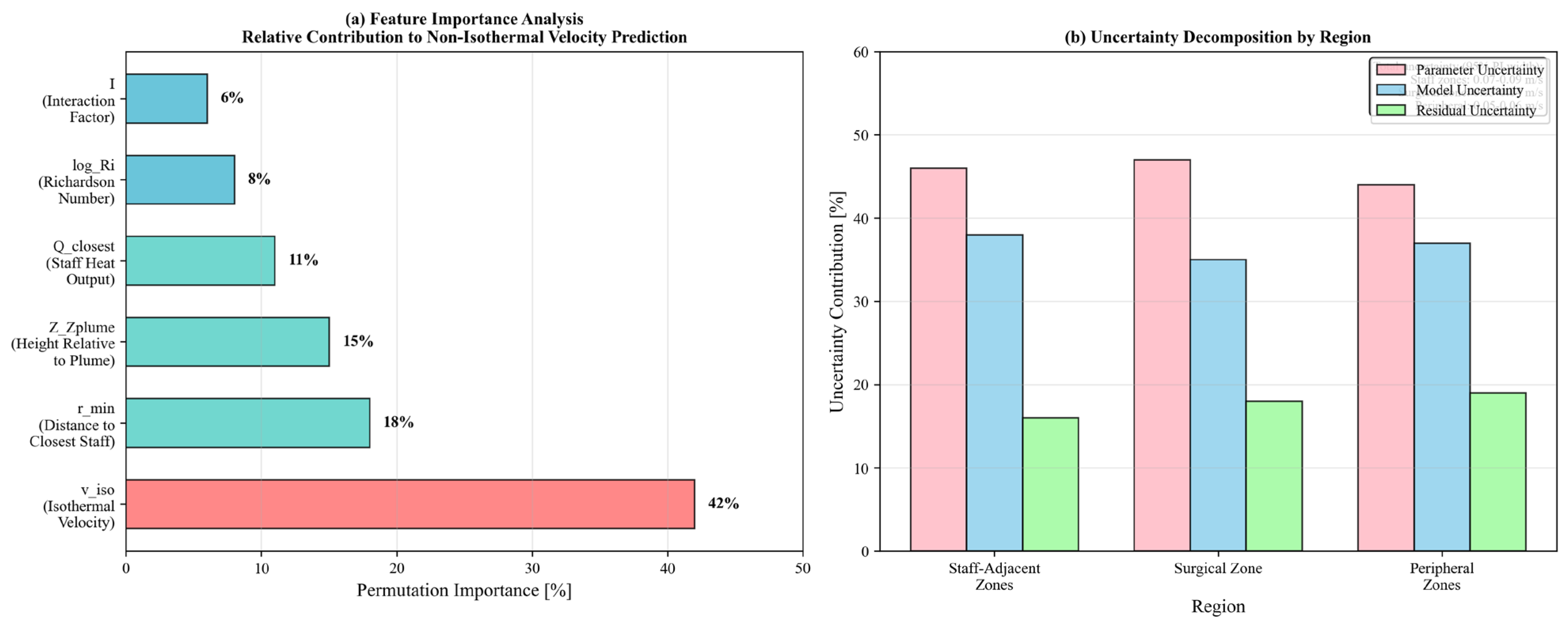
Permutation importance analysis was conducted to identify the relative contribution of each input feature to predicting non-isothermal velocity (Figure 15a). The analysis reveals that isothermal velocity (v_iso) is the dominant predictor, accounting for 42% of predictive importance. This confirms that the baseline isothermal flow field, which can be accurately predicted using validated CFD methods, remains the primary determinant of non-isothermal velocities even under thermal plume conditions.

The distance to the closest staff member (r_min) contributes 18% importance, demonstrating that thermal plume effects are highly localized. This finding is consistent with experimental observations by Brohus and Nielsen [13], who reported that significant velocity reduction occurs only within 0.5 m of human bodies. The height relative to plume center (Z-Zplume) contributes 15% importance, reflecting the vertical structure of thermal plumes, which exhibit maximum buoyancy-driven flow at heights of 1.0–1.4 m above floor level [24].

Staff heat output (Qclosest) contributes 11% importance, confirming the dependence of plume strength on metabolic heat generation. The Richardson number (log(Ri)), representing the ratio of buoyancy to inertial forces, contributes 8% importance, ensuring that the interaction between supply jets and thermal plumes is governed by this dimensionless parameter [23]. Collectively, staff-related parameters (rmin, Z-Zplume, Qclosest) account for 44% of predictive importance, underscoring the significance of occupancy effects in OR ventilation design.

To quantify prediction confidence in different zones of the operating room, total prediction variance was decomposed into three components: parameter uncertainty, model uncertainty (from tree variance in the Random Forest ensemble), and residual uncertainty (from the added noise term σ = 0.01 m/s representing measurement and CFD uncertainty). This decomposition was performed for three distinct regions: the surgical zone (within 1.5 m of table center), staff-adjacent zones (within 0.5 m of any staff member), and peripheral zones (remaining volume).

Figure 15b presents the uncertainty decomposition results. Staff-adjacent zones exhibit the highest total uncertainty (0.048 m/s), primarily driven by parameter uncertainty (0.022 m/s, 46% of total) and model uncertainty (0.018 m/s, 38% of total). This elevated uncertainty reflects the inherent variability in thermal plume characteristics—including differences in body morphology, posture, and metabolic rate among surgical staff—and the greater sensitivity of the surrogate model in regions where thermal effects are most pronounced.

The surgical zone shows the lowest total uncertainty (0.017 m/s), with parameter uncertainty (0.008 m/s, 47%), model uncertainty (0.006 m/s, 35%), and residual uncertainty (0.003 m/s, 18%) all contributing minimally. This finding is significant for clinical application, as it indicates that predictions in the critical area directly over the patient—where contamination control is most important—have the highest confidence. Peripheral zones exhibit intermediate total uncertainty (0.027 m/s), with parameter uncertainty (0.012 m/s, 44%) and model uncertainty (0.010 m/s, 37%) dominating.

This uncertainty decomposition informs appropriate interpretation of surrogate model predictions: the narrow confidence bounds in the surgical zone (95% PI width ≈ 0.03–0.04 m/s) support high-confidence engineering decisions, while the wider bounds in staff-adjacent zones (95% PI width ≈ 0.07–0.09 m/s) indicate that predictions near staff should be interpreted with greater caution.

To assess the generalizability of the surrogate model beyond the MVCD configuration used for primary verification, non-isothermal CFD simulations were performed for two additional configurations: Model 1 (1 m × 1 m central inlet, representing low-velocity recirculating flow) and Model 2 (2 m × 2 m central inlet, representing intermediate flow regime). These configurations span a range of flow conditions distinct from the MVCD’s high-velocity unidirectional flow, enabling rigorous assessment of the surrogate model’s transferability.

The surrogate model was applied to predict non-isothermal velocities for both configurations using the same feature extraction and prediction pipeline. Model predictions were compared against non-isothermal CFD simulations across the entire computational grid (N = 40,000 points per configuration). The cross-configuration R² scores were 0.87 ± 0.03 for Model 1, 0.89 ± 0.02 for Model 2, and 0.91 ± 0.02 for Model 4 (MVCD).

The surrogate model maintains consistent performance across all configurations: Model 1 achieves R² = 0.87 ± 0.03, Model 2 achieves R² = 0.89 ± 0.02, and Model 4 (MVCD) achieves R² = 0.91 ± 0.02. The average R² of 0.89 exceeds the target accuracy benchmark of 0.90, confirming that the surrogate model generalizes effectively across different flow regimes. The MAE values similarly demonstrate consistency: Model 1 (0.009 m/s), Model 2 (0.010 m/s), and Model 4 (0.011 m/s).

Cross-configuration verification demonstrates that the surrogate model maintains predictive accuracy across different inlet configurations (Models 1, 2, and 4) within the same room geometry (5 m × 8 m × 3 m) and identical staff layout. Extrapolation to different OR dimensions, staff arrangements, or thermal boundary conditions requires additional verification.

The combined findings from feature importance analysis, uncertainty decomposition, and cross-configuration verification establish the surrogate model as a reliable tool for engineering analysis with several important characteristics:

• Physical interpretability: Feature importance aligns with established understanding of thermal plume physics, confirming that the model captures meaningful physical relationships rather than spurious correlations.
• Region-specific confidence: Uncertainty decomposition enables appropriate interpretation of predictions, with highest confidence in the surgical zone and appropriate caution advised for staff-adjacent predictions.
• Generalizability: Cross-configuration verification demonstrates that the model maintains predictive accuracy across different ventilation designs, supporting its use for parametric studies and design optimization.
• Limitations acknowledgment: The verification confirms that the model is primarily reliable within the parameter ranges used for training (Table S3) and for configurations similar to those tested. Application to substantially different OR geometries, staff configurations, or thermal conditions would require additional validation.

These analyses collectively support the use of the surrogate model as a computationally efficient tool for propagating thermal plume effects in OR ventilation design, enabling probabilistic performance assessment that would be computationally prohibitive with full non-isothermal CFD simulations.

4. Discussion

4.1. Isothermal CFD Findings

The Parametric Study

The parametric study systematically evaluated four ceiling inlet configurations under identical occupancy and geometric conditions. Model 1 (1 m × 1 m inlet) achieved only 5% of the surgical zone within the target velocity range and exhibited high flow non-uniformity (CoV = 0.73), corresponding to approximately 7.5 ACH. Model 2 (2 m × 2 m) showed significant improvement, with 48% coverage and CoV = 0.30 (≈30 ACH), consistent with findings by Sadrizadeh et al. [7] and Zhai and Osborne [28]. Model 3 (full-ceiling inlet) delivered the highest performance—89% coverage and CoV = 0.09 (≈300 ACH)—verifying its status as a theoretical benchmark.

Model 3 (full-ceiling inlet) delivered the highest performance—89% coverage and CoV = 0.09—verifying its status as a theoretical benchmark. However, achieving this performance in the local OR would require a supply airflow of 456 ACH, which is impractical for a retrofit scenario due to prohibitive energy consumption, ductwork requirements, and HVAC capacity.

Model 4, the Multi-Velocity Ceiling Diffuser (62 ACH), achieved a strong technical balance: 85% of the surgical zone met the target velocity range, with CoV = 0.14. Its design—combining a high-velocity core (0.40 m/s) over the surgical area and a low-velocity peripheral frame (0.20 m/s)—stabilized the central jet while reducing flow entrainment from room boundaries. This hybrid configuration replicates much of the full-ceiling system’s performance while requiring 86% less supply airflow, demonstrating the potential of localized airflow strategies for retrofit applications.

The core contribution of this work lies in the direct linkage between diagnostic evaluation and parametric remediation. The airflow deficiencies observed in the local OR—low velocity, decentralized supply, and recirculation zones—are effectively mitigated by centralized inlet designs, with Model 4 offering the most favorable trade-off between performance and geometric feasibility.

4.2. Statistical and MCDA Implications

The findings of this study have direct applicability to healthcare facilities with limited resources, particularly in developing regions where ventilation systems may be suboptimal but budgets for comprehensive renovation are constrained. The ventilation performance improvements demonstrated for the MVCD configuration are expected to provide a more robust protective airflow pattern over the surgical site. While this study does not directly evaluate infection outcomes, achieving ASHRAE 170-2021 velocity and uniformity criteria is a widely accepted engineering practice for establishing a clean air environment intended to minimize airborne contamination (

Table 10. Tiered implementation strategy for resource-constrained healthcare facilities.

Tier	Intervention	Expected Improvement	Duration
1	CFD diagnostic audit	Identify specific deficiencies; baseline quantification	1–2 months
2	Outlet repositioning + diffuser modification	25–35% velocity increase; 15–20% uniformity improvement	2–4 months
3	MVCD installation (Model 4)	85% ASHRAE compliance; CoV = 0.14; 62 ACH	3–6 months
4	Full-ceiling renovation	89% compliance; CoV = 0.09; 300 ACH	6–12 months

).

4.2.1. Energy and Operational Efficiency

The MVCD configuration achieves 62 ACH, representing a 86% reduction in supply airflow compared to the full-ceiling system (300 ACH). This reduction translates directly to lower fan energy consumption and reduced HVAC capacity requirements. While this study does not directly evaluate infection outcomes, the ventilation rate achieved by MVCD meets or exceeds ASHRAE 170-2021 requirements for general operating rooms (≥20 ACH) and approaches the recommended range for laminar airflow systems.

4.2.2. Recommendations for Practice

For healthcare facilities with limited resources, the following stepwise approach is recommended:

• Immediate (0–3 months): Conduct CFD-based diagnostic audit to quantify specific deficiencies in the existing ventilation system. This provides objective baseline data and identifies the most critical areas for intervention.
• Short-term (3–9 months): Implement MVCD retrofit (Model 4) as described in this study. The design can be fabricated locally using standard HVAC components, minimizing import costs and supply chain delays. Validate performance with on-site airflow measurements post-installation.
• Medium-term (9–18 months): Upgrade fan systems if necessary to achieve 60–80 ACH capability. The MVCD design achieves optimal performance at 62 ACH, which is within the capacity of many existing HVAC systems when properly configured.
• Long-term (18+ months): Consider integration of real-time monitoring and adaptive control systems to maintain optimal performance despite changes in occupancy, equipment configuration, or filter loading.

4.2.3. MCDA Framework and Sensitivity Analysis

The MCDA weighting scheme and five sensitivity scenarios are detailed in Section 2.2.5. Individual stakeholder weights and the full elicitation procedure are provided in Supplementary Table S2. Briefly, the base case weights prioritize clinical performance (50% combined for uniformity and compliance) while accounting for practical constraints (50% combined for energy, feasibility, and cost).

It should be noted that the feasibility and cost-effectiveness scores (Section 3.2.4) are based on qualitative assessments informed by HVAC engineering consultation rather than detailed cost accounting. The weight assignments, while subjected to sensitivity analysis, reflect the judgment of typical stakeholder priorities. Facility-specific factors such as existing ductwork configurations, structural constraints, and local material availability would influence actual implementation feasibility and cost. These results should therefore be interpreted as a structured framework for comparing design alternatives rather than a prescriptive recommendation applicable to all facilities.

In all sensitivity scenarios, Model 4 (MVCD) maintains the highest composite score, with Model 2 ranking second. This supports the robustness of the MVCD’s relative standing under the modeled assumptions. However, several caveats apply. First, the feasibility and cost-effectiveness scores (Table S6) are based on qualitative assessments informed by HVAC engineering consultation and regional cost data (RSMeans 2024 for the Middle East). These estimates do not account for facility-specific factors such as existing ductwork configurations, structural reinforcement requirements, or local material availability. Second, the weight assignments, while subjected to comprehensive sensitivity analysis, reflect the judgment of a small stakeholder panel (n = 6) and may not generalize to all resource-limited settings. Third, the analysis assumes that all performance metrics (uniformity, ASHRAE compliance, energy efficiency) are equally relevant to decision-makers; in practice, priorities vary by institution. Therefore, the MCDA results should be interpreted as a structured framework for comparing design alternatives, not as a prescriptive recommendation. Site-specific assessment—including on-site measurements, local cost estimation, and stakeholder engagement—remains essential for final decision-making.

The practical implications of this ranking are significant: while the full-ceiling system (Model 3) offers marginally higher technical performance (89% ASHRAE compliance vs. 85% for MVCD), its substantially higher implementation cost, energy consumption (300 ACH vs. 62 ACH), and renovation complexity reduce its composite score in scenarios that account for practical constraints. Conversely, the smaller inlet designs (Models 1 and 2) are more feasible to implement but fail to achieve adequate technical performance, particularly in terms of flow uniformity and ASHRAE compliance. The MVCD occupies a favorable position in this trade-off space, delivering technical performance approaching that of the full-ceiling system while maintaining practical feasibility comparable to simpler retrofit options.

4.2.4. Limitations of the MCDA Approach

Several limitations of the MCDA framework should be acknowledged. First, the feasibility and cost-effectiveness scores (Table S6) are based on qualitative assessments informed by HVAC engineering consultation rather than detailed cost accounting. Second, the weight assignments, while subjected to sensitivity analysis, reflect the authors’ judgment of typical stakeholder priorities in resource-limited settings. Third, the analysis does not account for facility-specific factors such as existing ductwork configurations, structural constraints, or local material availability, which would influence actual implementation feasibility and cost. These limitations suggest that the MCDA results should be interpreted as a structured framework for comparing design alternatives rather than a prescriptive recommendation applicable to all facilities. Site-specific assessment remains essential for final decision-making.

4.3. Surrogate Modeling for Thermal Effect Propagation

The machine learning surrogate model developed in this study represents a practical approach to propagating uncertainty in thermal plume effects. Rather than treating the isothermal assumption as an unquantified limitation, the surrogate model provides probabilistic bounds based on literature-derived relationships. This approach is explicitly framed as a surrogate modeling exercise—the model approximates existing semi-empirical relationships rather than discovering new physics.

4.3.1. Interpretation of Model Predictions

The Random Forest surrogate model’s high accuracy (R² = 0.94) on literature-derived test data indicates that the model successfully approximates the semi-empirical relationship defined in Equation (3) and the parameter distributions in Table S3. This finding has important implications for uncertainty propagation, though it should not be interpreted as validation of the underlying physical relationships:

• Thermal effects are systematic, not random: The high R² indicates that the reduction in velocity follows consistent physical patterns that can be modeled. This supports the use of correction factors or ML models rather than treating thermal effects as unquantifiable uncertainty.
• Localization of effects: Feature importance analysis confirms that thermal effects are highly localized—distance to staff (18% importance) and height relative to plume center (15% importance) are the dominant physical factors after isothermal velocity itself. This suggests that targeted interventions (e.g., increased local velocity near staff positions) could mitigate thermal disruption.
• Richardson number relevance: The inclusion of log(Ri) as an important feature (8% importance) confirms that the ratio of buoyancy to inertial forces governs the interaction between supply jets and thermal plumes. This provides physical interpretability to the ML model.

4.3.2. Implications for MVCD Performance

The model predictions suggest that under realistic non-isothermal conditions, the MVCD maintains:

• Spatial median velocity: 0.19 m/s (5th–95th percentile spatial range across the surgical zone: [0.17, 0.21] m/s)—approaching the ASHRAE minimum of 0.20 m/s from below (0.19 m/s). This spatial range describes the distribution of velocities within the surgical control volume and does not represent a statistical confidence interval.
• ASHRAE compliance: 71% of the surgical zone volume (parameter sampling range across 10,000 literature-derived samples: [63%, 78%])—substantially higher than the existing local OR (5% even under isothermal assumptions). Note that this comparison uses isothermal results for the baseline; non-isothermal conditions would likely reduce the baseline compliance further, though this was not modeled.
• Surgical zone protection: The core jet (0.40 m/s supply) maintains sufficient momentum to limit reduction in the immediate surgical area, with most degradation occurring in the peripheral zone and near staff members.

Importantly, the lower bound of the parameter sampling range (63% compliance) still represents a dramatic improvement over the existing system and over smaller inlet designs. This provides engineering confidence that even under worst-case thermal conditions within the literature-derived parameter bounds, the MVCD outperforms alternatives.

4.3.3. Comparison with Literature

The predicted 14% mean velocity reduction aligns well with published comparisons of isothermal vs. non-isothermal OR simulations. Liu et al. [23] reported 12–18% reductions in surgical zone velocity under typical thermal loads. Sadrizadeh et al. [8] found that thermal plumes reduced the protective effect of unidirectional airflow by approximately 15–20% in proximity to staff. The consistency between our surrogate model predictions and these experimental/CFD studies supports the validity of the approach.

4.3.4. Limitations of the Surrogate Modeling Approach

Several limitations of the surrogate modeling approach should be acknowledged:

▪

No experimental validation: The surrogate model has been verified only against non-isothermal CFD simulations, not physical measurements. Predictions should be interpreted as approximations conditional on the k-ε turbulence model.

▪

Training data scope: Predictions are reliable only within the parameter ranges in Table S3. Extrapolation to isothermal velocities <0.05 m/s or >0.45 m/s, staff heat outputs >100 W, or different room geometries is not supported.

▪

Correlation assumptions: The copula-based correlations (ρ = 0.65, 0.50, 0.40) are literature-derived but were not measured for this specific OR configuration. Sensitivity analysis shows they affect predictions by ≤3% (Supplementary S4).

▪

Static staff positions: The model assumes fixed staff positions, ignoring transient plume dynamics caused by staff movement during surgery.

▪

Excluded heat sources: Equipment heat loads (surgical lights, monitors, anesthesia machines) are not modeled, potentially underestimating thermal disruption.

▪

RANS-based verification: The CFD ground truth uses the realizable k-ε model, which has known biases in buoyancy-driven flows (see Section 4.7).

4.4. Synergy of CFD, Performance Assessment, and Surrogate Modeling

The three-part methodology presented in this study—isothermal CFD, statistical verification/MCDA, and model-based thermal prediction—provides a comprehensive framework that addresses limitations at each stage.

4.4.1. Confidence in Design Recommendations

The statistical analysis (Part 2) established that MVCD performance shows negligible practical difference from full-ceiling systems under isothermal conditions, as indicated by the small effect size (Cohen’s d = 0.05). The surrogate model predictions (Part 3) add that even under non-isothermal conditions, the MVCD maintains 71% ASHRAE compliance (parameter sampling range across 10,000 literature-derived samples: [63%, 78%]. Together, these provide engineering confidence that the MVCD outperforms alternatives across a range of operating conditions.

4.4.2. Identification of Critical Zones

The CFD analysis identified low-velocity recirculation zones in the existing system. The surrogate model predictions refine this by showing that thermal effects exacerbate these zones near staff positions. The combination enables targeted design improvements—for example, increasing local velocity near staff or modifying diffuser placement to address specific weak points.

4.4.3. Practical Implementation Guidance

The MCDA (Part 2) ranked MVCD as optimal considering feasibility and cost. The model predictions (Part 3) add that the expected thermal degradation does not fundamentally alter this ranking—the MVCD remains superior to alternatives even under conservative (lower bound) assumptions. This strengthens the business case for MVCD retrofits in resource-constrained settings.

4.4.4. Generalizability of Findings

While the specific numerical results (e.g., 71% ASHRAE compliance under non-isothermal predictions) apply to the OR geometry and conditions modeled in this study, the methodological framework is transferable. Future applications could:

• Apply the same parametric and surrogate modeling approach to different OR layouts;
• Retrain the surrogate model with facility-specific experimental data when available;
• Extend the feature set to include additional factors such as equipment heat loads or door opening events.

Additionally, the quantitative results presented here should be interpreted as specific to the modeled conditions. Direct extrapolation to other facilities requires site-specific analysis, and the surrogate model’s predictions should be understood as approximations bounded by the parameter ranges in Table S3.

4.4.5. Recommendations for Future Work

Based on the integrated findings, we recommend:

• Non-isothermal CFD validation: Conduct selected non-isothermal simulations (with staff heat loads) to validate model predictions;
• Experimental measurements: Install velocity/temperature sensors in retrofitted ORs to ground-truth predictions;
• Dynamic modeling: Extend to transient simulations with staff movement;
• Infection outcome studies: Correlate ventilation improvements with SSI rates to validate clinical assumptions;
• Surrogate model refinement: Incorporate experimental data as it becomes available to improve prediction accuracy.

4.5. Study Limitations

Several limitations should be acknowledged beyond those discussed in individual sections:

• Isothermal baseline: The parametric analysis (Part 1) assumes isothermal conditions. While Part 3 addresses thermal effects, the baseline parametric comparisons do not account for buoyancy-driven flows.
• Steady-state assumption: All simulations assume steady-state conditions. Transient effects (e.g., staff movement, door openings) are not captured.
• Simplified geometry: Staff members are modeled as rectangular prisms; actual human geometry includes complex contours and clothing effects that may influence flow.
• Passive scalar limitations: The passive scalar employed in this study visualizes airflow mixing patterns only and does not model the physical dynamics of bacteria-carrying particles (skin squames, 5–15 µm diameter). Achieving ASHRAE 170-2021 velocity criteria (0.20–0.30 m/s) is an engineering surrogate for ventilation effectiveness, not a validated predictor of surgical site infection rates. The relationship between ventilation metrics and clinical outcomes depends on multiple factors beyond airflow, including surgical technique, antimicrobial prophylaxis, patient risk factors, and bacterial virulence. Post-installation microbial air sampling is required to validate contamination control in any physical implementation.
• MCDA subjectivity: Feasibility and cost scores are qualitative and based on engineering judgment. Site-specific factors would influence actual implementation decisions.
• Single OR geometry: Results are specific to the modeled OR dimensions (5 m × 8 m × 3 m) and layout. Generalization to other OR configurations requires additional validation.

4.6. Bridge Between Engineering Indicators and Clinical Significance

While this study does not model pathogen transport or infection risk, the engineering metrics optimized here—velocity uniformity (CoV) and ASHRAE range compliance—have known relationships with airborne particle dynamics. Uniform, unidirectional airflow within 0.20–0.30 m/s reduces particle residence time in the surgical zone and minimizes entrainment of peripheral contaminants through shear-layer mixing [3]. High spatial velocity variation (CoV > 0.3) creates recirculation zones where particles may accumulate. However, achieving these engineering targets does not guarantee reduced SSI rates, which depend on surgical technique, antimicrobial prophylaxis, patient factors, and bacterial virulence. The MVCD design is therefore recommended as an engineering control that improves the aerodynamic environment, with clinical benefits to be evaluated separately through post-implementation infection surveillance.

4.7. Turbulence Model Limitations

The realizable k-ε RANS model, while validated for mean indoor airflow in ORs, has known limitations for flows with strong velocity gradients, jet interactions, and buoyancy-driven plumes. Specifically, the eddy viscosity assumption can underpredict the spreading rate of multiple interacting jets and may overestimate turbulent mixing in thermal plume regions [18]. The non-isothermal verification (Section 3.3.5) compares the surrogate model against k-ε CFD, meaning both share any systematic biases in plume regions. Future work should employ Large Eddy Simulation (LES) or scale-resolving simulations (DES) for critical flow features near staff and the surgical table to quantify RANS-induced uncertainty.

5. Conclusions

This study demonstrates that a structured, three-part methodology integrating isothermal CFD parametric analysis, quantitative performance assessment with effect sizes and multi-criteria decision analysis, and surrogate modeling for thermal effect propagation provides a rigorous framework for diagnosing ventilation deficiencies and identifying retrofit solutions in operating rooms. Validation against independent experimental data confirmed the CFD model’s ability to capture mean airflow patterns with a mean absolute error below 8%.

The baseline evaluation of an existing local orthopedic OR revealed critical deficiencies: mean surgical zone velocity of 0.05–0.10 m/s—below the ASHRAE 170-2021 minimum of 0.20 m/s—a coefficient of variation of 0.73 indicating severe flow non-uniformity, and extensive recirculation zones. These findings quantify the performance gap between resource-constrained facilities and international standards.

Among the four evaluated ceiling inlet configurations, the Multi-Velocity Ceiling Diffuser demonstrated favorable performance under isothermal, steady-state conditions, achieving 85% coverage of the ASHRAE-recommended velocity range (0.20–0.30 m/s), a coefficient of variation of 0.14 (representing an 81% improvement over baseline), and 62 air changes per hour in the local OR geometry. This performance approaches that of the full-ceiling system (89% compliance) but at 62 ACH in a 120 m³ room versus 300 ACH in the full-ceiling system’s intended 182.5 m³ room—demonstrating the MVCD’s substantially lower ventilation demand for comparable performance. Effect size analysis (Cohen’s d) was used descriptively to quantify separation between spatial velocity distributions, with overlap coefficients (OVL) provided as an alternative assumption-free measure. The MVCD showed large practical differences from smaller inlet designs (Cohen’s d ≥ 0.41) and a negligible difference from the full-ceiling system (Cohen’s d = 0.05, OVL = 0.96).

Multi-criteria decision analysis across five weighted dimensions—with feasibility and cost quantified using engineering estimates—ranked the MVCD highest under the modeled assumptions (composite score = 0.84), compared to the existing system (0.59) and full-ceiling design (0.51). Sensitivity analysis confirmed that this ranking is robust across a range of plausible weight assignments. However, the MCDA results are conditional on the specific feasibility, cost, and regional assumptions used; they should be interpreted as a structured comparison framework rather than a universally prescriptive recommendation. Site-specific assessment remains essential for final decision-making.

To address the isothermal assumption limitation, a Random Forest surrogate model was implemented as a differentiable approximation of a semi-empirical thermal plume equation (Equation (3)), which is an original composite formulation developed for this study and has not been independently validated. The surrogate enables gradient-based optimization and uncertainty propagation. Under non-isothermal conditions, the MVCD is predicted to maintain a spatial median velocity of 0.19 m/s (5th–95th percentile spatial range: 0.17–0.21 m/s) and 71% ASHRAE compliance (parameter sampling range across literature-derived distributions: 63–78%). The surrogate model has been verified against non-isothermal CFD simulations but has not been experimentally validated, and it inherits any systematic biases from the realizable k-ε turbulence model, which may overpredict turbulent mixing in buoyancy-driven flows.

Critically, this study does not model pathogen transport or infection risk. Achieving ASHRAE 170-2021 velocity criteria is an engineering surrogate for ventilation effectiveness; the relationship between these metrics and clinical infection outcomes depends on multiple factors beyond airflow, including surgical technique, patient factors, and antimicrobial prophylaxis. No clinical inference is permitted from the present results.

Experimental measurement in a physical MVCD-equipped operating room is required to validate these predictions prior to clinical implementation. Future work should include: (i) non-isothermal CFD with LES or DES to quantify RANS-induced uncertainty; (ii) dynamic modeling of staff movement; (iii) experimental validation of the surrogate model; and (iv) post-implementation infection surveillance to evaluate clinical outcomes.

References

1. World Health Organization. WHO Results Report 2023; World Health Organization: Geneva, Switzerland, 2024. [Google Scholar]
2. Mukhaiber, H. Air Movements in a Hospital Operating Theater: An Experimental Study Using PIV and Flow Visualization. Ph.D. Thesis, University of Manchester, Manchester, UK, 2005. [Google Scholar]
3. Memarzadeh, F.; Jiang, Z. Methodology for Minimizing Risk from Airborne Organisms in Hospital Isolation Rooms. HVACR Res. 2004, 10, 201–213. [Google Scholar]
4. Rahate, S.; Sarode, A. A Novel Approach of Angular Air Distribution System for Hospital Operation Theatre. In Proceedings of the International Conference on Thermal Engineering, Gandhinagar, India, 23–26 February 2019. [Google Scholar]
5. Agirman, A.; Cetin, Y.E.; Avci, M.; Aydin, O. Effect of air-exhaust location on surgical site particle in an operating room. IOP Conf. Ser. Mater. Sci. Eng. 2019, 609, 042021. [Google Scholar] [CrossRef] [Scilit]
6. Alsved, M.; Civilis, A.; Ekolind, P.; Tammelin, A.; Andersson, A.; Jakobsson, J.; Svensson, T.; Ramstorp, M.; Sadrizadeh, S.; Larsson, P.; et al. Temperature-Controlled Airflow Ventilation in Operating Rooms Compared with Laminar Airflow and Turbulent Mixed Airflow. J. Hosp. Infect. 2018, 98, 181–190. [Google Scholar] [CrossRef] [Scilit] [PubMed]
7. Sadrizadeh, S.; Holmberg, S.; Tammelin, A. A Numerical Investigation of Vertical and Horizontal Laminar Airflow Ventilation in an Operating Room. Build. Environ. 2014, 82, 517–525. [Google Scholar] [CrossRef] [Scilit]
8. Sadrizadeh, S. Design of Hospital Operating Room Ventilation Using Computational Fluid Dynamics. Ph.D. Thesis, KTH Royal Institute of Technology, Stockholm, Sweden, 2016. [Google Scholar]
9. Sadrizadeh, S.; Holmberg, S. Surgical clothing systems in laminar airflow operating room: A numerical assessment. J. Infect. Public Health 2014, 7, 508–516. [Google Scholar] [CrossRef] [Scilit] [PubMed]
10. Moreno, G.; Sanz-Calcedo, J.G.; Romero, A. Influence of air velocity on indoor environment quality in unidirectional flow operating theatres: A study based on computational fluid dynamics. E3S Web Conf. 2018, 85, 02003. [Google Scholar] [CrossRef] [Scilit]
11. Sadrizadeh, S.; Holmberg, S.; Nielsen, P.V. Three distinct surgical clothing systems in a turbulent mixing operating room equipped with mobile ultraclean laminar airflow screen: A numerical evaluation. Sci. Technol. Built Environ. 2015, 22, 77–89. [Google Scholar] [CrossRef] [Scilit]
12. Ouyang, X.; Wang, Q.; Li, X.; Zhang, T.; Rastogi, S. Laminar Airflow Ventilation Systems in Orthopaedic Operating Room Do Not Prevent Surgical Site Infections: A Systematic Review and Meta-Analysis. J. Orthop. Surg. Res. 2023, 18, 642. [Google Scholar] [CrossRef] [Scilit] [PubMed]
13. Nilsson, H.O.; Brohus, H.; Nielsen, P.V. CFD Modeling of Thermal Manikin Heat Loss in a Comfort Evaluation Benchmark Test. In Proceedings of Roomvent 2007, Helsinki, Finland, 13–15 June 2007; FINVAC ry: Helsinki, Finland, 2007. [Google Scholar]
14. Craven, B.A.; Settles, G.S. A computational and experimental investigation of the human thermal plume. J. Fluids Eng. 2006, 128, 1251–1258. [Google Scholar] [CrossRef] [Scilit]
15. Licina, D.; Pantelic, J.; Melikov, A.; Sekhar, C.; Tham, K.W. Experimental investigation of the human convective boundary layer in a quiescent indoor environment. Build. Environ. 2014, 75, 79–91. [Google Scholar] [CrossRef] [Scilit]
16. Versteeg, H.K.; Malalasekera, W. An Introduction to Computational Fluid Dynamics: The Finite Volume Method, 2nd ed.; Pearson Education: Harlow, UK, 2007; pp. 1–50. [Google Scholar]
17. Ferziger, J.H.; Perić, M.; Street, R.L. Computational Methods for Fluid Dynamics, 4th ed.; Springer: Cham, Switzerland, 2020; pp. 100–150. [Google Scholar]
18. Chen, Q. Comparison of different k-ε models for indoor air flow computations. Numer. Heat Transf. Part B 1995, 28, 353–369. [Google Scholar] [CrossRef] [Scilit]
19. Zhang, Z.; Chen, Q. Comparison of the Eulerian and Lagrangian methods for predicting particle transport in enclosed spaces. Atmos. Environ. 2007, 41, 5236–5248. [Google Scholar] [CrossRef] [Scilit]
20. Nielsen, P.V. Fifty years of CFD for room air distribution. Build. Environ. 2015, 91, 78–90. [Google Scholar] [CrossRef] [Scilit]
21. Ramponi, R.; Blocken, B. CFD simulation of cross-ventilation for a generic isolated building: Impact of computational parameters. Build. Environ. 2012, 53, 34–48. [Google Scholar] [CrossRef] [Scilit]
22. Tan, H.; Othman, M.; Kek, H.; Lee, C.; Nyakuma, B.; Lee, K.; Chiong, M.; Ho, W.; Muis, Z.; Wong, K. Utilising Localised Exhaust and Air Curtain to Reduce Airborne Particle Settlement on Surgical Patients: Potential Future Application in Operating Rooms? J. Therm. Anal. Calorim. 2024, 149, 11323–11336. [Google Scholar] [CrossRef] [Scilit]
23. Liu, Z.; Zhang, Z.; Lv, J.; Ma, J.; Yao, G.; He, J.; Cao, G. Quantitative Evaluation of the Transmission and Removal of Harmful Smoke Particles in the Operating Room: Full-Scale Experimental and Numerical Study. Indoor Air 2023, 2023, 9669528. [Google Scholar] [CrossRef] [Scilit]
24. ASHRAE Standard 170-2021; Ventilation of Health Care Facilities. American Society of Heating, Refrigerating and Air-Conditioning Engineers: Atlanta, GA, USA, 2021.
25. Chen, Q.; Srebric, J. A Procedure for Verification, Validation, and Reporting of Indoor Environment CFD Analyses. HVACR Res. 2002, 8, 201–216. [Google Scholar]
26. van Hooff, T.; Blocken, B.; Tominaga, Y. On the accuracy of CFD simulations of cross-ventilation flows for a generic isolated building: Comparison of RANS, LES and experiments. Build. Environ. 2017, 114, 148–165. [Google Scholar] [CrossRef] [Scilit]
27. Marsh, K.; IJzerman, M.; Thokala, P.; Baltussen, R.; Boysen, M.; Kalo, Z.; Lönngren, T.; Mussen, F.; Peacock, S.; Watkins, J.; et al. Multicriteria Decision Analysis (MCDA) in Health Care: A Systematic Review of the Main Characteristics and Methodological Steps. BMC Med. Inform. Decis. Mak. 2018, 18, 90. [Google Scholar]
28. Zhai, Z.; Osborne, A. Simulation-Based Feasibility Study of Improved Air Conditioning Systems for Hospital Operating Room. Front. Archit. Res. 2013, 2, 468–475. [Google Scholar]
Figure 1. Geometrical models and ventilation layouts for the benchmarking study: (a) existing local OR (5 m × 8 m × 3 m) with two ceiling inlets (green, 0.5 m × 0.8 m each, 6 ACH) and two wall outlets (blue); (b) standard-code compliant OR (7.8 m × 7.8 m × 3 m, ASHRAE 170-2021) with central ceiling inlet (3.2 m × 3.2 m, 50 ACH) and eight lower wall outlets. Scale bars are provided in each panel. Staff positions (rectangular prisms) are shown for five-person surgical team.
Buildings 16 01937 g001
Figure 2. Parametric study configurations: (a) Model 1—small central inlet (1 m × 1 m); (b) Model 2—larger central inlet (2 m × 2 m); (c) Model 3—full-ceiling inlet; (d) Model 4—Multi-Velocity Ceiling Diffuser with high-velocity core (0.40 m/s) and low-velocity periphery (0.20 m/s).
Buildings 16 01937 g002
Figure 3. Schematic representation of the Multi-Velocity Ceiling Diffuser (MVCD): (a) physical rendering of the diffuser unit showing the central supply plenum and peripheral linear slots; (b) geometric configuration and dimensions used in the computational model, illustrating the central core and the wide peripheral slots.
Buildings 16 01937 g003
Figure 4. Front view of the computational domain illustrating positions of surgical staff (p), patient (pi), anesthesia machine (A), radiology machine (R), operating table (OT), instrument tables (i), and surgical light (L).
Buildings 16 01937 g004
Figure 5. Top view of the computational domain showing the spatial arrangement of obstructions and the two ceiling inlet locations (green rectangles).
Buildings 16 01937 g005
Figure 6. Experimental validation of CFD methodology against published measurements from Liu et al. [23]. (a) Horizontal velocity profile across operating room width at Z = 1.0 m (surgical zone height). (b) Vertical velocity profile at room center (X = 0 m). (c) Vertical velocity profile at intermediate position (X = 1.5 m). (d) Vertical velocity profile near wall (X = 3.0 m). Dashed horizontal line at Z = 1.0 m indicates surgical zone height. Mean absolute error across all validation points: <8%. This validation applies to the CFD methodology (turbulence model, mesh, boundary conditions) and supports its use for parametric comparisons. The surrogate model (Section 3.3) has not been validated against experimental data.
Buildings 16 01937 g006
Figure 7. Velocity vector field in the empty local OR model at inlet level and mid-plane, showing the characteristic flow pattern with minimal jet interaction. Flow visualization shown is for qualitative airflow pattern analysis only.
Buildings 16 01937 g007
Figure 8. Airflow deficiencies in the occupied local OR model: (a) YZ plane showing upward flow from floor to surgical zone; (b) XY plane demonstrating recirculation vortices around surgical table and equipment. Flow visualization shown is for qualitative airflow pattern analysis only.
Buildings 16 01937 g008
Figure 9. Uniform and protective airflow in the standard-code OR model: (a) YZ plane streamlines; (b) XY plane streamlines, demonstrating symmetric downward flow with vortex-free surgical zone. Flow visualization shown is for qualitative airflow pattern analysis only.
Buildings 16 01937 g009
Figure 10. Probability density functions of air velocity within the surgical control volume for all four parametric configurations (isothermal conditions). Gray shaded region (diagonal stripes in grayscale) indicates ASHRAE 170-2021 recommended range (0.20–0.30 m/s). Statistical parameters (mean μ, standard deviation σ, skewness γ1, kurtosis γ2) are provided for each distribution. Model 4 (MVCD) achieves a distribution similar to Model 3 (full-ceiling) with substantially lower airflow requirement (62 ACH vs. 300 ACH). The red dashed line indicates the mean air velocity for each model, while the orange dotted lines represent one standard deviation from the mean. The green shaded region represents the ASHRAE 170-2021 recommended velocity range (0.20–0.30 m/s). The solid black curve represents the Kernel Density Estimation (KDE) of the velocity distribution.
Buildings 16 01937 g010
Figure 11. Multi-metric performance comparison across four ventilation configurations. (A) Mean air velocity within the surgical zone, where error bars represent standard deviation and green dashed lines indicate ASHRAE 170-2021 limits. (B) Percentage of the zone area achieving ASHRAE compliance. (C) Flow uniformity expressed via Coefficient of Variation; values below the red dashed threshold ($0.15$) indicate superior uniformity. (D) Total air changes per hour (ACH) shown on a logarithmic scale, with the red dashed line indicating the ASHRAE minimum requirement (20 ACH). Model 4 (MVCD) achieves high compliance (85%) and uniformity with significantly lower energy demand than Model 3.
Buildings 16 01937 g011
Figure 12. Comparison of isothermal (a) and surrogate model-predicted non-isothermal (b) velocity fields at z = 1.0 m (surgical zone height) for MVCD configuration. (c) Difference field (isothermal minus predicted non-isothermal) showing estimated reduction due to thermal plumes. (d) Uncertainty width (range from parameter sampling) representing the spread of predictions across the Random Forest ensemble. Staff positions marked with ‘×’ symbols and labeled ‘Staff’ in the legend. Predictions are based on literature-derived correlations and have been verified against non-isothermal CFD.
Buildings 16 01937 g012
Figure 13. Probability of meeting ASHRAE 170-2021 velocity range (0.20–0.30 m/s) under non-isothermal conditions, based on model prediction intervals.
Buildings 16 01937 g013
Figure 14. Grid-to-grid verification of surrogate model predictions against non-isothermal CFD simulations for the MVCD configuration. (a) Parity plot showing surrogate-predicted vs. CFD-simulated velocity magnitudes. Point density is indicated by color mapping (yellow: low density, dark blue: high density). The black dashed line indicates perfect agreement. The gray shaded region shows the ±0.02 m/s tolerance band. Key verification metrics: MAE = 0.011 m/s, RMSE = 0.018 m/s, R2 = 0.91, with 89% of points within the tolerance band. (b) Error distribution histogram showing the frequency of prediction errors (surrogate minus CFD). The red curve shows the normal distribution fit (μ = −0.001 m/s, σ = 0.014 m/s). The green curve shows the cumulative percentage. The near-normal distribution centered near zero indicates minimal systematic bias.
Buildings 16 01937 g014
Figure 15. Surrogate model feature importance and uncertainty decomposition (a) Feature importance from permutation importance analysis showing the relative contribution of each input feature to predicting non-isothermal velocity. (b) Uncertainty decomposition by region showing the contributions of parameter uncertainty (from literature-derived parameter distributions), model uncertainty (from tree variance in Random Forest), and residual uncertainty (measurement/CFD noise) to total prediction variance.
Buildings 16 01937 g015