Article

Static Shear Characteristics of Coarse-Grained Soils Under Different Initial Stress States

1
Wenzhou Electrical Power Design Co., Ltd., Wenzhou 325000, China
2
College of Civil Engineering and Architecture, Wenzhou University, Wenzhou 325035, China
3
Key Laboratory of Engineering and Technology for Tideland Reclamation and Life-Cycle Intelligent Monitoring of Zhejiang Province, Wenzhou 325000, China
*
Authors to whom correspondence should be addressed.
Buildings 2026, 16(1), 233; https://doi.org/10.3390/buildings16010233
Submission received: 14 November 2025 / Revised: 8 December 2025 / Accepted: 17 December 2025 / Published: 5 January 2026

Abstract

Coarse-grained soil is a commonly used filling material in foundation engineering, and its static shear characteristics are significantly affected by the initial stress state. For coarse-grained soils, clearly defining the drainage conditions and improving the accuracy of pore water pressure measurements are crucial in static shear tests. Based on GDS dynamic and static true triaxial equipment, this paper systematically conducts static shear tests on coarse-grained soil under three-dimensional initial isotropic, three-dimensional initial anisotropic, and plane strain states. The effects of initial mean principal stress, initial generalized shear stress, initial intermediate principal stress coefficient, and water content on the stress–strain relationship, strength, modulus, and friction angle of coarse-grained soil are analyzed. The research shows that under the same initial mean principal stress, the peak strength under a plane strain state is the largest, and that under a three-dimensional initial anisotropic state is the smallest. The peak strength of coarse-grained soil with optimal water content is generally higher than that under a saturated state; under a three-dimensional initial anisotropic state, the peak strength decreases with an increase in the initial generalized shear stress and increases with an increase in the initial intermediate principal stress coefficient. The research results provide a theoretical basis for the analysis of mechanical behavior of coarse-grained soil in foundation engineering.

1. Introduction

In foundation engineering, coarse-grained soils (such as graded crushed stone) are widely used in subgrade filling and pavement base/subbase construction. They are not only subjected to complex dynamic stress fields induced by vehicle loads [1,2], but also encounter diverse initial stress states, which may present axisymmetric, plane strain, or three-dimensional stress states, along with isotropic or anisotropic characteristics. However, previous studies have mostly focused on axisymmetric initial stress states, with relatively insufficient research on three-dimensional initial anisotropic stress states [3,4,5]. Therefore, an in-depth investigation into the static shear behavior of coarse-grained soils under different initial stress states is of great significance for foundation design and long-term performance evaluation.
Existing studies have shown that under varying confining pressures and principal stress ratios, a nonlinear relationship exists among the shear strength, internal friction angle, dilation rate, and particle crushing degree of coarse-grained soils. Large-scale triaxial tests have further shown that as the stress level increases, volumetric dilation weakens and gradually transitions to contraction: dilation predominates at low confining pressures, while contraction dominates at high confining pressures. Based on extensive large-scale triaxial results, the effects of particle breakage and densification on the initial tangent modulus E0t, tangent modulus E50, peak friction angle φps, critical state friction angle φcs, volumetric strain εv, and shear strain εq have been analyzed in detail.
To address the unverified influence of the intermediate principal stress σ2 on the major, intermediate, and minor principal strains and strength [6], equal-σ3 and equal-b loading tests were performed on gravel using a ZSY-1 true triaxial apparatus. A damage criterion linking the internal friction angle to the b-value was established: when b is small, the internal friction angle increases markedly with b; when b is large, the increase becomes relatively mild. Smaller b-values exert a stronger effect on the major principal strain ε1, whereas larger b-values have a weaker influence. Under the same major principal strain, the intermediate principal strain increases with b. The specimen consistently dilated along the minor principal stress direction, with a greater b leading to more pronounced dilation.
To further investigate the effects of principal stresses on the strength and deformation of coarse-grained soils and to verify the applicability of a nonlinear dilation (shear expansion) model, conventional triaxial tests, equal-σ3–equal-b tests, and plane strain tests were conducted on two coarse-grained soils from two estuaries. Using Hohai University’s TSW-40 true triaxial apparatus, a systematic study of deformation and strength characteristics was performed. The stress-induced anisotropy was examined via unidirectional loading along different principal stress orientations, and the deformation under two experimental conditions was compared using plane strain tests and equal-σ3–equal-b tests, with b = 0 and 0.25. The results indicate that, under an identical confining pressure and major principal strain ε1, the dilation in the minor principal stress direction during the plane strain tests exceeded that observed in conventional triaxial compression; the volumetric strain εv under plane strain was also greater. Moreover, the influence of the intermediate principal stress on the strength under the two test conditions was discussed, the nonlinear dilation model’s applicability was validated, and the relationships among the stress path, intermediate principal stress coefficient, internal friction angle, and peak stress ratio were clarified. Finally, the deformation characteristics under the three loading modes were evaluated via equal-b and equal-p tests, while the isolated effects of p, q, and θ (Lode/Rhodes angle) [7] on the deformation were studied using equal-q–equal-b, equal-p–equal-b, and equal-p–equal-q tests. The properties of the soil flexibility matrix were also analyzed. Previous studies have systematically revealed the nonlinear relationships among the shear strength, internal friction angle, dilation behavior, and particle breakage of coarse-grained soils under various confining pressures, stress levels, and principal stress ratios. However, the combined influence of initial stress state parameters and environmental conditions, such as water content, on the static shearing behavior of coarse-grained soils remains insufficiently understood.
Building upon previous studies, this paper investigates the static shear behavior of tuff gravel, a coarse-grained material widely used in engineering practice, by means of a high-precision GDS static and dynamic triaxial test system. Systematic shear tests are conducted under three typical stress states: three-dimensional initial isotropy, three-dimensional initial anisotropy, and plane strain. The experimental program is designed to examine the gradient variation in the key stress parameters, including the initial mean principal stress, initial generalized shear stress, and intermediate principal stress coefficient. In addition, the environmental factor of water content is incorporated as a variable to evaluate its influence under both optimum moisture and saturated conditions.
Through this comprehensive design, the effects of these parameters on the stress–strain relationship, peak and residual strengths, tangent modulus, internal friction angle, and dilation characteristics of coarse-grained soils are systematically explored. Both the individual mechanical responses and the coupled effects among the parameters are analyzed in depth. The study aims to reveal the intrinsic mechanisms governing the static shear behavior of coarse-grained soils under different initial stress states and to provide a theoretical and experimental basis [8] for the prediction and optimization of their mechanical performance in engineering applications, such as subgrade filling, slope stability, and foundation bearing capacity evaluation.

2. Materials and Methods

2.1. Experimental Equipment

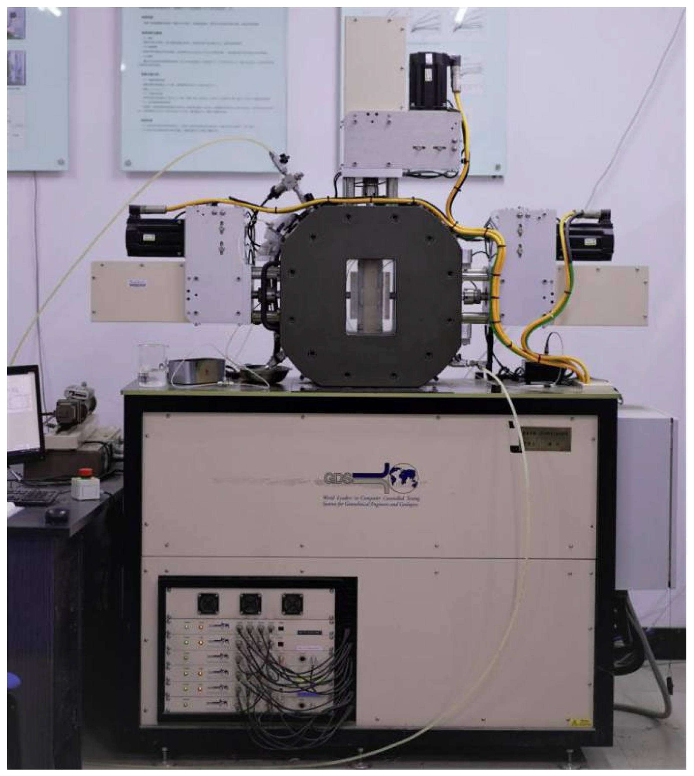
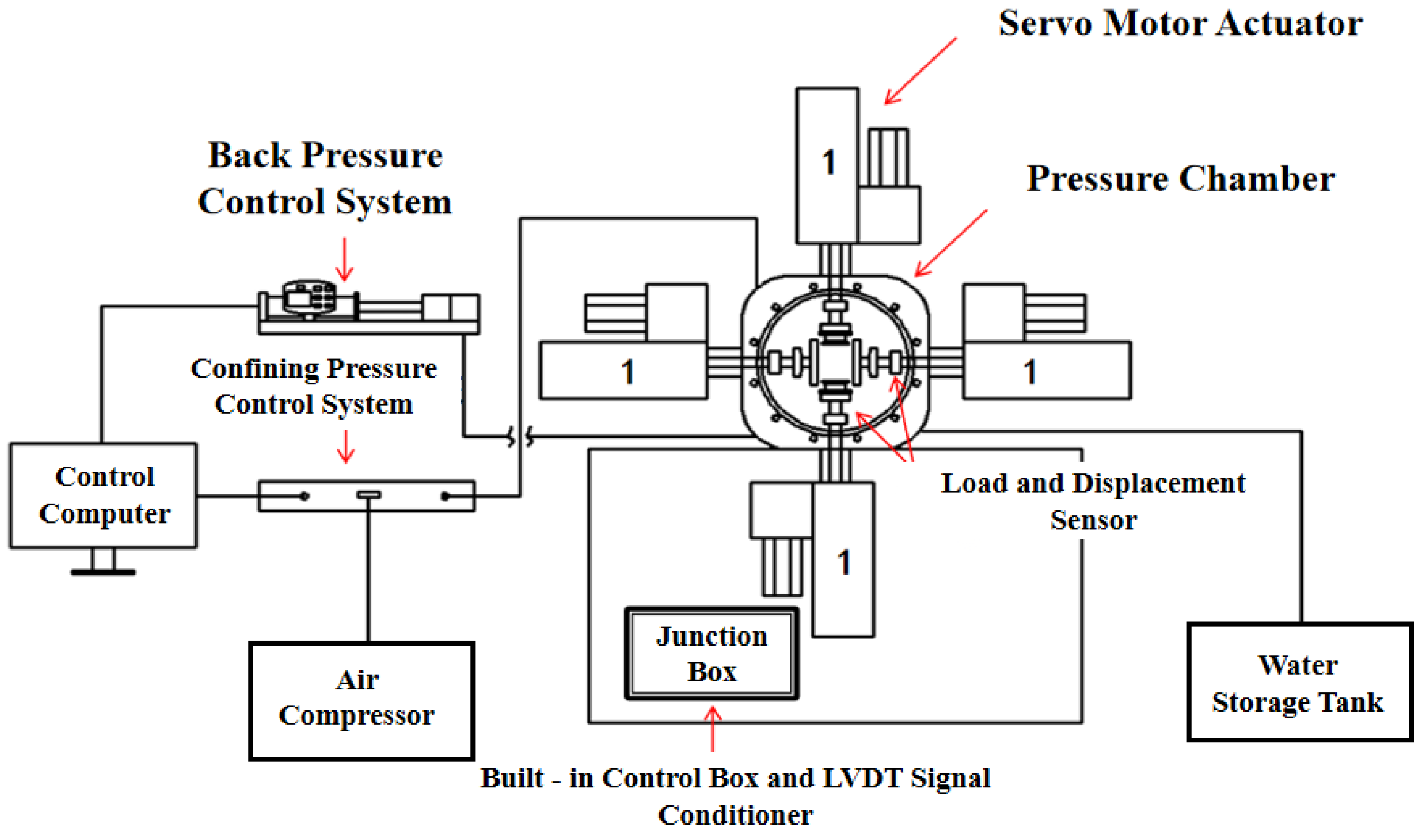
The experimental research in this study was conducted using a GDS dynamic and static true triaxial apparatus (EMTTA), as illustrated in Figure 1 and Figure 2. This advanced equipment comprises several key components, including a pressure chamber, servo motor actuator, confining pressure control system, and backpressure control system. Additionally, it is equipped with load and displacement sensors, a built-in control box integrated with a Linear Variable Differential Transformer (LVDT) signal conditioner, and a water storage tank. The apparatus is controlled and monitored via a dedicated computer system using GDSLAB control and data acquisition software, ensuring precise and reliable measurements throughout the experiments.

2.2. Experimental Materials and Sample Preparation

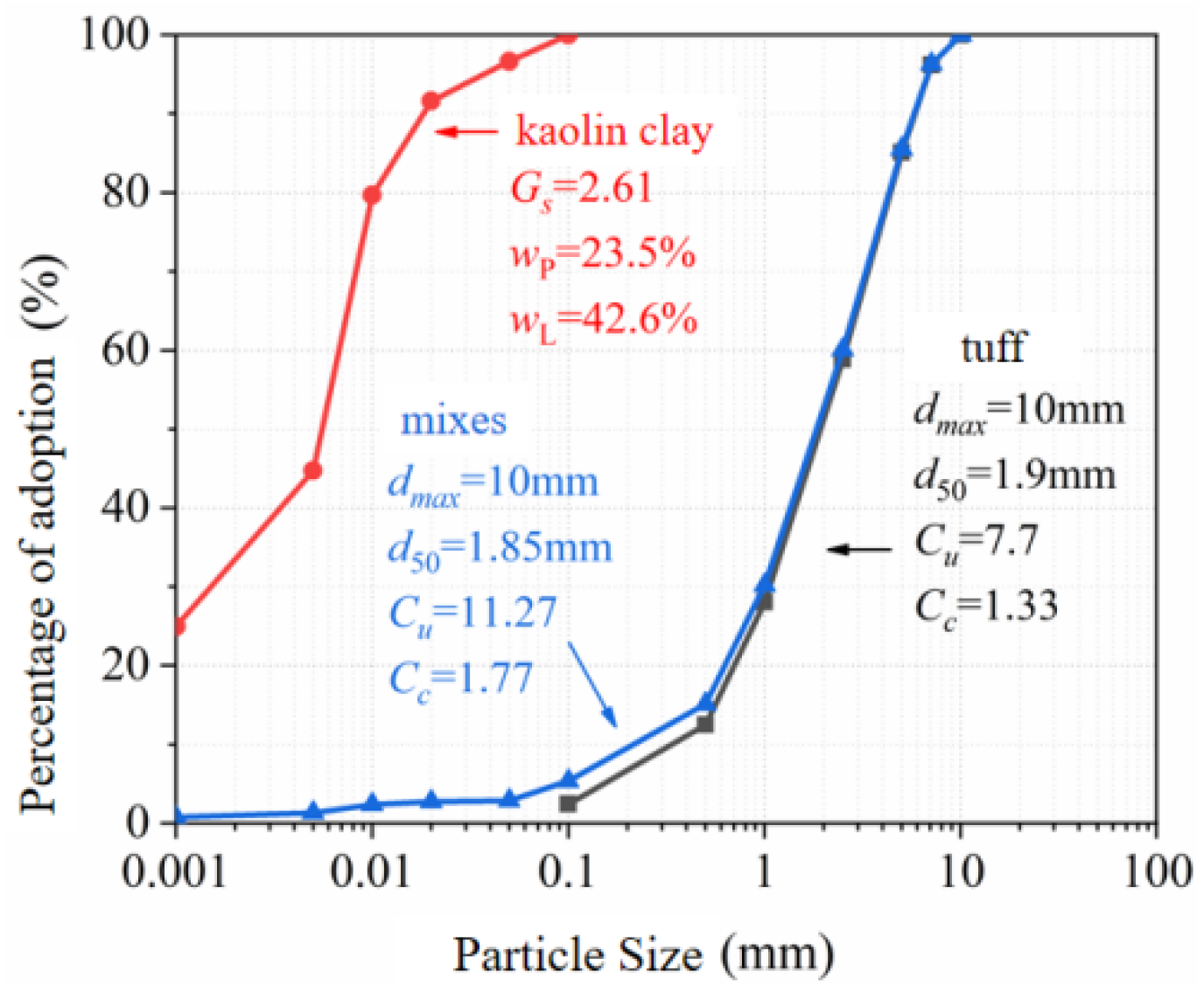
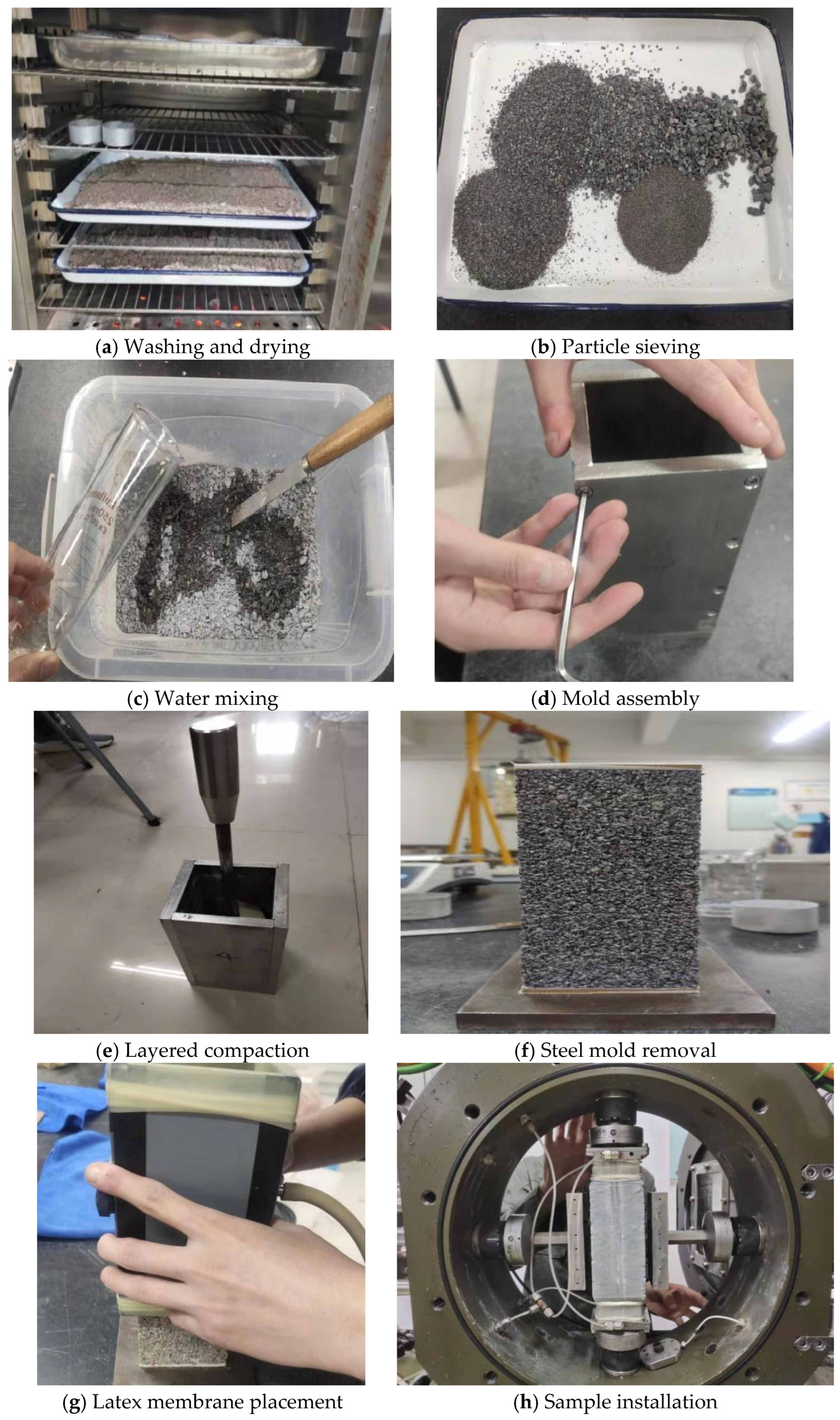
The experimental material used in this study was tuff gravel obtained from a quarry near Wenzhou. After washing, drying, and sieving, the material was divided into six particle groups, as shown in Figure 3. Considering the construction conditions and seasonal fluctuations in groundwater levels, a 3% fine content was incorporated into the samples by mixing 3% (by dry weight) of kaolinite with the tuff gravel. The gradation curve of the tuff mixture (Figure 3) met the requirements for coarse-grained soils specified in the Highway Subgrade Design Code. Based on the Standards for Soil Testing Methods, the maximum dry density and optimum water content of the tuff mixture were determined to be 2.14 g/cm3 and 8%, respectively.
The true triaxial samples used in this study were rectangular specimens with dimensions of 75 mm × 75 mm × 160 mm. The preparation process required various tools and materials, including a detachable four-part steel mold, a removable membrane holder, a compaction hammer, a vacuum pump, latex membranes, metal porous stones, and permeable non-woven fabrics.
The samples were prepared using the layered compaction method, with six layers compacted to achieve a compaction degree of over 95%, meeting the requirements for coarse-grained soils specified in the Highway Subgrade Design Code for subgrade and pavement base/subbase layers. The preparation process is illustrated in Figure 4.
This study considered two moisture conditions: an optimum water content to simulate ideal working conditions and a saturated state to represent extreme scenarios, such as heavy rainfall.
For the saturated samples, a saturation process was performed prior to the shear or cyclic loading tests. First, a confining pressure of 20 kPa was applied to the sample, and CO2 gas was introduced from the bottom of the sample through the backpressure channel for 0.5 h to displace air within the sample. Next, the GDS standard pressure/volume controller (STDDPC V2) was connected to the backpressure channel, and de-aired water was introduced from the bottom until the water flow stabilized. Finally, the effective confining pressure was maintained at 20 kPa, and the backpressure was increased to 200 kPa to dissolve residual CO2. The sample was considered saturated when the drainage volume change rate was less than 200 mm3/h, and the b-value (measured using the b-check pore pressure parameter monitoring module) exceeded 0.98.

2.3. Stress State and Its Characterization Parameters

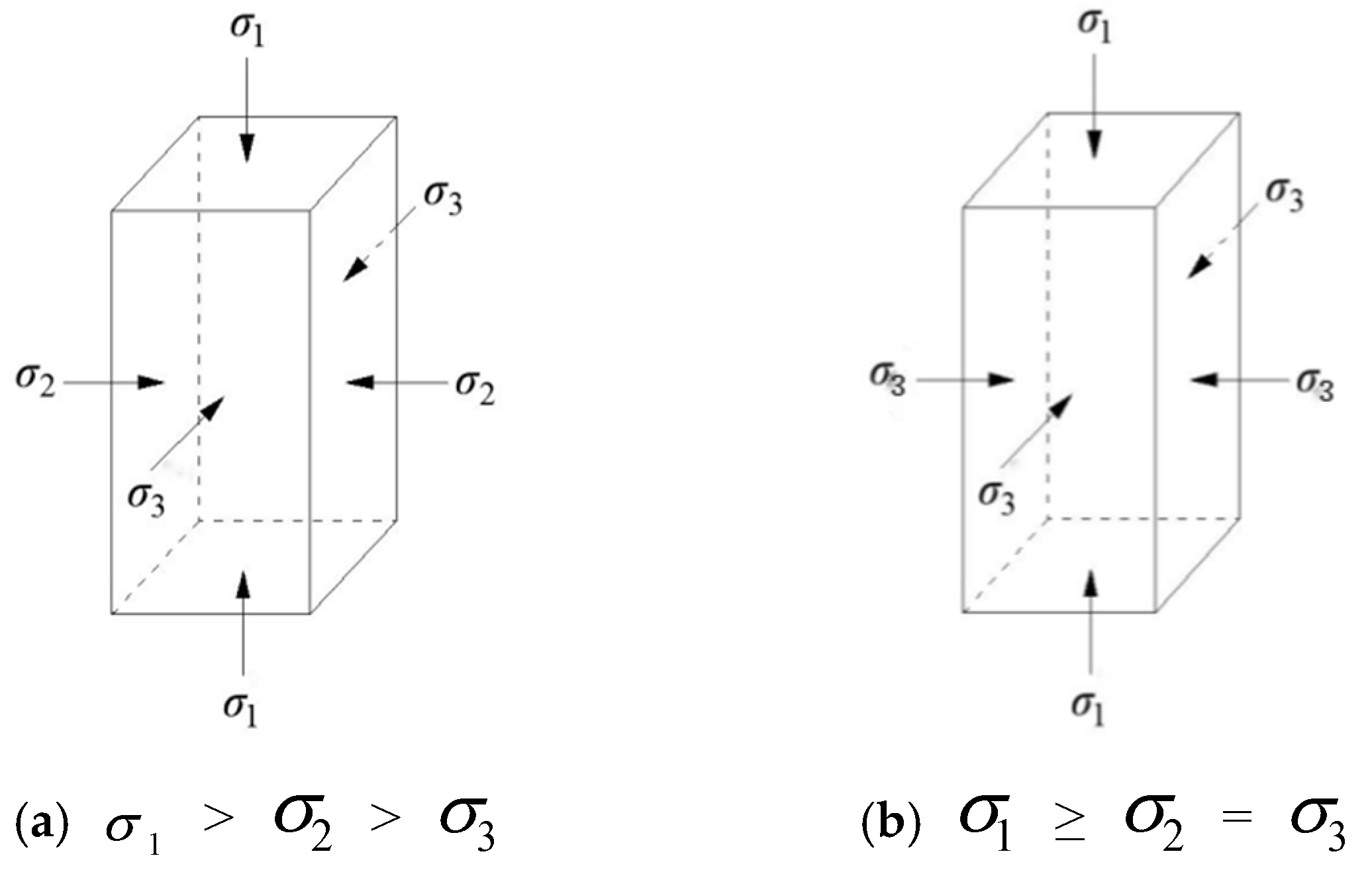
The stress state of a sample includes the initial stress state. Under three-dimensional stress conditions, the initial stress state (Figure 5a,b) can be characterized by three parameters: the initial mean principal stress (p0), the initial generalized shear stress (qini), and the initial intermediate principal stress coefficient (bini). The relationships between the initial major principal stress, intermediate principal stress, minor principal stress, and these three parameters are expressed in Equations (4)–(6).
p 0 = 1 3 ( σ 1 + σ 2 + σ 3 )
q i n i = 2 2 ( σ 1 σ 2 ) 2 + ( σ 1 σ 3 ) 2 + ( σ 2 σ 3 ) 2
b i n i = σ 2 σ 3 σ 1 σ 3
σ 1 = p 0 + q i n i ( 2 b i n i ) 3 1 b i n i + ( b i n i ) 2
σ 2 = p 0 + q i n i ( 2 b i n i 1 ) 3 1 b i n i + ( b i n i ) 2
σ 3 = p 0 q i n i ( 1 + b i n i ) 3 1 b i n i + ( b i n i ) 2
On the π-plane, all points share the same mean principal stress (p). The stress Lode angle (θ) is commonly used to reflect the direction of generalized shear stress under three-dimensional stress conditions. Its relationship with the intermediate principal stress coefficient (b) is defined by Equation (7). Therefore, the direction of the generalized shear stress in a three-dimensional state can be described using b. Table 1 lists the corresponding stress Lode angles (θ) for the different values of b used in this study.
tan θ = 2 σ 2 σ 1 σ 3 3 ( σ 1 σ 3 ) = 2 b 1 3

2.4. Test Plan

2.4.1. Static Shear Test Plan for Coarse-Grained Soil Under Initial Isotropic Stress Conditions

A total of 11 static shear tests were conducted on coarse-grained soil with saturated and optimum water content conditions under low confining pressures ( σ 3 = 20 kPa, 30 kPa, 40 kPa, 60 kPa). The initial stress state of the samples was isotropic. The tests included 4 drained tests at optimum water content, 4 drained tests under saturated conditions, and 3 undrained tests under saturated conditions. The detailed test plan is shown in Table 2.
The tests applied axial stress (major principal stress) in a strain-controlled mode, with a shear rate of 0.2%/min. Due to equipment limitations, the maximum axial strain (major principal stress direction) was set at 12%, corresponding to a maximum loading time of 60 min.

2.4.2. Static Shear Test Plan for Coarse-Grained Soil Under Three-Dimensional Initial Anisotropic Stress Conditions

To investigate the shear characteristics of coarse-grained soil under three-dimensional initial anisotropic stress conditions, the initial stress state was characterized using the initial mean principal stress (p0), initial generalized shear stress (qini), and initial intermediate principal stress coefficient (bini). Considering practical conditions in foundation engineering, a total of 27 true triaxial static shear tests were conducted, with the detailed test plan shown in Table 3.
All tests were performed under drained conditions. Axial stress (major principal stress) was applied in a strain-controlled manner, with a shear rate of 0.2%/min. Due to equipment limitations, the maximum axial strain (major principal stress direction) was set at 12%, corresponding to a maximum loading time of 60 min.

2.4.3. Static Shear Test Plan for Coarse-Grained Soil Under Plane Strain Conditions

To study the shear characteristics of coarse-grained soil under plane strain conditions, 6 static shear tests were conducted on saturated and optimum water content coarse-grained soil under low confining pressures ( σ 3 = 20 kPa, 30 kPa, 40 kPa). The detailed test plan is shown in Table 4.
All tests were performed under drained conditions. Axial stress (major principal stress) was applied in a strain-controlled manner, with a shear rate of 0.2%/min. Due to equipment limitations, the maximum axial deformation (major principal stress direction) in this set of tests was set at 12%, corresponding to a maximum loading time of 60 min.

3. Test Results

3.1. Static Shear Test Results and Analysis for Coarse-Grained Soil Under Initial Isotropic Stress Conditions

3.1.1. Stress–Strain Relationship and Strength

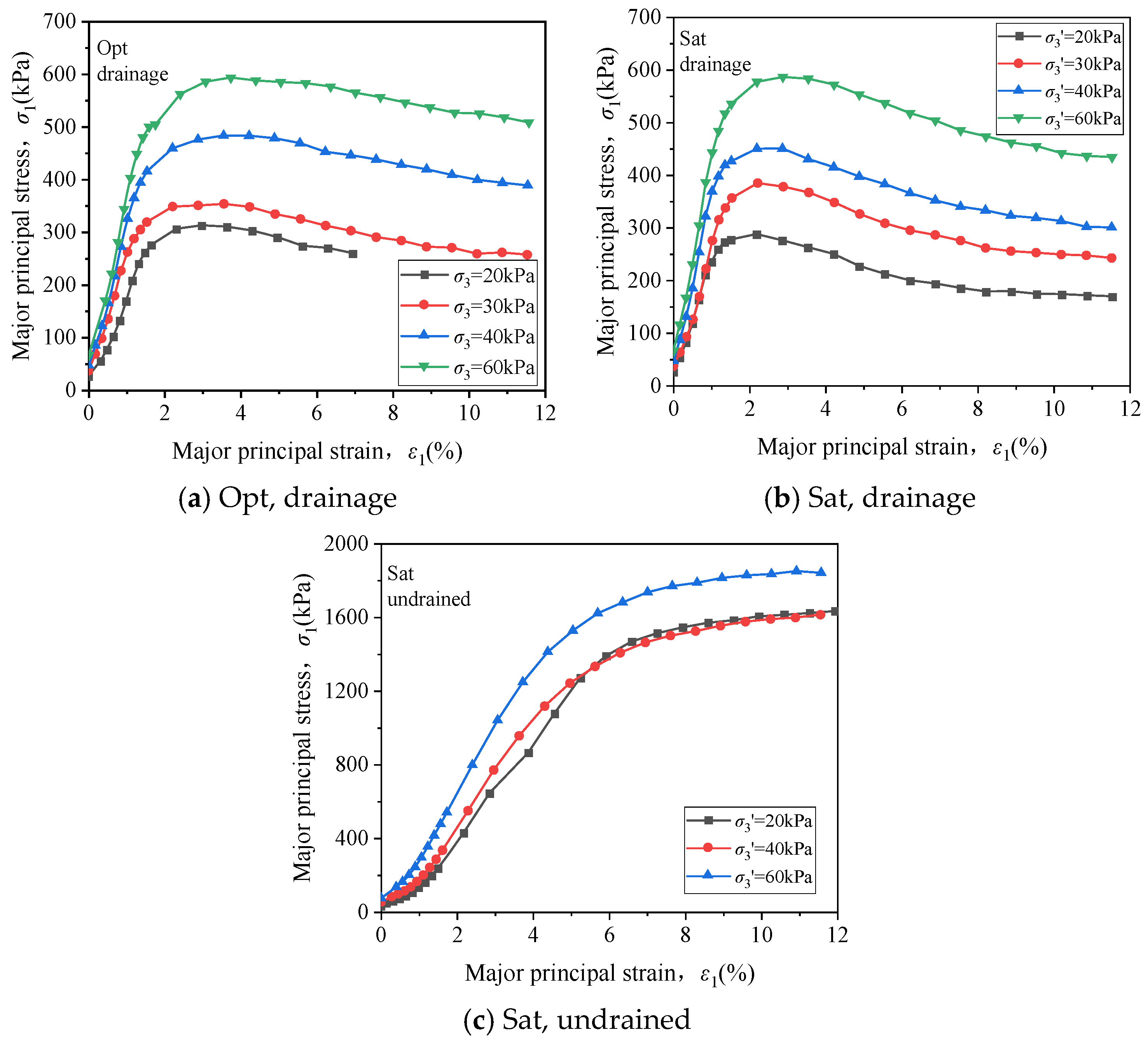
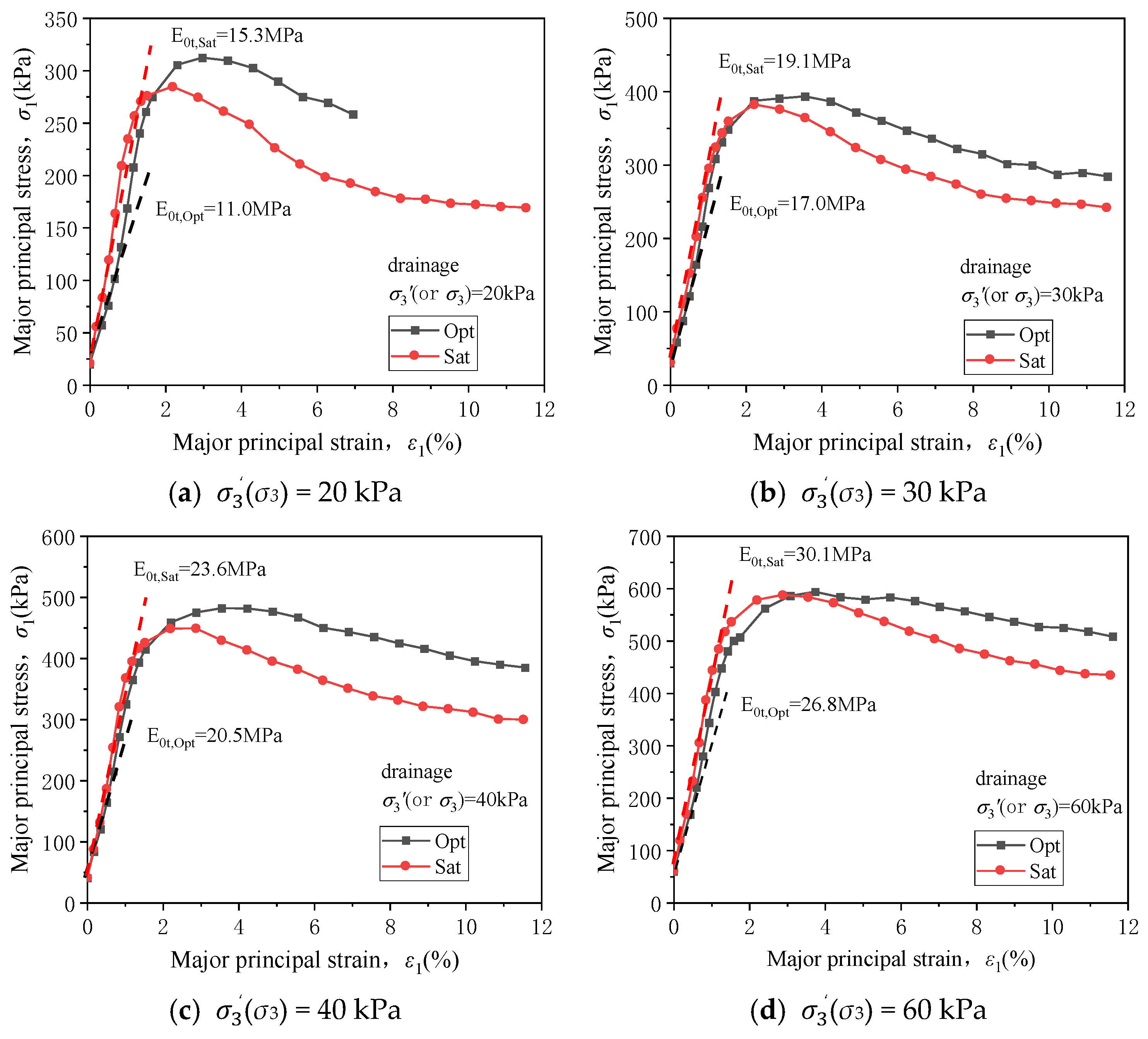
Figure 6 summarizes the major principal stress–major principal strain curves for the 11 tests discussed in this section. Under drained conditions (Figure 6a,b), all the samples exhibit strain-softening behavior: the major principal stress increases rapidly with increasing strain at the initial phase of loading, reaches a peak, and then gradually decreases. For the coarse-grained soil with the optimum water content (Figure 6a), the major principal stress does not stabilize within the tested strain range. For the saturated samples (Figure 6b), the major principal stress tends to stabilize after the major principal strain exceeds 12%, indicating that the soil approaches a critical state. Under the undrained conditions (Figure 6c), the stress–strain curves exhibit strain-hardening behavior, with the major principal stress stabilizing after the strain exceeds 6%.
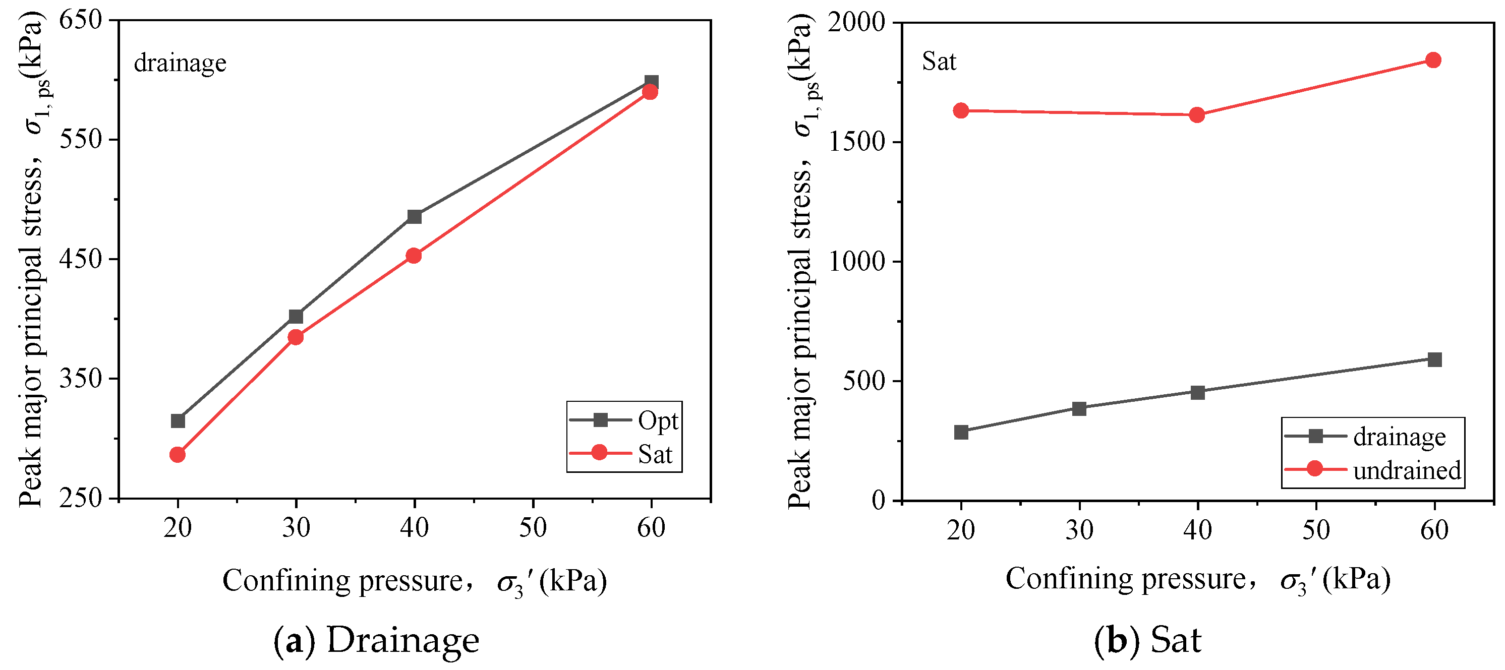
The stress–strain relationships show that increasing the confining pressure significantly enhances the shear strength, including both peak and residual values, which is clearly observed in Figure 6a,b. Figure 7a further demonstrates that the peak major principal stress increases nearly linearly with the confining pressure under both water conditions. By comparison, the peak major principal stress under optimum water content is slightly higher than under saturated conditions, with the differences generally within 10%. For instance, at a confining pressure of σ 3 = 40 kPa, the peak major principal stress is 485.6 kPa under optimum water content, compared to 452.4 kPa under saturated conditions. The strain corresponding to the peak stress (peak strain) is also larger under optimum water content. For the same confining pressure, the peak strain is approximately 3.1% for optimum water content and 2.5% for saturated conditions.
Comparing Figure 6b,c, and observing Figure 7b, it is evident that under saturated conditions, the strain-softening behavior in drained conditions and the strain-hardening behavior in undrained conditions reflect different work-hardening mechanisms. If the major principal stress at the end of the undrained test is considered the peak stress, it is significantly higher than the peak stress under drained conditions, approximately 3.1 to 5.7 times greater.

3.1.2. Modulus

The initial tangent modulus (E0t) and the secant modulus (E50, at 50% of the peak strength) are key parameters reflecting soil stiffness. The initial tangent modulus is calculated assuming elastic behavior within a strain range of 0.1%. The secant modulus is defined as the slope of the line connecting the origin to the point at 50% peak stress, expressed in Equation (8).
E 50 = 0.5 Δ σ 1 ,   max ε 1 , 0.5 Δ σ 1 ,   ps
In this context, Δ σ 1 , max max represents the maximum change in the major principal stress, while ε 1 , 0.5 Δ σ 1 , ps corresponds to the major principal strain at 50% of the maximum change in the major principal stress.
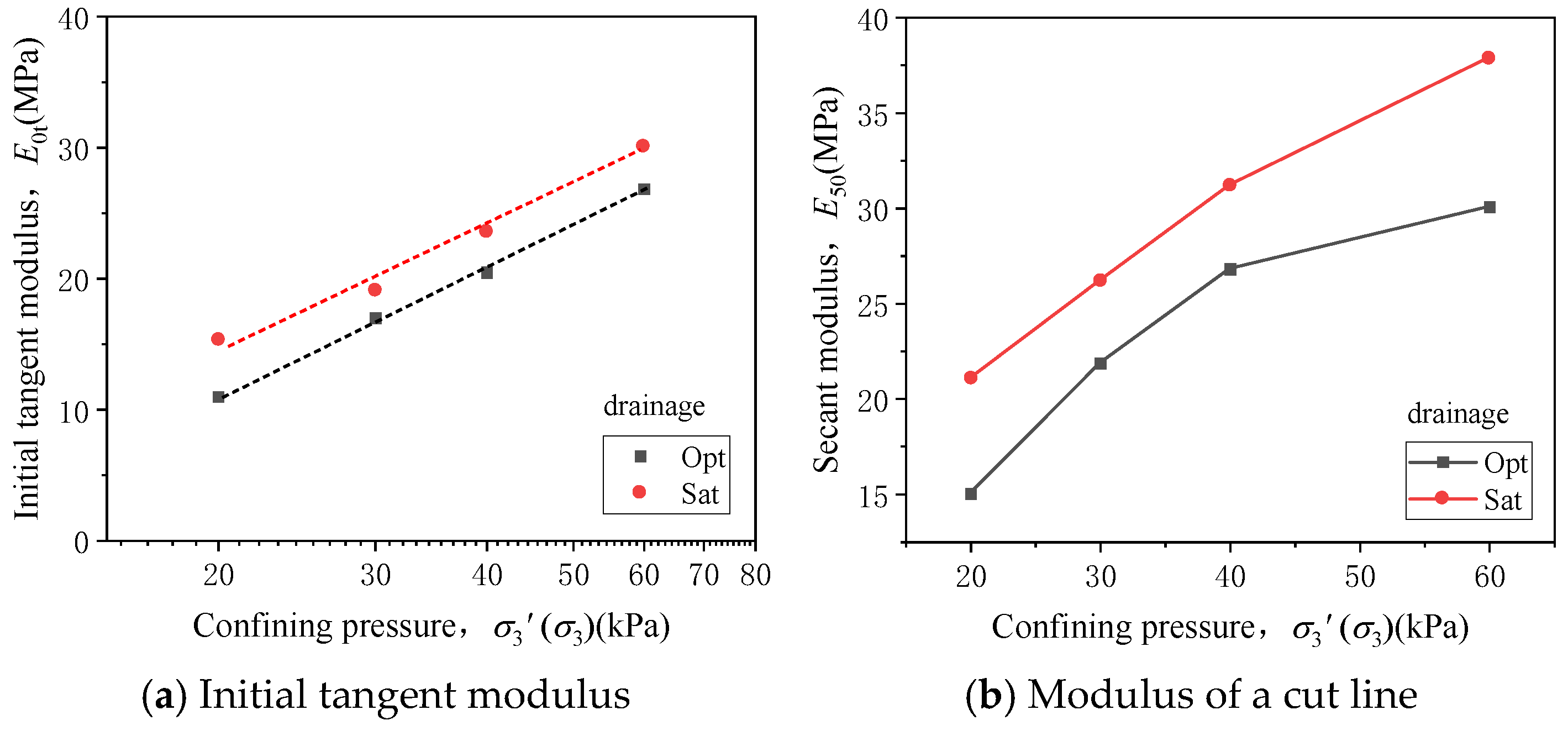
Figure 8a–d compares the stress–strain relationships for the saturated and optimum water content samples under the same confining pressure in the drained tests. The saturated samples exhibit faster stress increases and earlier peak strengths, with a higher initial tangent modulus (E0t). The difference in the E0t ranges from 2.1 to 4.3 MPa, or 12.3% to 39.7%.
Figure 9a shows that E0t increases with the confining pressure, following a linear relationship on a logarithmic scale (lg σ 3 ).
E 0 t = a + m lg σ 3
For this equation, under optimum water content and drained conditions, a1 = −31.78, m1 = 32.86; under saturated and drained conditions, a2 = −26.20, m2 = 31.33.
Figure 9b compares the E50- σ 3 (σ3) relationships under saturated and optimum water content conditions. The secant modulus E50 increases with the confining pressure and shows a linear relationship within the range of 20 kPa ≤ σ 3 ≤ 40 kPa. Similar to the initial tangent modulus, E50 is higher under saturated conditions, with differences of 6.0–7.8 MPa (16.4–40.2%).
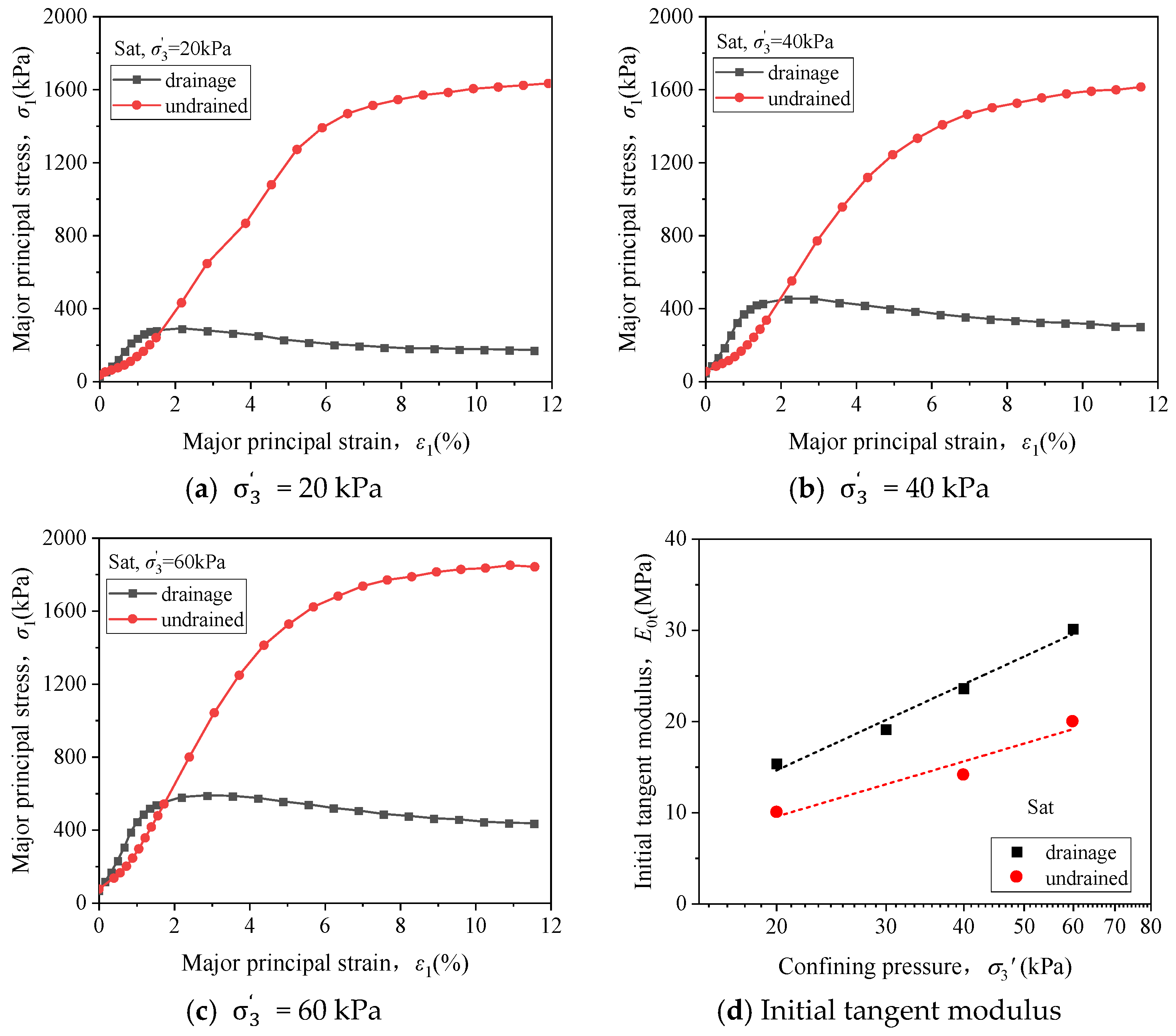
Figure 10a–c compares the stress–strain relationships under different drainage conditions, with the initial tangent modulus comparisons shown in Figure 10d. Although the peak major principal stress is much higher under undrained conditions, the initial tangent modulus is lower than that for drained conditions, with percentage differences of 50.9–67.3%. This is because positive excess pore pressure at the start reduces the effective confining pressure, lowering the soil stiffness. In the later stages, negative excess pore pressure increases the effective confining pressure, enhancing the soil strength.

3.1.3. Friction Angle

The friction angle is one of the key strength parameters of soil, influenced by factors such as particle gradation, particle shape, water content, and changes in the stress state. In triaxial shear tests, the relationship between the friction angle φ and the stress ratio η can be expressed by Equation (10).
sin φ = 3 η 6 + η ,   included   among   these   η = q p
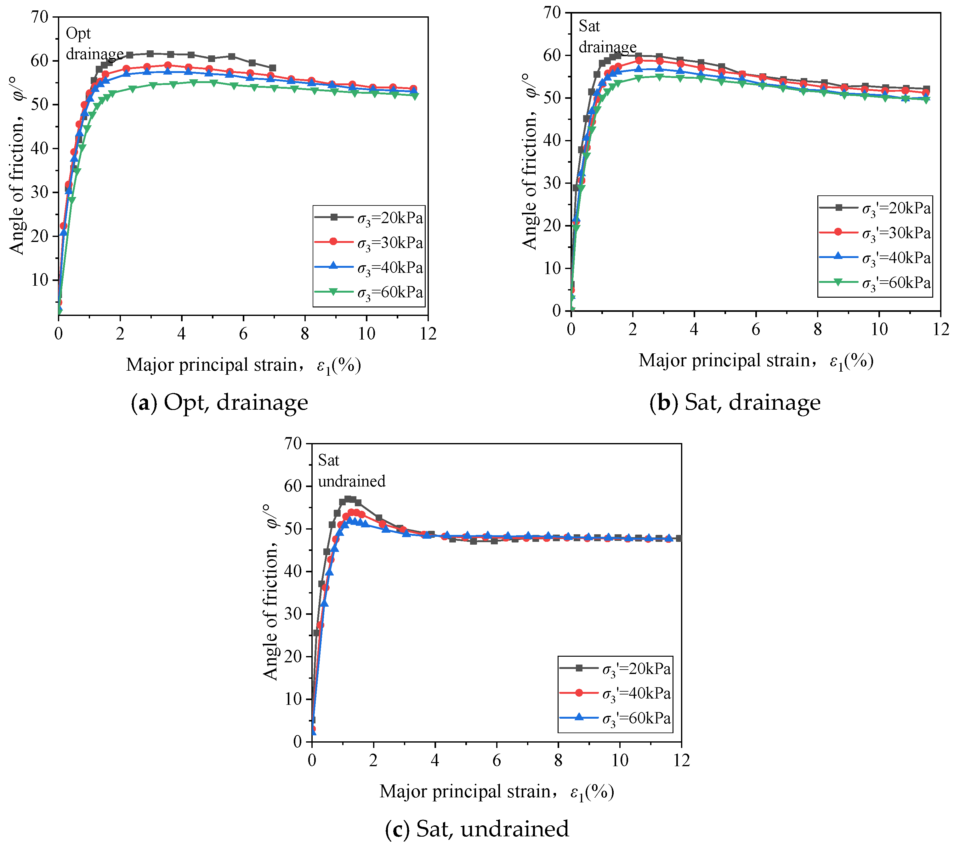
Figure 11 shows the variation in the friction angle φ with the major principal strain ε1. Under different water contents and drainage conditions, the φ-ε1 relationships are similar: φ increases rapidly with ε1 during the initial loading stage. Under drained conditions, it reaches a peak friction angle φps at the peak strain, then gradually decreases and stabilizes. In undrained conditions, the peak friction angle of coarse-grained soils does not occur at the peak stress but stabilizes rapidly during the later stages of the test.
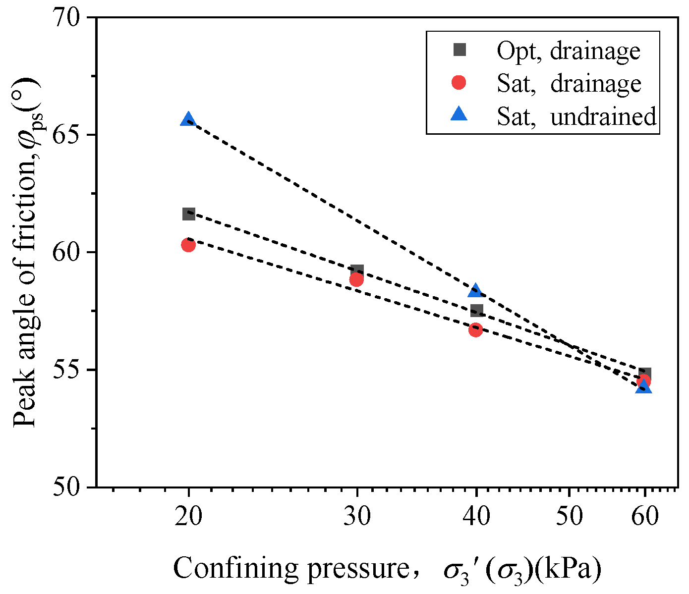
To analyze the relationship between the friction angle of coarse-grained soil and the confining pressure, Figure 12 presents the curve of the peak friction angle φps versus the logarithmic value of confining pressure lg σ 3 . It shows a strong linear relationship in all three cases, where φps decreases linearly as lg increases. The relationship can be expressed by the following equation:
φ = c + n lg σ 3
In the equation, under optimum water content and drained conditions, c1 = 80.18, n1 = −14.2; under saturated drained conditions, c2 = 76.85, n2 = −12.54; and under saturated undrained conditions, c3 = 96.79, n3 = −24.00.
It can also be observed that under drained conditions, the peak friction angle of saturated samples is slightly lower than that of optimum water content samples. At confining pressures of 20, 30, 40, and 60 kPa, the peak friction angles for the optimum water content are 61.6°, 59.2°, 57.5°, and 54.8°, respectively, while for the saturated samples they are 60.3°, 58.8°, 56.6°, and 54.5°, with differences of 1.3%, 0.4%, 0.9%, and 0.3%. Studies suggest that as the water content increases, the soil pore spaces are gradually filled with water, and the lubricating effect of water reduces the interparticle friction, lowering the friction angle. However, once the water content reaches a certain level, the contact points between particles are fully covered by water films, and further increases in the water content have a minimal impact on the friction angle. Comparing the drained and undrained test results of saturated samples reveals that as the confining pressure increases, the difference between the two conditions decreases, with the peak friction angle under undrained conditions decreasing more rapidly, indicating that the confining pressure has a stronger effect on the peak friction angle under undrained conditions.

3.1.4. Stress Ratio

The stress ratio η is defined as the ratio of generalized shear stress q to the mean principal stress p during shearing. Compared with the generalized shear stress, it normalizes the influence of mean principal stress. The specific calculation formula is given in Equation (12). Notably, the peak stress ratio η f is particularly useful for characterizing a soil’s ability to resist external loads. A larger η f indicates stronger resistance to deformation and greater strength under the unit mean principal stress, while a smaller η f indicates the opposite.
η = q p
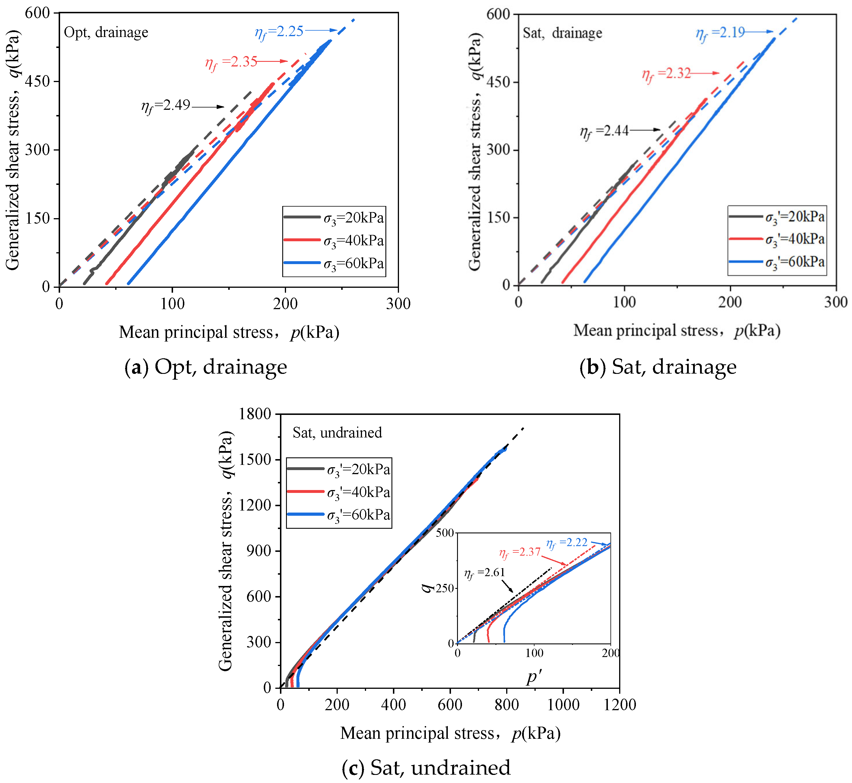
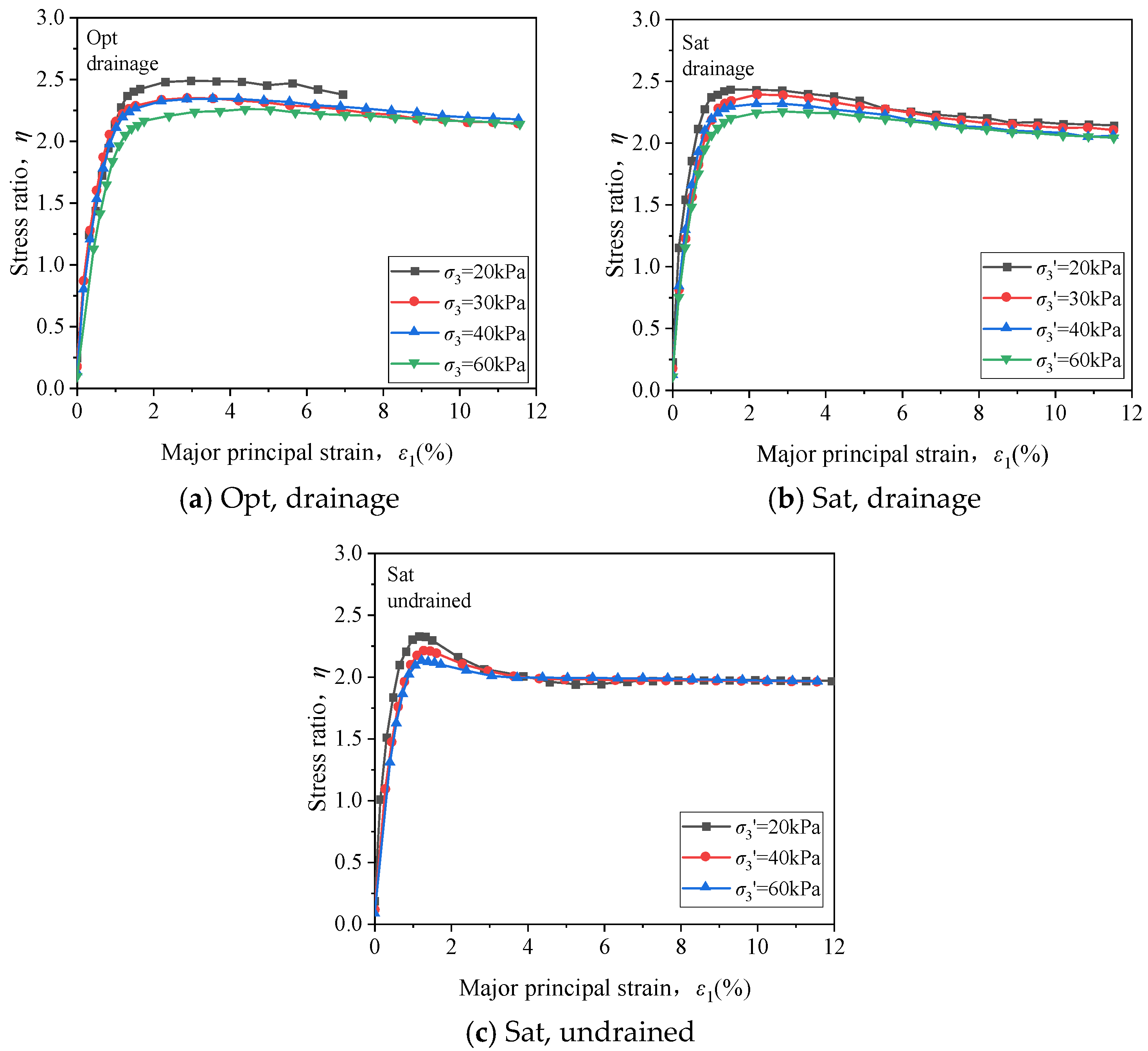
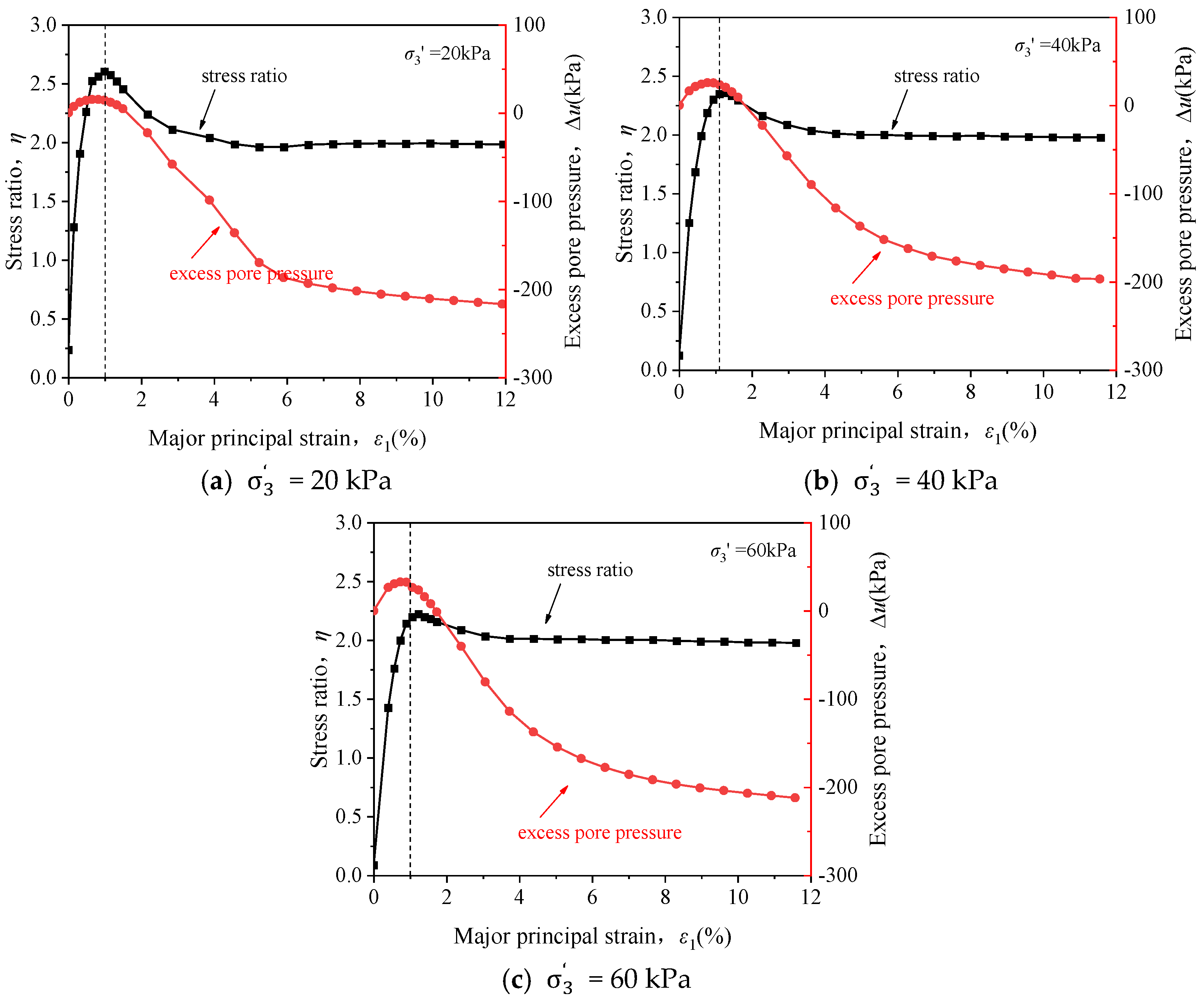
Figure 13 shows the variation in the stress ratio η with the major principal strain ε1 under different confining pressures. Comparing this with Figure 6, under drained conditions, both the major principal stress–strain and stress ratio–strain relationships exhibit weak strain-softening behavior. In contrast, under undrained conditions, the stress–strain relationship shows strain hardening, while the stress ratio–strain relationship exhibits strain softening. To analyze this phenomenon, Figure 14 presents the stress paths under confining pressures of 20, 40, and 60 kPa, where the stress ratio corresponds to the slope of the line connecting any point on the stress path to the origin. The dashed line represents the slope of the line from the origin to the point of peak generalized shear stress, which indicates the peak stress ratio under drained conditions. Figure 14c shows that under undrained conditions, parts of the stress path lie above the dashed line, meaning the peak stress ratio does not occur at the peak generalized shear stress. Figure 3, Figure 4, Figure 5, Figure 6, Figure 7, Figure 8, Figure 9 and Figure 10 further illustrate the relationships between the excess pore pressure, stress ratio, and major principal strain under undrained conditions.
According to the effective stress principle in soil mechanics, the total stress in saturated soil is shared by the soil skeleton and pore water. Since pore water is incompressible and drainage is closed, positive excess pore pressure is generated during initial loading (Figure 15), reducing the effective confining pressure and causing the effective mean stress to increase slowly (Figure 14c), which leads to a rapid increase in the stress ratio. As the excess pore pressure transitions from positive to negative, the effective confining pressure increases, the effective mean stress rises rapidly, and the stress path bends, causing the stress ratio to decrease quickly to a stable value. This explains why the peak stress ratio under undrained conditions does not coincide with the peak generalized shear stress (Figure 14c), resulting in strain-softening behavior in the stress ratio–strain relationship.
Figure 13 shows that the development of the stress ratio η aligns closely with the friction angle (Figure 11). Comparisons between the curves indicate that the confining pressure has a minimal effect on η, especially in the later stages of testing. Although η decreases slightly with an increasing confining pressure, the change is negligible, contrasting significantly with the stress–strain relationship in Figure 6.
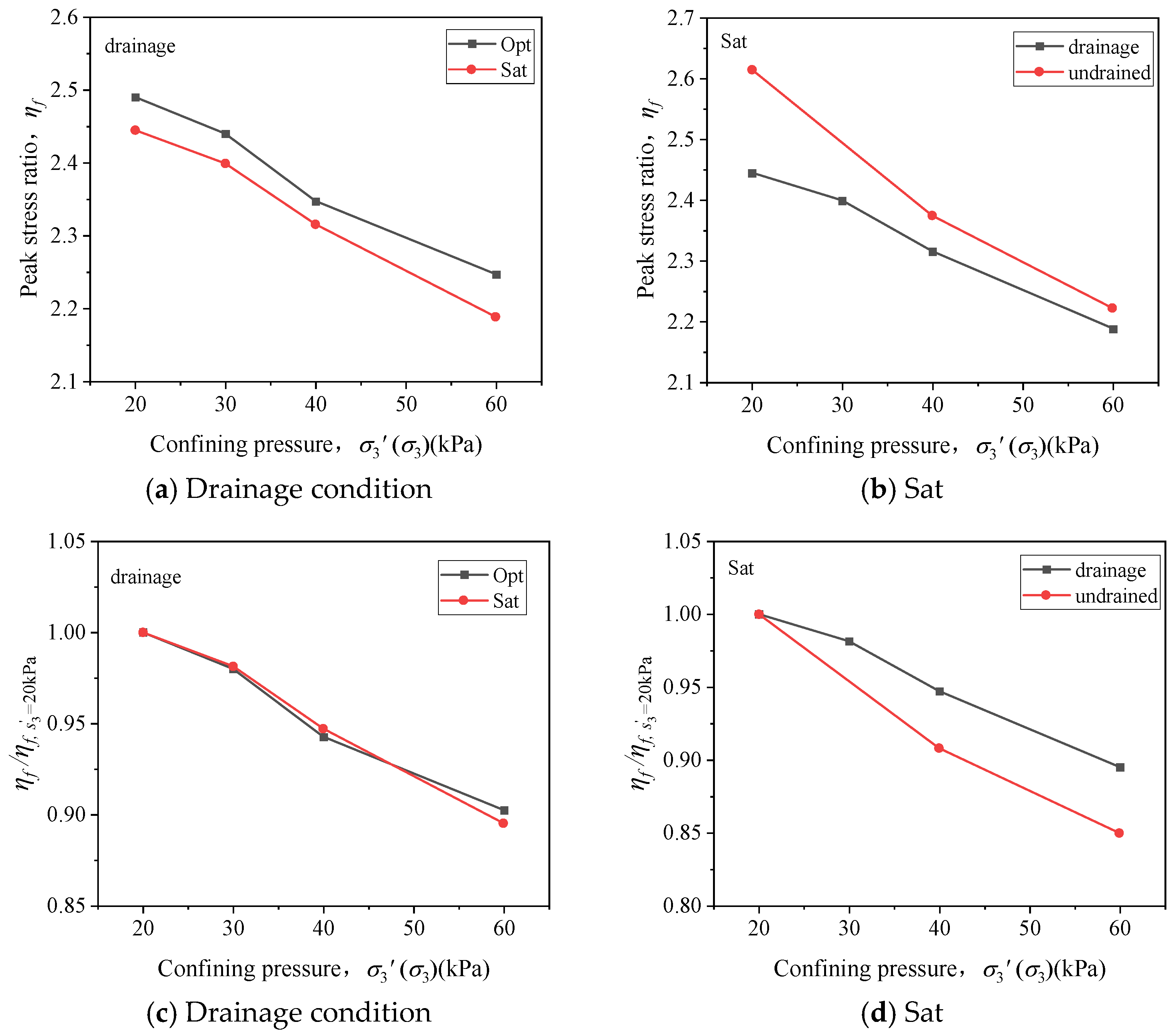
To further analyze the relationship between the peak stress ratio η f and confining pressure, Figure 16 shows the curves of η f and its normalized values with the confining pressure. Under different water contents and drainage conditions, η f decreases approximately linearly with an increasing confining pressure. In drained conditions (Figure 16a), the peak stress ratio of the optimum water content samples is slightly higher than that of saturated samples, with differences of 0.05, 0.04, 0.03, and 0.06 at confining pressures of 20, 30, 40, and 60 kPa, respectively. These differences, ranging from 1.29% to 2.74%, indicate the limited influence of water content on η f .
Figure 16c shows that the normalized curves for the saturated and optimum water content samples are nearly identical, suggesting the water content has no effect on the normalized η f –confining pressure relationship. Under different drainage conditions (Figure 16c), η f is higher in undrained conditions than in drained conditions. Figure 16d indicates that as the confining pressure increases, η f decreases more rapidly under undrained conditions, and the difference between the drainage conditions gradually diminishes, showing that the influence of drainage conditions on the η f –confining pressure relationship weakens with an increasing confining pressure.

3.2. Triaxial Initial Anisotropic Stress State: Static Shear Characteristics of Coarse-Grained Soil

3.2.1. Stress–Strain Relationship and Strength

In all the shear tests in this section, the major principal stress gradually increases, while the intermediate and minor principal stresses remain constant. Therefore, the focus is on the major principal stress–major principal strain relationship, with some analyses also based on generalized shear stress–generalized shear strain relationships.
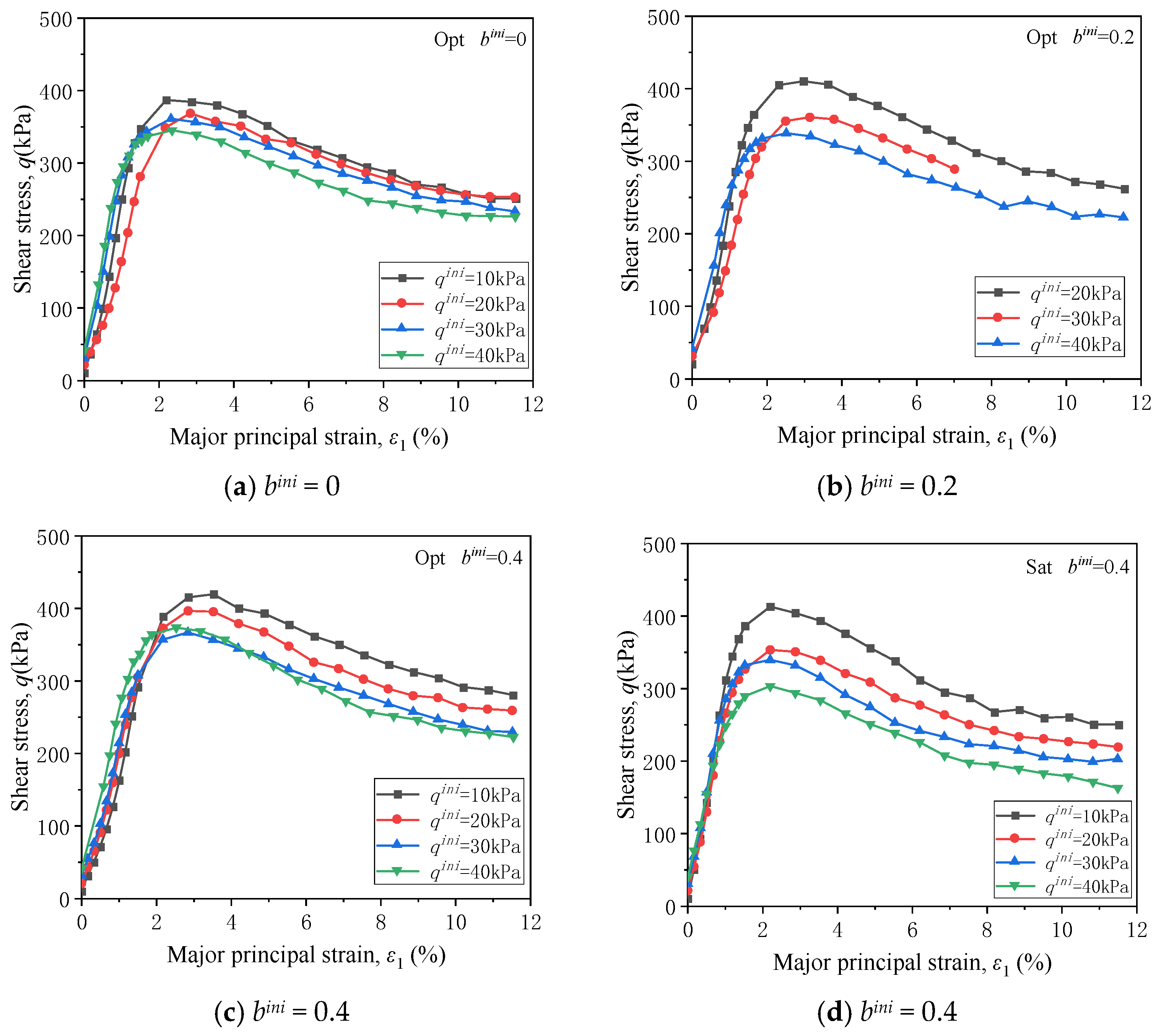
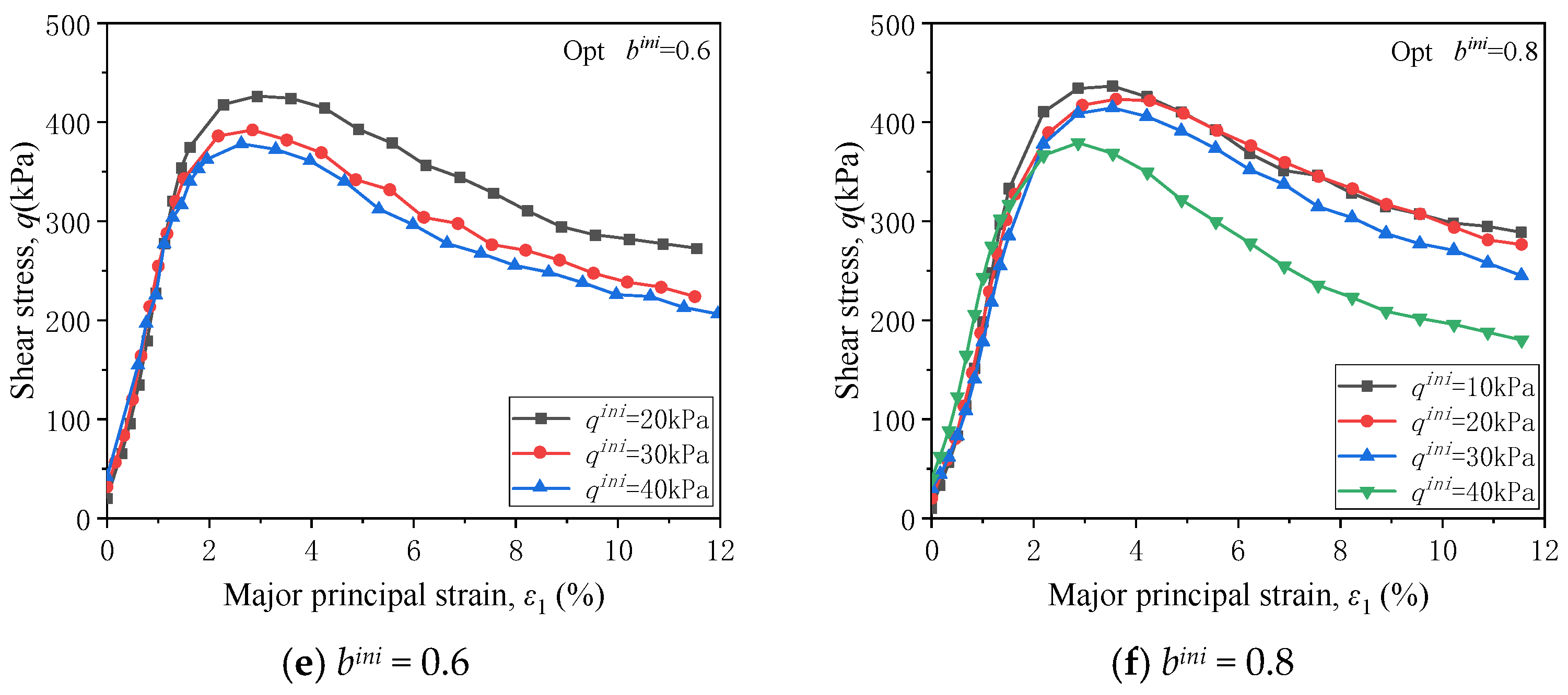
Figure 17 shows the major principal stress–major principal strain curves under triaxial initial anisotropic stress conditions. All the specimens exhibited significant strain-softening behavior, where the major principal stress increased gradually from the start of loading, reached a peak at 2–4% major principal strain, and then decreased slowly, and stabilized at a constant value. Due to the displacement range limitation of the testing equipment, most specimens did not reach the critical state when the major principal strain reached about 12%.
The peak strength of coarse-grained soil at optimum water content ranges from 365.9 to 477.4 kPa. Comparing the test results under the different initial generalized shear stresses in each graph shows that an increase in the initial generalized shear stress causes a decrease in the peak major principal stress and also affects the major principal strain corresponding to the peak stress. Furthermore, based on the trends in the stress–strain curves, higher initial generalized shear stresses result in lower critical major principal stresses.
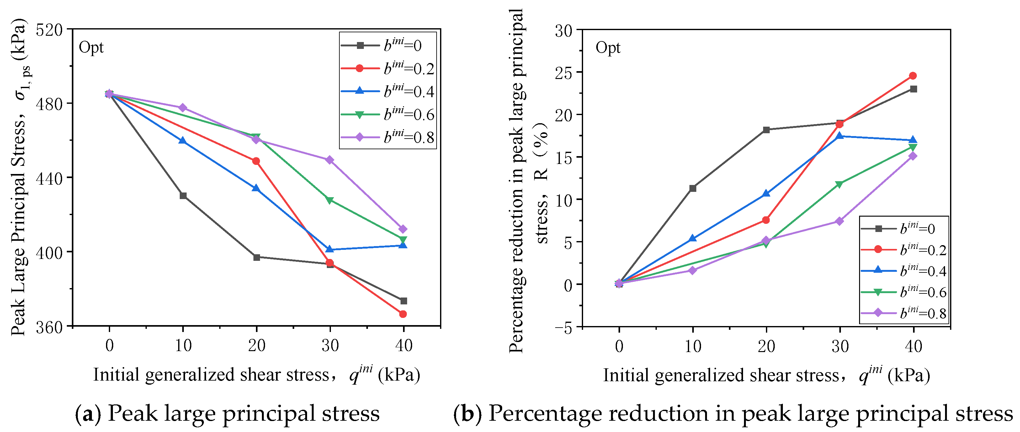
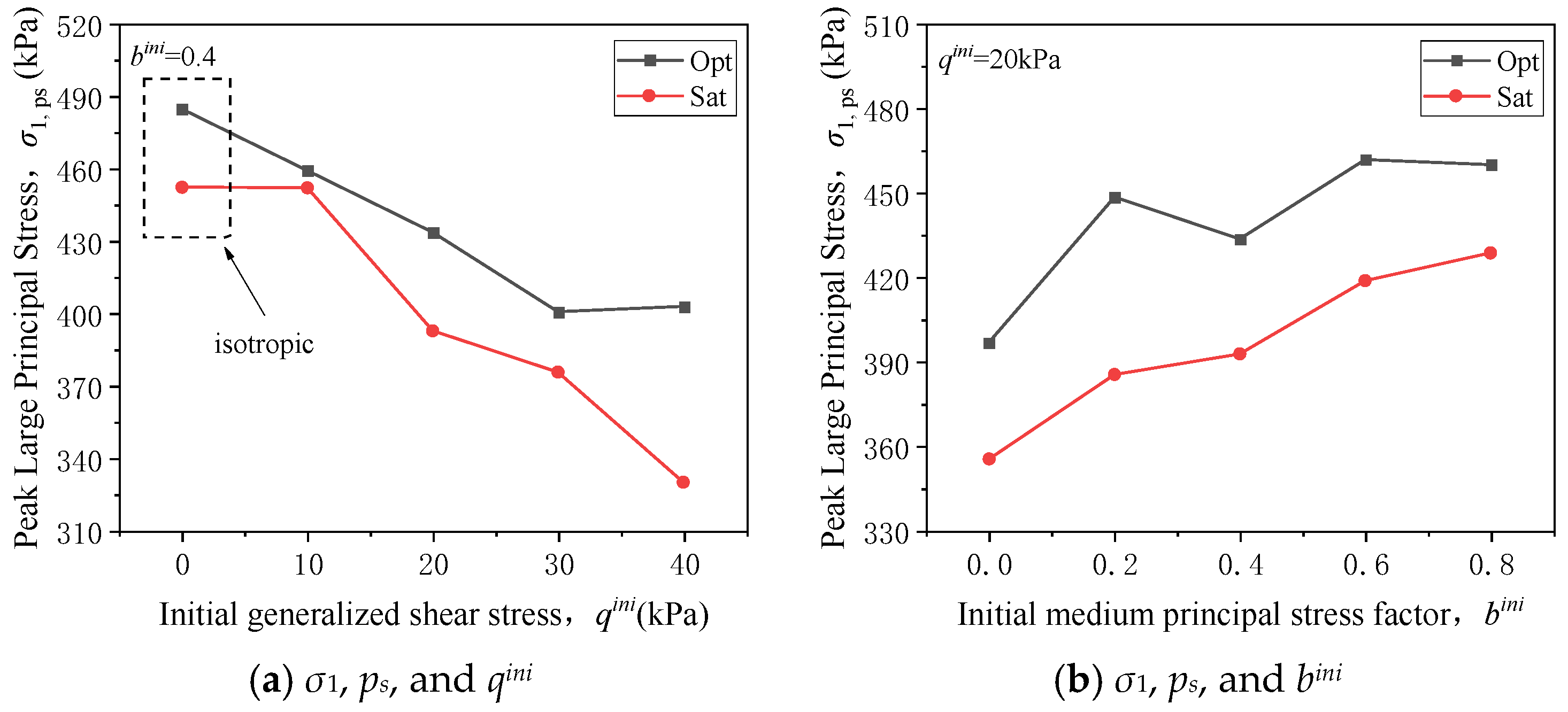
To further analyze the influence of initial generalized shear stress qini on the peak major principal stress, Figure 18a illustrates the relationship between the peak major principal stress and qini for coarse-grained soil at optimum water content under different bini values. It is evident that as qini increases, the peak major principal stress decreases significantly.
Taking bini = 0.8 as an example, the peak major principal stresses at qini = 10, 20, 30, and 40 kPa are 477.4, 460.1, 449.2, and 411.8 kPa, respectively. Compared to the initial isotropic state (qini = 0, bini = 0), the decreases are 1.5%, 5.1%, 7.3%, and 15.1% at qini = 10, 20, 30, and 40 kPa, respectively.
Using the peak major principal stress under the initial isotropic state (qini = 0, bini = 0) as a reference, the percentage reduction in the peak major principal stress under different initial anisotropic stress states is shown in Figure 18b. When qini increases from 0 to 40 kPa, the peak major principal stress decreases by 15.1–24.5%, depending on the initial intermediate principal stress coefficient bini. Overall, as bini increases, the influence of qini on the peak major principal stress diminishes. For example, at bini = 0, the peak major principal stress decreases by up to 23.0%, while at bini = 0.8, it decreases by only 15.1%. This indicates that increasing bini weakens the effect of qini on the peak major principal stress, suggesting a coupling relationship between the initial stress state parameters.
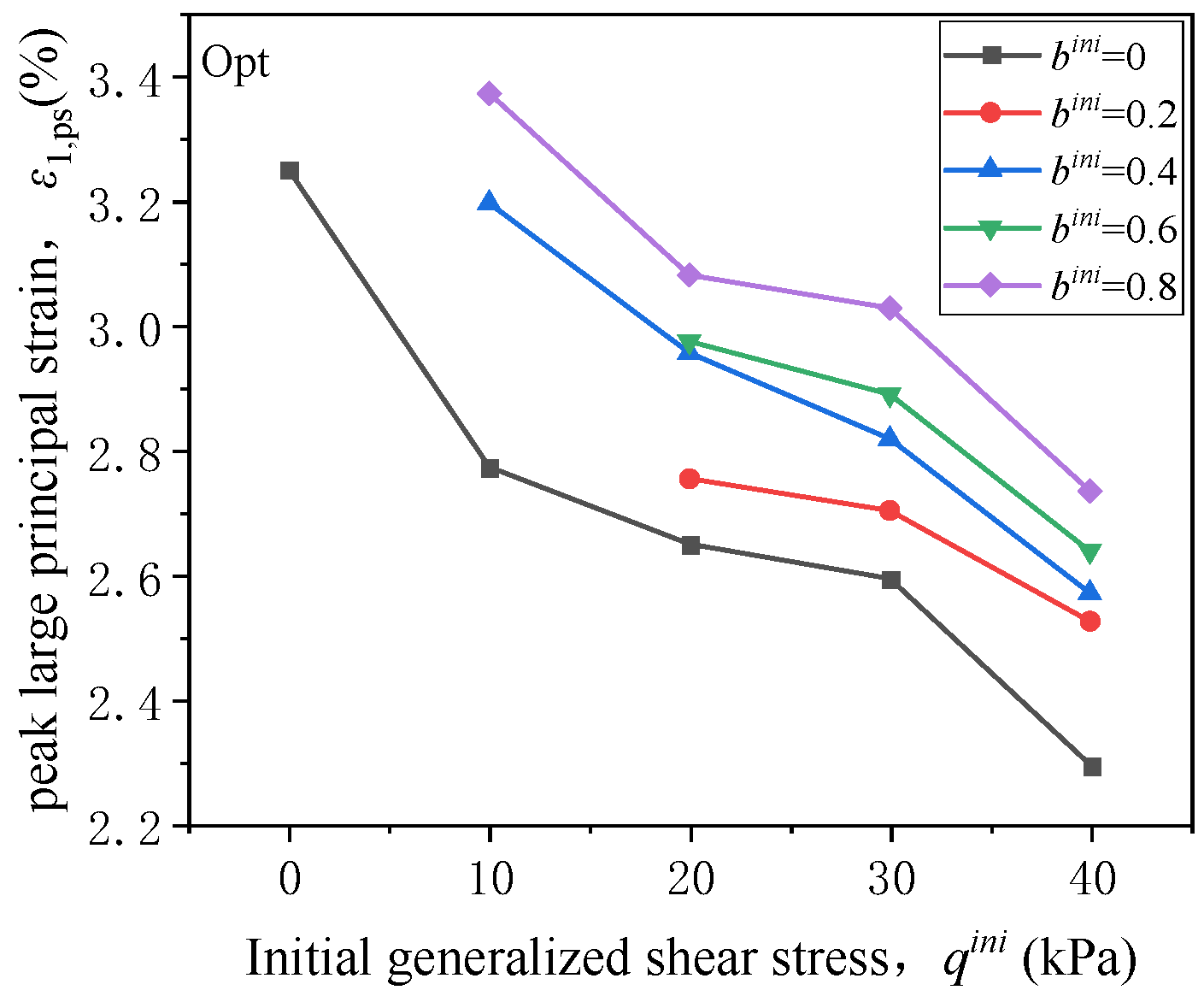
Figure 19 shows the relationship between the major principal strain at peak stress and qini. For different bini values, the major principal strain at peak stress generally decreases as qini increases, but the trend varies slightly across different ranges. When qini increases from 0 to 20 kPa, the major principal strain decreases rapidly. In the range of 20–30 kPa, the decline slows, but beyond 30 kPa, it decreases rapidly again. These results indicate that under the same initial mean principal stress, the effect of qini on soil deformation is minimal within the range of 20–30 kPa.
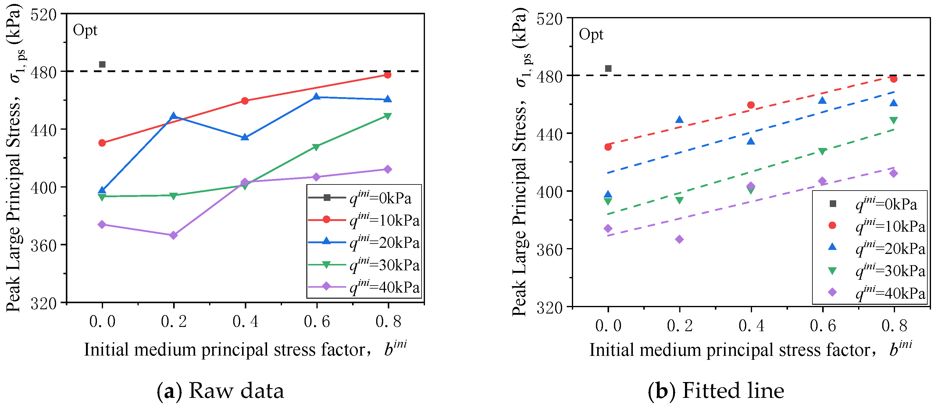
To analyze the effect of the initial intermediate principal stress coefficient bini on the peak major principal stress, Figure 20a shows the relationship between the peak major principal stress of coarse-grained soil at optimum water content and bini under different initial generalized shear stresses qini. Overall, the peak major principal stress is positively correlated with bini; as bini increases, the peak major principal stress also increases.
When bini increases from 0 to 0.8, the peak major principal stresses for qini = 10, 20, 30, and 40 kPa increase by 11%, 16%, 14%, and 10%, respectively, with relatively small differences. This indicates that the influence of bini on the peak major principal stress is independent of qini. Furthermore, considering experimental errors, the relationship between the peak major principal stress and bini can be approximately regarded as linear.
Based on Figure 20a, Figure 20b uses a linear equation (Equation (13)) to fit the relationship between the peak major principal stress and bini. The specific fitting parameters are provided in Table 5.
σ 1 , ps = e + f b i n i
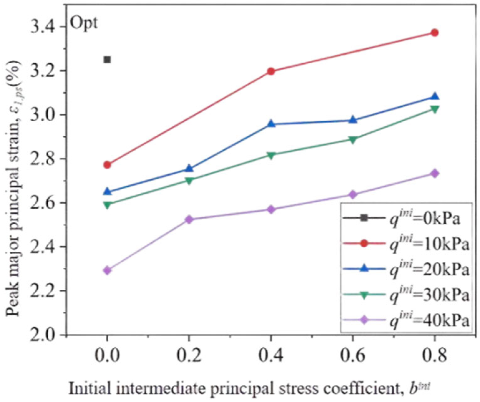
Figure 21 presents the relationship curve between the major principal strain at peak stress and the initial intermediate principal stress coefficient (bini). Similar to Figure 20, under different initial generalized shear stresses (qini), the major principal strain at peak stress increases approximately linearly with the increase in bini. Table 5 lists the initial generalized shear stress (qini) for the different fitting parameters used in this study.
Taking qini = 30 kPa as an example, when bini changes from 0 to 0.8, the corresponding major principal strains at peak stress are 2.59%, 2.70%, 2.82%, 2.89%, and 3.03%, with differences of 0.11%, 0.12%, 0.07%, and 0.14%, respectively.

3.2.2. Comparison Between Saturated and Optimum Water Content Conditions

Figure 22a,b compares the relationships of peak major principal stress with the initial generalized shear stress (qini) and initial intermediate principal stress coefficient (bini) under saturated and optimum water content conditions. The test results under the initial isotropic state (qini = 0, bini = 0) are included in Figure 22a. Similar to the optimum water content specimens, the increase in qini leads to a significant reduction in the peak major principal stress of saturated specimens. Figure 22b shows that the peak major principal stress of saturated specimens also increases with bini, and the trends of the two curves are very similar, indicating that the effect of bini on the peak major principal stress is not significantly influenced by the soil’s water content. Additionally, Figure 22 reveals that in all cases, the peak major principal stress of saturated specimens is lower than that of optimum water content specimens, with an average difference of approximately 40 kPa, accounting for about 10% of the peak strength of saturated specimens (ranging from 8% to 12.4%). This suggests that the lubricating effect of water makes it easier for the soil particles to slide over each other, leading to a higher likelihood of failure.
Figure 23a,b shows the relationships of peak major principal strain with initial generalized shear stress (qini) and initial intermediate principal stress coefficient (bini) under saturated and optimum water content conditions. Similar to Figure 22, the test results under saturated and optimum water content conditions are comparable. The peak major principal strain gradually decreases with an increase in qini and increases with an increase in bini. However, the peak major principal strain of saturated coarse-grained soil is consistently smaller than that of coarse-grained soil at optimum water content.

3.2.3. Stress Ratio

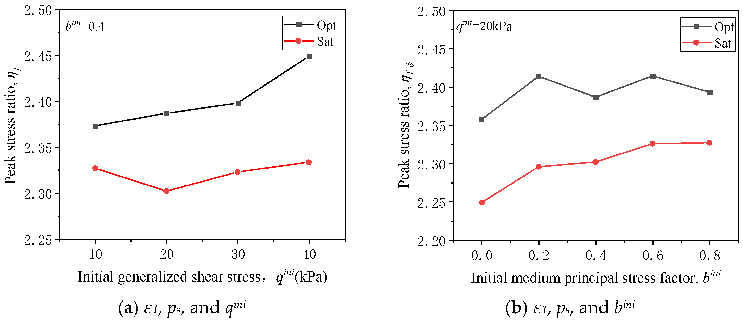
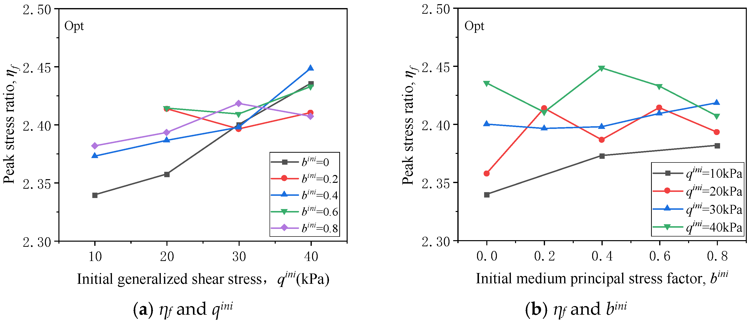
Figure 24a,b shows the relationships between the peak stress ratio and the initial generalized shear stress (qini) as well as the initial intermediate principal stress coefficient (bini) under optimum water content conditions. Overall, the peak stress ratio of coarse-grained soil increases rapidly with an increase in qini, while its variation with bini is not significant, showing a slight upward trend except for qini = 40 kPa.
It is worth noting that although the peak major principal stress decreases with an increase in qini in Figure 18a, the peak stress ratio in Figure 24a does not decrease accordingly, but instead shows an increasing trend. This is similar to the phenomenon observed in isotropic shear tests, where the peak stress increases with the confining pressure while the peak stress ratio decreases. This behavior can also be explained based on the stress path.
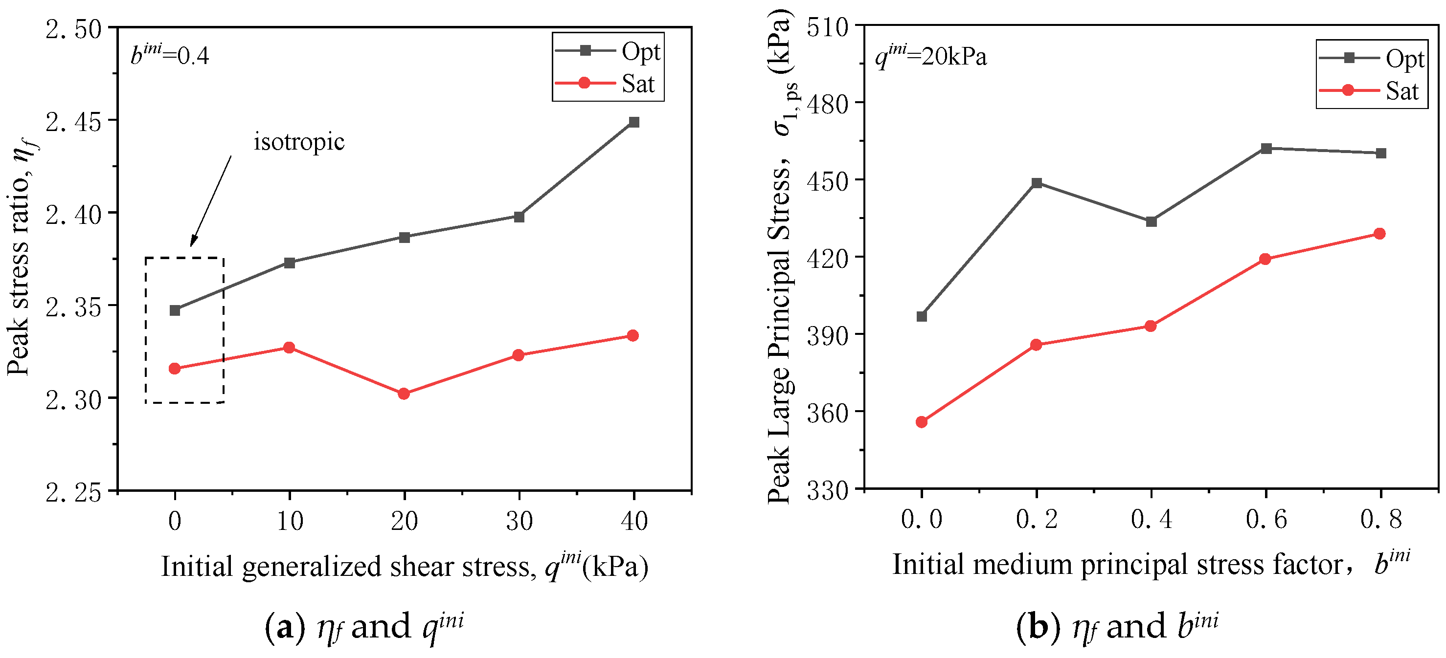
To analyze the effect of water content on the peak stress ratio, Figure 25 compares the relationships between the peak stress ratio and the initial generalized shear stress (qini) as well as the initial intermediate principal stress coefficient (bini) under saturated and optimum water content conditions. In Figure 25a, the test results under the initial isotropic state (qini = 0, bini = 0) are included.
As shown in Figure 25, the peak stress ratio of saturated specimens is lower compared to that of specimens with optimum water content. However, the development trends of the peak stress ratio with qini and bini for the saturated specimens are generally consistent with those of optimum water content specimens. Combined with Figure 24, this further confirms the conclusion that the peak stress ratio increases with an increase in qini and bini.

3.2.4. Modulus

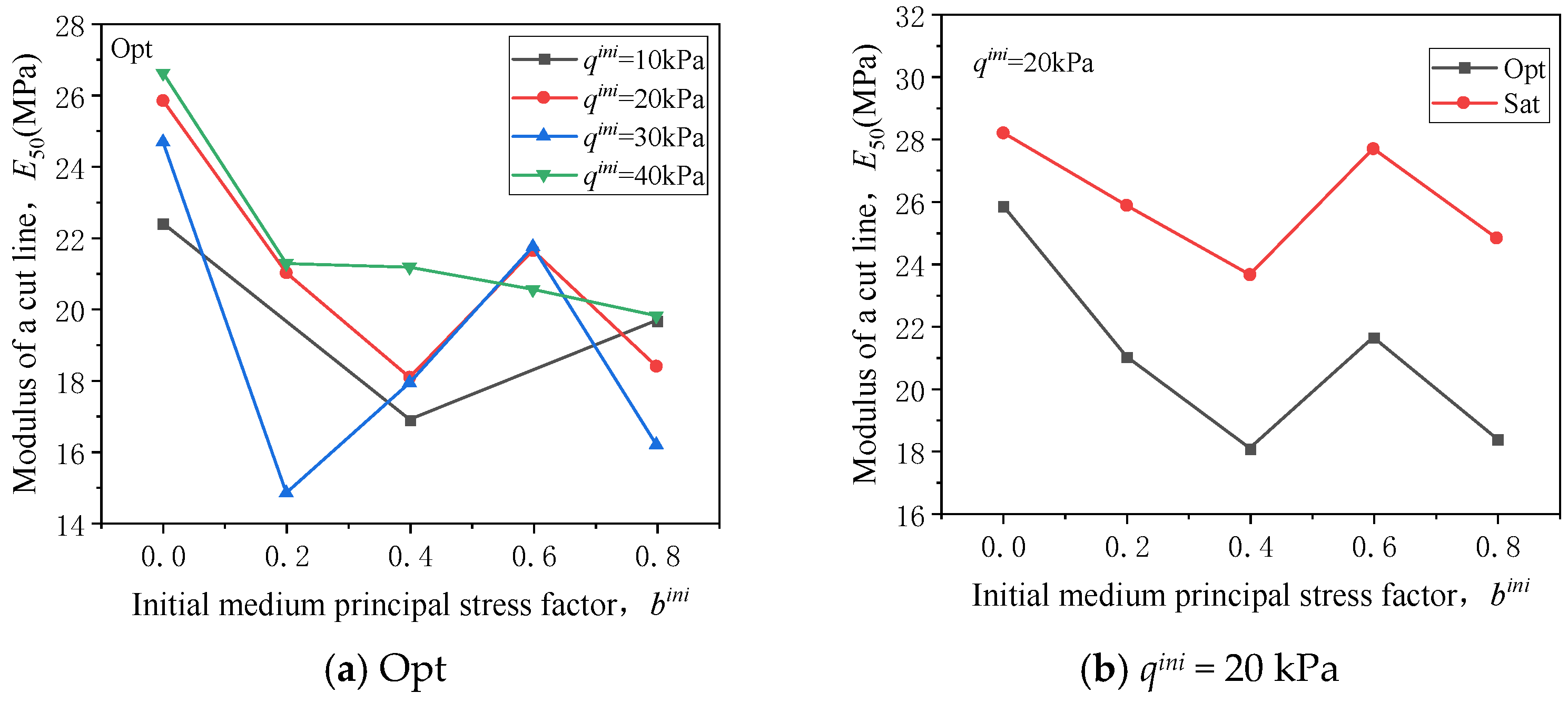
Figure 26a shows the relationship between the secant modulus (E50) and the initial intermediate principal stress coefficient (bini) under optimum water content conditions. It can be observed that under different initial generalized shear stresses (qini), the secant modulus is generally at a higher level when bini = 0, and then decreases to some extent as bini increases. However, this decrease is not entirely monotonic. Section 2 discussed the relationship between the direction of generalized shear stress and bini, with bini indirectly representing the direction of the generalized shear stress. This indicates that under different initial generalized shear stresses, the stiffness of coarse-grained soil is influenced by the direction of generalized shear stress, and the stiffness is maximized when bini = 0 (θ = −30°).
Figure 26b presents the relationship between the secant modulus and bini under both saturated and optimum water content conditions. The trends of the two curves are consistent, and the secant modulus under saturated conditions is greater than that under optimum water content conditions. This is similar to the results of isotropic shear tests (Figure 9b).

3.3. Test Results and Analysis of Static Shear Characteristics of Coarse-Grained Soil Under Plane Strain Conditions

3.3.1. Stress–Strain Relationship and Strength

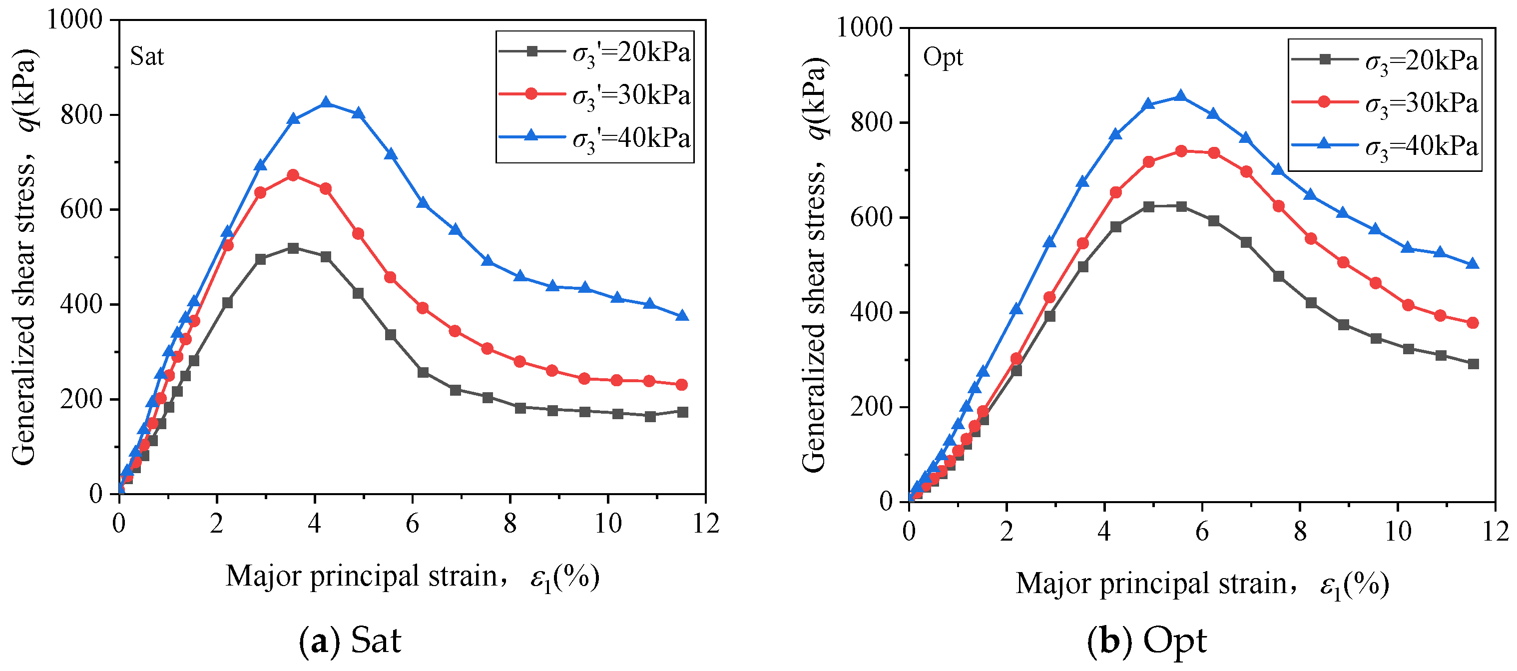
Figure 27 shows the relationship curves between the generalized shear stress and major principal strain under plane strain conditions for coarse-grained soil. It can be observed that under different confining pressures, the soil exhibits significant strain-softening behavior. The generalized shear stress increases with the major principal strain at the initial stage of loading, reaches a peak, and then decreases rapidly. Under saturated conditions, the generalized shear stress stabilizes and approaches the critical state when the major principal strain reaches approximately 12%.
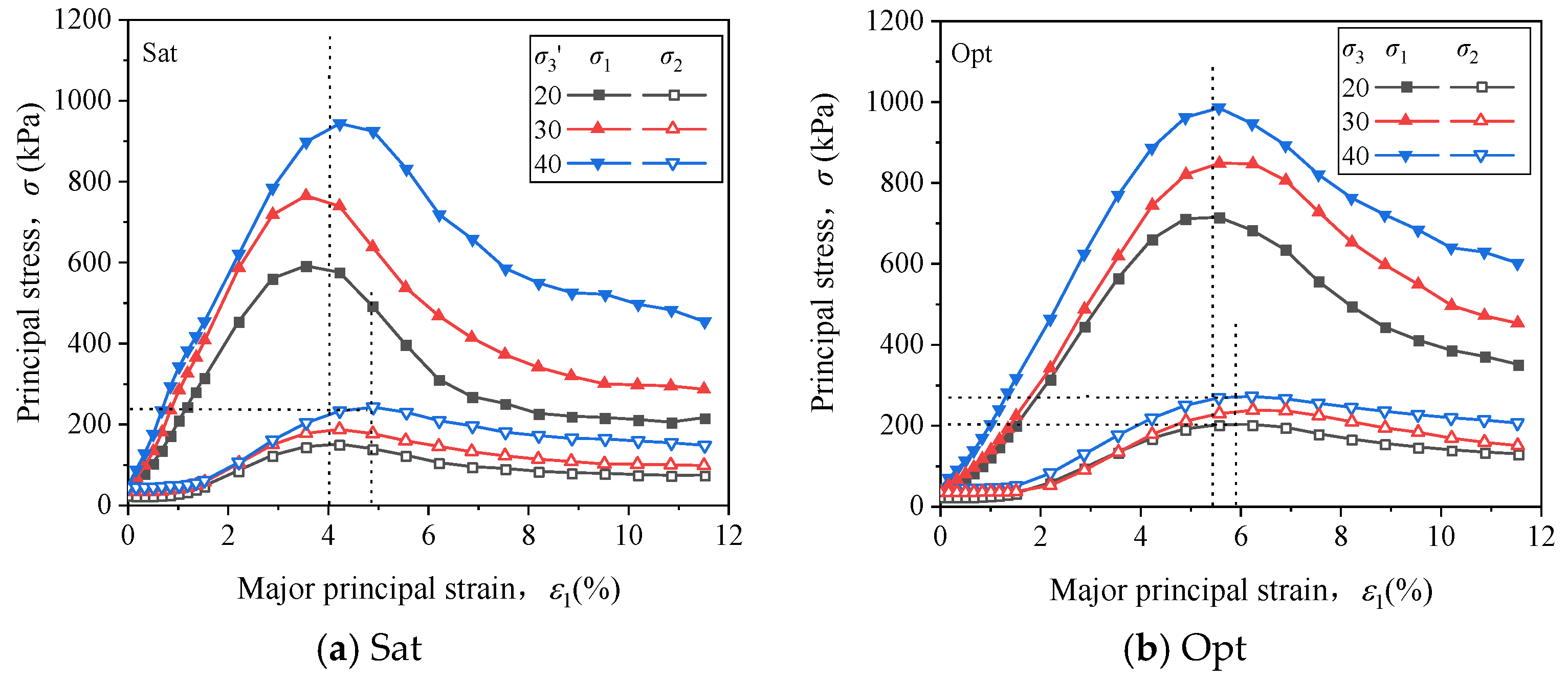
Figure 28 presents the relationship curves of major principal stress (σ1), intermediate principal stress (σ2), and major principal strain. Combined with Figure 27 and Figure 28, it can be seen that the development trend of the major principal stress is entirely consistent with that of the generalized shear stress, differing only in magnitude. Compared to the optimum water content condition, both the peak generalized shear stress (or peak major principal stress) and the peak major principal strain are lower under saturated conditions. Specifically, the peak major principal strain under saturated conditions ranges from 3% to 5%, while under optimum water content conditions, it ranges from 4% to 6%. Additionally, Figure 28 shows that the development of the intermediate principal stress exhibits a certain lag. The peak of the intermediate principal stress (σ2) always occurs later than the peak of the major principal stress (σ1). The statistical calculations indicate that the intermediate principal stress reaches its peak, approximately 0.5% major principal strain, after the peak of the major principal stress.
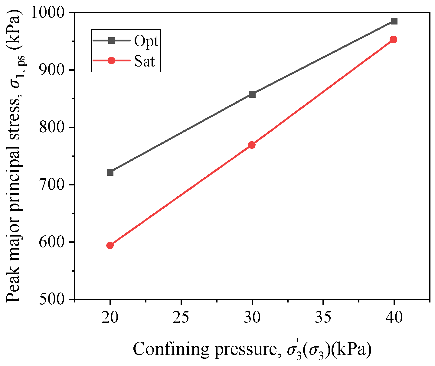
By comparing Figure 28 and Figure 6, it can be seen that, similar to the results of isotropic shear tests, the peak major principal stress increases with an increase in the confining pressure. To further analyze the relationship between the major principal stress and confining pressure, Figure 29 illustrates the relationship curves of peak major principal stress versus confining pressure under different water content conditions.
The results show a strong linear relationship between the peak major principal stress and the confining pressure. Additionally, as the confining pressure increases, the difference in the peak major principal stress between the saturated and optimum water content conditions decreases. This indicates that the influence of water content on the peak strength of the soil diminishes with an increasing confining pressure.

3.3.2. Modulus

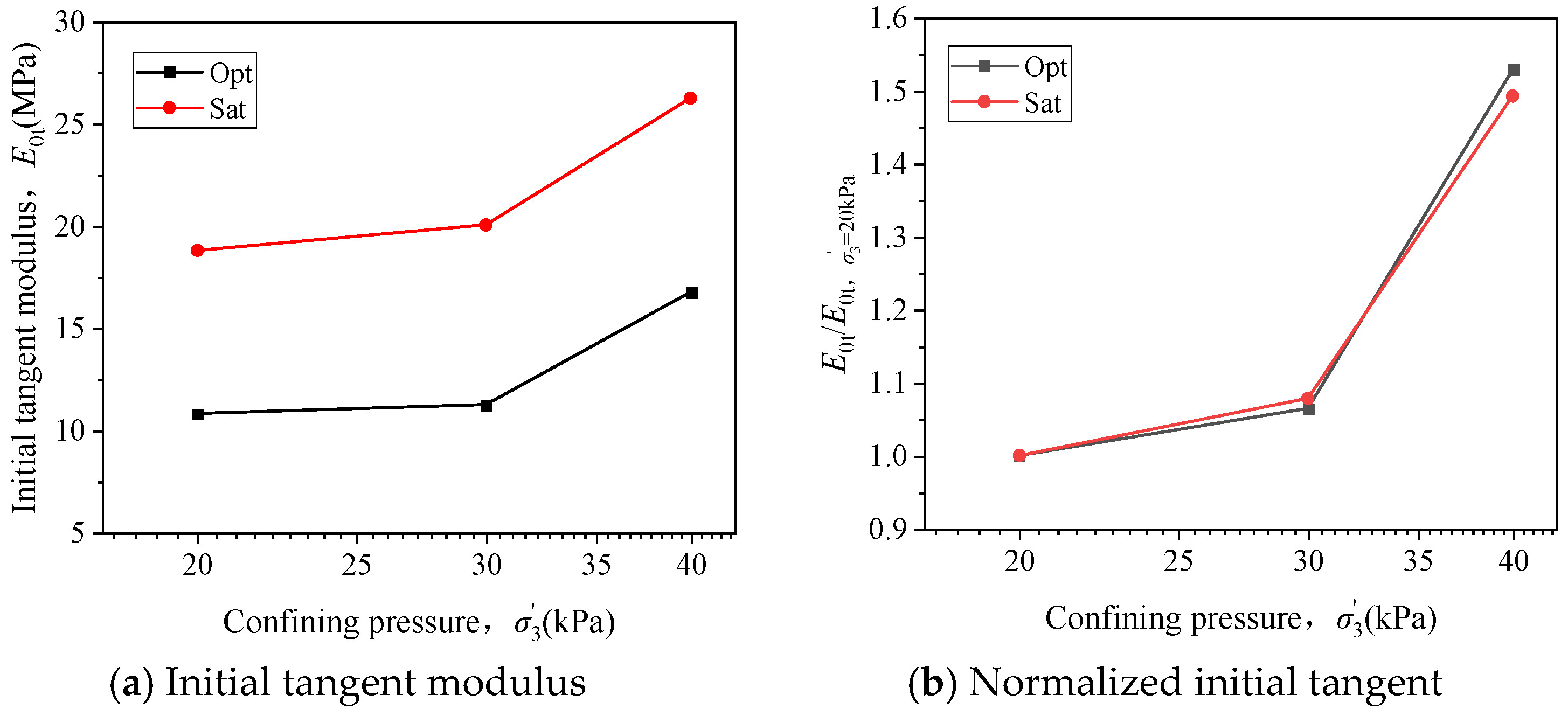
Figure 30a shows the relationship between the initial tangent modulus (E0t) and the confining pressure ( σ 3 ) under plane strain conditions. It can be observed that the initial tangent modulus (E0t) increases with an increase in the confining pressure. Under different confining pressures, the initial tangent modulus under saturated conditions (E0t-Sat) is consistently greater than that under optimum water content conditions (E0t-Opt). The differences between the two conditions for confining pressures of 20 kPa, 30 kPa, and 40 kPa are 5.51 MPa, 6.44 MPa, and 8.14 MPa, respectively.
To further analyze the effect of confining pressure on the initial tangent modulus (E0t), Figure 30b provides the normalized curves of the initial tangent modulus relative to the confining pressure. It can be seen that, under plane strain conditions, unlike the isotropic stress state, the initial tangent modulus (E0t) and lg σ 3 do not exhibit a linear relationship. Moreover, the normalized curves under both water content conditions almost overlap, indicating that under plane strain conditions, the water content has little effect on the relationship between the initial tangent modulus and the confining pressure.
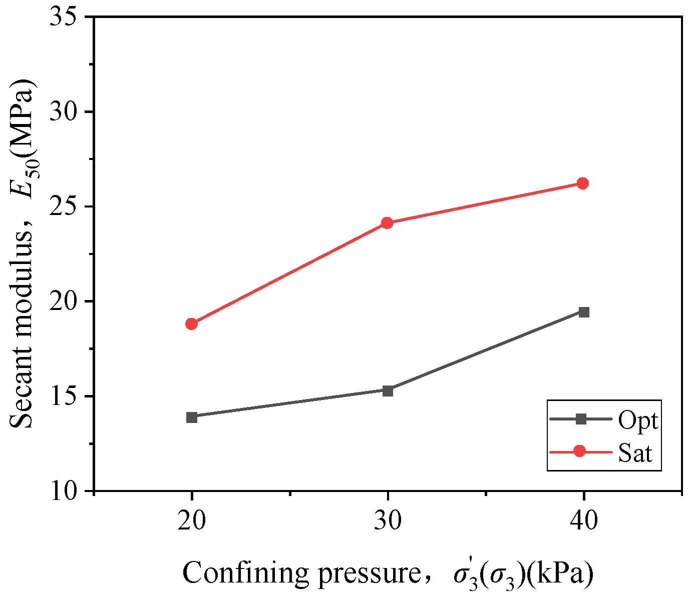
Figure 31 illustrates the relationship between the secant modulus (E50) and confining pressure ( σ 3 ) under plane strain conditions. It can be observed that the secant modulus increases with an increase in the confining pressure. Similar to the initial tangent modulus, the secant modulus under saturated conditions is greater than that under optimum water content conditions, consistent with the conclusions drawn from the isotropic shear tests.

3.3.3. Intermediate Principal Stress and Intermediate Principal Stress Coefficient (b)

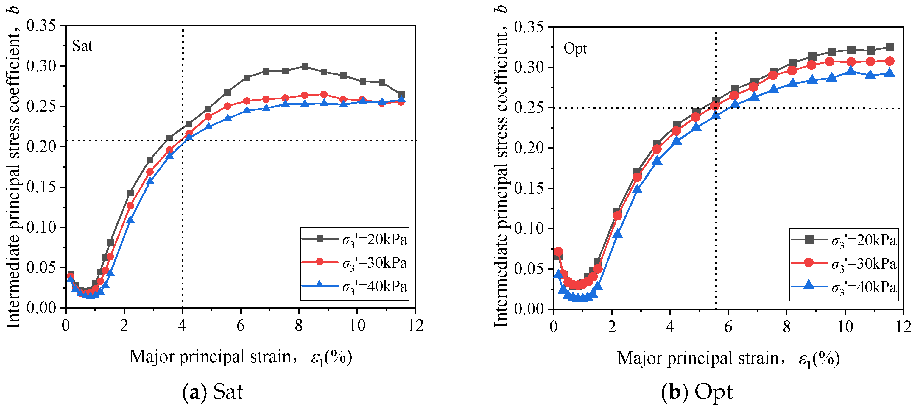
Figure 32 shows the relationship curves between the intermediate principal stress coefficient (b) and the major principal strain under plane strain conditions. The vertical dashed lines in the figure represent the points of peak strength. First, it can be observed that under both saturated and optimum water content conditions, there are slight initial b-values at the beginning of the tests. This is caused by the axial force applied to the specimen during the test, leading to minor errors, which can be ignored. As the test progresses, starting from approximately 1% major principal strain, the intermediate principal stress coefficient (b) increases rapidly with an increase in the major principal strain. After reaching the peak strength, the development trend of b begins to slow and eventually stabilizes.
Additionally, Figure 32 shows that the b-value corresponding to the peak strength under optimum water content conditions is approximately 0.25, while under saturated conditions it is around 0.20. The research has indicated that for unsaturated coarse-grained soil specimens under high confining pressures (100 kPa ≤ σ 3 ≤ 400 kPa), the b-value at failure ranges between 0.15 and 0.20, and there is a phenomenon where the intermediate principal stress coefficient (b) decreases with increasing confining pressure. Furthermore, a study reported that for plane strain tests on Lianghekou mixed material and slate material, the b-value at peak strength never exceeds 0.25. At the same confining pressure, the results of plane strain tests fall between those of true triaxial tests, with b = 0 and b = 0.25 under constant σ3 and constant b conditions.
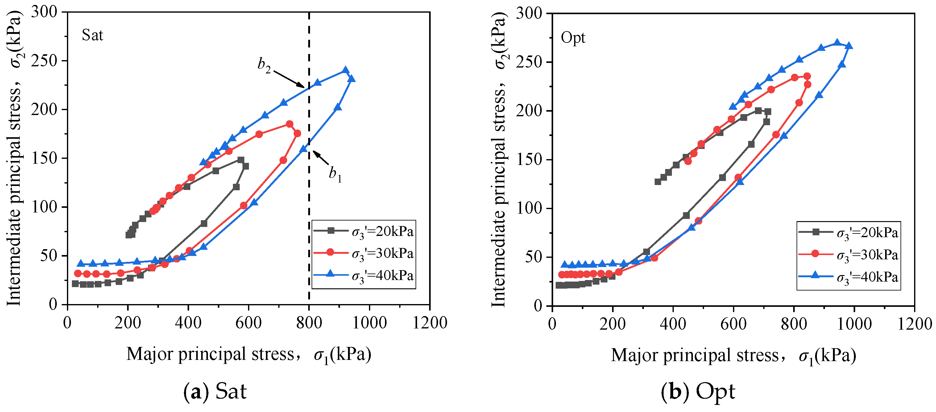
To clarify why the maximum intermediate principal stress coefficient (b) does not occur at the point of peak strength, Figure 33 presents the relationship curves between the intermediate principal stress (σ2) and the major principal stress (σ1). It can be observed that the curve is divided into loading and unloading stages. After the stress reaches the peak and unloading begins, the unloading curve lies above the loading curve. For the same major principal stress, the intermediate principal stress during unloading is larger than that during loading. According to the formula for calculating the intermediate principal stress coefficient (b), and given that the confining pressure ( σ 3 ) remains constant during the test, the b-value during the unloading stage is greater than that during the loading stage, i.e., b1 < b2.

3.4. Comparison of Shear Characteristics Between Initial Isotropic Stress State and Plane Strain State

3.4.1. Strength and Modulus

Figure 34 compares the generalized shear stress–major principal strain relationship curves for coarse-grained soil under initial isotropic stress conditions and plane strain conditions. First, it can be observed that under the same confining pressure, the peak generalized shear stress (qps, p) and residual generalized shear stress (qr, p) under plane strain conditions are both greater than their corresponding values under initial isotropic stress conditions. This indicates that the constraint effect of the intermediate principal stress significantly enhances the soil’s shear strength. For example, under optimum water content conditions with a confining pressure of σ3 = 40 kPa, the peak generalized shear stresses under plane strain and isotropic stress conditions are 854.5 kPa and 444.4 kPa, respectively, with the former being 1.93 times the latter. Additionally, it can be observed that within the range of 2% major principal strain, the plane strain curve lies below the isotropic stress curve. This suggests that the initial tangent modulus under plane strain conditions is smaller than that under isotropic stress conditions.
To analyze the modulus relationship under the two stress states, Figure 35a,b shows the relationships of initial tangent modulus and secant modulus with the confining pressure for plane strain and isotropic stress conditions. Both moduli increase with the confining pressure, but the rate of increase differs. For example, under optimum water content, when the confining pressure increases from 20 kPa to 40 kPa, the initial tangent modulus under plane strain conditions increases from 9.20 MPa to 13.75 MPa, while under isotropic stress conditions it increases from 11.0 MPa to 20.5 MPa, showing a much higher growth rate. At the same confining pressure and water content, the initial tangent modulus under plane strain conditions is consistently smaller than under isotropic stress conditions. The same trend is observed for the secant modulus, which is also smaller under plane strain conditions.

3.4.2. Volumetric Strain

Figure 36 illustrates the generalized shear stress volumetric strain relationship curves for coarse-grained soil under initial isotropic stress and plane strain conditions, where volumetric compression is defined as positive and dilation as negative. From the start of loading, all the specimens exhibit compression, with the volume decreasing until the maximum compression is reached. At this point, the trend reverses, and the volumetric strain transitions through zero, marking the onset of dilation.
Careful observation shows that before reaching the maximum compression, the generalized shear stress curves under plane strain and isotropic stress conditions are nearly identical across all confining pressures. This indicates that during the initial compression stage, plane strain tests can closely approximate conventional triaxial tests. However, once the volumetric strain exceeds zero, the constraint in the intermediate principal stress direction under plane strain conditions causes the stress values to be significantly higher than those under isotropic stress conditions for the same volumetric strain.

3.4.3. Friction Angle

Figure 37 compares the relationship curves of peak friction angle and confining pressure under two initial stress states. It is evident that at low confining pressures, the peak friction angle (φps) under plane strain conditions is significantly greater than that under isotropic stress conditions. Additionally, the peak friction angle shows a good linear relationship with the logarithm of confining pressure (lg σ 3 ), decreasing as the confining pressure increases. This trend is consistent with findings from other studies on fine-grained and coarse-grained soils.
Table 6 summarizes the peak friction angles from the isotropic and plane strain tests, as well as the percentage differences between them. The table shows that under different water content conditions, the percentage difference in the peak friction angle between plane strain and isotropic stress states gradually increases with the confining pressure. Although the difference is small, it indicates to some extent that the gap in the peak friction angles between the two stress states widens as the confining pressure increases. Additionally, it can be observed that the peak friction angles of saturated specimens are consistently smaller than those of specimens at optimum water content.

3.4.4. Stress Ratio

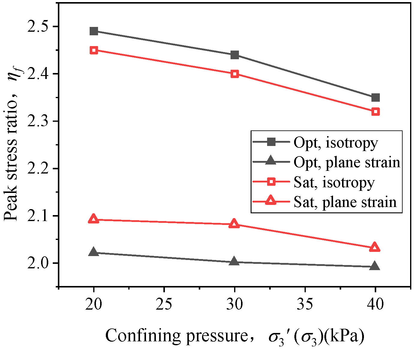
Figure 38 shows the relationship curves of peak stress ratio ( η f ) and confining pressure under two initial stress states. It can be seen that the peak stress ratio decreases with an increasing confining pressure. The peak stress ratio under plane strain conditions is significantly lower than that under isotropic stress conditions.
Under saturated conditions, the difference between the two is relatively small, with the peak stress ratio decreasing by 12.5% to 14.7%. Under optimum water content conditions, the peak stress ratio decreases by 15.3% to 18.9%. The relevant research indicates that under high confining pressures (100 kPa ≤ σ 3 ≤ 400 kPa), the peak stress ratio of unsaturated specimens under plane strain conditions is 13% to 18% lower than that under conventional triaxial compression conditions. Similar to the findings in this study, the difference between the two decreases as the confining pressure increases.

3.5. Comparison of Volumetric Strain Under Different Initial Stress States and the Dilatancy Equation

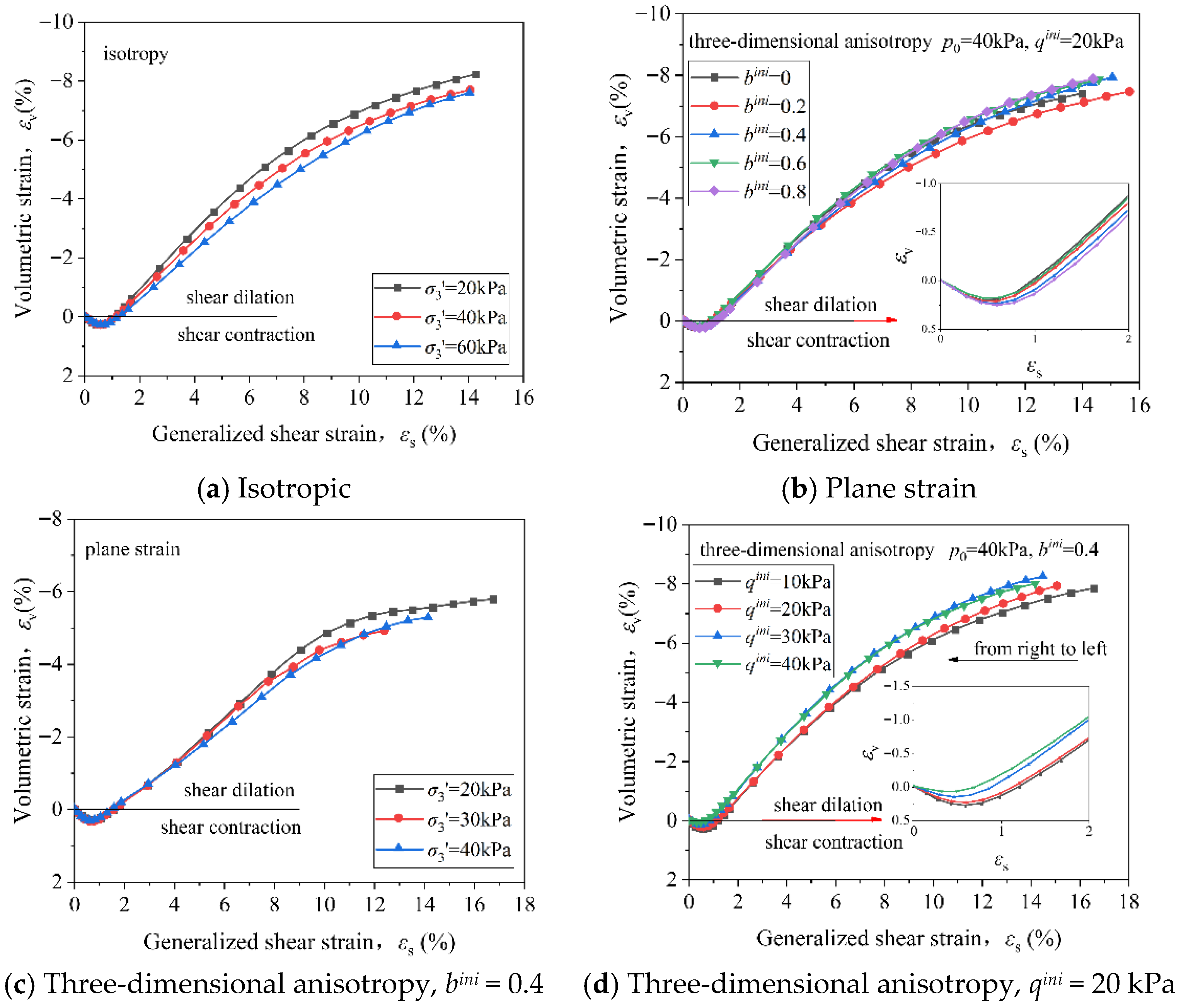
Figure 39 shows the relationship curves between the volumetric strain and generalized shear strain under three different initial stress states. All the specimens exhibit the phenomenon of initial compression followed by dilation as the generalized shear strain increases, indicating that as the generalized shear stress grows, the particle motion transitions from filling voids to the rotation and rearrangement of adjacent particles. In Figure 38a,b, which displays the volumetric strain–generalized shear strain relationship under isotropic and plane strain conditions at different confining pressures, it can be observed that the volumetric strain decreases with increasing confining pressure. Under isotropic stress conditions, when the confining pressure is 60 kPa, the specimen shows the smallest maximum compression. Under plane strain conditions, the volumetric strain curves at the initial stage (0< εs <4%) are almost completely identical.
Figure 38c,d depicts the effects of initial generalized shear stress and the initial intermediate principal stress coefficient (b) on the volumetric strain under three-dimensional initial anisotropic stress states. Except for a few tests where b = 0.6, within the range of 2% generalized shear strain, the volumetric strain increases with the initial generalized shear stress, while it decreases with an increase in the initial intermediate principal stress coefficient (b).
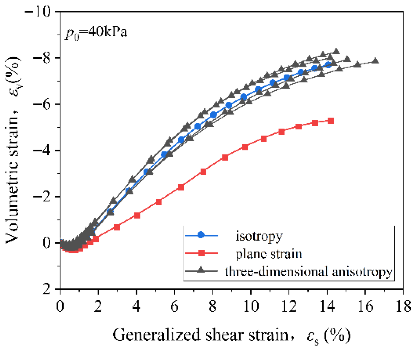
Figure 40 presents the relationship curves between the volumetric strain and generalized shear strain under three initial stress states, with an initial mean principal stress of 40 kPa. It can be observed that, under the same initial mean stress, the volumetric strain curve for the isotropic condition is entirely enclosed by the volumetric strain curves of the three-dimensional initial anisotropic stress condition. In contrast, the volumetric strain curve for the plane strain condition lies far below the aforementioned curves. This indicates that under plane strain conditions, the volumetric deformation of coarse-grained soil is significantly suppressed, resulting in much higher soil strength compared to the isotropic and three-dimensional initial anisotropic stress conditions.
From the above volumetric strain curves, it can be seen that coarse-grained soil exhibits strong dilatancy under a low confining pressure. The degree of dilatancy for soil is usually measured by the dilatancy rate d, which is generally expressed as follows in Equation (14):
d = d ε v p d ε s p
where ε v p represents the plastic volumetric strain and ε s p represents the plastic generalized shear strain.
In the past, extensive research has been conducted on the dilatancy characteristics and dilatancy equations of coarse-grained soils. Among these, the modified Cambridge model dilatancy equation (Equation (15)) has been one of the most influential and widely applied. Burland et al. proposed a modified dilatancy equation based on the Cambridge model, as shown in Equation (16). However, under low confining pressures, the modified Cambridge model tends to overestimate the initial compression behavior of coarse-grained soils during the early stages of loading and underestimate the dilatancy behavior during the middle and later stages of loading. As a result, it fails to accurately represent the deformation characteristics of coarse-grained soils.
d = M η
d = M 2 η 2 2 η
Among the methods for improving the Cambridge model dilatancy equation, the most common approach is to replace the critical state stress ratio M with the dilatancy stress ratio Md, where Md is the stress ratio at the point when the soil transitions from contraction to dilation (the dilative state). Based on this improvement, Lagioia proposed a new dilatancy equation (Equation (17)). This equation allows for a better fit to the relationship between the dilatancy rate d and the stress ratio η by adjusting the material parameters μ and α. However, the ranges of μ and α are too large and difficult to determine, and the equation fails to accurately capture the dilatancy behavior of coarse-grained soils under low confining pressures.
d = μ ( M d η ) ( α M d η + 1 )
Based on this, a new dilatancy rate equation was developed, as shown in Equation (18). This equation effectively captures the behavior of coarse-grained soils in conventional triaxial shear tests under low confining pressures, reflecting the relatively weak contraction during the early loading stage and the stronger dilatancy during the middle and late loading stages. Moreover, the equation involves only one parameter, μ, making it simpler and more practical to use.
d = μ ( M d η ) ( M d η 2 + 1 ) ( M d 2 η + 1 )
where M represents the critical state stress ratio, η is the stress ratio during the test, M d denotes the dilatancy stress ratio (the stress ratio at the transition from contraction to dilation), and μ is the material-related parameter.
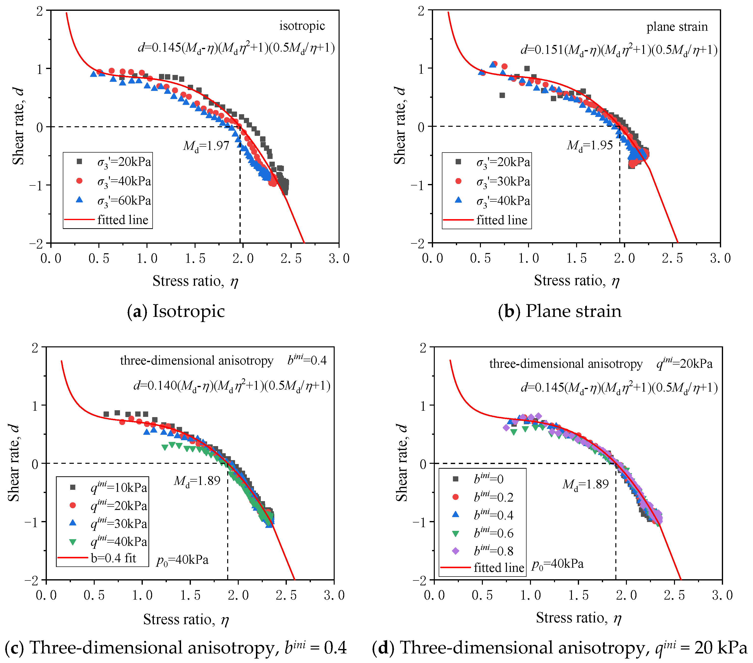
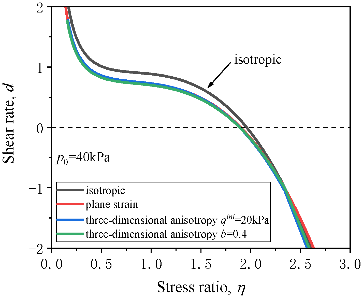
Figure 41 presents the fitted curves of the coarse-grained soil test results using Equation (18). It can be observed that this equation achieves a good fitting performance under different initial stress states. Furthermore, considering that all the coarse-grained soil specimens in this study have the same gradation, the values of the parameter μ under the different initial stress states are 0.145, 0.151, 0.140, and 0.145, respectively, showing very limited variation. This indicates that the initial stress state has a minimal effect on μ. To further analyze the influence of initial stress states on the dilatancy behavior of coarse-grained soils, Figure 42 summarizes the fitted curves under the different initial stress states. It can be seen that, compared to the plane strain and three-dimensional anisotropic stress states, the isotropic stress state slightly overestimates the contraction of coarse-grained soils but shows almost no difference in predicting their dilatancy behavior.
Additionally, from Figure 41c, it can be observed that under the three-dimensional initial anisotropic stress states, when η < Md, the dilatancy rate varies significantly for different qini. However, as η increases, the differences gradually diminish, and when ηMd, the dilatancy rates become nearly identical. This indicates that the initial generalized shear stress only has a certain impact on the contraction behavior of coarse-grained soils. Moreover, as shown in Figure 41d, the dilatancy rates under different bini values are extremely close to each other, indicating that the initial intermediate principal stress coefficient has no impact on the dilatancy behavior of coarse-grained soils.

4. Discussion

We acknowledge several valid drawbacks regarding the representativeness of coarse-grained soil testing, limitations of static loading protocols, statistical robustness of empirical correlations, and the fidelity of true triaxial simulations relative to field conditions.
In response, we have expanded datasets; clarified the material-specific limitations; incorporated discussions on dynamic effects and data normalization; and acknowledged experimental constraints, such as particle size scaling [9,10], moisture control [11,12], membrane friction, and incomplete replication of complex 3D stress paths [13,14].
While the current study provides controlled laboratory insights under defined stress states, we emphasize its role as a foundation for future work integrating cyclic/dynamic loading, advanced data processing, and micro-mechanical characterization to bridge the gap between lab results and field behavior.

5. Conclusions

Based on a GDS dynamic–static true triaxial apparatus, this study systematically investigates the effects of initial stress state parameters—such as the initial mean principal stress (initial confining pressure), initial generalized shear stress qini, and initial intermediate principal stress coefficient bini—as well as the water content on the static shear behavior of coarse-grained soils under three initial stress conditions: three-dimensional initial isotropic, three-dimensional initial anisotropic, and plane strain. The main conclusions are as follows:
(1) Under a three-dimensional initial isotropic stress state, there is a clear linear relationship between the confining pressure and peak major principal stress, initial tangent modulus E0t, peak friction angle φps, and peak stress ratio η f . Specifically, the peak major principal stress and initial tangent modulus increase with an increasing confining pressure, while the peak stress ratio and peak friction angle decrease as the confining pressure increases. Under saturated undrained conditions, the peak strength is significantly greater than under saturated drained conditions, while the initial tangent modulus is smaller. Moreover, the effect of confining pressure on the peak friction angle is more pronounced under undrained conditions.
(2) For a three-dimensional initial anisotropic stress state, the peak strength of coarse-grained soil decreases with increasing qini, and an increase in bini weakens the effect of qini on the peak strength. Meanwhile, the peak strength increases with an increasing bini, and the relationships between qini, bini, and the peak strength are approximately linear, leading to the establishment of corresponding linear equations. It was also observed that when bini = 0, the secant modulus of the coarse-grained soil reaches its maximum. Under plane strain conditions, the peak strength increases linearly with increasing confining pressure, and a certain lag is observed between the intermediate principal stress and the major principal stress. The maximum value of the intermediate principal stress coefficient b does not occur at the peak strength. For soils under optimal water content conditions, the b-value corresponding to the peak strength is approximately 0.25, while under saturated conditions, it is around 0.20. Both the initial tangent modulus and secant modulus increase with increasing confining pressure.
(3) Under different initial stress states and drainage conditions, the peak strength of coarse-grained soil with optimal water content is greater than that of saturated soil. For isotropic and plane strain initial stress states, the peak friction angle of coarse-grained soil with optimal water content is slightly greater than that of saturated soil. For isotropic and anisotropic initial stress states, the peak stress ratio of coarse-grained soil with optimal water content is greater than that of saturated soil, whereas under plane strain conditions, the peak stress ratio of coarse-grained soil with optimal water content is smaller than that of saturated soil. When the initial mean principal stress is the same, the peak strength and peak friction angle of coarse-grained soil under plane strain conditions are greater than those under three-dimensional initial isotropic conditions. However, the peak stress ratio and initial tangent modulus under plane strain conditions are smaller than those under three-dimensional initial isotropic conditions. Furthermore, the peak strength of coarse-grained soil under three-dimensional initial isotropic stress is greater than that under three-dimensional initial anisotropic stress.
(4) Finally, the improved dilatancy rate equation was applied to fit the coarse-grained soil test results, and it was found that the equation performs well under different initial stress states, demonstrating its reliability and ability to capture the dilatancy behavior of coarse-grained soils.

Author Contributions

Conceptualization, Y.S. and W.Q.; Methodology, Y.C., W.Q. and Y.F.; Software, W.Q., Y.F., Z.H. and K.W.; Validation, Y.C., Y.F., Z.H. and K.W.; Formal analysis, Y.S., Y.C., W.Q., Y.F. and Z.H.; Investigation, Y.S., Y.C. and Z.H.; Resources, Y.S. and W.Q.; Data curation, Y.C., Y.F., Z.H. and K.W.; Writing—original draft, Y.S., Y.C., W.Q., Y.F., Z.H. and K.W.; Writing—review & editing, Y.S., Y.C., W.Q. and Y.F.; Visualization, Y.S., Y.C., Y.F., Z.H. and K.W.; Supervision, Y.S. and W.Q.; Project administration, Y.S., Y.C. and W.Q.; Funding acquisition, W.Q. All authors have read and agreed to the published version of the manuscript.

Funding

This research received no external funding.

Data Availability Statement

The original contributions presented in this study are included in the article. Further inquiries can be directed to the corresponding authors.

Conflicts of Interest

Author Yi Shi and Yongwei Chen was employed by the company Wenzhou Electrical Power Design Co., Ltd. The remaining authors declare that the research was conducted in the absence of any commercial or financial relationships that could be construed as a potential conflict of interest.

Abbreviations

The following abbreviations are used in this manuscript:
GDSGeo-technical Data System
CTComputed Tomography

References

  1. Li, X.J.; Zhu, M.X.; Dai, G.L.; Wang, L.Y.; Liu, J. Interface Mechanical Behavior of Flexible Piles Under Lateral Loads in OWT Systems. China Ocean Eng. 2023, 37, 484–494. [Google Scholar] [CrossRef] [Scilit]
  2. Qin, W.; Wu, H.; Ouyang, H.R.; Pan, Y.Q.; Ye, C.; Dong, X.D. Lateral cyclic load behavior of pile in coastal clay improved by vacuum preloading (VPM). Int. J. Phys. Model. Geotech. 2025, 25, 297–312. [Google Scholar]
  3. Cheng, X.L.; Liu, M.M.; Li, Q.; Lu, D.C.; Du, X.L. Dynamic response and fatigue damage analysis of offshore wind turbines supported by four-pile jacket in clays under typhoons. Acta Geotech. 2025, 20, 2461–2481. [Google Scholar] [CrossRef] [Scilit]
  4. Wang, B.X.; Wang, P.G.; Zhao, M.; Du, X.L. Three-Dimensional Fully Coupled Analytical Solution for a Water-Pile-Saturated Soil System Under Vertical P-wave Incident. Appl. Math. Model. 2025, 138, 115825. [Google Scholar] [CrossRef] [Scilit]
  5. Shi, Y.; Chen, Y.W.; Qin, W.; Zhou, Z.; Peng, G.; Lou, K.; Liu, Y. Study on Creep Behavior of Wenzhou Remolded Coastal Silt Under One-Dimensional and Triaxial Tests. Buildings 2025, 15, 3378. [Google Scholar] [CrossRef] [Scilit]
  6. Yang, F.; Wang, W.B.; Xie, Z.W.; Ma, Y.Y.; Lv, X.L. Experimental study on mechanical characteristics of coarse-grained materials of subgrade under static-dynamic loading. Chin. J. Geotech. Eng. 2023, 45, 247–252. [Google Scholar] [CrossRef]
  7. Zhou, Y.F.; Pan, J.J.; Cheng, Z.L.; Zuo, Y.Z. Behaviour of coarse-grained soil with rotation path of stress Lode’s angle. Chin. J. Geotech. Eng. 2020, 42, 55–59. [Google Scholar] [CrossRef]
  8. Cheng, X.L.; Wang, T.J.; Zhang, J.X.; Wang, P.; Tu, W.; Li, W. Dynamic response analysis of monopile offshore wind turbines to seismic and environmental loading considering the stiffness degradation of clay. Comput. Geotech. 2023, 155, 105210. [Google Scholar] [CrossRef] [Scilit]
  9. Liu, M.C.; Meng, F.; Wang, Y.Y. Evolution of particle crushing of coarse-grained materials in large-scale triaxial tests. Chin. J. Geotech. Eng. 2020, 42, 561–567. [Google Scholar] [CrossRef]
  10. Zhao, G.F.; Jiang, M.J.; Zhang, Z.; Wang, T.C.; Mei, G.X. Experimental study on permeability coefficient test method of coarse-grained soil with scaled gradation. Adv. Eng. Sci. 2024, 56, 240–246. [Google Scholar] [CrossRef]
  11. Mao, H.Y.; Liu, S.H.; Shen, C.M.; Wang, T.; Wang, L.J. Triaxial shear mechanical properties of weak rock coarse granular materials subjected to temperature and relative humidity. Chin. J. Geotech. Eng. 2024, 46, 587–595. [Google Scholar] [CrossRef]
  12. Guo, W.L.; Cai, Z.Y.; Zhu, J.G. Three state variables-related constitutive model for coarse-grained soil. Chin. J. Geotech. Eng. 2025, 47, 234–242. [Google Scholar] [CrossRef]
  13. Wu, E.L.; Zhu, J.G.; Huang, W.; Liu, Z. Evolution law of particle breakage of coarse-grained soil during triaxial shearing. Chin. J. Geotech. Eng. 2020, 42, 2330–2335. [Google Scholar] [CrossRef]
  14. Xu, W.W.; Xie, Z.D.; Fu, Z.Z.; Mi, Z.K. Research and application on true triaxial test of coarse-grained soil using Shen’s elastoplastic model. Rock Soil Mech. 2025, 46, 2559–2572. [Google Scholar]
Figure 1. GDS true triaxial apparatus.
Buildings 16 00233 g001
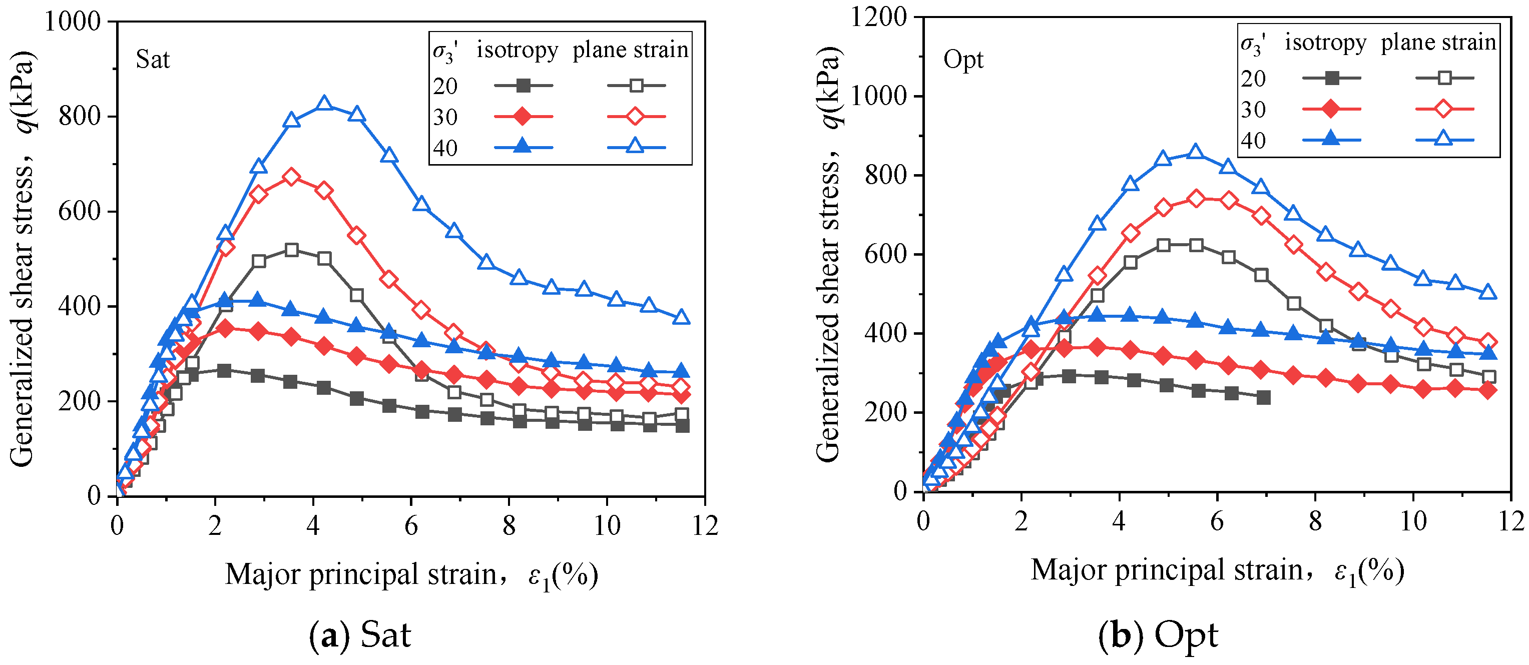
Figure 2. GDS dynamic and static true triaxial system structure diagram.
Buildings 16 00233 g002
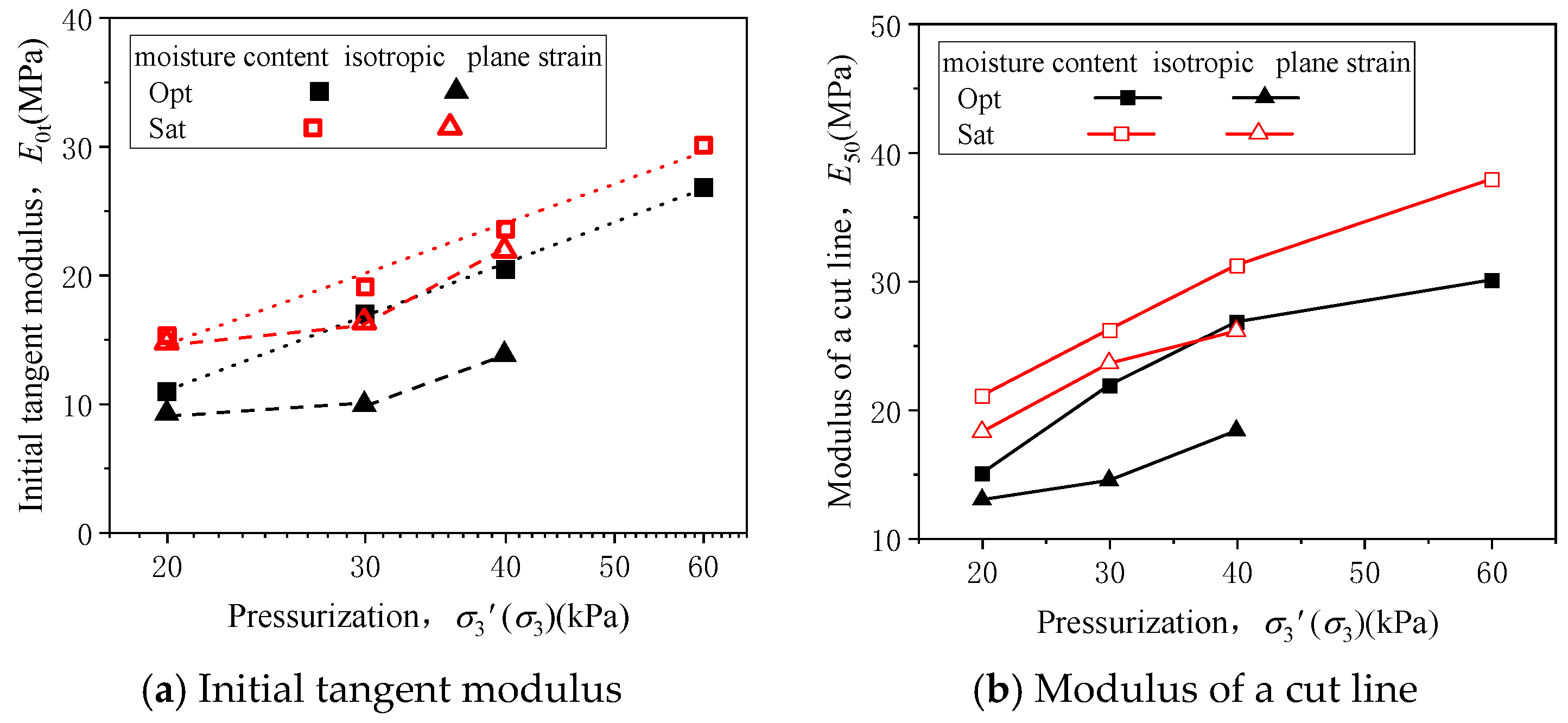
Figure 3. Gradation curve of tuff mixture.
Buildings 16 00233 g003
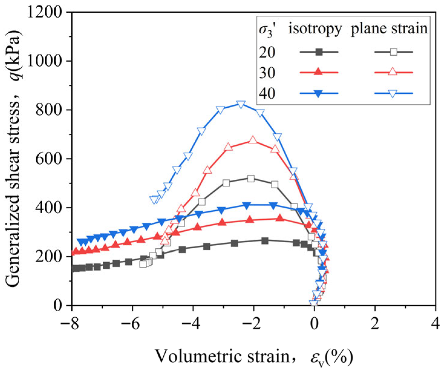
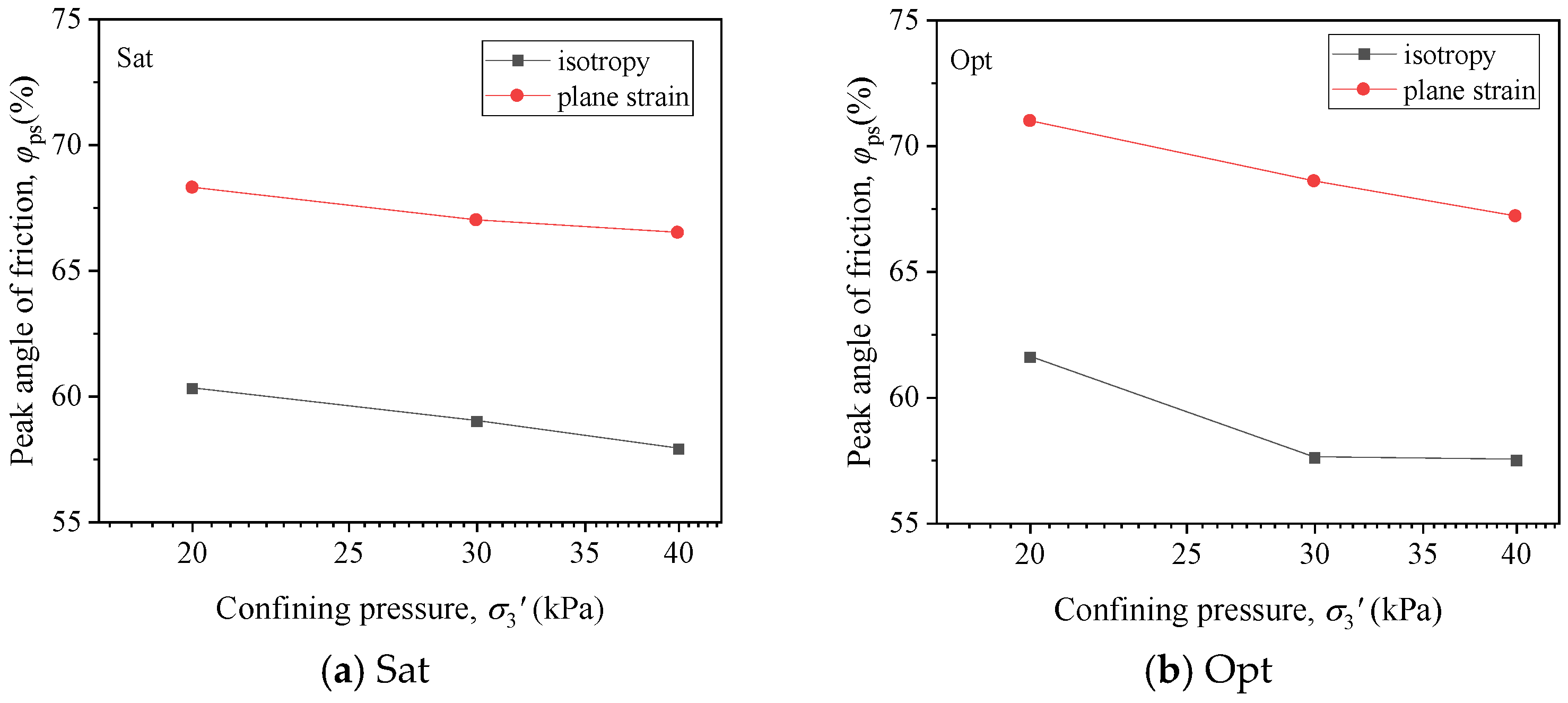
Figure 4. Sample preparation process.
Buildings 16 00233 g004
Figure 5. Schematic diagram of stress state of soil unit.
Buildings 16 00233 g005
Figure 6. Relationship between σ1 and ε1.
Buildings 16 00233 g006
Figure 7. Relationship between σ1, ps, and (σ3).
Buildings 16 00233 g007
Figure 8. Comparison of σ1 and ε1 relations under saturation and optimal water content.
Buildings 16 00233 g008
Figure 9. Relation between modulus and confining pressure.
Buildings 16 00233 g009
Figure 10. (ac) Comparison of stress–strain relationship under different drainage conditions. (d) Relation between modulus and confining pressure.
Buildings 16 00233 g010
Figure 11. Relationship between φ and ε1.
Buildings 16 00233 g011
Figure 12. Relationship between φps and σ 3 (σ3).
Buildings 16 00233 g012
Figure 13. Relationship between η and ε1.
Buildings 16 00233 g013
Figure 14. Stress path.
Buildings 16 00233 g014
Figure 15. The relationship between η/Δu and ε1.
Buildings 16 00233 g015
Figure 16. Relationship between η f and σ 3 (σ3).
Buildings 16 00233 g016
Figure 17. Relationship between σ1 and ε1.
Buildings 16 00233 g017aBuildings 16 00233 g017b
Figure 18. The relationship between σ1 and ps and its decreasing percentage and qini.
Buildings 16 00233 g018
Figure 19. Relationship between ε1, ps, and qini.
Buildings 16 00233 g019
Figure 20. Relationship between σ1, ps, and bini.
Buildings 16 00233 g020
Figure 21. Relationship between ε1, ps, and bini.
Buildings 16 00233 g021
Figure 22. Relationship between σ1, ps, and initial stress state parameters.
Buildings 16 00233 g022
Figure 23. Relationship between ε1, ps, and initial stress state parameters.
Buildings 16 00233 g023
Figure 24. Relationship between ηf and initial stress state parameters under optimal water content.
Buildings 16 00233 g024
Figure 25. Relationship between ηf and initial stress state parameters.
Buildings 16 00233 g025
Figure 26. Relationship between E50 and bini.
Buildings 16 00233 g026
Figure 27. Relationship between q and ε1.
Buildings 16 00233 g027
Figure 28. Relationship between σ and ε1.
Buildings 16 00233 g028
Figure 29. Relationship between σ1, ps, and σ 3 (σ3).
Buildings 16 00233 g029
Figure 30. Relationship between E0t and σ 3 (σ3).
Buildings 16 00233 g030
Figure 31. Relation between E50 and σ 3 (σ3).
Buildings 16 00233 g031
Figure 32. The development law of intermediate principal stress coefficient b.
Buildings 16 00233 g032
Figure 33. Relationship between σ2 and σ1.
Buildings 16 00233 g033
Figure 34. Comparison of q-ε1 curves under isotropic and plane strain conditions.
Buildings 16 00233 g034
Figure 35. Comparison of the modulus relationship between isotropy and plane strain conditions.
Buildings 16 00233 g035
Figure 36. Comparison of q-εv relations under isotropic and plane strain conditions.
Buildings 16 00233 g036
Figure 37. Comparison of φps σ 3 (σ3) relations under isotropic and plane strain conditions.
Buildings 16 00233 g037
Figure 38. Comparison of ηf σ 3 (σ3) relations under isotropic and plane strain conditions.
Buildings 16 00233 g038
Figure 39. Comparison of εvεs relations under different initial stress states.
Buildings 16 00233 g039
Figure 40. Comparison of εvεs relations under the same average principal stress but different initial stress states.
Buildings 16 00233 g040
Figure 41. Dilatancy equation fitting curve.
Buildings 16 00233 g041
Figure 42. The fitting curves of dilatancy equations under different initial stress states.
Buildings 16 00233 g042
Table 1. Generalized shear stress directions in the π-plane.
Intermediate Principal Stress Coefficient bStress Lode Angle θ (°)
0−30
0.2−19.1066
0.4−6.5868
0.66.5868
0.819.1066
Table 2. Test scheme for Coarse-Grained Soil Under Initial Isotropic Stress Conditions.
Test NameInitial Confining Pressure  σ 3 (σ3)
(kPa)
Moisture Content and Drainage ConditionsShear Rate
120Opt, Drained0.2%/min
230
340
460
520Sat, Drained
630
740
860
920Sat, Undrained
1040
1160
Table 3. Test scheme for Coarse-Grained Soil Under Three-Dimensional Initial Anisotropic Stress Conditions.
Test Namep0 (kPa)qini (kPa)biniShear Rate
Opt0.2%/min
14000
2100
30.4
40.8
5200
60.2
70.4
80.6
90.8
10300
110.2
120.4
130.6
140.8
15400
160.2
170.4
180.6
190.8
Sat0.2%/min
140100.4
2200
30.2
40.4
50.6
60.8
7300.4
8400.4
Table 4. Test scheme for Coarse-Grained Soil Under Plane Strain Conditions.
Test NameInitial Confining
Pressure  σ 3 (σ3) (kPa)
Moisture ContentShear Rate
120Opt0.2%/min
230
340
420Sat
530
640
Table 5. Fitting parameters.
Initial Generalized Shear Stress, qini (kPa)10203040
Parameters, e431.95412.18383.50368.62
Parameters, f59.1257073.358.7
Table 6. Peak friction angle and increment percentage of isotropic and plane strain tests.
Moisture ContentInitial Circumferential
Pressure
σ 3 (σ3) (kPa)
Isotropic
φtc/(°)
Plane Strain
φp/(°)
ϕ p ϕ tc ϕ tc /%
Opt2061.671.015.1
3059.268.615.9
4057.567.216.9
Sat2060.368.313.3
3058.867.013.9
4056.666.517.5
Disclaimer/Publisher’s Note: The statements, opinions and data contained in all publications are solely those of the individual author(s) and contributor(s) and not of MDPI and/or the editor(s). MDPI and/or the editor(s) disclaim responsibility for any injury to people or property resulting from any ideas, methods, instructions or products referred to in the content.