Long-Term Performance Analysis of Steel–Concrete Composite Beams Based on Finite Element Model Updating

Abstract

This study introduces a Bayesian model updating approach for analyzing the long-term performance of steel–concrete composite beams (SCBs). Two nominally identical SCBs (SCB-1 and SCB-2) were designed, fabricated, and subjected to modal testing. Despite their identical design parameters, notable differences were observed in their frequencies and mode shapes during testing. Initial finite element model (FEM) analyses, developed under testing conditions, revealed notable discrepancies between theoretically computed values and the results of modal testing. To resolve these differences, the FEM was updated using the Bayesian approach, integrating the dynamic test data to enhance model accuracy. The updated FEM was subsequently employed to assess the long-term performance of the SCBs, with a particular focus on the time-dependent effects of concrete shrinkage and creep in deflection calculations. The findings reveal substantial differences in the long-term deflection predictions between the updated and initial FEM. Specifically, the long-term deflection of SCB-1 increased by 13.1%, whereas that of SCB-2 decreased by 9.8%, leading to an overall difference of 25.3% between the two beams. These findings underscore the considerable impact of fabrication errors and material inhomogeneities on structural performance, highlighting the limitations of initial FEM based solely on test parameters in accurately capturing actual behavior. Consequently, the study emphasizes the critical role of model updating in accurately predicting the long-term performance of SCBs.

1. Introduction

Steel exhibits exceptional tensile strength, while concrete demonstrates superior performance under compressive forces. The combination of these two materials creates a synergistic effect, significantly enhancing structural efficiency. Consequently, steel–concrete composite structures have gained widespread application in bridge engineering and construction projects. Despite their advantages, steel–concrete composite beams (SCBs) are subjected to a combination of sustained loading, environmental effects, and material property degradation during their long-term service [1,2,3]. These factors introduce significant complexities in predicting their long-term behavior, posing critical challenges in the design, analysis, and maintenance of such structures.

As inherent time-dependent characteristics of concrete, creep and shrinkage have a significant impact on the performance of SCBs. Research on these phenomena has been ongoing since the early 20th century, leading to the development of numerous calculation methods and predictive models [4]. Among these, the age-adjusted effective modulus method (AEMM) [5], the CEB-FIP series of models [6], and the B3 model [7] are widely recognized. Bradford and Gilbert [8] incorporated the AEMM and interface slip effects into their analytical model, thereby enhancing the accuracy of predictions regarding the long-term performance of simply supported SCBs. Amadio and Fragiacomo [9] proposed an improved approach that integrates AEMM with concrete aging factors to refine the evaluation of creep and shrinkage behaviors. Furthermore, Sakr and Sakla [10] designed a finite element program aimed at analyzing the long-term performance of SCBs. This program incorporated a comprehensive assessment of the nonlinear displacement–slip behavior of shear connectors, concrete shrinkage and creep effects, as well as the cracking behavior of concrete slabs. Additional insights into the long-term performance of SCBs have been provided through experimental and numerical studies. Bradford and Gilbert [11], Lou et al. [12], and Wen et al. [13] offered valuable contributions, enhancing the understanding of these effects and demonstrating the importance of capturing the complex interactions involved in long-term performance assessments.

While previous studies have laid a strong theoretical foundation for understanding the long-term performance of SCBs, the inherent complexity and variable force characteristics of these structures pose significant challenges for traditional theoretical modeling and finite element analysis (FEA) methods in practical applications. On the one hand, material properties, such as the elastic modulus and time-dependent behaviors of concrete, exhibit considerable uncertainty. On the other hand, accurately characterizing the interface slip phenomenon between steel and concrete remains a challenging issue that traditional analytical methods urgently need to address. These limitations contribute to notable discrepancies between theoretical predictions and actual structural performance, thereby undermining the reliability of long-term performance assessments.

With the rapid development of the scale and design of bridge and building projects, the limitations of field measurements have become increasingly apparent. To better study the response of structures, the combination of tests and FEA has proven to be an effective tool. For instance, Lantsoght et al. [14] utilized load tests to optimize a finite element model for assessing an untestable span in a similar bridge, such as the Viaduct De Beek, thereby enabling a more thorough evaluation of the bridge’s performance. This combination of optimizations not only enhances the accuracy of the study but also has the potential to reduce the costs associated with field testing. Additionally, Domenico et al. [15] investigated the actual operational response of the bridge under both static and dynamic loads. By integrating these observations with simulations, they proposed a methodology for assessing the quality control and load-carrying capacity of the bridge deck. This approach suggests that a more comprehensive understanding and assessment of bridge performance can be achieved through the synergy of finite element analysis and actual measurements. However, when structures are composed of multiple materials, uncertainties in the finite element model (FEM) increase significantly due to factors such as manufacturing imperfections, and variability in connections between components, and material inhomogeneities [16]. These uncertainties can result in discrepancies between model predictions and actual structural performance, making it more difficult to reliably characterize the in-service behavior of the structure [17,18]. Consequently, it becomes necessary to update the FEM using measured data to ensure that the updated model reliably reflects the actual performance of the structure. This process is known as Finite Element Model Updating (FEMU).

According to the type of measurement data, FEMU methods are typically categorized into two main types: dynamic updating and static updating methods [19]. Compared to static updating methods, dynamic model updating methods provide richer structural response information, such as frequency response function, natural frequencies, mode shapes, and mode strain energy. Additionally, dynamic methods do not require loading the structure and can be performed without disrupting the normal use of the structure. As a result, they have increasingly become a focal point of research in recent years [19,20,21,22]. FEMU is fundamentally a mathematical inverse problem, with the primary goal of inferring structural parameters based on observed response data. This process is typically formulated as a constrained optimization problem that minimizes the difference between the computational results of the model and the observed data. However, in practice, these optimization problems are often ill-posed, meaning that the inverse solution may not consistently exhibit assured uniqueness and stability, thereby compromising the robustness and practical applicability of FEMU methods. The Bayesian approach has proven effective in addressing the ill-posed nature of model updating inverse problems by incorporating a probabilistic framework into the parameter space [23,24,25,26]. For instance, Ching et al. [25] introduced a Bayesian model updating (BMU) approach for linear elastic structures that accounts for parameter uncertainty and handles incomplete observed data through a Gibbs sampling algorithm. Applied to a three-dimensional frame structure and a shear structure, this method not only achieved model updating but also successfully identified the location and extent of structural damage. Furthermore, Christodoulou and Papadimitriou [26] proposed a structural model updating method that integrates measured modal data with the minimization of weighted residuals within a Bayesian framework and demonstrated its effectiveness through a numerical example. Despite the success of these methods in engineering applications, significant challenges remain. Some approaches require repetitive finite element computations, which are very time-consuming, while others require solving ill-conditioned model updating equations, inevitably encountering ill-posed inverse problems, in multiple or unstable solutions [17].

To address the issue of time-consuming computations, Chen et al. [21] proposed a Bayesian Markov Chain Monte Carlo model updating method with a homotopy surrogate model. This approach efficiently approximates the vibration mode and frequency data of the structure, enabling the rapid updating of structural parameters. Its effectiveness and accuracy were demonstrated in an engineering case study involving a large cable-stayed bridge. In terms of mitigating the ill-posed nature of model updating, Chen et al. [22] developed an FEMU algorithm that utilizes an improved cross-model cross-mode method to simultaneously update structural mass and stiffness. And the effectiveness of this method was confirmed through a modal test of a cantilever beam. Yuen, meanwhile, introduced a BMU method based on iterative optimization [23,24,27,28,29]. This method calculates the partial derivatives of the fitting function and iteratively estimates the most likely values of the structural response and structural parameters. The Hessian matrix is then used to directly estimate the uncertainty of the modification coefficients. A key advantage of the approach is that it can avoid lengthy finite element computations and ill-posed inverse problems. This makes it particularly reliable for updating high-dimensional parameters.

To improve the accuracy and reliability of predicting the long-term performance of SCBs, this study employs a BMU based on optimizing partial derivatives to update structural parameters. For SCBs, key factors, such as the slip characteristics at the interface and the elastic modulus of the materials, play a significant role in influencing their long-term deflection. Considering that only low-order frequency and modal data are available in the modal testing of SCBs, this study aims to update the FEM of SCBs using limited measurement data. Based on the updated models, the long-term performance of the SCBs is comprehensively analyzed.

The organization of this paper is as follows. Section 2 reviews the underlying theory for the finite element analysis concerning the long-term behavior of SCBs. Section 2 introduces the theoretical foundation pertaining to finite element analysis of the long-term behavior of SCBs. Section 3 outlines the principles of the Bayesian method along with the model reduction approach used for updating SCBs. 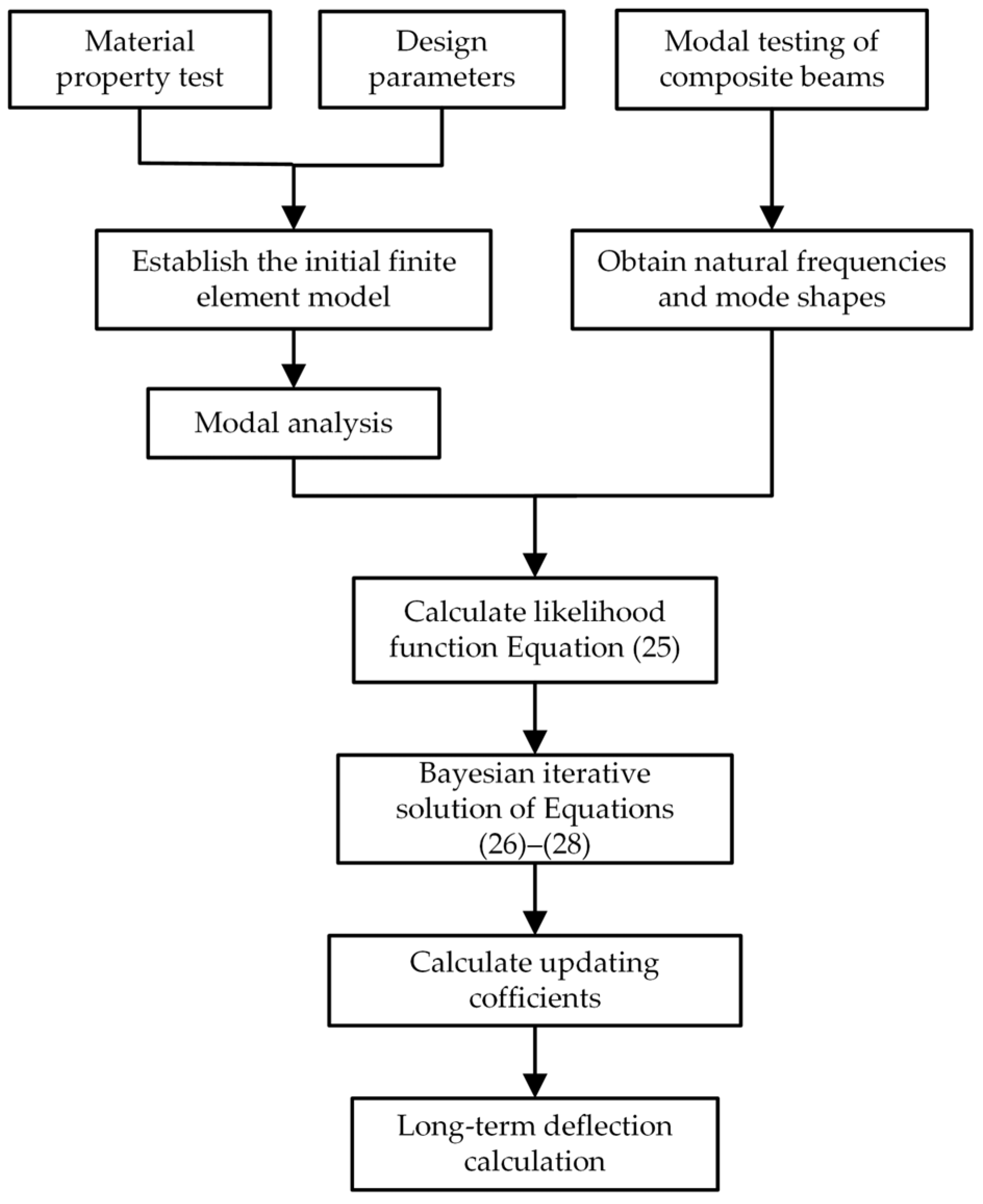Section 4 details the process of the proposed method and its associated workflow. Section 5 presents the results of modal testing and FEMU for the SCBs. Section 6 investigates the long-term performance based on the updated FEM of the SCBs. Finally, Section 7 presents the main conclusions.

2. Finite Element Theory

2.1. Design of Specimens

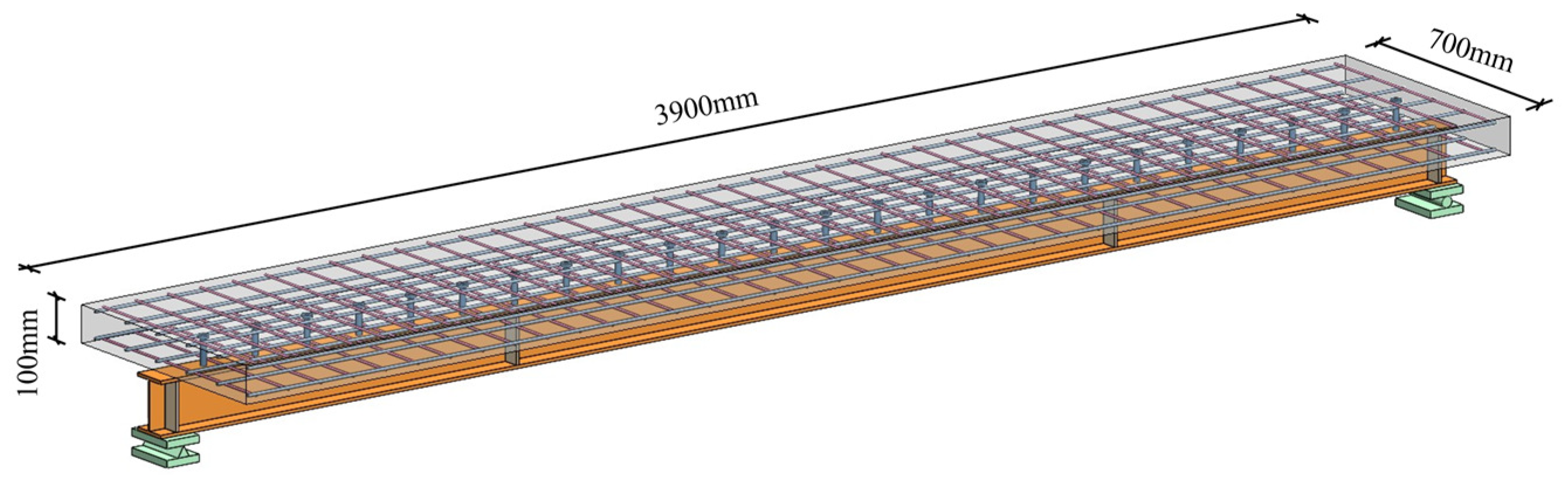
In this study, two SCBs with identical parameters were designed and fabricated, designated as SCB-1 and SCB-2. Both specimens were constructed with a full shear connection, achieving the synergistic interaction between the concrete slab and steel beam through the use of shear studs. This connection technique facilitates the coordinated transfer of forces between the two components. The overall structural configuration of the specimens is illustrated in Figure 1.

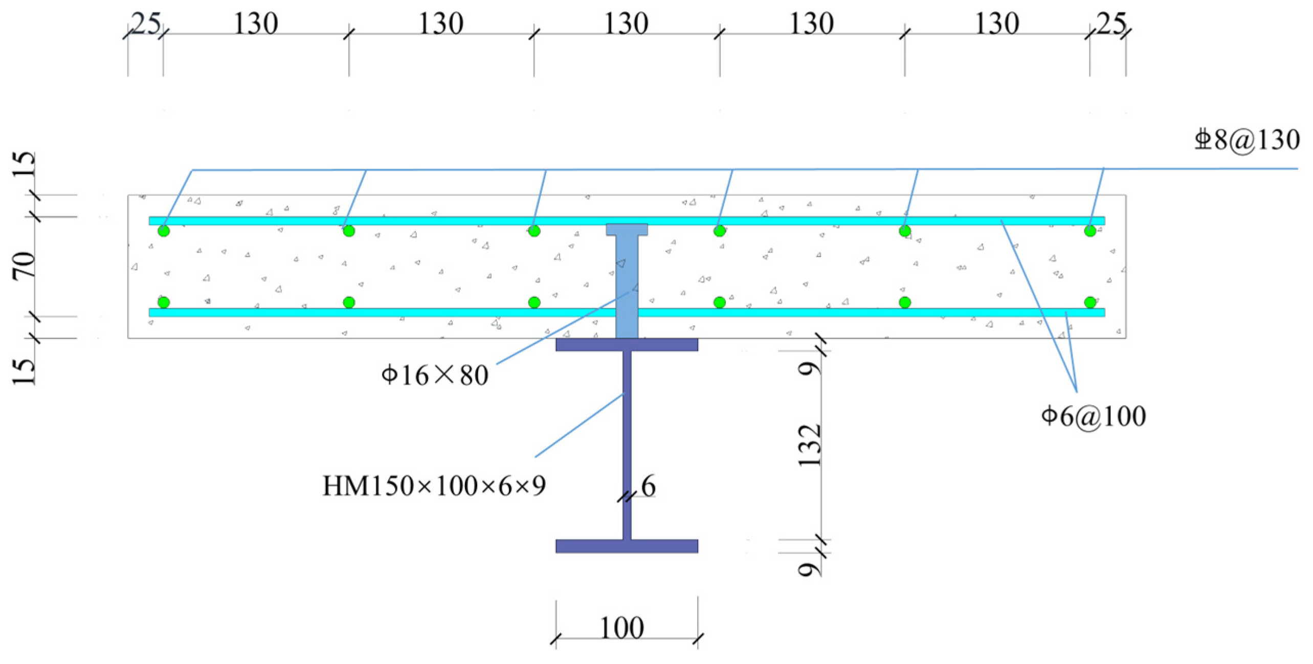
The main design parameters of the test specimens were as follows: the effective span of each test specimen was 3900 mm, with a total section height of 250 mm. The concrete flange plate was cast in place using C40 concrete, featuring a width of 700 mm and a thickness of 100 mm. Detailed dimensions and parameters for each component of the specimen are presented in Figure 2. To ensure overall load-bearing performance and to prevent local instability, 8 mm thick Q235 steel stiffeners were welded at critical locations, including near the supports and at the mid-span.

Accurately selecting appropriate material models for steel and concrete is essential for ensuring the reliability of finite element analysis results when assessing the long-term performance of SCBs. This analysis was conducted using the nonlinear finite element software ABAQUS 2022/Standard 6.10, with appropriate parameters set to accurately describe the material properties and mechanical behavior of each component.

2.2. Cell Types and Meshing

In the finite element modeling process, appropriate element types are chosen for various structural components to accurately represent their mechanical properties. The concrete slab and shear connectors were modeled using eight-node linear solid elements (C3D8), while the steel beams were represented with four-node shell elements (S4). This approach enhances the computational efficiency while accurately capturing the mechanical behavior of thin-walled structures. The internal reinforcements were modeled with double-node truss elements (T3D2), which are particularly suitable for simulating axial force behavior.

A non-uniform grid strategy was employed during mesh generation to optimize the balance between computational accuracy and efficiency. The mesh sizes of each component were meticulously adjusted: 20 mm mesh sizes were applied to the steel beam and reinforcements, 50 mm mesh sizes were employed for the concrete slabs, and fine 5 mm mesh sizes were utilized for shear connectors to more accurately capture their intricate mechanical behavior.

2.3. Interaction and Boundary Conditions

The interaction among the various components of the SCBs is a key factor influencing its mechanical performance. To accurately capture the interface behavior within the numerical model, a detailed interface contact relationship was established. Furthermore, to simplify the model while accurately reflecting real-world conditions, the boundary conditions were carefully defined based on the actual constraints of the SCBs. The specific interface contact relationships and boundary condition configurations are presented in detail in Figure 3.

2.4. Load

To accurately simulate the mechanical behavior of SCBs under real-world working conditions, a uniformly distributed load was applied across the entire span on the surface of the concrete slab. These loads were configured to simulate the cumulative effects of both dead and live loads, which are typical of the actual working conditions encountered by SCBs in structural applications.

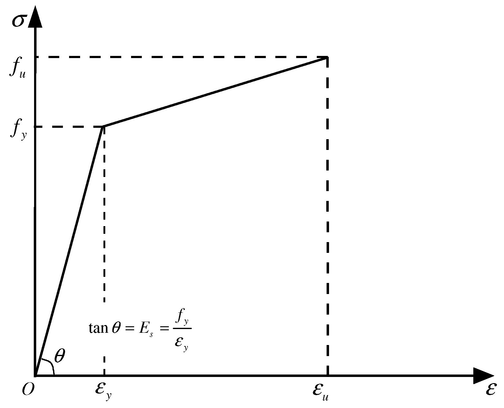
2.5. Steels

The steel components were modeled using a bilinear hardening principle, incorporating the Von Mises yield criterion to define the onset of plastic behavior. A tangent modulus of E_t = 0.01 E_s was assigned to capture the material’s strain-hardening phase accurately. The detailed stress–strain relationship is illustrated in Figure 4.

2.6. Concrete

To accurately simulate the complex mechanical behavior of concrete in SCBs, this study employed a multi-scale material simulation framework. The framework integrates the concrete damage plasticity (CDP) model and incorporates specialized FORTRAN subroutines to simulate the creep and shrinkage behavior of concrete. By coupling these subroutines with the plastic damage analysis module, the framework effectively captures the long-term performance of SCBs under sustained loads.

The uniaxial tensile and compressive behavior of concrete was modeled in accordance with GB50010-2010 [30]. The primary parameters used for implementing the CDP model in ABAQUS are shown in

Table 1. Primary parameters for the CDP model.

Dilation Angle (ψ)	Eccentricity (ξ)	fb0/fc0	Kc	μ
35	0.1	1.16	0.6667	0.0005

.

2.6.1. Creep Model

To achieve a more precise simulation of concrete creep behavior under long-term loading, this study employed the linear viscous transformation theory. According to the superposition principle and the assumption of a linear creep model, the total strain of concrete is divided into three components:

$$\epsilon (t)={\epsilon }^e(t)+{\epsilon }^c(t)+{\epsilon }^{sh}(t)$$

(1)

where ${\epsilon }^e(t)$ is the instantaneous elastic and plastic strain of concrete, ${\epsilon }^c(t)$ is the creep strain of concrete, and ${\epsilon }^{sh}(t)$ is the shrinkage strain of concrete.

The creep behavior of concrete is commonly characterized by the creep coefficient $\varphi \left(t,\tau \right)$, which quantifies the gradual increase in strain over time under constant stress. As defined by the American ACI 209 model [31], the creep strain of concrete can be expressed as:

$${\epsilon }^c(t,\tau )={\displaystyle \frac{\sigma (\tau )}{E}}\varphi \left(t,\tau \right)$$

(2)

where $\sigma \left(\tau \right)$ is the stress value at the loading moment $\tau$.

In the analysis of the creep model, two key parameters are central to describing the time-dependent deformation of concrete: the creep degree function $C\left(t,\tau \right)$ and the creep function $J\left(t,\tau \right)$. The relationship between these two parameters is expressed as follows:

$$C(t,\tau )={\displaystyle \frac{\varphi (t,\tau )}{E}}$$

(3)

$$J(t,\tau )={\displaystyle \frac{1+\varphi (t,\tau )}{E}}$$

(4)

The concrete creep behavior is governed by a range of factors, including intrinsic material properties, member dimensions, curing conditions, external environmental influences (e.g., temperature and humidity), and the stress history of the structure. These complexities make modeling and analyzing creep effects a challenging task. To address these intricacies, this study employed the step-by-step integration method for calculating creep effects in structures. This numerical approach divides the time domain into discrete intervals to incrementally evaluate the cumulative creep strain, accommodating changes in stress, environmental conditions, and time-dependent material properties. The process is illustrated in Figure 5, providing a clear framework for assessing the long-term effects of creep in complex structural systems.

Throughout the duration of creep, the general expression for concrete creep strain is derived to represent the time-dependent deformation under sustained loading. This expression is conventionally defined as:

$$\left\{{\epsilon }^c\left(t\right)\right\}=\left[A\right]\left\{\Delta {\sigma }_0\right\}C\left(t,t_0\right)+{\displaystyle {\int }_{t_0}^{t}C\left(t,\tau \right)\left[A\right]\left\{\frac{d\sigma }{d\tau }\right\}d\tau }$$

(5)

where [A] is the transformation matrix that accounts for the effect of Poisson’s ratio:

$$\left[A\right]=\left[\begin{array}{cccccc}1& -\mu & -\mu & 0& 0& 0\\ & 1& -\mu & 0& 0& 0\\ & & 1& 0& 0& 0\\ & & & 2(1+\mu )& 0& 0\\ & & & & 2(1+\mu )& 0\\ & & & & & 2(1+\mu )\end{array}\right]$$

(6)

The entire process of creep analysis can be segmented into a series of discrete time intervals ($\Delta t_1,\Delta t_2,\Delta t_3,\dots ,\Delta t_n$), enabling the calculation of strain increments for each interval. The creep strain increment during a given time interval $\Delta t_n$ is expressed as:

$$\left\{\Delta {\epsilon }_{\mathrm{n}}^c\right\}=\left\{{\epsilon }^c\left(t_n\right)\right\}-\left\{{\epsilon }^c\left(t_{n-1}\right)\right\}=[A]{\displaystyle {\int }_{t_{n-1}}^{t_n}C\left(t,\tau \right)\frac{d\sigma }{d\tau }d\tau }$$

(7)

If the time interval is chosen to be sufficiently small such that the stress change remains constant within the time interval $\Delta t_n$, the integral expression in Equation (7) can be expressed as

$$\left\{\Delta {\epsilon }_{\mathrm{n}}^c\right\}=[A]C\left(t,t_{n-0.5}\right)\left\{\Delta {\sigma }_n\right\}$$

(8)

where $\left\{\Delta {\sigma }_n\right\}$ is the stress increment.

The creep strain increment $\left\{\Delta {\epsilon }^c(t_{n+1})\right\}$ of concrete from moment n to moment n + 1 can be calculated as

$$\left\{\Delta {\epsilon }^c(t_{n+1})\right\}=[A]\left[\begin{array}{l}\left\{{\epsilon }^c(t_{n+1})\right\}-\left\{{\epsilon }^c(t_n)\right\}=[C(t_{n+1},t_0)-C(t_n,t_0)]\left\{\Delta {\sigma }_0\right\}\\ +[C(t_{n+1},t_{1-0.5})-C(t_n,t_{1-0.5})]\left\{\Delta {\sigma }_1\right\}+\dots \\ +[C(t_{n+1},t_{n-0.5})-C(t_n,t_{n-0.5})]\left\{\Delta {\sigma }_n\right\}+C(t_{n+1},t_{n+1-0.5})\left\{\Delta {\sigma }_{n+1}\right\}\end{array}\right]$$

(9)

To improve computational efficiency, a step-by-step integral calculation approach based on the Dirichlet series was employed. In this method, $C\left(t,\tau \right)$ is expressed as a Dirichlet series [32]:

$$C(t,\tau )={\displaystyle \sum _{i=1}^m{a}_i(\tau )[1-e^{-{\lambda }_i(t-\tau )}]}$$

(10)

In Equation (10), m = 4 is taken to improve the accuracy of the calculation, and ${\lambda }_i$ is taken as 1, 0.1, 0.01, and 0.001; $a_i(\tau )$ is the coefficient to be determined based on least-squares fitting.

It can be obtained from Equation (10):

$$\begin{array}{l} C(t_{n+1},t_{i-0.5})-C(t_n,t_{i-0.5})={\displaystyle \sum _{j=1}^m{a}_j(t_{i-0.5})[1-e^{-{\lambda }_j(t_{n+1}-t_{i-0.5})}]}-{\displaystyle \sum _{j=1}^m{a}_j(t_{i-0.5})[1-e^{-{\lambda }_j(t_n-t_{i-0.5})}]}\\ ={\displaystyle \sum _{j=1}^m{a}_j(t_{i-0.5})e^{-{\lambda }_j(t_n-t_{i-0.5})}[1-e^{-{\lambda }_j\Delta t_{n+1}}]}\end{array}$$

(11)

Based on this expansion, the concrete creep strain increment $\left\{\Delta {\epsilon }^c(t_{n+1})\right\}$ in Equation (9) can be re-expressed as

$$\left\{\Delta {\epsilon }^c(t_{n+1})\right\}={\displaystyle \sum _{j=1}^m\left\{g_j(t_{n+1})\right\}[1-e^{-{\lambda }_j\Delta t_{n+1}}]}+[A]C(t_{n+1},t_{n+1-0.5})\left\{\Delta {\sigma }_{n+1}\right\}$$

(12)

where the recurrence relation for the intermediate variable $\left\{g_j(t_{n+1})\right\}$ is:

$$\left\{g_j(t_{n+1})\right\}=\left\{g_j(t_n)\right\}{e}^{-{\lambda }_j\Delta t_n}+[A]\left\{\Delta {\sigma }_n\right\}{a}_j(t_{n-0.5})e^{-0.5{\lambda }_j\Delta t_n}$$

(13)

2.6.2. Shrinkage Model

In this study, the shrinkage deformation of concrete, which is less complex than creep due to its independence from applied stress, was estimated using the shrinkage model provided in JTG 3362-2018 [33]. The corresponding shrinkage strain is expressed as:

$${\epsilon }^{sh}(t,t_s)={\epsilon }_{cso}{\beta }_s(t-t_s)$$

(14)

where

$${\epsilon }_{cso}={\epsilon }_s(f_{cm}){\beta }_{RH}$$

(15)

$${\beta }_{RH}=1.55[1-{\left(RH/100\%\right)}^3]$$

(16)

$${\epsilon }_s(f_{cm})=[160+100{\beta }_{sc}(9-f_{cm}/10)]·{10}^{-6}$$

(17)

$${\beta }_s(t-t_s)=\sqrt{{\displaystyle \frac{t-t_s}{t-t_s+350{(h/100)}^2}}}$$

(18)

In the above equation, $t$ and $t_s$ represent the age of the concrete at the time of calculation and the age of the concrete at the onset of shrinkage, respectively. ${\epsilon }^{sh}(t,t_s)$ is the shrinkage strain. ${\epsilon }_{cso}$ is the nominal shrinkage coefficient. ${\beta }_s$ is the coefficient describing the development of shrinkage over time, ${\beta }_{sc}$ is determined based on the type of cement used. $f_{cm}$ and $f_{cu}$ correspond to the average cylinder compressive strength and the standardized cubic compressive strength (MPa), respectively. ${\beta }_{RH}$ represents the coefficient associated with the annual average relative humidity. $RH$ refers to the annual average relative humidity (%) of the environment.

2.7. Calculation Program

To account for the long-term behavior of SCBs, this study leveraged the large-scale finite element software ABAQUS, incorporating three user-defined subroutines—USDFLD, GETVRM, and UEXPAN—for the customized development of material properties. Specifically, the USDFLD subroutine was employed to update the field variables at the integration points, dynamically capturing the time-dependent variations in the elastic modulus of concrete. The GETVRM subroutine enhanced the precision of the creep analysis by extracting stress and strain data at material points, enabling the effective coupling of stress states within the simulation. Meanwhile, the UEXPAN subroutine calculated the creep and shrinkage strain increments at each time step and integrates these effects into the main program, ensuring the robust modeling of time-dependent phenomena. Additionally, the CDP model was employed in the elasto-plastic analysis to capture the plastic damage behavior of concrete. Together, the main program and these subroutines constitute a comprehensive numerical simulation framework for analyzing the concrete shrinkage and creep behavior.

3. Theory of Model Updating

3.1. Bayesian Approach for Dynamic Model Updating

Assuming that the mass of the SCB is known, the actual eigenvalue equation for the SCB can be represented as

$$\mathbf{K}(\mathit{\alpha }){\mathit{\psi }}_e={\displaystyle \sum _{i=1}^l{\alpha }_i}{K}_i{\mathit{\psi }}_e={\mathit{\lambda }}_e\mathbf{M}{\mathit{\psi }}_e$$

(19)

where $K(\mathit{\alpha })$ denotes the stiffness matrix; $K_i$ represents the stiffness matrix of the i-th region. $\mathbf{M}$ represents the mass matrix. $\mathit{\alpha }$ is the vector of updating parameters, $\mathit{\alpha }={[{\alpha }_1,{\alpha }_2,\cdots {\alpha }_l]}^T$, and l is the number of updating parameter. It is assumed that the N-th order modes and eigenvalues of the system $\mathit{R}$ are measured, with ${\mathit{\lambda }}_e$ denoting the eigenvalue and ${\mathit{\lambda }}_e={[{\lambda }_1,{\lambda }_2,\cdots {\lambda }_N]}^T$. ${\mathit{\psi }}_e$ is the corresponding vibration modes, and ${\mathit{\psi }}_e=[{\mathit{\psi }}_1,{\mathit{\psi }}_2,\cdots ,{\mathit{\psi }}_N{]}^T$.

The objective of BMU is to refine the posterior probability distribution of the parameter $\mathit{\alpha }$ using the observed data $\mathit{Z}$, as defined by the following expression:

$$p(\mathit{\alpha },\mathit{\lambda },\mathit{\psi }/\mathit{Z},\mathit{R})\propto p(\mathit{Z}/\mathit{\alpha },\mathit{\lambda },\mathit{\psi },\mathit{R})p(\mathit{\alpha }/\mathit{R})p(\mathit{\lambda },\mathit{\psi }/\mathit{\alpha },\mathit{R})$$

(20)

where $\mathit{Z}=\left\{{\mathit{\lambda }}_e,{\mathit{\psi }}_e\right\}$ represents the actual observed data. The likelihood function is represented by $p(\mathit{Z}/\mathit{\alpha },\mathit{\lambda },\mathit{\psi },\mathit{R})$, and the prior probability distribution of the structural updating parameters is represented by $p(\mathit{\alpha }/\mathit{R})$. In this study, this prior was assumed to be a Gaussian distribution with mean ${\mathit{\alpha }}^o$ and covariance matrix ${\mathbf{\Sigma }}_{\mathit{\alpha }}$. Additionally, $p(\mathit{\lambda },\mathit{\psi }/\mathit{\alpha },\mathit{R})$ denotes the prior joint distribution of the modal vector and structural updating coefficient vector.

The consideration of errors between the measured and calculated data is expressed as:

$${\mathit{\lambda }}_e=\mathit{\lambda }+{ϵ}_{\mathit{\lambda }},\hspace{1em}{\mathit{ϵ}}_{\mathit{\lambda }}\sim \mathcal{N}(0,{\sigma }_{\mathit{\lambda }}^2)$$

(21)

$${\mathit{\psi }}_e={\mathbf{L}}_0\mathit{\psi }+{\mathit{ϵ}}_{\mathit{\psi }},\hspace{1em}{\mathit{ϵ}}_{\mathit{\psi }}\sim \mathcal{N}(0,{\sigma }_{\mathit{\psi }}^2\mathit{I})$$

(22)

where $\mathit{\lambda }$ denotes the eigenvalue obtained from the initial FEM analysis, and ${\mathit{ϵ}}_{\mathit{\lambda }}$ represents the eigenvalue error, which was assumed to follow a normal distribution with a mean of zero. ${\mathbf{L}}_0$ is the observation matrix for the mode shape, which maps the global mode DOF from the FEM to the observed DOF. ${\mathit{ϵ}}_{\mathit{\psi }}$ corresponds to the error in the mode shape and was presumed to adhere to a zero-mean Gaussian distribution. Consequently, the likelihood function is defined in the following manner:

$$p\left({\mathit{\lambda }}_e,{\mathit{\psi }}_e|\mathit{\alpha },\mathit{\lambda },\mathit{\psi },\mathit{R}\right)\propto exp(-{\displaystyle \frac{1}{2}}{‖\mathit{\psi }-{\mathbf{L}}_0{\mathit{\psi }}_e‖}_{{\mathbf{\Sigma }}_{\psi }^{-1}}^2-{\displaystyle \frac{1}{2}}{‖{\mathit{\lambda }}_e-\mathit{\lambda }‖}_{{\mathbf{\Sigma }}_{\lambda }^{-1}}^2)$$

(23)

where $‖·‖$ denotes the Euclidean paradigm, and the ${\mathbf{\Sigma }}_{\psi }$ and ${\mathbf{\Sigma }}_{\lambda }$ represent the covariance matrices corresponding to the mode shape and eigenvalue, respectively.

Based on Bayesian theorem, the posterior probability density function of unknown parameters can be represented as

$$p(\mathit{\alpha },\mathit{\lambda },\mathit{\psi }/\mathit{Z},\mathit{R})={\mathit{\kappa }}_1\left(-{\displaystyle \frac{1}{2}}J(\mathit{\alpha },\mathit{\lambda },\mathit{\psi })\right)$$

(24)

where ${\mathit{\kappa }}_1$ represents the unknown normalization constant, and $J(\mathit{\alpha },\mathit{\lambda },\mathit{\psi })$ is the fitting function, which is defined as follows:

$$J(\mathit{\alpha },\mathit{\lambda },\mathit{\psi })=\left\{\left.\begin{array}{l}{\displaystyle \frac{1}{{\sigma }_e^2}}{\displaystyle \sum _{n=1}^N{‖\left(K(\mathit{\alpha })-{\lambda }_{n}M\right){\psi }_n‖}^2}+{\left[\begin{array}{c}{\mathit{\lambda }}_e-\mathit{\lambda }\\ \mathit{\psi }-L_o{\mathit{\psi }}_e\end{array}\right]}^T{\mathbf{\Sigma }}_{\mathit{ϵ}}^{-1}\left[\begin{array}{c}{\mathit{\lambda }}_e-\mathit{\lambda }\\ \mathit{\psi }-L_o{\mathit{\psi }}_e\end{array}\right]\\ +{(\mathit{\alpha }-{\mathit{\alpha }}^o)}^T{\mathbf{\Sigma }}_{\mathit{\alpha }}^{-1}(\mathit{\alpha }-{\mathit{\alpha }}^o)\end{array}\right\}\right.$$

(25)

where ${\sigma }_e^2$ is the error variance.

We calculated the partial derivatives of updating coefficients and modal parameters for Equation (25) separately and iterated:

$${\psi }^{\star }=\arg {\min }_{\psi }J({\lambda }^{\star },\psi ,{\alpha }^{\star })$$

(26)

$${\lambda }^{\star }=\arg {\min }_{\lambda }J(\lambda ,{\psi }^{\star },{\alpha }^{\star })$$

(27)

$${\alpha }^{\star }=\arg {\min }_{\alpha }J({\lambda }^{\star },{\psi }^{\star },\alpha )$$

(28)

The detailed calculation procedure of Equations (26)–(28) can be found in the literature [23]. After a set number of iterations (usually in the hundreds), ${\alpha }^{\star }$ in Equations (26)–(28) represents the most probable value of the updating coefficient.

3.2. Dynamic Model Reduction

During model updating, discrepancies frequently arise between the degrees of freedom (DOFs) represented in the FEM and those captured through experimental dynamic measurements. These discrepancies are primarily due to sensor limitations, as experimental tests typically provide vibration data for only a subset of the structural DOFs. This constraint prevents a full characterization of the dynamic response of the structure. To address this limitation, dynamic model reduction techniques are employed to condense the DOFs in the equations of motion, ensuring compatibility with the available measured data. By doing so, the eigenvalue problem of the structure can be reformulated into the following decomposed form [34]:

$$\left[\begin{array}{cc}{K}_{hh}& K_{hg}\\ K_{gh}& K_{hh}\end{array}\right]\left[\begin{array}{c}{\psi }_h\\ {\psi }_g\end{array}\right]=\lambda \left[\begin{array}{cc}{M}_{hh}& M_{hg}\\ M_{gh}& M_{gg}\end{array}\right]\left[\begin{array}{c}{\psi }_h\\ {\psi }_g\end{array}\right]$$

(29)

where h represents the number of measured DOFs, while g denotes the unmeasured ones, with the total number of global DOFs being h + g = N. ${\psi }_h$ and ${\psi }_g$ correspond to the vibrational components of mode shape for the measured and unmeasured DOFs, respectively.

The influence of the unmeasured DOFs can be incorporated into the measured DOFs by processing the partitioned eigenvalue equations, as detailed in [34]:

$$K_{hh}{\psi }_h+K_{hg}{\psi }_g={\omega }^2(M_{hh}{\psi }_h+M_{hg}{\psi }_g)$$

(30)

$$K_{gh}{\psi }_h+K_{gg}{\psi }_g={\omega }^2(M_{gh}{\psi }_h+M_{gg}{\psi }_g)$$

(31)

In the dynamic model reduction process, this paper adopted the iterative improved reduction system technique to solve Equations (30) and (31), thereby enhancing the accuracy of the reduction procedure. The recursive formula for the transformation matrix is expressed as follows:

$${\mathbf{\Lambda }}_j={\mathbf{\Lambda }}_{j-1}-{\mathbf{\Lambda }}_{j-1}{M}_{gg}^{-1}(M_{gh}{\mathbf{\Lambda }}_{j-1})$$

(32)

where ${\mathbf{\Lambda }}_0=I$.

By iteratively applying Equation (32), with $K_h$ and $M_h$ corresponding to the measured DOFs, h can be computed as follows:

$${\mathbf{\Lambda }}_h={\mathbf{\Lambda }}_j^{T}K{\mathbf{\Lambda }}_j$$

(33)

$$M_h={\mathbf{\Lambda }}_j^{T}M{\mathbf{\Lambda }}_j$$

(34)

Similarly, the stiffness matrix $K_{ej}$ and mass matrix $M_{ej}$ for the j-th element or region within the global DOFs of the structure can be represented using the following expressions:

$$K_{e_j}={\mathbf{\Lambda }}_j^T{K}_e{\mathbf{\Lambda }}_j$$

(35)

$$M_{ej}={\mathbf{\Lambda }}_j^T{M}_e{\mathbf{\Lambda }}_j$$

(36)

In practical calculations, to ensure high accuracy in the dynamic model reduction process, the number of iterations j was set to 1 in this study.

4. Main Steps and Flowchart

The proposed methodology was implemented through a series of systematic steps. Initially, the material properties of the SCBs were determined through experimental testing. Subsequently, modal testing was conducted to acquire their natural frequencies and mode shape data. Based on these findings, an initial FEM was developed utilizing the design parameters along with the experimentally measured material characteristics. Modal analysis was performed on this initial FEM to compute theoretical frequencies and mode shapes, allowing a comparison between the calculated results and experimental measurements. Within the Bayesian framework, updating coefficients were defined according to a Gaussian prior distribution. Utilizing the experimentally measured dynamic data, a likelihood function was constructed, as detailed in Equation (25). The optimal updating coefficients were iteratively determined by solving Equation (25). Finally, the long-term deflection behavior of the SCBs was simulated using the updated FEM. To validate the significance of the model updating process, the results from the updated model were compared to those of the initial FEM, demonstrating the necessity of model refinement for accurate long-term performance evaluations. A schematic representation of the proposed methodology is provided in Figure 6.

5. Modal Testing and Model Updating Results

5.1. Material Properties

5.1.1. Concrete Material

The specimens were constructed using concrete classified as C40. Three specimens, each measuring 150 mm × 150 mm × 150 mm, were concurrently produced during the casting process to assess the cubic compressive strength of the concrete. Additionally, six specimens with the dimensions of 150 mm × 150 mm × 300 mm were fabricated to evaluate their axial compressive strength and modulus of elasticity. All specimens cured under standard environmental conditions for 28 days.

Table 2. Basic mechanical properties of concrete.

Concrete Strength Grade	Cubic Compressive Strength (fcu)/MPa	Axial Compressive Strength (fc)/MPa	Elasticity Modulus (Ec)/MPa
C40	48.6	37.97	3.73 × 104

presents the basic mechanical properties of the concrete.

5.1.2. Steel

In accordance with the standard GB/T 2975-2018 [35], three specimens were taken from the web and flange of the steel beam, as well as the embedded reinforcement, for mechanical property testing. The results of these tests are summarized in

Table 3. Mechanical properties of steel.

Type of Steel		Thickness (Diameter)/mm	Yield Strength (fy)/MPa	Ultimate Tensile Strength (fu)/MPa	Elongation After Fracture/%
Steel beam	Web	6	356.77	518.16	20.811
	Flange	9	374.88	530.77	17.09
Steel reinforcement	longitudinal	8	505.43	590.69	19.31
	transverse	6	513.16	532.05	7.62

.

5.1.3. Shear Connectors

The specimens were equipped with shear connectors in the form of Φ16 × 80 studs, with their mechanical properties obtained from the factory quality inspection report. The key parameters were as follows: yield strength of 350 MPa, tensile strength of 450 MPa, and elongation of 18.2%.

5.2. Modal Testing

The modal testing of the SCBs was performed using the operational modal analysis method. Fifteen points for capturing vertical vibrations were systematically arranged along the beam span. The outermost point positioned 270 mm from the beam end, and a uniform spacing of 240 mm between adjacent points. The arrangement of measurement points is depicted in Figure 7. Before testing, a laser displacement sensor was used to verify the support constraints, ensuring that the actual boundary conditions matched the design specifications and minimizing any potential influence on the test results.

During the experiment, five IEPE piezoelectric accelerometers were employed to collect data simultaneously. The technical specifications of these accelerometers include a sensitivity of 11.05 mV/g, a measurement range of ±500 g, and a frequency response range of 0.5–3000 Hz. Every accelerometer was firmly fastened to the surface of the SCBs at the specified measurement points using a magnetic base. Prior to testing, the amplitude and phase of the accelerometers were carefully calibrated to ensure data acquisition accuracy and consistency.

The excitation method for modal testing adopted random excitation. The experimental setup involved dividing the SCBs into four distinct sampling groups, with a consistent reference accelerometer employed across all groups to seamlessly “glue” the different mode shapes. The acceleration data collected during testing were analyzed using the Enhanced Frequency Domain Decomposition method [36]. Figure 8 depicts the specific process of modal testing, while Figure 9 and Figure 10 present the extracted mode shapes and their corresponding natural frequencies, respectively.

5.3. Model Updating

To more accurately capture the localized distribution characteristics of the material properties in the SCBs, this study divided the FEM of the SCBs into multiple zones and update the parameters of each region. The FEM was divided into 16 regions, with the specific zoning scheme illustrated in Figure 11. To consider the variability in material characteristics during casting, the upper concrete slab was partitioned into 10 distinct regions. Similarly, due to variability introduced during the fabrication of the bottom steel girder, it was uniformly segmented into five regions along its length. Moreover, considering the complex interactions between the steel and concrete layers [37,38], the bond slip mechanism at their interface is crucial to the overall response of SCBs. Drawing on the bonded interface characteristics of SCBs elements proposed by Sadeghi et al. [39], the stiffness parameter (bond coefficient) of the steel–concrete interface was revised in this study.

Consequently, three key parameters were selected for the updating process: the elastic modulus of each concrete slab segment, the flexural stiffness of each steel beam segment, and the bond coefficient at the steel–concrete interface. To streamline the updating and analysis, updating coefficients were defined as the ratios of these parameters to their initial values, resulting in a total of 16 updating coefficients. This zoned approach enhances the flexibility and localization of parameter identification while maintaining the accuracy and efficiency of the updating procedure.

A modal analysis performed in ABAQUS was employed to identify the mode shape and natural frequency of the initial FEM of the SCB. The analysis results are depicted in Figure 12. The first-order mode shape of the SCB exhibits a typical vertical bending vibration, with the corresponding first natural frequency calculated to be 23.465 Hz.

Given the complexity of the SCBs and the limitations of field-testing equipment and experimental conditions, obtaining reliable data for higher-order modal frequencies is challenging. Consequently, the FEM parameters were updated using the measured data for the first-order natural frequency and mode shape. Specifically, the measured data were substituted into Equations (28)–(30), enabling a systematic and iterative parameter updating process. The final updated coefficients are presented in Figure 13 and Figure 14. The proposed model updating technique was executed for 2 × 10⁴ iterations, with the time taken for SCB-1 and SCB-2 being 203 s and 208 s, respectively. As shown in Figure 13, all updating parameters converged when the number of iterations reached 0.8 × 10⁴.

Table 4. Measured and updated frequency results.

Specimen Number	Measured Value/Hz	Initial Value/Hz	Updated Value/Hz
SCB-1	21.484	23.465	21.657
SCB-2	24.414		24.481

provides a summary of the calculated frequencies of the initial FEM, the measured frequencies of SCB-1 and SCB-2, as well as the calculated frequencies of SCB-1 and SCB-2 after model updating. The results indicate that the alignment between the natural frequency of the updated FEM and the measured values significantly improved, demonstrating a greater consistency. In particular, the error in the first-order natural frequency was significantly reduced, confirming the effectiveness of the updating methodology. The updated mode shapes of SCB-1 and SCB-2 are shown in Figure 15. Compared to the mode shapes prior to model updating, the updated mode shapes exhibit improved agreement with the measured data, further enhancing the accuracy and reliability of the FEM.

6. Long-Term Performance Analysis

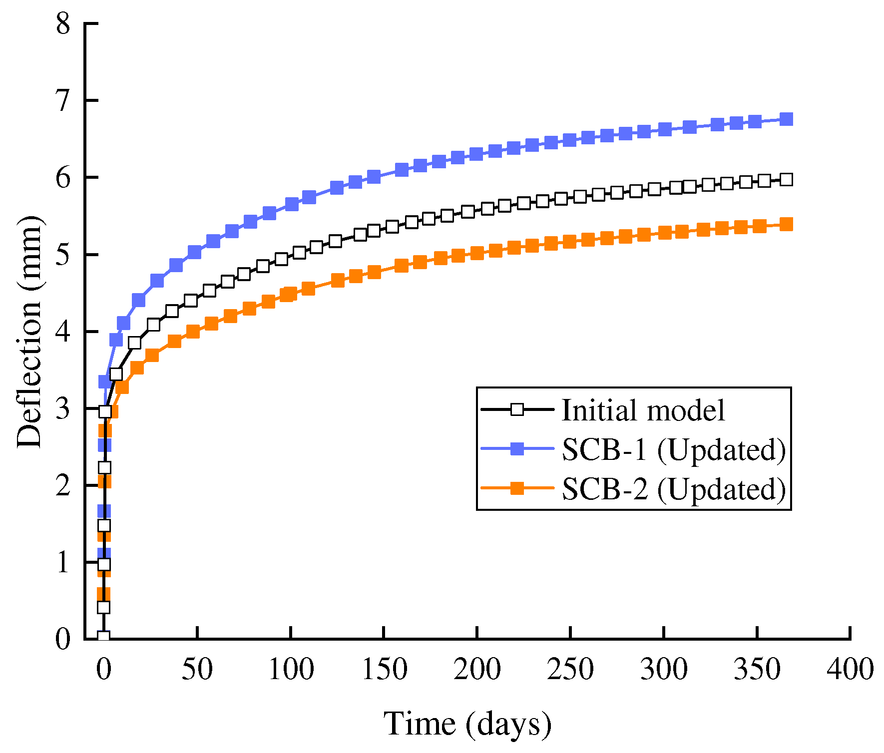
The evolution of deformation in SCBs under long-term loading is influenced by various factors, including the elastic modulus, the creep and shrinkage characteristics of the concrete, the elastic behavior of the steel beam, and the bond slip mechanism at the steel–concrete interface. Figure 16 illustrates the predicted long-term deflection curves before and after the model update, highlighting the distinct “three-stage characteristic” of the long-term deflection evolution: the initial loading stage, the mid-term stable growth stage, and the long-term asymptotic stability stage.

The comparison of the long-term deflection curves derived from the initial model and the updated model (SCB-1 and SCB-2) reveals that the updated model offers a more accurate depiction of the long-term deflection behavior of SCBs, particularly in the middle and later stages. The rapid deflection growth observed in the early phase of long-term loading reflects the prompt response of the SCBs during the initial deformation phase. This phenomenon is primarily attributed to the shrinkage and creep of the early concrete, as well as the elastic compression of the steel beams. Additionally, the hydration reaction and stress redistribution within the concrete may further contribute to the initial-stage deflection. Over time, the rate of deflection growth gradually decreases, transitioning into the mid-term steady growth stage. During this stage, the creep effect of the concrete becomes the dominant factor influencing deflection, while the bond–slip properties at the steel–concrete interface begin to play a more pronounced role. The updated model more accurately captures the deformation behavior of SCBs at the current stage, especially in the mid-to-late phase, and the predicted results are closer to the actual situation than those obtained before the update. Under prolonged loading, the deflection curve progressively flattens, indicating a significant deceleration in the deformation growth rate of the SCBs. Eventually, the deflection increment converges, signifying that the internal stress and deformation distribution within the structure have stabilized, and the system reached equilibrium.

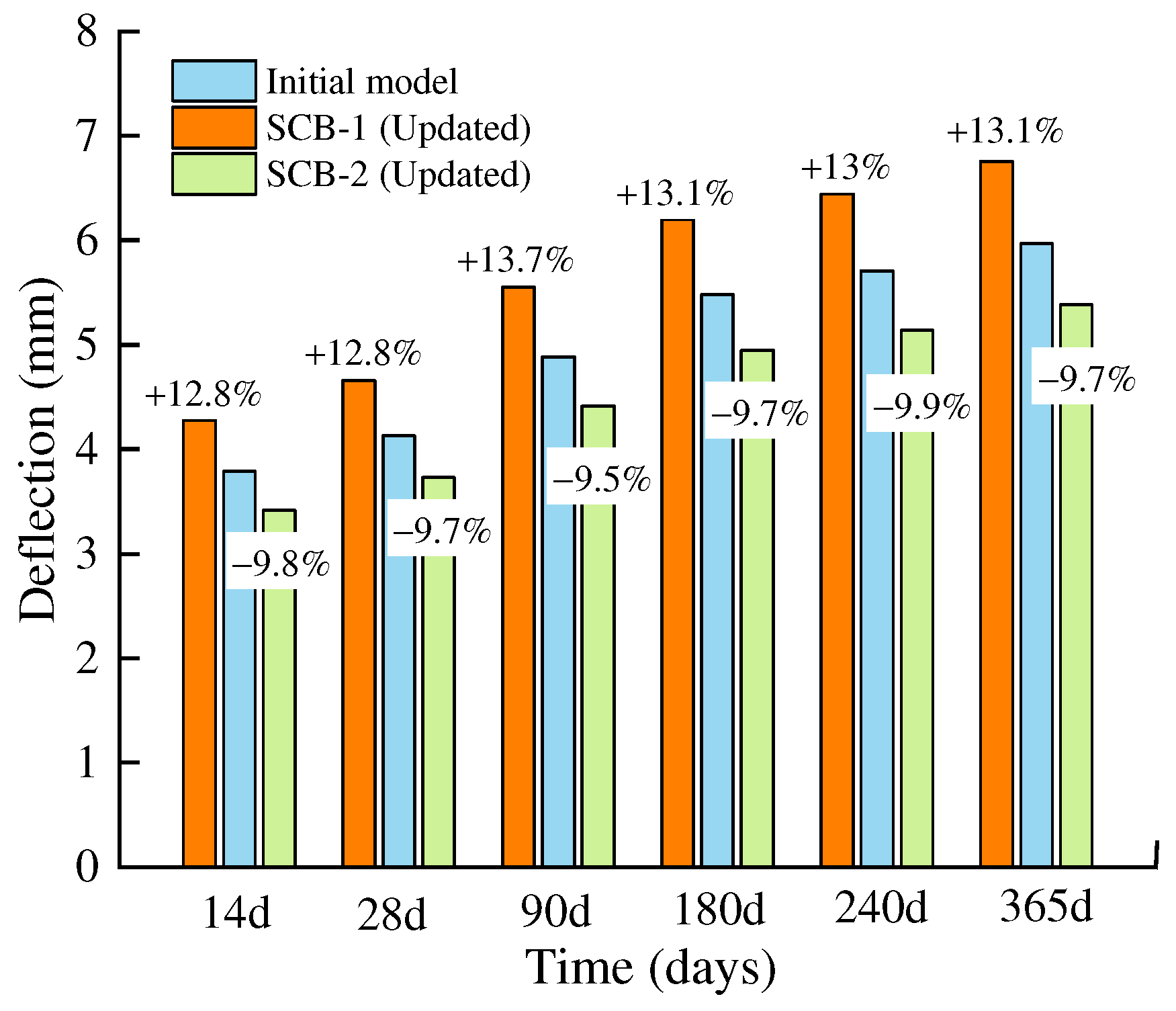
Figure 17 illustrates the deflection calculation results at various loading time points (14, 28, 90, 180, 240, and 365 days). From the figure, it is evident that the deflection calculations of the updated model exhibit significant optimization across all time points. Specifically, the deflection calculation results for SCB-1 improve by approximately 12.8% to 13.7% compared to the initial results at all time points. Conversely, the deflection calculation results for SCB-2 show a reduction of about 9.5% to 9.9%, highlighting the effectiveness of the model updates.

7. Conclusions

This study systematically examined the long-term deflection evolution of SCBs using a FEM dynamic updating method based on the Bayesian framework. The modal testing of two SCBs (SCB-1 and SCB-2), which shared identical parameters, revealed discrepancies between the initial FEM predictions and the actual structural performance in terms of frequencies and mode shapes. These findings underscore the significant influence of fabrication errors and material heterogeneity on the dynamic characteristics of structures. By utilizing measured data and applying the Bayesian approach, the key parameters of the FEM were updated. The updated model demonstrated an enhanced agreement between the calculated modal frequencies and mode shapes and the experimental results. Using the updated model, the long-term deflections of the SCBs were recalculated. The findings indicate that, after model updating, the long-term deflection of SCB-1 increased by 13.1%, while that of SCB-2 decreased by 9.8%. This discrepancy not only underscores the importance of model updating in accurately predicting the structural performance of complex composite foundations, especially in light of the uncertainties associated with local parameters, but also highlights the necessity for model adjustments in the long-term performance assessment of utilizing SCBs in practical bridge engineering.

The results of this study emphasize the necessity and effectiveness of FEMU methods based on experimental data, offering a more reliable framework for assessing and predicting the long-term performance of SCBs. This approach significantly mitigates risks associated with model uncertainties and enhances the safety and reliability of engineering structures. Future research will focus on the experimental validation of the model updating method in predicting the long-term performance of SCBs. Additionally, efforts will also be made to extend this approach to real bridge projects incorporating SCBs, in order to establish a foundation for assessing the long-term performance of actual bridges.