Study on the Wind Pressure Distribution in Complicated Spatial Structure Based on k-ε Turbulence Models

Abstract

Understanding wind pressure distribution on structures is crucial for evaluating design wind loads, especially for complex designs. This study investigated the wind pressure distribution on a windmill shape building with intricate geometries, i.e., the Chengdu Future Science and Technology City Exhibition Centre. Both wind tunnel test and CFD simulations are conducted to analyze the wind pressure distribution on building surface. Since the research object has intricate geometries, featuring sharp corners, curved surfaces, and ridges, the Reynolds Average Navier-Stokes (RANS) method adopting k-ε turbulence models is employed in the CFD simulations. Furthermore, scalable wall functions and non-structured grids with appropriate refinement on both turbulent regions and structural surfaces are also adopted in the RANS method. A comparison between the simulation results and wind tunnel tests demonstrated that the numerical simulations based on RANS method effectively capture surface wind pressure distribution on complex structures. This study reveals the occurrence of complicated flow phenomena that lead to a very complex wind pressure distribution on the surface of the structure, and drastic variance of the wind pressure coefficient is observed. Moreover, it is found that wind pressure distribution on the surface of the structure is highly sensitive to wind angle, exhibiting extreme negative pressure coefficients of −1.1, −1.0, and −1.8 at angles of 0°, 30°, and 60°, respectively. The analysis of the flow field around the structure at various wind angles reveals that its complex shape significantly alters the flow dynamics, creating distinct vortices and wake patterns at different angles. Consequently, CFD simulations help to understand wind loads on structures and improve wind resistance design.

1. Introduction

Complex spatial structures are the preferred structural form for public buildings such as exhibition halls and terminals. These structures are lightweight, highly flexible and wind sensitive. Due to the intricate body shape, they exhibit significant characteristic turbulence under wind loads, making them prone to complex flow phenomena such as flow separation and reattachment, resulting in a highly complicated distribution of wind pressure on the surface of the structure. Therefore, it is extremely difficult to determine the wind load for the design of such structures [1].

Theoretical analysis of wind pressure distribution on complex spatial structures is nearly impossible, leading to reliance on wind tunnel tests [2,3,4]. For instance, Uematsu et al. conducted experiments in turbulent boundary layers to develop a computer-assisted system for evaluating wind loads on spherical dome roofs [5]. Chen et al. characterized the wind pressure distribution on the cantilevered roof and evaluated the performance of various aerodynamic optimization devices through wind tunnel experiments [6]. Frontini et al. aimed to simplify and expedite the wind-resistant design of roof structures by computing the dynamic response of a stadium using data from wind tunnel tests to derive a small set of Multi-target Equivalent Static Wind Loads [7]. Rizzo et al. undertook wind tunnel experiments on a hyperbolic paraboloid structure with rectangular and square bases, discovering varying wind pressure distributions across different curvatures [8]. These studies highlight the complex characteristics of wind load distribution, which heavily depend on the intricate external shapes of structures. Therefore, it is essential to quantitatively investigate wind pressure distribution on complex structures. However, scaled models from wind tunnel tests often fail to accurately replicate local details of the prototype essential for generating complex flow patterns. Additionally, constraints within the wind tunnel’s working section can lead to discrepancies between test conditions and the true atmospheric boundary layer, resulting in experimental outcomes that may not fully reflect real-world scenarios. The long duration and high costs of these experiments hinder the collection of adequate data for reliably evaluating wind loads in structural design.

Accurate determination of design wind loads on complex structures can be achieved through effective numerical simulations that provide detailed wind pressure distributions. This approach mitigates the challenge of limited data for complex structures. With advancements in computing power, computational fluid dynamics (CFD) methods, particularly turbulence analysis using Reynolds Average (RANS), have become increasingly popular in structural wind engineering. Xin et al. analyzed the near-roof wind speed and friction velocity on gable roofs using the Realizable k-ε turbulence model, while Peren et al. applied the SST k-ω turbulence model to simulate the wind pressure distribution of a leeward sawtooth roof [9,10]. Studies show that the RANS simulation method effectively captures complex flow phenomena around structures and wind pressure distribution while visually representing the surrounding flow field. This contributes to understanding wind load formation mechanisms and aids in shape optimization. However, the turbulence model’s assumptions of isotropy and eddy viscosity result in inaccurate flow separation estimates on blunt bodies and overestimated turbulence energy generation on the windward side. As a result, the computational wind engineering community largely views these turbulence models as limited in accurately depicting the turbulence characteristics of building surfaces, and the varying outcomes of different models further undermine the credibility of numerical simulations [11,12].

The Large Eddy Simulation (LES) method separates turbulence into large and small-scale eddies, directly simulating the former with numerical techniques while parameterizing the latter with turbulence models. This approach may yield more accurate turbulence statistics and captures variations in turbulence scale and spatial distribution, making it particularly beneficial for complex wind field simulations. Consequently, LES is generally deemed more reliable than the RANS method, positioning it as the prevailing trend in computational wind engineering [13,14]. Li et al. employed the LES method to study wind effects on the 486 m-long roof of Shenzhen Citizens Centre [15]. Liu et al. examined wind loads on a uniquely shaped retractable gymnasium in Hangzhou, China, through a combination of wind tunnel tests and LES [16]. Although these cases highlight the effectiveness of LES, Blocken emphasized that it does not render the RANS method obsolete [17]. While LES is inherently superior, it involves greater simulation complexity and a much larger computational cost, and without best practice guidelines, it may yield less accurate and reliable results compared to RANS. Han et al. found that the computational costs of LES are about 20 times higher than RANS simulations, but LES often under-predicts results at the highest measurement levels compared to meteorological tower data in their study of atmospheric boundary layer flow over complex terrain [18]. RANS results show satisfactory accuracy across various practical applications. Researchers and engineers are leveraging increased computational power to perform RANS simulations on larger and more complex problems [17,19].

The RANS method is integral to engineering, effectively blending empirical formulations with turbulence models for accurate wind analysis of structures. It is anticipated to remain a key computational fluid dynamics tool in engineering research [20,21]. However, the accuracy of RANS results is heavily dependent on the chosen turbulence model and meshing, with the turbulence model being particularly crucial [22]. The k-ε model, the first practical two-equation model, is noted for its robustness, simplicity, and ease of implementation. While SST, LES, and other models are increasingly favored for highly anisotropic flows or high-precision applications [14,23], K-ε models remain essential for fully turbulent, high Reynolds number flows, and rapid engineering assessments. Liu et al. evaluated several eddy viscosity models, including Spalart-Allmaras (SA), standard k-ε, RNG k-ε, and Wilcox k-ω, finding that RNG k-ε performed best for high flow characteristics [24]. Quaresma et al. compared the standard k-ε, RNG k-ε, and standard k-ω RANS turbulence models in simulations of flow within a pool-type fishway with bottom orifices [25]. Pool Blanco et al. compared the applications of achievable k—ε and SST k—ω on the hyperbolic surface of mast supported tension structures [26]. It has been demonstrated that improved variants of k—ε models, such as Realizable and RNG, can consolidate their application value in specific complex structures through targeted modifications. By employing wall functions, it can effectively minimize mesh requirements in near-wall regions, making it popular in structural wind engineering. Yet, when using the k-ε model on complex structures, the mesh must meet wall function requirements related to y+ while accommodating geometric complexities. This alignment is vital for ensuring accuracy and computational efficiency in RANS simulations of wind pressure distribution. Therefore, it is essential to match the turbulence model with the proper wall function and meshing strategy to maintain the credibility and efficiency of RANS analysis results.

This paper examines the Chengdu Future Science and Technology City Exhibition Centre, a new landmark in eastern Chengdu. The building features a dynamic design with 18 curved surfaces that evoke a windmill, complemented by three large concave areas and various complex curvilinear forms. Its structure showcases significant curvature variations, sharp corners, and ridges, leading to irregular planes and elevations, as illustrated in Figure 1. To address this complexity, Rhino was employed for detailed geometric modeling, and a hybrid meshing strategy was developed to improve the efficiency of numerical methods through an effective combination of wall functions. To validate the RANS method and its various turbulence models for assessing wind pressure distribution on complex spatial structures, three models were selected: the Realizable k-ε, RNG k-ε, and Standard k-ε models. The average wind pressure coefficient and its surface distribution were analyzed, comparing results with a wind tunnel test using a 1:50 refined rigid manometric model. Additionally, the flow field around the structure was simulated to visually depict phenomena such as flow separation and reattachment, enhancing the understanding of wind load effects on the structure.

2. Wind Tunnel Test

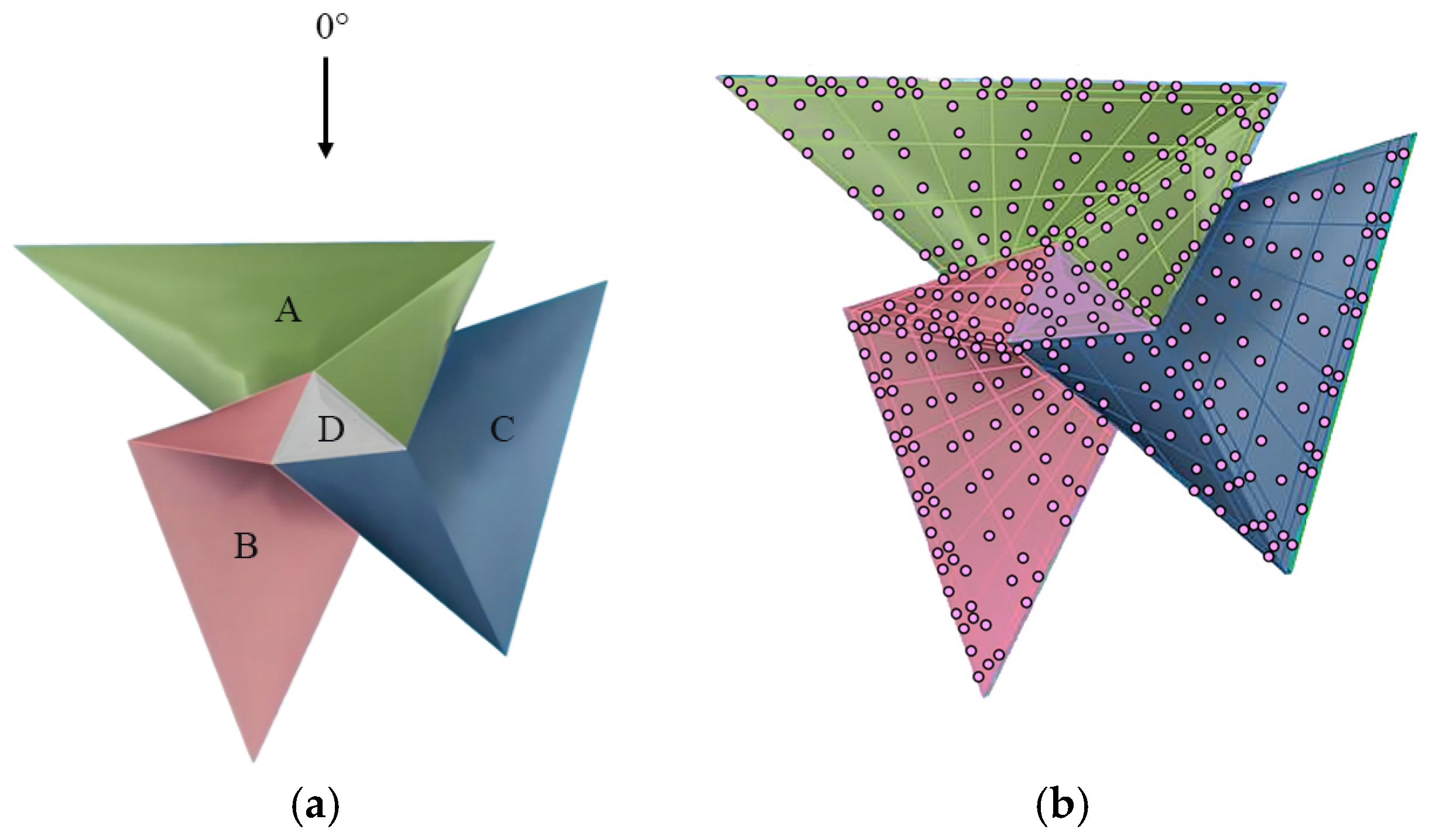
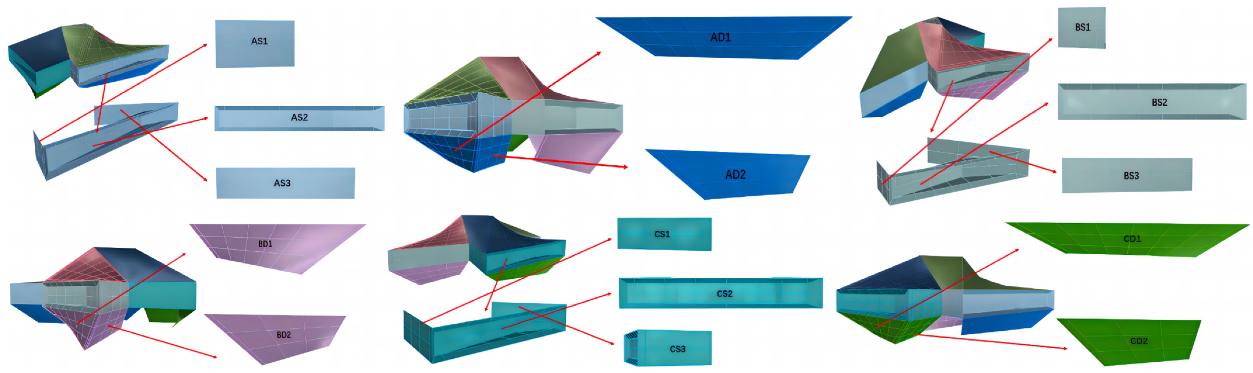
2.1. Test Model

The wind tunnel test for the Future Science and Technology City Exhibition Centre was performed in the XNJD-3 industrial wind tunnel at the Wind Engineering Test and Research Centre of Southwest Jiaotong University. The test section measures 36 m long, 22.5 m wide, and 4.5 m high. Figure 2 depicts the 1:50 scaled model used for the tests and taps distribution on the model surfaces, while Figure 3 illustrates the wind angles, with test conditions varying every 10° counterclockwise, resulting in a total of 36 conditions.

The structure consists of four main areas: A, B, C, and D, as illustrated in Figure 4. Each area is further divided into three height-based sub-regions: upper (AU), central (AS), and lower (AD) for zone A, containing 59, 28, and 36 subzones, respectively. Zones B and C follow the same division pattern, with AU, BU, and CU representing their roofs, while DD denotes the area enclosed by the ridge line.

Table 1. Detailed subdivision of the structure.

Structural Main Zones	Structural Subregions	Quantity of Subzones
A	AU	59
	AS	28
	AD	36
B	BU	59
	BS	28
	BD	36
C	CU	54
	CS	30
	CD	36
D	DD	7

details these zones, and Figure 4 shows the locations of the smaller zones. The pressure measurement system operates synchronously with a sensor range of 1000 Pa, a data acquisition time of 60 s, and a sampling frequency of 256 Hz. The vertical wind profiles of mean wind speed and turbulence intensity are shown in Figure 5. The reference wind speed is 7 m/s.

2.2. Wind Tunnel Test Results

The expression for the mean wind pressure coefficient is,

$$C_p={\displaystyle \raisebox{1ex}{$2(P_i-P_0)$}\!\left/ \!\raisebox{-1ex}{$\left({\rho }_a{v}_h^2\right)$}\right.}$$

(1)

where $P_i$ is the hydrostatic pressure on the surface of the structure; $P_0$ is the pressure at the reference point; ${\rho }_a$ is the density of air; $v_h$ is the top wind velocity unimpeded by the structure.

Figure 6 illustrates the average wind pressure coefficients for a typical area at a 0° wind direction during the wind tunnel test. Zone A, facing the wind, exhibits notable gradients in wind pressure coefficients across its upper, middle, and lower sections—AU, AS2, and AD1. Flow separation occurs at the leading edge of AU, where the wind pressure coefficient drops to −1.0 and rises to 0.0 upon reattachment at the rear. The windward sub-region AS2 exhibits a positive wind pressure coefficient that peaks in the middle to upper zone, whereas the lower windward sub-region AD2 has a smaller positive wind pressure coefficient due to its receding platform shape.

Zone C, located on the left side of the structure’s middle section, experiences both windward exposure and interference from zone A. This results in a complex wind pressure distribution in zone C, with a steeper gradient of wind pressure coefficients than in zone A. The sloping roof with multiple ridges in sub-region CU leads to negative wind pressure coefficients, with several instances reaching −1.0. In sub-region CS3, which is partially windward and partially obstructed, the wind pressure coefficient fluctuates from 0.8 to −0.4, characterized by dense contour lines and a complicated pattern. Although sub-region CD2 is windward, it is influenced by tail flow from zone A, resulting in a positive wind pressure coefficient with a complex distribution.

Zone B is centrally located at the rear of the structure and has a tapered shape. Consequently, the wind pressure coefficients and gradient fluctuations are minimal in sub-regions BU and BD2. Sub-region DD, which is relatively flat and surrounded by ridges, displays a negative wind pressure coefficient with negligible variation. Wind tunnel test results reveal that the wind pressure distribution of this complex structure, featuring multiple sharp corners, ridges, and curved surfaces, is extremely sensitive to its shape and location, resulting in distinct and intricate wind pressure patterns. Therefore, numerical simulation is crucial for a comprehensive understanding of the wind pressure distribution in this complex structure, providing clearer insights into wind loads.

3. Numerical Simulation in CFD

3.1. Determination of Turbulence Models and Treatment of Wall-Adherent Surfaces

The accuracy of numerical simulations using the RANS method heavily depends on the turbulence model chosen, making the selection of an appropriate model essential [11,27]. The SA (Spalart-Allmaras) model’s abrupt transition between laminar and turbulent flow produces a negative vortex viscosity, causing instability that high-precision solutions struggle to suppress, often leading to computational failure [28]. The k-ω model can introduce numerical instability and complicate wall distance calculations [29]. The average wind pressure on complex structures increases with the Reynolds number before stabilizing [30], indicating that high Reynolds number wind pressure distributions are more suitable for determining design wind loads. The k-ε series turbulence model is adept at predicting flow fields at high Reynolds numbers but requires suitable wall treatment for precision [31]. While the Standard k-ε model achieves sufficient convergence and accuracy in engineering calculations, it struggles with strongly separated flows and high curvature [32]. The RNG k-ε model effectively simulates complex flows like separation and secondary flows but is constrained by its assumption of isotropic vortex viscosity [33]. The Realizable k-ε model aligns Reynolds stress with actual turbulence and manages flow separation well; however, it can produce unphysical turbulence viscosity under certain conditions, affecting results [34]. To assess the performance of various k-ε models, this paper utilizes the RANS method with three turbulence models to predict the wind pressure distribution for the Chengdu Future Science and Technology City Exhibition Centre.

The turbulent kinetic energy and its dissipation rate transport equations for the Realizable k-ε model are,

$$\rho {\displaystyle \frac{Dk}{Dt}}={\displaystyle \frac{\partial }{\partial x_j}}\left[\right(\mu +{\displaystyle \frac{{\mu }_t}{{\sigma }_k}}\left){\displaystyle \frac{\partial k}{\partial x_j}}\right]+G_k+G_b-\rho \epsilon -Y_M$$

(2)

$$\rho {\displaystyle \frac{D\epsilon }{Dt}}={\displaystyle \frac{\partial }{\partial x_j}}\left[\right(\mu +{\displaystyle \frac{{\mu }_t}{{\sigma }_{\epsilon }}}\left){\displaystyle \frac{\partial \epsilon }{\partial x_j}}\right]+\rho C_{1}S\epsilon -\rho C_2{\displaystyle \frac{{\epsilon }^2}{k+\sqrt{\nu \epsilon }}}+C_{1\epsilon }{\displaystyle \frac{\epsilon }{k}}{C}_{3\epsilon }{G}_b$$

(3)

where $\rho$ is the fluid density; $t$ is time; $x_j$ is the coordinate component; $\mu$ is the kinematic viscosity; $\nu$ is the kinematic viscosity coefficient; ${\mu }_t$ is the vortex viscosity coefficient; $G_k$ and $G_b$ represent turbulent energy production from mean velocity gradients and buoyancy effects, respectively; $Y_M$ represents the contribution of pulsating compressible turbulence to the total dissipation rate; $C_1=\mathit{max}[0.43,{\displaystyle \frac{\eta }{\eta +5}}]$, $\eta =S{\displaystyle \frac{k}{\epsilon }}$, $S=\sqrt{2S_{ij}{S}_{ij}}$, $S_{ij}$ is the time-averaged strain rate tensor of the flow; $C_{1\epsilon }$,$C_{3\epsilon }$ and $C_2$ are constants; ${\sigma }_k$ and ${\sigma }_{\epsilon }$ are the turbulent Prandtl numbers for the turbulent kinetic energy and its dissipation rate, respectively.

The turbulent kinetic energy transport equations for the Standard k-ε, RNG k-ε, and Realizable k-ε models share a similar form but differ in their approaches for calculating turbulent viscosity, the turbulent Prandtl number for diffusion, and the relationship between generating terms $\rho C_{1}S\epsilon$ and $G_k$ in the dissipation rate in the transport equation.

The treatment of the near-wall region is crucial in turbulence modeling but often overlooked [35]. The high normal velocity gradient in the boundary layer, where turbulence generation, transport, and diffusion are most intense, necessitates a finer mesh to accurately capture these phenomena. Two primary methods for near-wall treatment are the direct solution of the viscous substrate and the wall function method. The direct method requires a dense mesh in viscous and transition regions to simulate near-wall turbulence effectively, leading to challenges like poor stability, low convergence efficiency, and high memory demands [36]. The wall function method avoids solving for the viscous bottom and buffer layers by linking wall quantities to variables in the turbulent core, addressing the entire domain. Accurate near-wall flow resolution can be achieved by strategically placing the first layer nodes near the wall during meshing. However, determining the wall function for complex shapes is challenging, as intricate flow phenomena may not conform to the simple logarithmic law, potentially impacting computational accuracy. Despite these challenges, the simplicity, cost-effectiveness, and ease of implementation of wall functions make them a popular choice for complex engineering problems.

To ensure accuracy and stability in the k-ε turbulence model simulation, this paper employs the Scalable Wall Function to extend the range of y+, allowing the generated mesh to meet wall function requirements. Figure 7 shows the location and y+ distribution in key areas. For improved numerical stability and high computational accuracy, the convective term is discretized using a quadratic windward format with third-order accuracy. The SIMPLEC algorithm is employed for velocity-pressure coupling, with residuals set to 10⁻⁴. Wind pressure on the windward face of the structure is monitored until stabilization, indicating convergence [37].

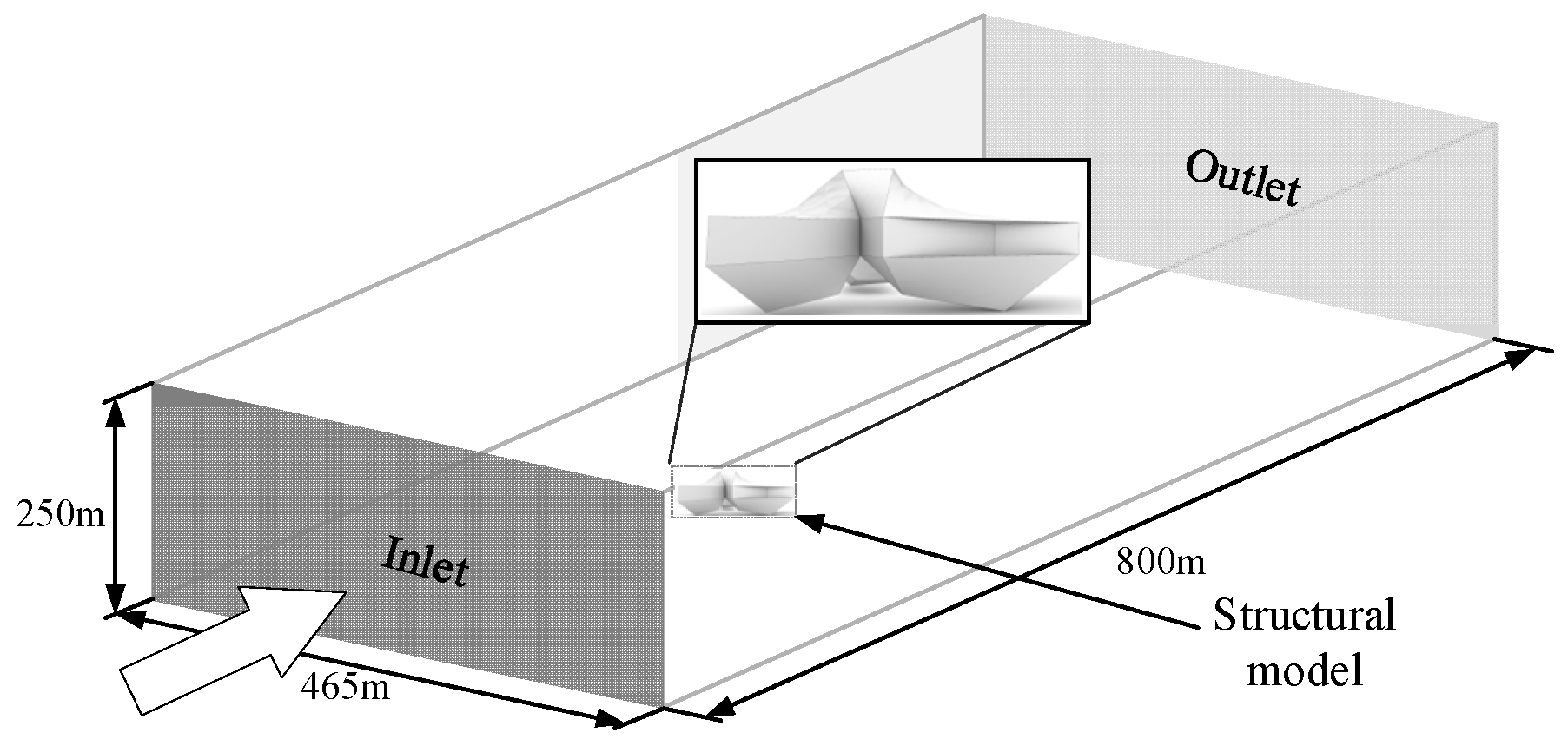
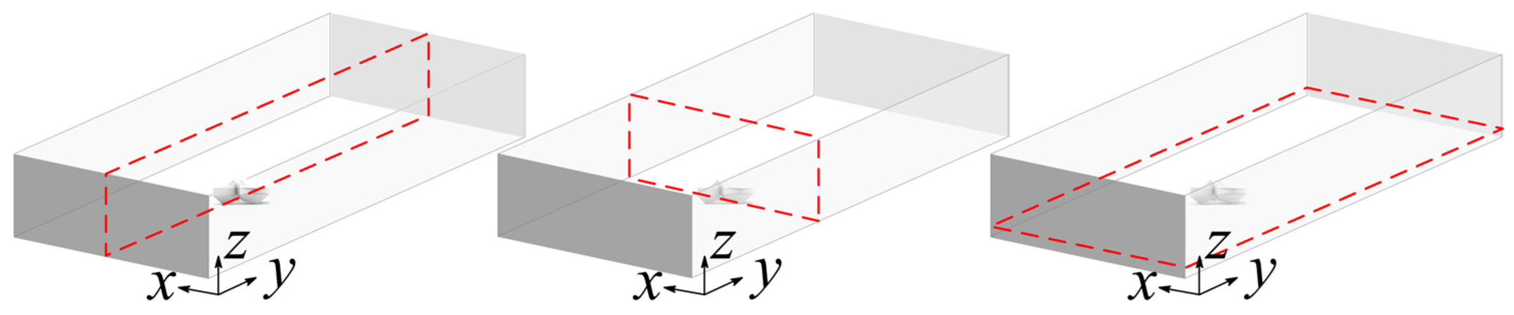
3.2. Computational Domain and Boundary Conditions

The Future Science and Technology City Exhibition Centre measures 65 m × 58 m × 25 m. Due to the complexity of the structure and the resulting large grid count for modeling, terrain was excluded. However, since terrain’s primary impact is on roughness and turbulence intensity, matching these parameters to wind tunnel test conditions when calculating wind pressure effectively accounts for the terrain’s influence. The computational domain is 800 m × 465 m × 250 m (Figure 8), with a blocking rate of 1.40%. The basic wind pressure at the building site is 0.35 KN/m² at a height of 10 metres as per China’s GB 50009-2012 Code for Structural Loading of Buildings [38]. Both the reference height and gradient height are maintained consistent between the wind tunnel testing and CFD simulations.

The inlet boundary condition employs a velocity inlet with a wind profile as,

$$v_z=v_{10}{\left({\displaystyle \frac{z_h}{z_{10}}}\right)}^{\alpha }$$

(4)

where $v_z$ and $v_{10}$ are the mean wind velocities at a height of $z_h$ above the ground and at a height of 10 m above the ground, respectively; roughness index $\alpha =0.15$.

The turbulent kinetic energy $k$ and dissipation rate $\epsilon$ of the incoming flow are,

$$k=1.5{\left(v_z{I}_z\right)}^2$$

(5)

$$\epsilon ={\displaystyle \raisebox{1ex}{${0.09}^{\frac{3}{4}}{k}^{\frac{3}{2}}$}\!\left/ \!\raisebox{-1ex}{$L$}\right.}$$

(6)

where $I_z$ and $L$ are the turbulence intensity and turbulence integral scale, respectively; $I_z=0.1\times {\left({\displaystyle \raisebox{1ex}{$z_h$}\!\left/ \!\raisebox{-1ex}{$300$}\right.}\right)}^{-\alpha -0.05}$, $L=100\times {\left({\displaystyle \raisebox{1ex}{$z_h$}\!\left/ \!\raisebox{-1ex}{$30$}\right.}\right)}^{0.5}$ [39].

A fully developed outflow boundary condition is applied at the outlet, ensuring a zero normal gradient for all flow quantities. A no-slip wall condition is enforced for the ground and building surfaces, while a free-slip wall condition is used for the sides and top of the computational domain.

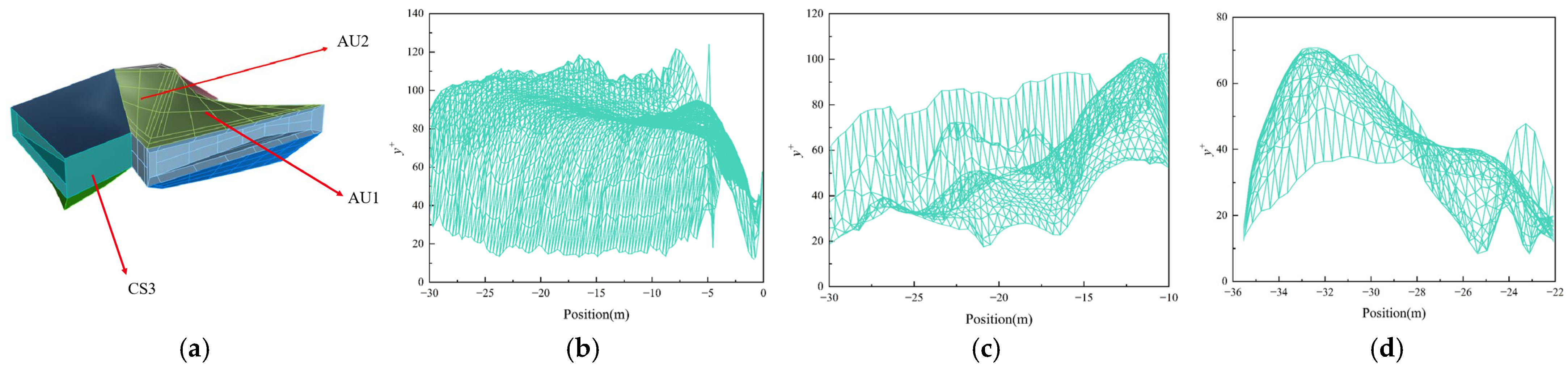
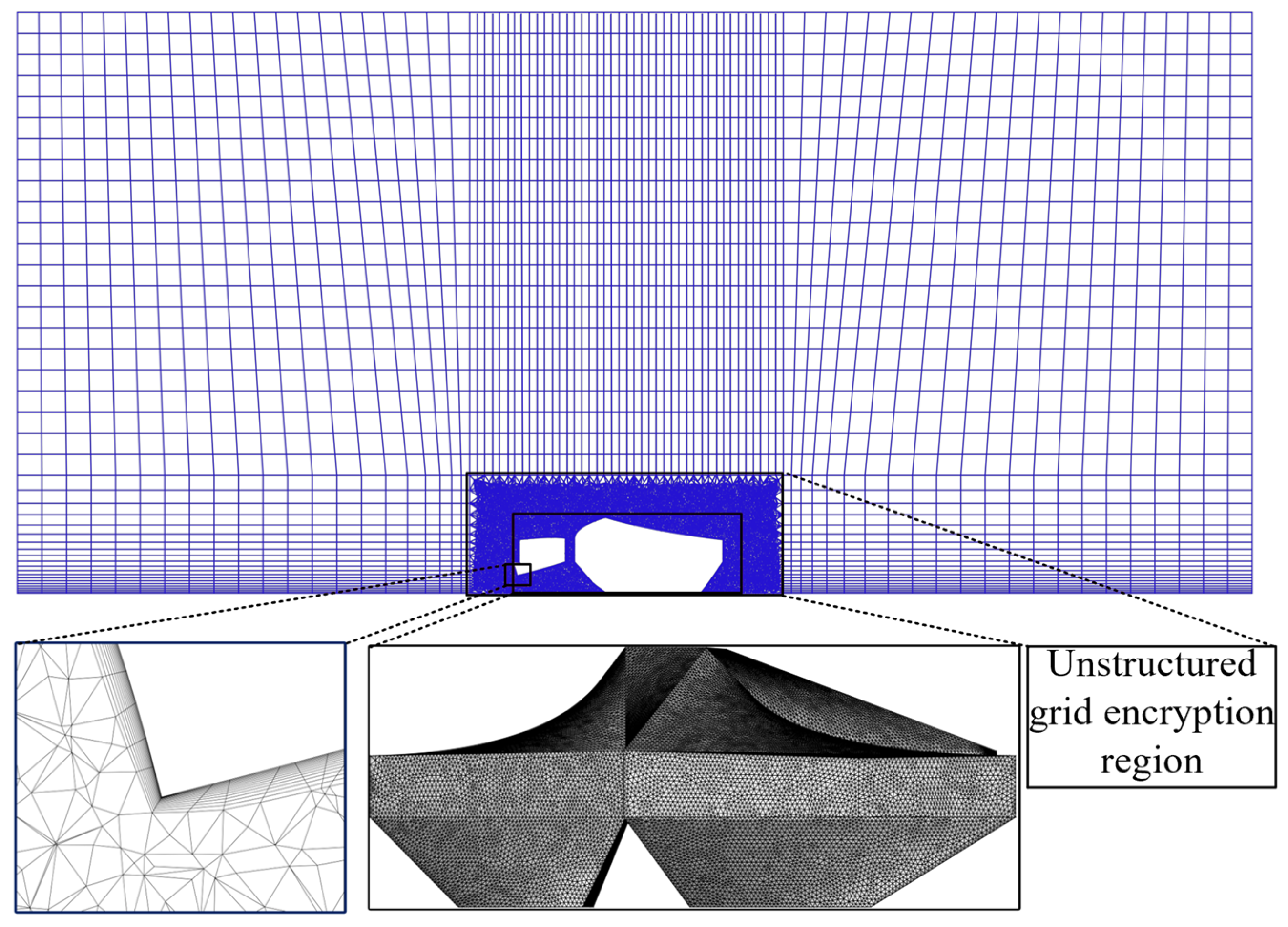
3.3. Mesh Partition

Mesh quality, resolution, and convergence significantly affect CFD calculation results. Structured meshes provide regular connections leading to high accuracy, stability, and efficiency, but struggle with complex geometries. Conversely, unstructured grids allow for easier generation and adaptability to intricate shapes but are less controllable and often require more nodes, which can reduce computational efficiency [40,41]. This study proposed a hybrid approach that combines structured and unstructured grids to mitigate the effects of mesh variations on computational outcomes. Due to the structure’s complexity, a structured mesh proved unsuitable to apply in turbulent areas near the building; therefore, an unstructured mesh was employed. While structured grids were utilized further away. Mesh refinement prioritized sharp corners and ridges of the structure, improving the capture of complex flow phenomena across its surface. The mesh size in the flow field and the boundary layer near the wall is vital for accuracy. Consequently, the rectangular area of 85 m × 85 m × 30 m, as depicted in Figure 9, features a refined mesh with variable first-layer heights on the structural surface.

To enhance computational efficiency and ensure the reliability and accuracy of results, grid independence is verified by using four grid parameters M1, M2, M3 and M4 listed in

Table 2. The grid parameters.

Meshing Scheme	M1	M2	M3	M4
Size of surface grid/m	1	0.8	0.5	0.3
Size of unstructured grid/m	2	1.5	1	0.8
Height of the first layer of the grid m	0.005	0.005	0.003	0.003
Number of mesh cell	1,121,514	1,896,425	3,002,519	5,804,584

. M3 exemplifies the hybrid meshing strategy with a global mesh size of 4 m, while the non-structural grid size is refined to 1 m. The first layer of the near-wall grid has a height of 0.003 m and a growth rate of 1.15, comprising 15 boundary layer grid layers. The dimensionless distance y+ ranges from 30 to 160, meeting the scalable wall function requirement with a body mesh count of 3,002,519.

To evaluate the impact of grid resolution on simulation accuracy, Figure 10 compares the mean wind pressure coefficients at points in zones A, B, C, and D derived from the Realizable k-ε model using different meshing strategies with wind tunnel test results. Additionally,

Table 3. Average relative deviation of different zones under different meshing schemes.

Meshing Scheme	M1	M2	M3	M4
A	47.95%	38.02%	25.06%	27.03%
B	30.99%	25.01%	16.96%	13.06%
C	34.07%	37.97%	28.96%	25.06%
D	25.93%	31.91%	23.03%	17.98%

quantifies the average relative deviation of mean wind pressure coefficients obtained from the Realizable k-ε model at a 0° wind angle for varying grid sizes. The mean wind pressure coefficients for zones A, B, and C using grid M1 show significant relative deviations, particularly in zone A, which approaches 50%. This indicates that M1’s low resolution fails to adequately capture the complex turbulence in that area. Although M2 improves upon M1, deviations in zones A and C remain around 40%. In contrast, grids M3 and M4 reduce these deviations to below 30%, reflecting a marked improvement in accuracy. Despite M4 having nearly double the grid count of M3, the accuracy increase is minimal, particularly in zone A, where M3 outperforms M4. Thus, for balancing computational accuracy and efficiency, M3 grids are chosen for all subsequent analyses.

4. Analysis of the Calculation Results

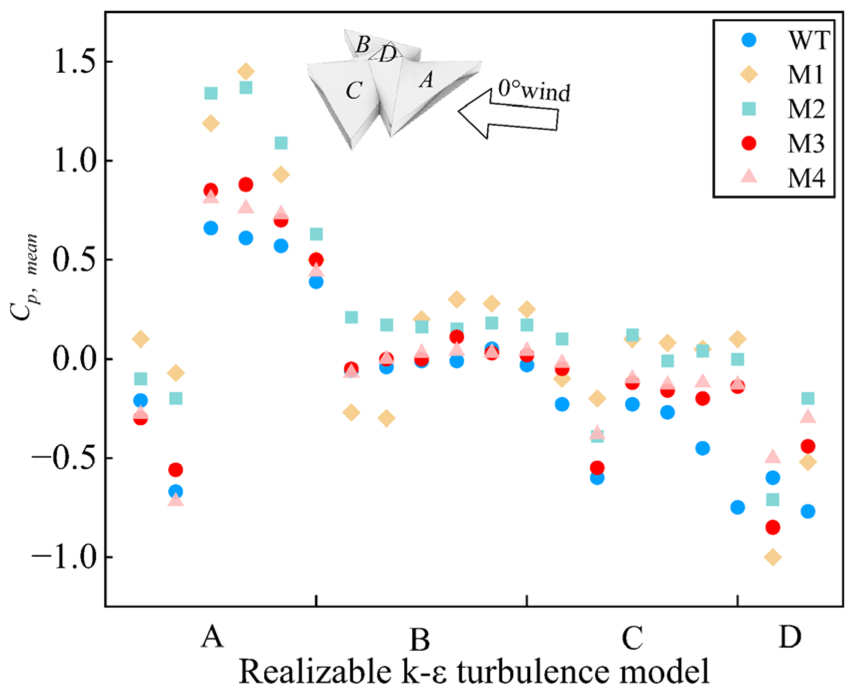
4.1. Comparison of Various Turbulence Models

Figure 11 presents the mean wind pressure coefficient distributions for the structure at a 0° wind angle, analyzed using the RANS method with the Realizable k-ε(TM1), RNG k-ε(TM2), and Standard k-ε(TM3) models.

Simulated wind pressure distributions from three k-ε turbulence models differ numerically from wind tunnel tests but display a similar overall trend. The models yield slightly higher positive wind pressure distributions and extreme coefficients due to their enhanced simulation of high turbulence. However, theoretical limitations in diffusion modeling result in an overestimated turbulence integration scale, leading to higher computed values than experimental observations. Conversely, the negative wind pressure distributions and extreme negative coefficient amplitudes from the turbulence model are generally slightly lower than those from wind tunnel tests, with a few exceptions. This discrepancy arises from poor diffusion performance and the assumption of isotropic vortex viscosity coefficients. These limitations restrict the models’ accuracy in simulating complex turbulence phenomena such as transitions, adverse pressure gradients, and flow separations, leading to weaker separation and earlier reattachment points. Although the Realizable k-ε model better captures Reynolds stress and aligns more closely with wind tunnel results, it still struggles with dissipation rate diffusion. Additionally, complex geometries with sharp corners, curved surfaces, and ridges complicate flow separation and reattachment, exacerbating these modeling shortcomings and leading to significant simulation errors.

Figure 12 shows the minimum and maximum mean wind pressure coefficients from three turbulence models along with wind tunnel test results (WT). In sub-regions AU, BU, CU, and DD, corresponding to the structural roof area, the k-ε turbulence models closely match the wind tunnel data, indicating an accurate simulation of the roof area’s wind characteristics.

Satisfactory simulation results are achieved in sub-regions AS and BS, while sub-region CS exhibits the opposite. This discrepancy arises because sub-region AS, on the windward side, is mainly influenced by incoming wind turbulence. Sub-region BS, in the wake area, exhibits slow turbulence changes, allowing the k-ε turbulence model to effectively predict flow characteristics. Conversely, sub-region CS, situated at the sides of the structure, experiences airflow separation from the windward side and strong flow separation at the sharp corner of sub-region AS. These factors create complex vortex interactions in sub-region CS that challenge the k-ε models and lead to substantial prediction errors.

The AD, BD, and CD sub-regions at the bottom of the structure are influenced by downward shear airflow. However, their bottom faces are designed as receding platforms to mitigate this effect. Sub-region AD significantly shades sub-region BD, resulting in a small and slowly changing wind pressure coefficient there. The turbulence model effectively simulates the winding characteristics of sub-region BD, yielding results that closely match wind tunnel tests. The wind pressure distribution in the positive pressure areas of sub-regions AD and CD mainly stems from the turbulence of the incoming wind, leading to higher prediction accuracy. While the retreat of the bottom zones weakens flow separation at the edges, negative pressure zones still develop. However, the k-ε models struggle to capture the complex turbulence in these separation zones, causing some errors in predicting the negative pressure distributions in sub-regions AD and CD.

While the Realizable k-ε model offers marginally more accurate simulation results than the Standard and RNG k-ε models across most regions, it requires significantly longer computation times (357 h) compared to the RNG (231 h) and Standard (186 h) k-ε models for simulating the wind pressure distribution on the structure.

Table 4. Extreme mean wind pressure coefficients: wind tunnel vs. numerical simulation results and their deviations.

Subregions	WT	TM1		TM2		TM3
	Extreme Value	Extreme Value	Deviation	Extreme Value	Deviation	Extreme Value	Deviation
AU	−1.33	−1.10	17.3%	−1.00	24.8%	−0.90	32.3%
BU	−0.34	−0.40	17.6%	−0.25	26.5%	−0.20	41.2%
CU	−1.10	−0.79	28.2%	−0.53	51.8%	−0.45	59.1%
DD	−1.10	−1.19	8.2%	−1.14	3.6%	−1.00	9.1%
AS2	0.82	0.91	10.9%	1.10	34.1%	1.00	22.0%
CS3	0.72	0.92	27.8%	1.01	40.3%	1.00	38.9%
AD1	0.57	0.81	42.1%	0.87	52.6%	0.84	47.4%
BD2	0.21	0.32	52.4%	0.11	47.1%	0.08	61.9%
CD2	0.66	0.83	25.8%	0.85	28.8%	0.83	25.8%

lists the extreme mean wind pressure coefficients for each region from wind tunnel tests and the k-ε turbulence models.

Figure 11 and Figure 12 and Table 4 reveal that the most severe negative wind pressure coefficient from the wind tunnel tests in region A is −1.33, found at the lower left tip of sub-region AU. After flow separates on the left side of sub-region AU, it is blocked by sub-region CU, leading to vortices and a significant negative pressure zone. In comparison, the Realizable k-ε turbulence model predicts a minimum coefficient of −1.10 at the ridge of sub-region AU, while wind tunnel tests report −1.00 at the same spot. This ridge, formed by a gently curved surface, experiences flow separation. The Realizable k-ε turbulence model effectively simulates the single flow around the structure. However, it falls short in capturing the complex phenomena of strong separation at the sharp corner of sub-region AU and the obstruction in sub-region CU, resulting in inaccurate predictions of high negative pressure in the left cusp of sub-region AU. Meanwhile, the maximum positive wind pressure coefficients in region A, measured from wind tunnel tests and the k-ε model, are both found in the center of sub-region AS2, with values of 0.82 and 0.91, respectively; these positions and values are closely aligned. This sub-region’s large concave shape significantly hinders incoming wind, creating a zone of high positive pressure. The k-ε model effectively predicts this turbulence-dominated flow region.

The most unfavorable negative wind pressure coefficients in region B, derived from wind tunnel tests and the Realizable k-ε turbulence model, are found near the intersection of sub-region BU and sub-region DD at the ridge line, with values of −0.34 and −0.40, respectively. The incoming flow separates at this ridge line, having already separated at the gable end and ridge line of sub-region AU. As the wind pressure recovers upon attachment, a secondary separation occurs at sub-region BU’s ridge, resulting in a relatively lower absolute value for the most unfavorable negative wind pressure coefficient in region B. Conversely, the maximum positive wind pressure coefficients for both the wind tunnel tests and simulations in region B are observed on the right side of sub-region BD2, measuring 0.21 and 0.32, respectively. This area, located near the back edge of the leeward side, experiences a gradual change in wind pressure coefficients due to shielding from regions A and C. In region C, the most unfavorable negative wind pressure coefficients from both the wind tunnel test and the Realizable k-ε model are located near the ridge of sub-region CU, yielding values of −1.10 and −0.79, respectively. The maximum positive wind pressure coefficients in region C are at the middle of sub-region CD2, at 0.66 and 0.83, respectively. Notably, the maximum positive pressure coefficients for regions B and C are situated near the leeward side of the structure, with sub-region CD2 exhibiting a higher positive wind pressure coefficient. This is due to the sharp corner of region B being closer to the structure’s trailing edge, resulting in a distinctly posterior cusp shape and a weak flow separation at the sharp corner, which creates a gradual wind pressure coefficient gradient. In region DD, characterized by ridges, the most unfavorable negative wind pressure coefficients recorded from wind tunnel tests and Realizable k-ε turbulence model simulations are −1.10 and −1.19, respectively. Overall, the wind pressure distributions in zones B, C, and D are accurately predicted based on the Realizable k-ε models.

The analysis indicates that wind pressure distributions from the k-ε turbulence models align closely with wind tunnel test results. However, these models struggle to accurately predict complex flow phenomena caused by the drastic changes in structural shape, stemming from inherent theoretical limitations. While the Realizable k-ε model has been improved to better align Reynolds stress with actual flow conditions, fundamental flaws persist, limiting its ability to predict complex flow fields. Furthermore, significant deviations at specific points between wind tunnel test results and numerical simulations may be attributed to the model’s neglect of terrain features, which critically influence localized wind behavior. While the simulations match wind profile and turbulence intensity parameters from the test, the exclusion of terrain effects likely alters the localized aerodynamic interactions, ultimately impacting the peak values of pressure coefficients. Generally, the k-ε series turbulence model with a scalable wall function and coordinated meshing strategy achieves satisfactory results, except for significant flow field deviations in certain regions due to overly complex structures.

4.2. Wind Pressure Distribution at the Structure Surface

The study analyzed wind pressure distributions at 0°,30°, and 60° angles from the Realizable k-ε turbulence model to evaluate the impact of different wind angles on surface pressure, as shown in Figure 13.

At a 0° wind angle, sub-region AS2 is perpendicular to the incoming flow, while most of CS3 faces the wind despite a small obstruction from AS2. This configuration creates a large windward surface, producing a significant positive pressure area in AS2 with a maximum wind pressure coefficient of 0.91. Flow separation at AS2’s sharp left corner creates vortices that CS3 interrupts, causing steep changes in surface wind pressure, evident from closely packed contour lines. The wind pressure coefficient decreases sharply from 0.92 to −0.21. Some airflow also separates at the windward eaves, creating a negative pressure zone with a worst-case coefficient of −0.60. As the flow reattaches, the wind pressure recovers, gradually raising the coefficient to 0.30. At the ridge, strong flow separation results in considerable negative pressure areas on either side, reaching a minimum coefficient of −1.10. A secondary reattachment downstream restores the wind pressure, increasing the coefficient to 0.20. Finally, as flow approaches the wake zone, separation occurs at BU’s sharp corner. BU’s inward shape diminishes the wake zone and weakens entrainment, resulting in a low wind pressure coefficient at its rear with minimal variation.

At a 30° wind angle, the incoming flow strikes sub-region AS2 obliquely, generating a peak wind pressure coefficient of 0.9 on the right side, despite the area’s small size. The coefficient diminishes from right to left with sparse contours. In sub-region AD2, the coefficient also peaks at 0.7 on the right side, exhibiting similarly sparse contours. As the flow moves rearward, separation occurs on both sides of AS2 and region AU. The separated flow on the left impacts sub-region CS3, creating a positive pressure area with a peak of 0.6—lower than the 0.9 seen at a 0° angle due to the relationship between CS3 and the incoming flow. After crossing the roof ridge, the flow causes separation in sub-region CU, resulting in a negative wind pressure coefficient of -1.0, which quickly rebounds to −0.3, marked by dense contours and a steep gradient. Sub-region AU also experiences significant fluctuations in the wind pressure coefficient, particularly at the roof ridge where the upper sub-regions converge.

At a 60° wind angle, the edge of sub-region AS3 aligns with the incoming flow, making AS2, AS3, BS1, and BS2 windward. Sub-region BS1, nearly facing the wind, experiences the highest positive wind pressure coefficient of 1.10. Flow separation at the cornice of BS1 leads to vortex shedding and a rapid decline in the wind pressure coefficient from 1.10 to 0.40. The steep slope in the right part of sub-region AU yields a positive wind pressure coefficient peaking at 0.80. At the ridge of sub-region BU, strong flow separation creates a significant negative pressure zone on both sides, with the most unfavorable negative wind pressure coefficient of −1.80, approximately 1.6 times greater than the lowest coefficient for a 0° wind angle. Downstream of the ridge, secondary reattachment occurs, recovering wind pressure and increasing the coefficient to 0.20, characterized by a steep gradient and dense contours. At the rear of sub-region CU, the inward shape reduces both the wind pressure coefficient and its gradient near the wake zone, with values ranging from 0.10 to 0.20.

The analysis indicates that the surface wind pressure distribution of the complex body structure significantly varies with wind angles, emphasizing the importance of wind angle in this regard. The asymmetrical, windmill-like shape, featuring sharp corners and ridges, causes flow separation in various areas, leading to predominantly negative pressure on the surface and steep pressure gradients near separation points. This intricate wind pressure distribution is heavily influenced by the structure’s shape. At a 0° wind angle, the lowest negative wind pressure coefficient is −1.10 due to the roof’s gradual changes at the windward edge. At 30°, the distribution becomes more uniform, with a minimum negative pressure coefficient of −1.0, influenced by the angle between the windward sub-region and incoming flow, which slightly alters airflow. At 60°, interactions between wind and the edges of the windmill blades create a complex flow field with conical vortices, resulting in a negative wind pressure coefficient of −1.80 and a notable pressure gradient. Consequently, comprehensive assessment of wind safety at structural discontinuities is essential for specific wind angles.

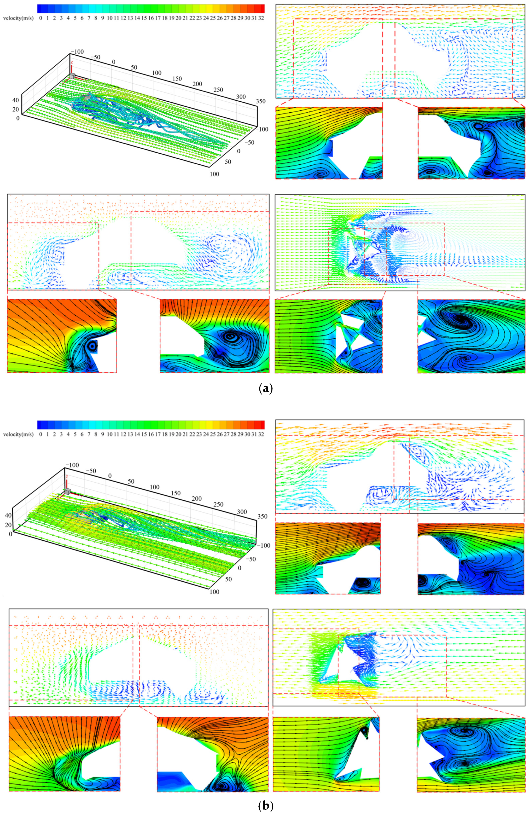
4.3. Airflow Field Around Structure

The flow field around the building often exhibits complex turbulent eddies, particularly due to its intricate structure with sharp corners and ridges. CFD simulations provide valuable insights into the wind load mechanisms and characteristics of these structures. This paper analyzes the wind field around the Future Science and Technology City Exhibition Centre at wind angles of 0°,30°, and 60°, using the Realizable k-ε turbulence model. It focuses on the wind speed vectors in the yz, xz, and xy planes, as illustrated in Figure 14.

Figure 15 illustrates wind speed streamlines and vector plots at wind angles of 0°, 30°, and 60°, displaying three-dimensional streamlines around the structure and wind speed vectors in the yz, xz, and xy planes, with this format continued in subsequent figures.

At a 0° wind angle, wind speed remains high until it encounters the structure, where it rapidly decreases due to obstruction. The wind speed vector plot in the yz-plane reveals flow separation at the sharp edges and gables of the windward surface, creating varying-sized vortices at the front, center, and rear of the structure. In the xz-plane, the vector plot indicates significant flow obstruction, causing a rapid drop in speed and vortex formation at multiple locations. The xy-plane vector diagram indicates that the structure’s inwardly closing sides lead to airflow separation and smaller vortices on both sides. The sharp corners of the BU and CU sub-regions at the rear create two larger vortices, but the overall inward structure shape leads to a quicker narrowing of the wake zone and an elongated wake.

At a 30° wind angle, the three-dimensional flow pattern around the structure reveals notable wind speed variations due to obstruction. The yz-plane wind speed vector plot indicates that the flow diverges upon hitting the structure, with some air moving upward and some downward over the ridge. The sharper forward corners relative to the 0° wind direction cause increased flow separation and a small cavity formation on the top surface of sub-region AU, which quickly reattaches. On the downwind side, larger vortices with lower wind speeds are generated, along with multiple shedding vortices trailing the structure. The xz-plane wind speed vector plots reveal distinct vortices only on the downwind side, with no significant shedding upwind. The xy-plane wind speed vector plots display two larger vortices at the rear, with the one aligned with the incoming wind being significantly larger, causing the wake area to shift towards it and narrow more slowly than in the 0° wind direction.

At a 60° wind angle, the three-dimensional flow diagram indicates that the incoming flow diverges on both sides of sub-region AU upon reaching the structure, leading to a gradual decrease in wind speed due to the alignment of the flow with the sideline of sub-region AS3 and the sharp corner of AU at the front.The wind speed vector plot in the yz-plane reveals a section of upward-accelerating flow, but after flow separation at the ridge, the velocity decelerates gradually without significant vortex formation. In the xz-plane, the flow around a 60° wind angle appears complex, characterized by numerous small vortices near the tops of the AU and BU sub-regions. The xy-plane wind velocity vector plot reveals three vortices of different sizes at the structure’s rear, with two larger vortices behind sub-region CU, resulting in a broad and elongated wake area.

The streamlines and wind speed vectors at various angles demonstrate how the structure alters the flow field, affecting both streamline patterns and flow speed. The flow around the complex structure varies significantly with different wind angles, highlighting the structure’s substantial impact on the flow dynamics and generating notable turbulence. Therefore, when designing for wind resistance, it is crucial to account for the interaction between the structure and the flow field, along with the influence of different wind angles.

5. Conclusions

This paper examines the Chengdu Future Science and Technology City exhibition center, where wind tunnel tests and CFD simulations assess mean wind pressure distribution and flow characteristics around the structure, leading to the following conclusions:

(1)

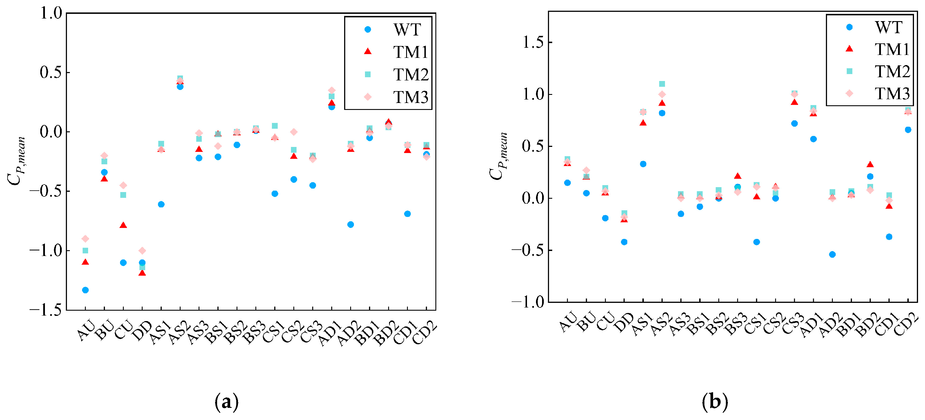
The wind pressure distribution of complex spatial structures is analyzed using RANS method with k-ε turbulence models, a scalable wall function, and a hybrid meshing strategy. Compared to wind tunnel tests, the RANS method slightly overestimates the positive wind pressure distribution range and the extreme positive mean wind pressure coefficient due to inherent limitations of the k-ε models, while underestimating the negative wind pressure distribution range and the absolute value of the extreme mean negative wind pressure coefficient. Although some flow prediction discrepancies occur at specific locations due to structural complexity, the RANS method effectively captures the overall flow characteristics of intricate structures and aligns closely with the distribution patterns in wind tunnel tests, demonstrating its suitability for such analyses.

(2)

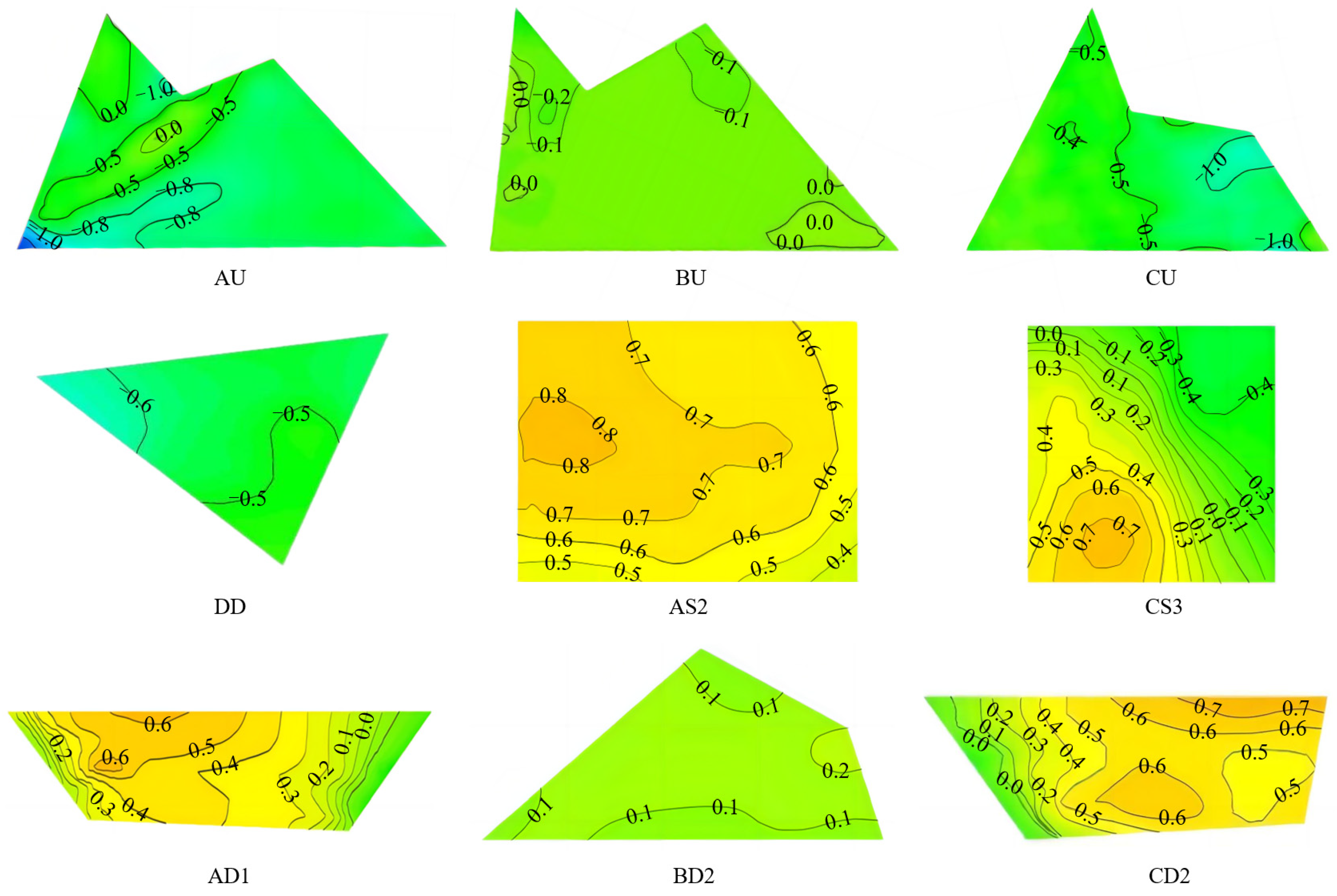
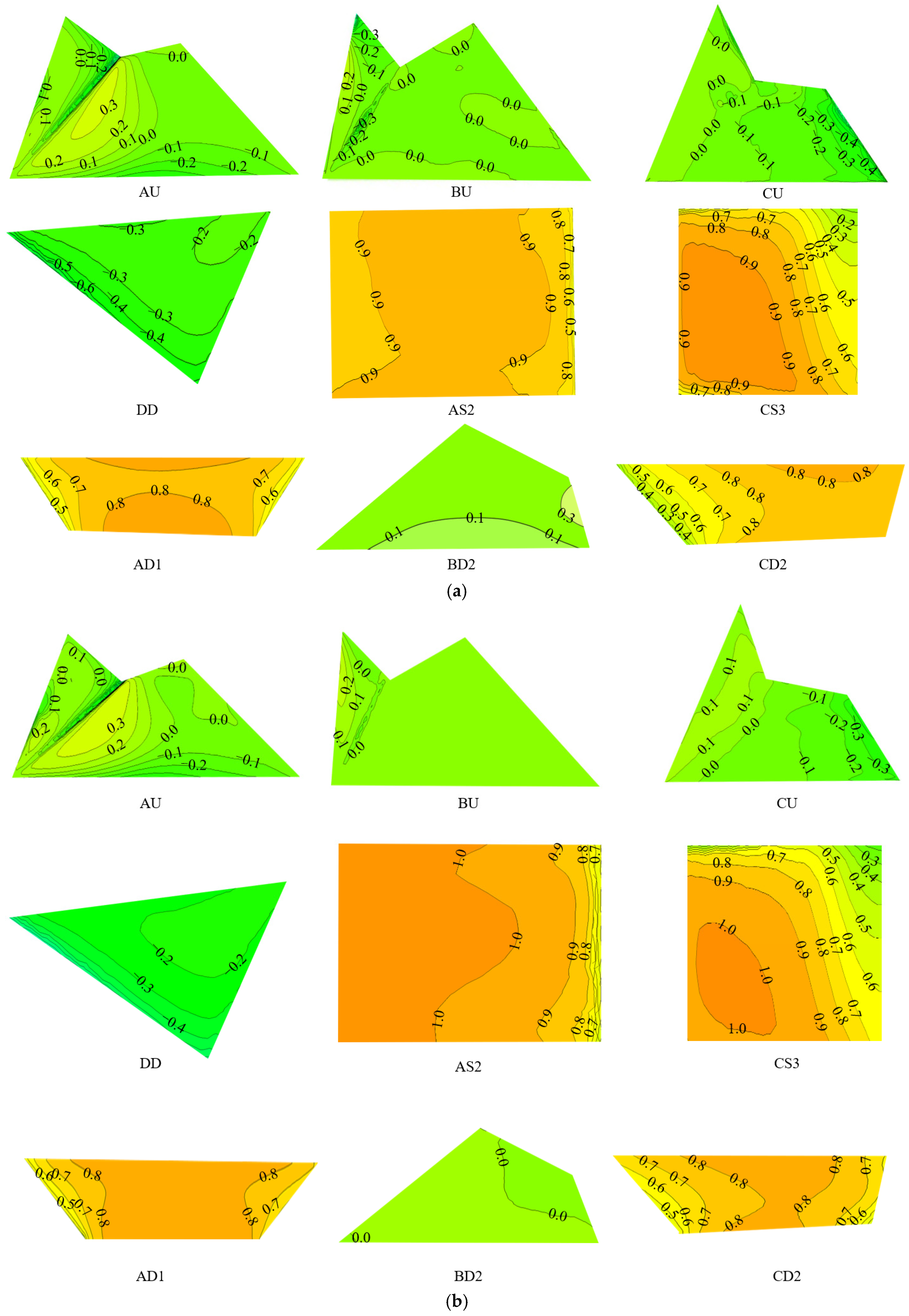
Simulation results using the RANS method with k-ε turbulence models are affected by the shape of complex structures in wind pressure distribution analysis. Accuracy is highest in smooth, flat areas, especially in the middle and lower sections. However, it decreases in regions with pronounced surface changes, such as large curved roofs, where complexity increases. Significant errors in mean wind pressure coefficients can occur at sharp corners due to insufficient modeling of complex flow separation.

(3)

The sharp corners, curved surfaces, ridges, and large internal concave features of the complex structure cause multiple flow separations at the edges and re-attachments on the roof. This results in a larger negative pressure zone and a steeper gradient of the unfavorable wind pressure coefficient. The leading edge blocks incoming flow, creating maximum positive pressures on the windward side, despite a minimal change in the pressure coefficient’s gradient. Additionally, the inward shape of the rear generates positive pressures on the lower part of the leeward side. Consequently, the intricate design creates a highly complex wind pressure distribution.

(4)

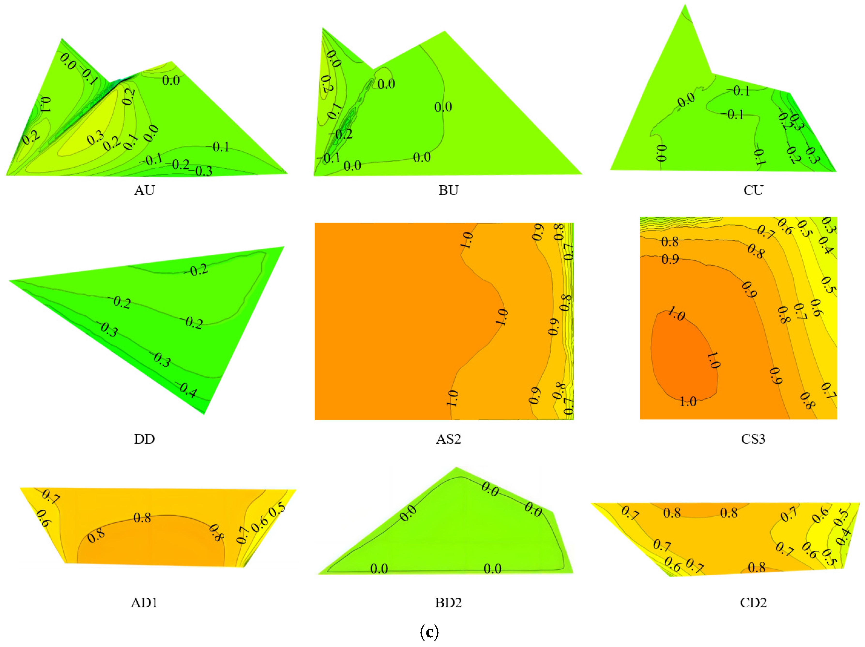
Wind pressure distribution on complex structures varies significantly with wind angles. Sharp corners and ridges cause flow separation at multiple points. Analysis shows the most severe negative wind pressure coefficients of −1.10 at 0° and −1.80 at 60°, with the latter being about 1.6 times greater. Furthermore, at 60°, the wind pressure coefficient contours are denser and the change gradient is steeper. Thus, wind pressure distribution is highly sensitive to wind direction for complex-shaped structures.

(5)

The numerical simulation method illustrates how the flow field around complex structures varies with different wind angles, highlighting the bypassing phenomenon. Flow separation occurs at gables, sharp corners, and ridges on the windward side, resulting in vortex shedding and multiple reattachments that create significant turbulence. As the wind angle changes, the wake flow adopts distinct forms, leading to considerable alterations in the surrounding flow field due to the structure’s intricate spatial profiles.

References

- Tian, Y.J.; Guan, H.W.; Shao, S.; Yang, Q.S. Provisions and Comparison of Chinese Wind Load Standard for Roof Components and Cladding. Structures 2021, 33, 2587–2598. [Google Scholar] [CrossRef]
- Shen, G.H.; Que, L.H.; Wan, H.P. Experimental Study on the Aerodynamic Characteristics of Combined Angle Transmission Tower Subject to Skew Wind. Adv. Struct. Eng. 2024, 27, 1016–1030. [Google Scholar] [CrossRef]
- Bandi, E.K.; Tamura, Y.; Yoshida, A.; Chul Kim, Y.; Yang, Q. Experimental Investigation on Aerodynamic Characteristics of Various Triangular-section High-rise Buildings. J. Wind Eng. Ind. Aerod. 2013, 122, 60–68. [Google Scholar] [CrossRef]
- Gu, M.; Wang, X.R.; Quan, Y. Wind Tunnel Test Study on Effects of Chamfered Corners on the Aerodynamic Characteristics of 2D Rectangular Prisms. J. Wind Eng. Ind. Aerod. 2020, 204, 104305. [Google Scholar] [CrossRef]
- Uematsu, Y.; Tsuruishi, R. Wind Load Evaluation System for the Design of Roof Cladding of Spherical Domes. J. Wind Eng. Ind. Aerod. 2008, 96, 2054–2066. [Google Scholar] [CrossRef]
- Chen, F.B.; Wang, W.J.; Zhou, J.F.; Shou, Z.R.; Li, Q.S. Experimental Investigation of Wind Pressure Characteristics and Aerodynamic Optimization of a Large-span Cantilevered Roof. Structures 2021, 34, 303–313. [Google Scholar] [CrossRef]
- Frontini, G.; Argentini, T.; Rosa, L.; Rocchi, D. Advances in the Application of the Principal Static Wind Loads:A large-span Roof Case. Eng. Struct. 2022, 262, 114314. [Google Scholar] [CrossRef]
- Rizzo, F.; D’asdia, P.; Ricciardelli, F.; Bartoli, G. Characterization of Pressure Coefficients on Hyperbolic Paraboloid Roofs. J. Wind Eng. Ind. Aerod. 2012, 102, 61–71. [Google Scholar] [CrossRef]
- Xin, L.G.; Zhou, X.Y.; Gu, M. Wind Tunnel Test and CFD Simulation of the Near-roof Wind Speed and Friction Velocity on Gable Roofs. J. Wind Eng. Ind. Aerod. 2022, 225, 105009. [Google Scholar] [CrossRef]
- Peren, J.I.; Van Hooff, T.; Ramponi, R.; Blocken, B.; Leite, B.C.C. Impact of Roof Geometry of an Isolated Leeward Sawtooth Roof Building on Cross-ventilation: Straight, Concave, Hybrid or Convex? J. Wind Eng. Ind. Aerod. 2015, 145, 102–114. [Google Scholar] [CrossRef]
- Durbin, P.A. Some Recent Developments in Turbulence Closure Modeling. Annu. Rev. Fluid Mech. 2015, 50, 77–103. [Google Scholar] [CrossRef]
- Slotnick, J.; Khodadoust, A.; Alonso, J.; Darmofal, D.; Gropp, W.; Lurie, E.; Mavriplis, D. CFD Vision 2030 Study: A Path to Revolutionary Computational Aerosciences. NASA Rep. 2014, NASA/CR-2014-218178. [Google Scholar]
- Rajasekarababu, K.B.; Vinayagamurthy, G.; Ajay Kumar, T.M.; Selvirajan, S. Experimental and Computational Investigation of Wind Flow Field on a Span Roof Structure. Int. J. High-Rise Build. 2022, 11, 287–300. [Google Scholar]
- Yang, Q.S.; Chen, F.X.; Tamura, Y.; Li, T.; Yan, B.W. Fluid-structure Interaction Behaviors of Tension Membrane Roofs by Fully-coupled Numerical Simulation. J. Wind Eng. Ind. Aerod. 2024, 244, 1056092. [Google Scholar] [CrossRef]
- Li, C.; Li, Q.S.; Huang, S.H.; Fu, J.Y.; Xiao, Y.Q. Large Eddy Simulation of Wind Loads on a Long-span Spatial Lattice Roof. Wind Struct. 2010, 13, 57–83. [Google Scholar] [CrossRef]
- Liu, M.; Li, Q.S.; Huang, S.H.; Shi, F.; Chen, F.B. Evaluation of Wind Effects on a Large Span Retractable Roof Stadium by Wind Tunnel Experiment and Numerical Simulation. J. Wind Eng. Ind. Aerod. 2018, 179, 39–57. [Google Scholar] [CrossRef]
- Blocken, B. LES over RANS in Building Simulation for Outdoor and Indoor Applications: A Foregone Conclusion? Build. Simul. 2018, 11, 821–870. [Google Scholar] [CrossRef]
- Han, Y.; Stoellinger, M.K.; Peng, H.W.; Zhang, L.H.; Liu, W. Large Eddy Simulation of Atmospheric Boundary Layer Flow over Complex Terrain in Comparison with RANS Simulation and On-site Measurements under Neutral Stability Condition. J. Renew. Sustain. Ener. 2023, 15, 023301. [Google Scholar] [CrossRef]
- Hanjalic, K. Will RANS Survive LES? A View of Perspectives. J. Fluid. Eng. Asme 2005, 127, 831–839. [Google Scholar] [CrossRef]
- Cecora, R.; Radespiel, R.; Eisfeld, B.; Probst, A. Differential Reynolds-stress Modeling for Aeronautics. AIAA J. 2015, 53, 739–755. [Google Scholar] [CrossRef]
- Peralta, C.; Navarro, J.; Cruz, I.; Toja-Silva, F.; Lopez-Garcia, O. Roof Region Dependent Wind Potential Assessment with Different RANS Turbulence Models. J. Wind Eng. Ind. Aerod. 2015, 142, 258–271. [Google Scholar]
- Potsis, T.; Tominaga, Y.; Stathopoulos, T. Computational Wind Engineering: 30 Years of Research Progress in Building Structures and Environment. J. Wind Eng. Ind. Aerod. 2023, 234, 105346. [Google Scholar] [CrossRef]
- Yang, Q.; Chen, F.; Yan, B.; Li, T.; Yan, J. A Transport Model of Convective Flow on Self-excited Vibrating Flat Flexible Roofs Using LES. J. Wind. Eng. Ind. Aerod. J. Int. Assoc. Wind. Eng. 2023, 238, 105426. [Google Scholar] [CrossRef]
- Liu, J.N.; Wang, D.X.; Huang, X.Q. Investigation of Turbulence Models for Aerodynamic Analysis of a High-pressure-ratio Centrifugal Compressor. Phys. Fluids. 2023, 35, 21. [Google Scholar] [CrossRef]
- Quaresma, A.L.; Romão, F.; Pinheiro, A.N. A Comparative Assessment of Reynolds Averaged Navier–Stokes and Large-Eddy Simulation Models: Choosing the Best for Pool-Type Fishway Flow Simulations. Water 2025, 17, 686. [Google Scholar] [CrossRef]
- Pool Blanco, S.J.; Hincz, K. Computational Wind Engineering of a Mast-supported Tensile Structure. Period. Polytech. Civ. Eng. 2022, 66, 210–219. [Google Scholar] [CrossRef]
- Rumsey, C.L. Apparent Transition Behavior of Widely-used Turbulence Models. Int. J. Heat Fluid Flow 2007, 28, 1460–1471. [Google Scholar] [CrossRef]
- Zhou, C.; Wang, Z.J. CPR High-order Discretization of the RANS Equations with the SA Model. In Proceedings of the 53rd AIAA Aerospace Sciences Meeting, Kissimmee, FL, USA, 5–9 January 2015; AIAA: Reston, VI, USA, 2015. [Google Scholar]
- Schoenawa, S.; Hartmann, R. Discontinuous Galerkin discretization of the Reynolds-averaged Navier-Stokes equations with the shear-stress transport model. J. Comput. Phys. 2014, 262, 194–216. [Google Scholar] [CrossRef]
- Karvelis, A.C.; Dimas, A.A.; Gantes, C.J. Unsteady Numerical Simulation of Two-dimensional Airflow over a Square Cross-section at High Reynolds Numbers as a Reduced Model of Wind Actions on Buildings. Buildings 2024, 14, 561. [Google Scholar] [CrossRef]
- Wilcox, D.C. Turbulence Modeling for CFD; DCW Industries: La Canada, CA, USA, 1993. [Google Scholar]
- Launder, B.E.; Spalding, D.B. Lectures in Mathematical Model of Turbulence; Academic Press: Cambridge, MA, USA, 1974; Volume 3, pp. 269–289. [Google Scholar]
- Yakhot, V.; Orszag, S.A. Renormalization Group Analysis of Turbulence I. Basic Theory. J. Sci. Comput. 1986, 1, 3–51. [Google Scholar] [CrossRef]
- Shih, T.H.; Liou, W.W.; Shabbir, A.; Yang, Z.G.; Zhu, J. A New k-ε Eddy Viscosity Model for High Reynolds Number Turbulent Flows. Comput. Fluids 1995, 24, 227–238. [Google Scholar] [CrossRef]
- Murakami, S. Overview of Turbulence Models Applied in CWE-1997. J. Wind Eng. Ind. Aerod. 1998, 74–76, 1–24. [Google Scholar] [CrossRef]
- Tominaga, Y.; Mochida, A.; Yoshie, R.; Kataoka, H.; Nozu, T.; Yoshikawa, M.; Shirasawa, T. AIJ Guidelines for Practical Applications of CFD to Pedestrian Wind Environment around Buildings. J. Wind Eng. Ind. Aerod. 2008, 96, 1749–1761. [Google Scholar] [CrossRef]
- Mani, M.; Dorgan, A.J. A Perspective on the State of Aerospace Computational Fluid Dynamics Technology. Annu. Rev. Fluid Mech. 2023, 55, 431–457. [Google Scholar] [CrossRef]
- GB 50009-2012; Load Code for the Design of Building Structures. Ministry of Housing and Urban-Rural Development: Beijing, China, 2012.
- AIJRLB-2004; AIJ Recommendations for Loads on Buildings. Architectural Institute of Japan: Tokyo, Japan, 2004.
- Baum, J.D.; Loehner, R.; Luo, H. High-Reynolds Number Viscous Flow Computations Using an Unstructured-grid Method. J. Aircr. 2005, 42, 483–492. [Google Scholar]
- Mohotti, D.; Wijesooriya, K.; Dias-da-Costa, D. Comparison of Reynolds Averaging Navier-Stokes (RANS) Turbulent Models in Predicting Wind Pressure on Tall Buildings. J. Build. Eng. 2019, 21, 1–17. [Google Scholar] [CrossRef]