Dynamic Performance Assessment and Model Updating of Cable-Stayed Poyang Lake Second Bridge Based on Structural Health Monitoring Data

Abstract

Structural health monitoring (SHM) systems are very useful for evaluating the performance of bridges in service. In this paper, the SHM system implemented on the Poyang Lake Second Bridge is investigated, and the monitored data are analyzed for performance evaluation, damage identification, and model updating of the bridge. First, the measured data are examined for environmental effects, structural behaviour, and modal identification. Based on the bridge construction information, a finite element (FE) model is constructed for the cable-stayed bridge. Subsequently, the regularized model updating approach is employed to calibrate the constructed numerical model by using the measured modal data. Several vibration-based methods for structural damage identification are proposed to inversely identify the simulated damage within the cable-stayed bridge using the test data. The results indicate that the measured structural responses, such as cable forces and bridge deck deflections, vary over time and highlight discrepancies in the initial FE model. This FE numerical model can then be effectively adjusted using the proposed model updating method, which enhances the connection between the real cable-stayed bridge and the modified FE numerical model. From the modal data, the simulated damage in the main structural members of the cable-stayed bridge can be correctly identified using the proposed methods.

1. Introduction

With the development of transportation infrastructure in China, cable-stayed bridges have become a major structural type for long-span bridges crossing rivers and roads [1]. Compared with traditional continuous beam bridges, the cable-stayed bridge is greatly reduced in size and the number of piers owing to the elastic supports offered by the cables, and its spanning capacity is then improved significantly. In comparison with suspension bridges, cable-stayed bridges exhibit better wind-resistance stability due to their greater lateral stiffness. Additionally, they do not require massive cable anchors. However, the performance of the cable-stayed bridge in service needs further investigation to ensure its safe operation over its lifetime. Dynamic characteristics are a fundamental consideration for the safe operation of long-span cable-stayed bridges, but these characteristics are susceptible to degradation over time in service [2]. Therefore, an SHM system is necessary to monitor the performance of the structure for safe operation [3,4].

The SHM system typically consists of many functional sub-systems, including the sensory system, data process system, condition evaluation system and safety warning system [5]. Advanced sensors such as fibre-optic sensors have been utilized for monitoring critical physical parameters of bridges, and sensors have been deployed at optimum positions on the structures [6,7]. The SHM data, such as accelerations, deflections and strains, can then be utilized for structure behaviour evaluation, dynamic performance analysis, operational modal analysis, dynamic model modification and damage detection [4,8,9,10]. From the operational modal analysis, modal properties including natural frequencies and mode shapes can be obtained from the measured acceleration data by various system identification methods, such as wavelet transform algorithms [11,12] and stochastic subspace identification methods [13,14,15,16]. The identified dynamic properties of the bridge can then be utilized for updating the associated FE model and for identifying structural damage. Furthermore, the structural performance of the bridges can be assessed and predicted by using continuously monitored data through the SHM system.

Despite the advancements in SHM systems, challenges remain in accurately representing the physical and geometric properties of actual bridges through FE models. FE models are typically constructed based on design and construction information. However, they often fail to fully capture the structural stiffness and boundary conditions of the constructed structures, which may not be appropriately modelled [17,18]. Consequently, this discrepancy may lead to differences in structural dynamic responses and modal parameters between numerical results and test data. In order to solve this problem, many structural model updating methods have been developed, including sensitivity analysis methods [19], the dynamic perturbation method [20] and the Bayesian numerical model updating method [21,22]. However, the process of updating models for complex structures, such as the cable-stayed Poyang Lake Second Bridge, remains a significant challenge, especially when only limited modal test data are available.

For an existing large cable-stayed bridge, various types of structural damage may occur in the bridge during its lifetime [3]. The damage may be caused by natural phenomena like earthquakes and environmental corrosion or human factors such as improper structural maintenance and collisions from vehicles and ships. If damage to the structure cannot be detected in time and treated properly, it can not only affect the normal operation of the bridge but also, in some extreme cases, even cause catastrophic accidents such as sudden failure or collapse [23]. Vibration-based structural damage identification techniques provide a useful approach for monitoring vibration under ambient excitation and detecting structural damage [24]. Recent studies have explored dynamic analysis and damage detection in cable-stayed bridges [25,26,27,28,29], demonstrating the effectiveness of vibration-based methods in identifying structural damage [30,31,32,33,34]. The principle underlying these methods is that structural damage modifies parameters like stiffness, which can alter the dynamic properties of the bridge. Cheng et al. proposed a two-stage damage detection framework that integrates fractal theory and FE model updating using acceleration data [35]. Comanducci et al. investigated damage detection approaches through statistical analysis and showed notable effectiveness in mitigating the influence of environmental factors and in extracting features that are highly sensitive to damage [36]. With the advancement of computational capabilities and sensing technologies, researchers have started to explore damage identification methods based on artificial intelligence algorithms [37,38]. However, these methods have only been successful in laboratory models and simple structures. Structural damage identification and damage identification for large-scale, complex civil engineering structures, such as the Poyang Lake Second Bridge, are still challenging, and further investigations are required.

In this paper, the SHM system of the Poyang Lake Second Bridge is investigated, and the monitored data are utilized for various engineering analyses, including structural performance evaluation, dynamic model updating and damage identification. First, the measured data from the SHM system are employed for structural performance assessment, and the modal data of the bridge are extracted from acceleration measurements through operational modal analysis. Then, the identified modal data are utilized for updating the full-scale 3D FE numerical model by using the regularized updating method, improving the connection between the observed data and numerical estimates. Finally, from the calibrated numerical model, various damage scenarios are simulated on the cable-stayed bridge, and inverse identification of the simulated damage is performed through the utilization of vibration-based methods for damage identification. The results demonstrate that the full-scale FE model can be effectively calibrated, and damage to the cable-stayed bridge can be accurately identified from the modal data.

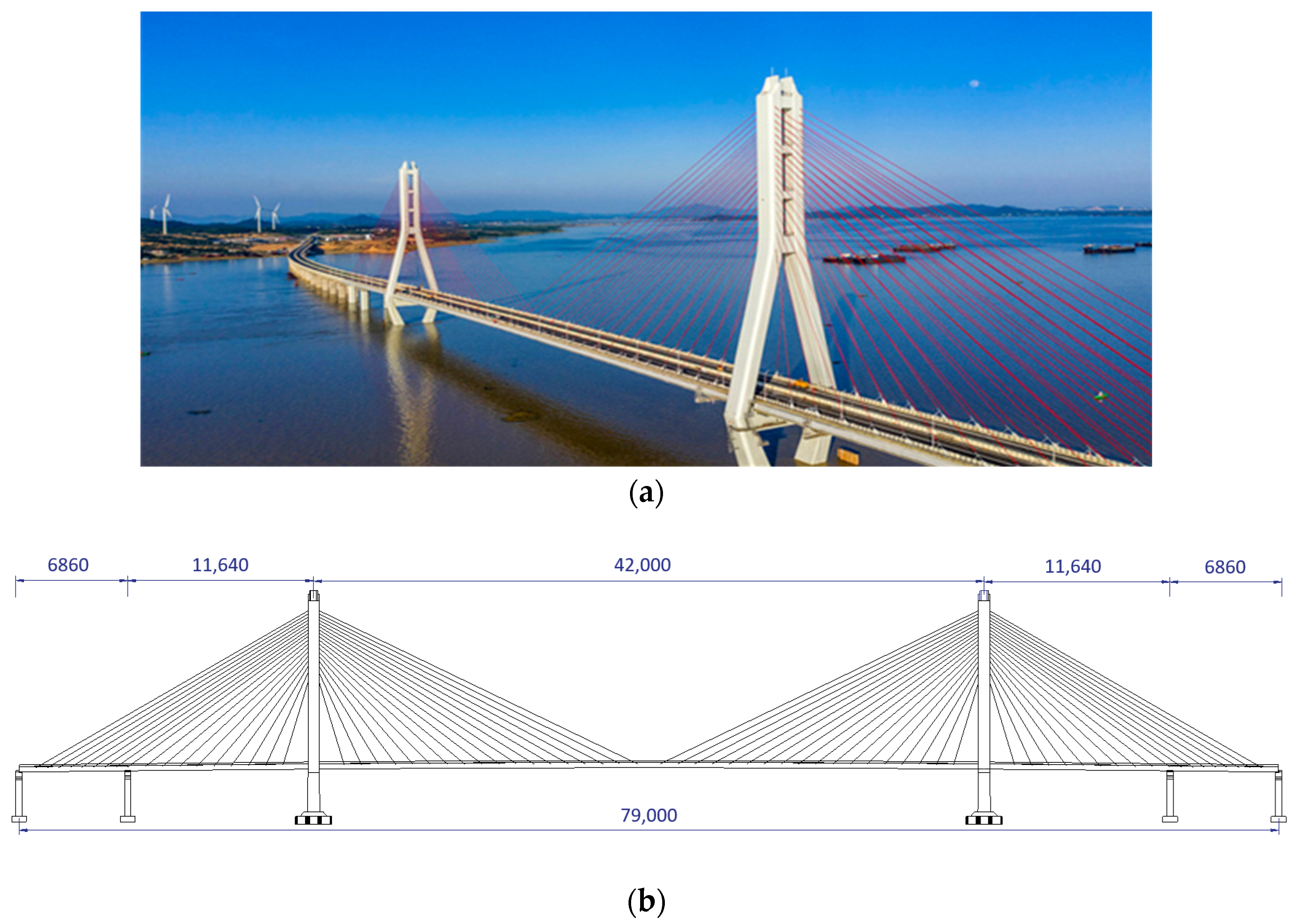
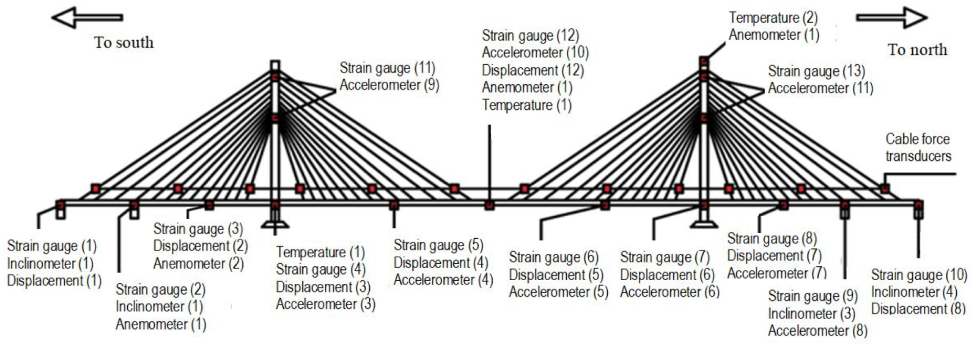
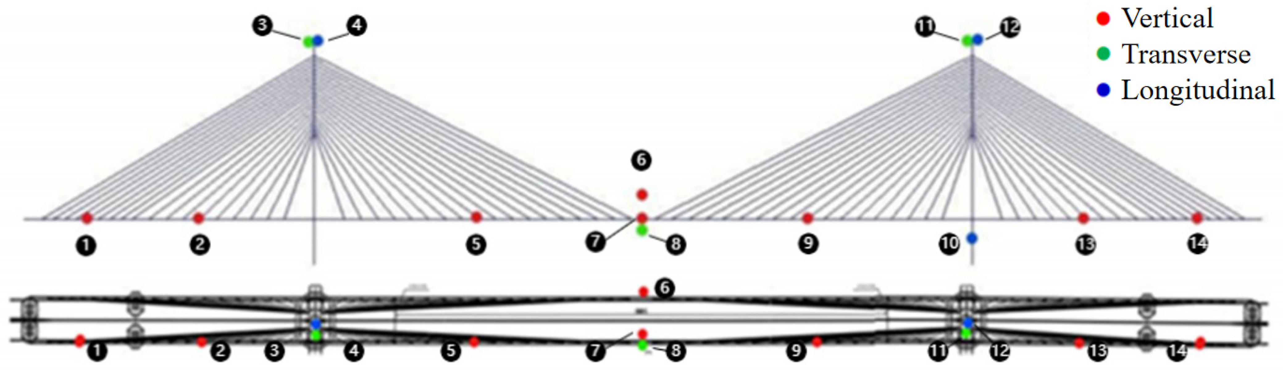
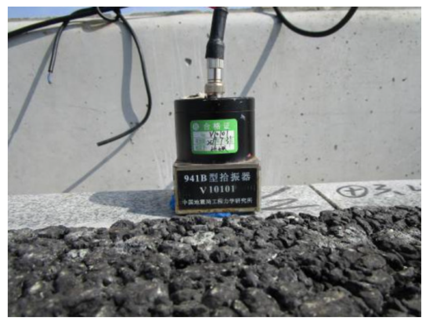
2. The Cable-Stayed Bridge and SHM System

The Poyang Lake Second Bridge, located in Lushan City, Jiangxi Province, spans the Duchang-Jiujiang Highway and is approximately 50 km away from the mouth of Poyang Lake in the Yangtze River. The length of the bridge is 5580 m. The main bridge consists of one main span and two side spans on each side, with a total length of 790 m along five spans (68.6 m + 116.4 m + 420 m + 116.4 m + 68.6 m). The bridge features two concrete towers, each with a height of 137.9 m, and two concrete piers on each side of two side spans. The bridge has double steel cable planes and a width of 28.0 m, with four traffic lane dual carriageways (Figure 1).

As indicated in Figure 2, the main bridge deck structure is composed of concrete deck over prefabricated steel frames. The steel frame consists of two separated steel I-section main girders, cross beams and secondary longitudinal beams, as shown in Figure 2a, which are assembled by joint plates and high-strength bolts. The two main girders are 26 m in length and are connected by cross beams. Three secondary longitudinal beams are installed between the two main girders, with spacings of 6 m, 7 m, and 7 m, respectively, followed by a final 6 m spacing. Low-shrinkage cast-in situ concrete is placed on the upper surface of the steel frame to form a steel–concrete composite bridge deck structure, as illustrated in Figure 2b.

There are two main pagoda-type concrete towers in the Poyang Lake Second Bridge, with a ratio of the main tower height to the main span of 0.256. The bridge consists of 72 pairs of cables arranged in a fan-shaped space with double cable planes. The cables connect the main bridge girders in a space of 10.8 m along the bridge’s main and side spans and link to the main tower in a vertical space of 10.8 m. The longest cable connecting at the midpoint of the main span is approximately 223 m. Six cable sizes are utilized for the cable’s cross sectional geometry using different amounts of high-strength steel wires, with a maximum cable diameter of 265 Φ 7 mm and a minimum cable diameter of 139 Φ 7 mm.

The SHM system of the Poyang Lake Second Bridge adopts comprehensive sensing techniques, signal processing approaches, computational algorithms and data processing methods. An advanced, stable, and efficient SHM system has been installed on the bridge to improve the reliability of bridge performance assessment and safety warning. Various types of sensors are utilized, including anemometers, thermometers, weigh-in-motion stations, accelerometers, strain gauges, GPS, load cells, and inclinometers. The sensory system installed on different functional components of the bridge is shown in Figure 3. The numbers in the brackets in Figure 3 denote the quantities of sensors installed at the relevant locations.

The instrumentation layout of the SHM system covers the main structural components of the Poyang Lake Second Bridge. On the basis of the geometric characteristics and structural behaviour of the bridge, the physical parameters in terms of real-time monitoring include environmental quantities (wind and temperature), load quantities (traffic load and traffic volume), structural response quantities (strain, acceleration, displacement and cable force), and structural variation quantities (settlement and tilt), as shown in

Table 1. Measuring parameters and sensors adopted for the SHM system.

Measuring Parameter	Sensor Type	Measuring Location	Sensor Number
Wind load	Anemometer	Main span midpoint, top tower	2
Ambient air temperature	Thermometer	Span midpoints, top tower	1
Highway traffic load	Weigh-in-motion station	Traffic loads	1
Vibration	Accelerometer	Main girders, top tower	14
Cable parameter	Accelerometer	Cables	76
Longitudinal displacement	Displacement transducer	Support bearings	4
Bridge desk deflection	Displacement transducer	Main girders	8
Stress distribution	Strain gauge	Main girders, cross beams	13
Cable tendon force	Load cell	Cable anchors	24
Geometry configuration	Inclinometer	Bridge piers	4

. The sensors were selected to ensure real-time health monitoring and performance assessment of the bridge. The placement of the sensors was appropriately selected to be at the critical points on the bridge, and the historic inspection data, finite element analysis results, structural risk analysis results, and recommendations by the relevant practising codes were considered.

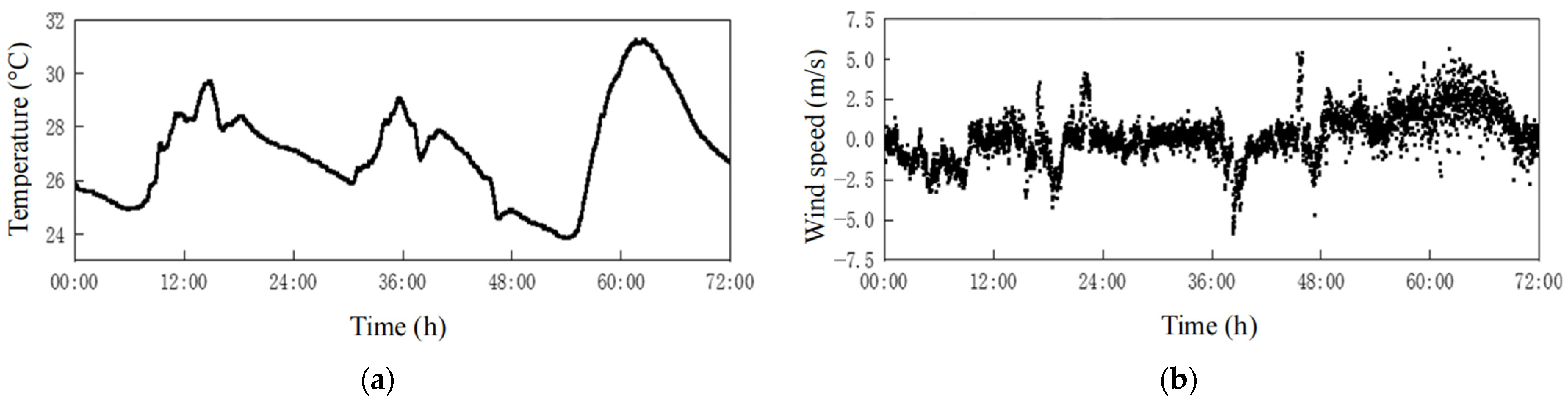
3. Monitored Data Analysis

A large amount of high-dimensional data are obtained from the installed sensory system, which can be utilized for various engineering applications after data pre-processing, such as traffic load analysis, structural behaviour evaluation, structural safety warning and operational modal analysis.

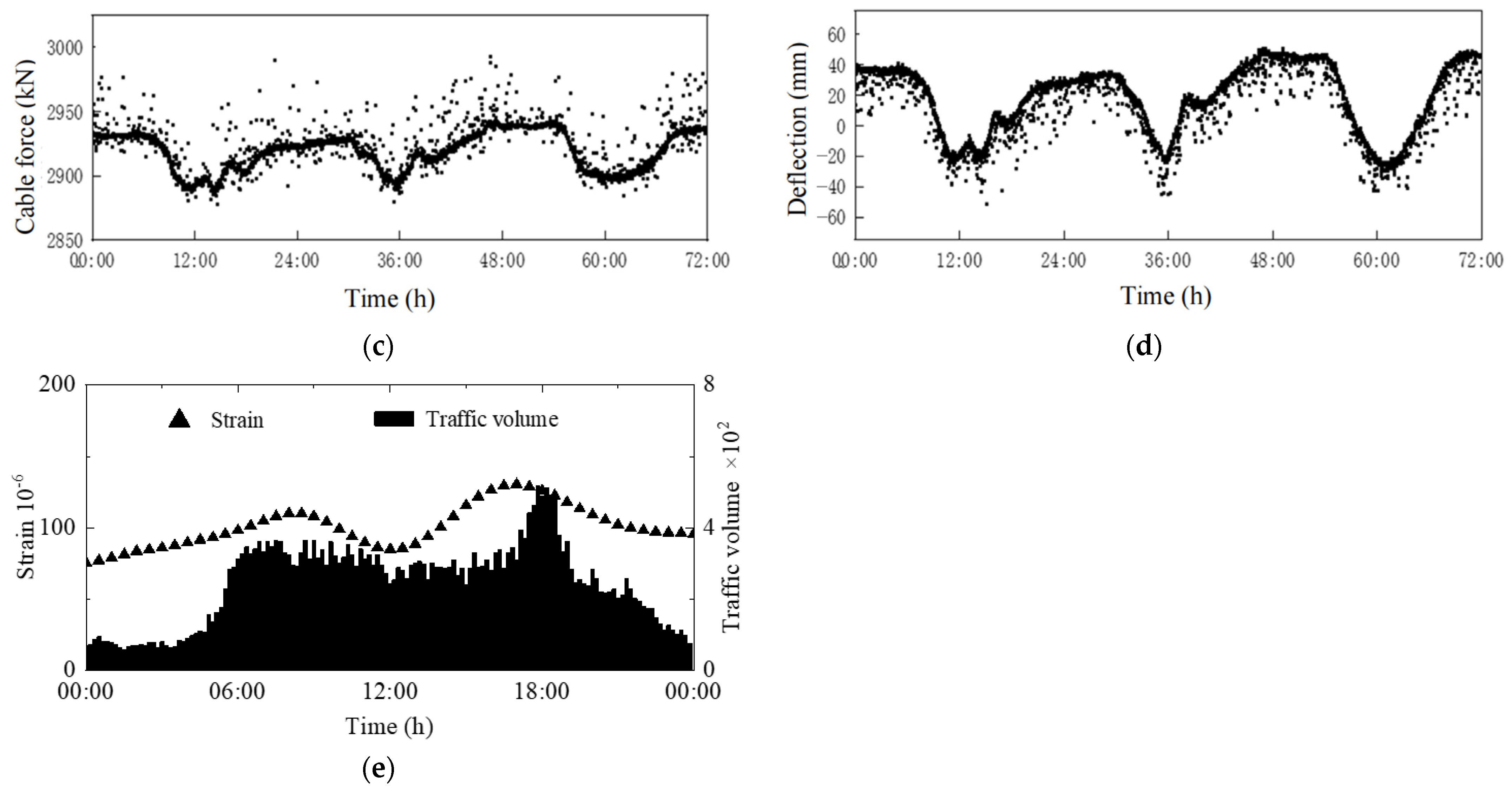
3.1. Traffic Statistics and Structural Response Analysis

The traffic volume of moving vehicles can be recorded continuously with installed weigh-in-motion systems and high-definition video cameras. From the recorded traffic data, the traffic volumes for the vehicles with different axle numbers can be statistically analyzed within a certain time period.

Table 2. Traffic volume statistics at different time periods for various vehicle axle numbers.

Time Period	2-Axle	3-Axle	4-Axle	5-Axle	>5-Axle	Total Number	Percentage
0:00–6:00	2662	126	97	34	263	3182	14.97%
6:00–12:00	4455	140	151	72	408	5226	24.59%
12:00–18:00	6147	142	117	48	472	6926	32.58%
18:00–24:00	4888	249	133	62	590	5922	27.86%
Total number	18,152	657	498	216	1733	21,256	100.00%
Percentage	85.40%	3.09%	2.34%	1.02%	8.15%	100.00%	/

summarizes the statistic results for moving vehicles during the time period between 17:00 on 2 January and 8:00 on 17 January 2020, with a total number of 21,256 recorded vehicles. From the results, the least number of vehicles passed during the time period 0:00–6:00 with a percentage of approximately 15%, and nearly a third of the vehicles passed during the time period 12:00–18:00, indicating heavy traffic volume in the afternoons.

The results of the SHM measurements of environmental quantities (e.g., ambient air temperature and lateral wind speed) and structural responses (e.g., cable force and bridge main girder deflection) of the bridge, which were recorded from 0:00 on 4 June to 24:00 on 7 June 2020, are provided in Figure 4. From the results, the temperature monitored at the midpoint of the main span changes over time on a daily basis, with the highest value around 2:00 p.m. and the lowest value around 6:00 a.m., as depicted in Figure 4a. The lateral wind speed varies randomly over time, with the highest values of 5.0 m/s in both the east and west directions, as shown in Figure 4b.

Figure 4c gives the SHM measurements for the cable force time history measured at CS01-01 on the cable connecting the main span bridge deck closest to the south bridge tower with the shortest length. From the results, the cable force varies over time, generally on a daily basis, with the highest value of approximately 3000 kN. Figure 4d presents the deflection time history recorded at HS005-01, a critical place in the bridge main span. The results indicate that the deflection varies over time within the range of −50 mm to 50 mm in a similar pattern to that of the cable force, which is mainly caused by the volume of traffic on a daily basis. Figure 4e presents the correlation between the WIM data and strain gauge data. The results show that as traffic volume increases, the amplitude of structural strain also increases accordingly. This demonstrates the significant impact of traffic loading on structural behaviour, which is crucial for understanding the in-service performance of the bridge.

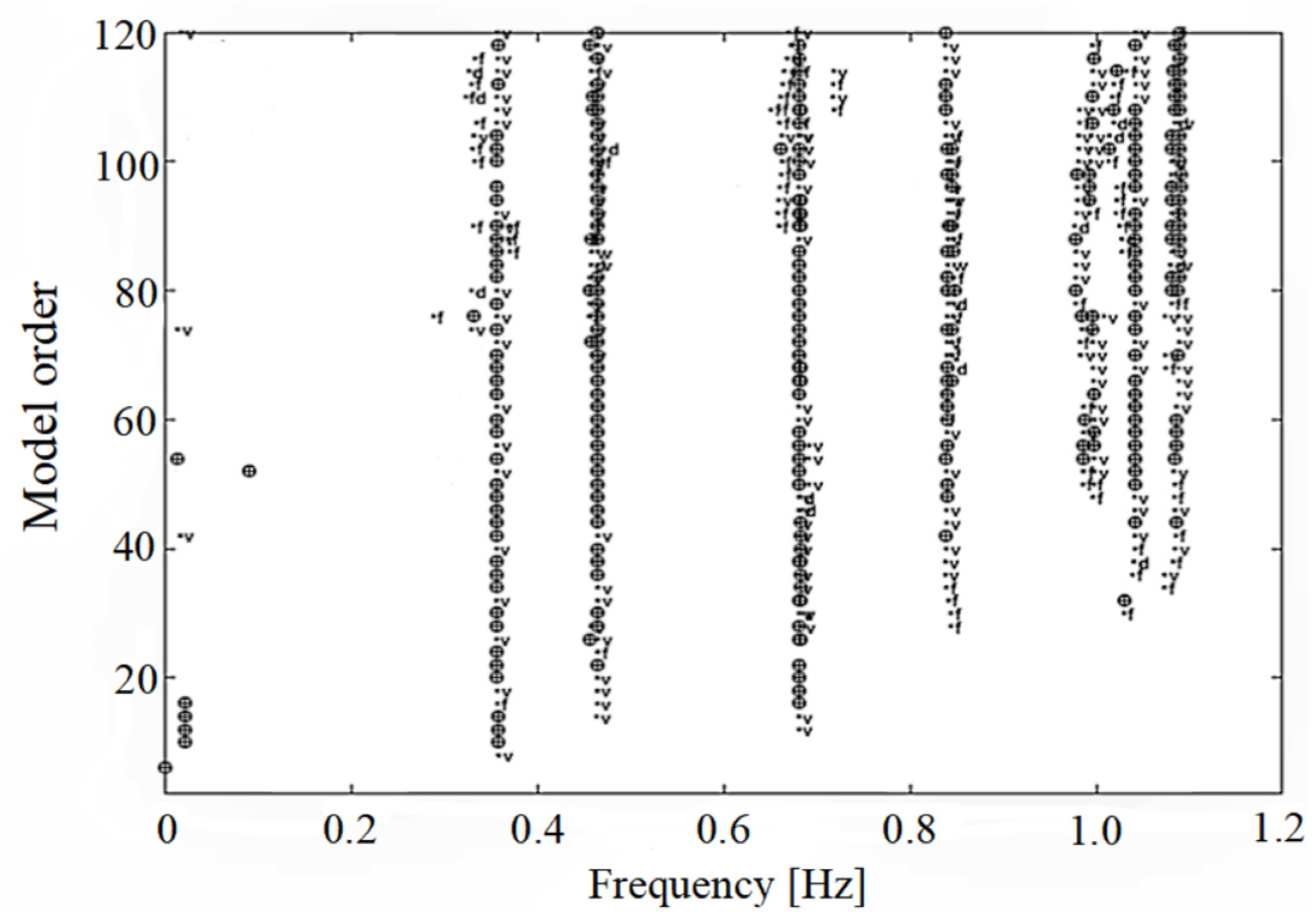
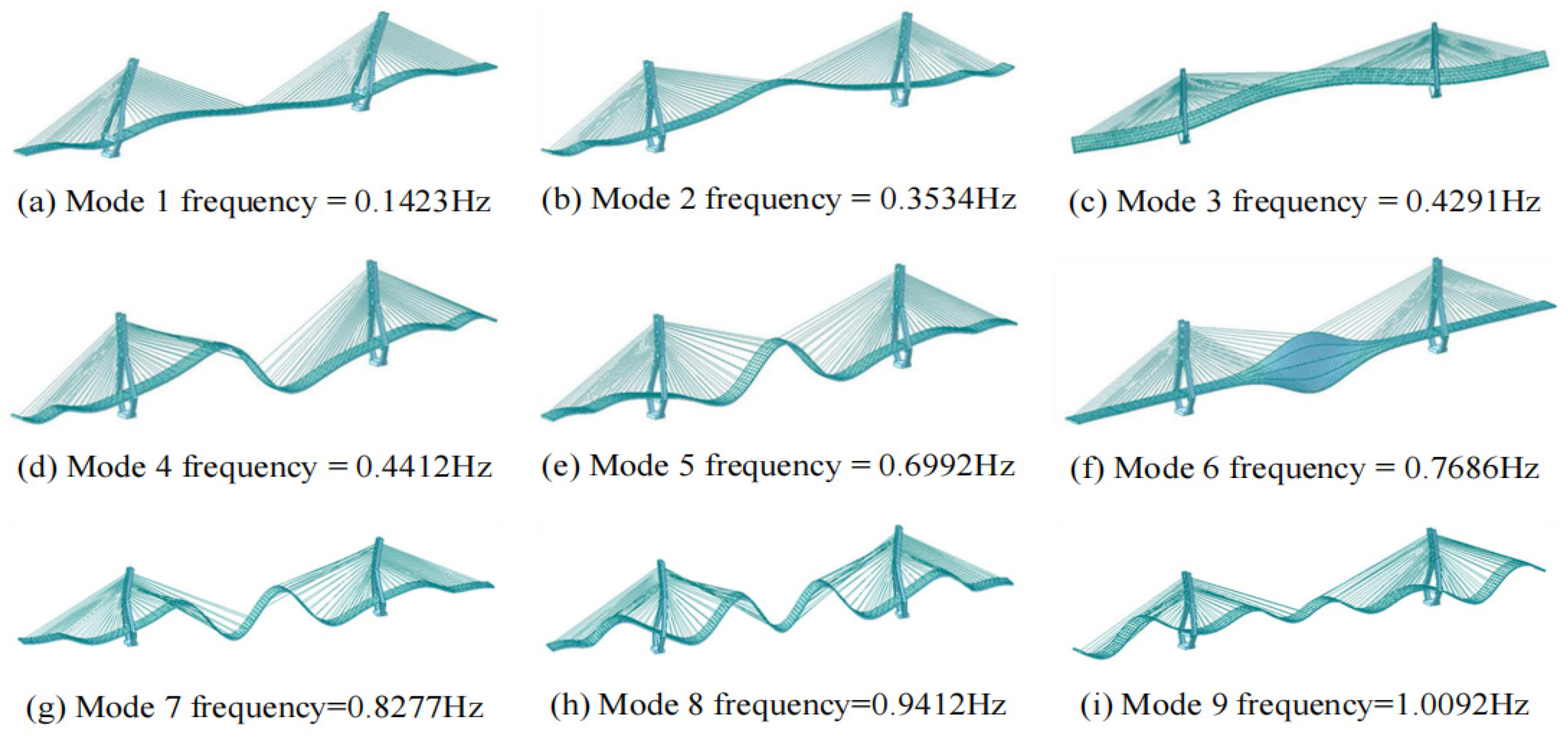
3.2. Operational Modal Analysis

Modal data identification is essential for bridge structural health monitoring and condition evaluation and serves as a valuable tool for structural dynamic performance analysis, structural damage identification, and FE model updating. By utilizing the measured ambient vibration data, modal parameters including natural frequencies and mode shapes can be extracted through appropriate operational modal analysis methods, such as the widely used stochastic subspace identification (SSI) methods [13,14].

Figure 5 illustrates the sensor layout used for the acceleration measurements. The sensing system was wired, with sensors placed at the midpoint and quarter points of the main span, as well as at the side spans and the top of the main towers. The numbers in Figure 5 represent the location indexes of the accelerometers. The numbers range from 1 to 14, indicating that a total of 14 Type 941B accelerometers were installed. This includes 8 accelerometers measuring vertical accelerations, 3 accelerometers measuring transverse accelerations, and an additional 3 accelerometers measuring longitudinal accelerations.

The accelerometers were selected for measuring the ambient acceleration responses, which can be utilized for operational modal analysis. A photo of the installed accelerometers is shown in Figure 6, and detailed information about the accelerometers is summarized in

Table 3. Technical specifications of the Type 941B accelerometers.

Item	Technical Specifications
Detection range	±2 g
Frequency response	0–120 Hz
Error	≤1%
Nonlinearity	≤1% FS
Sensitivity	≥2.5 V/g
Transverse sensitivity ratio	<1%
Dynamic range	>120 dB
Operating temperature	−40 °C to +85 °C

.

The acceleration time histories recorded by two accelerometers positioned at the midpoint of the main span and on the south side of the span are presented in Figure 7. The time period for the acceleration measurements ranges from 14:07 to 14:13 on 3 June 2020 with a total of 320 s, and the sampling frequency is set as 50 Hz, giving a total 16,028 available measured data for each sensor. From the results, the measured accelerations have values generally ranging from −0.15 m/s² to 0.15 m/s².

The SSI method, a time-domain approach, is widely utilized to extract modal properties from vibration data measurements. Typically, there are two techniques, i.e., data-driven SSI and covariance-driven SSI. In this study, the data-driven SSI method was adopted for extracting the natural frequencies of the bridge on the basis of the stabilization diagram, as shown in Figure 8. In the modal parameter extraction process, the maximum model order was set to 120, with a number of block rows of 80. The filtered stabilization diagram was then obtained in the low-frequency range below 1.2 Hz.

4. Finite Element Numerical Modelling

Three-dimensional (3D) full scale FE modelling was adopted for analyzing the dynamic properties of the Poyang Lake Second Bridge, and various types of elements were employed for different structural members to represent structural behaviour, which can be used for structural dynamic analyses.

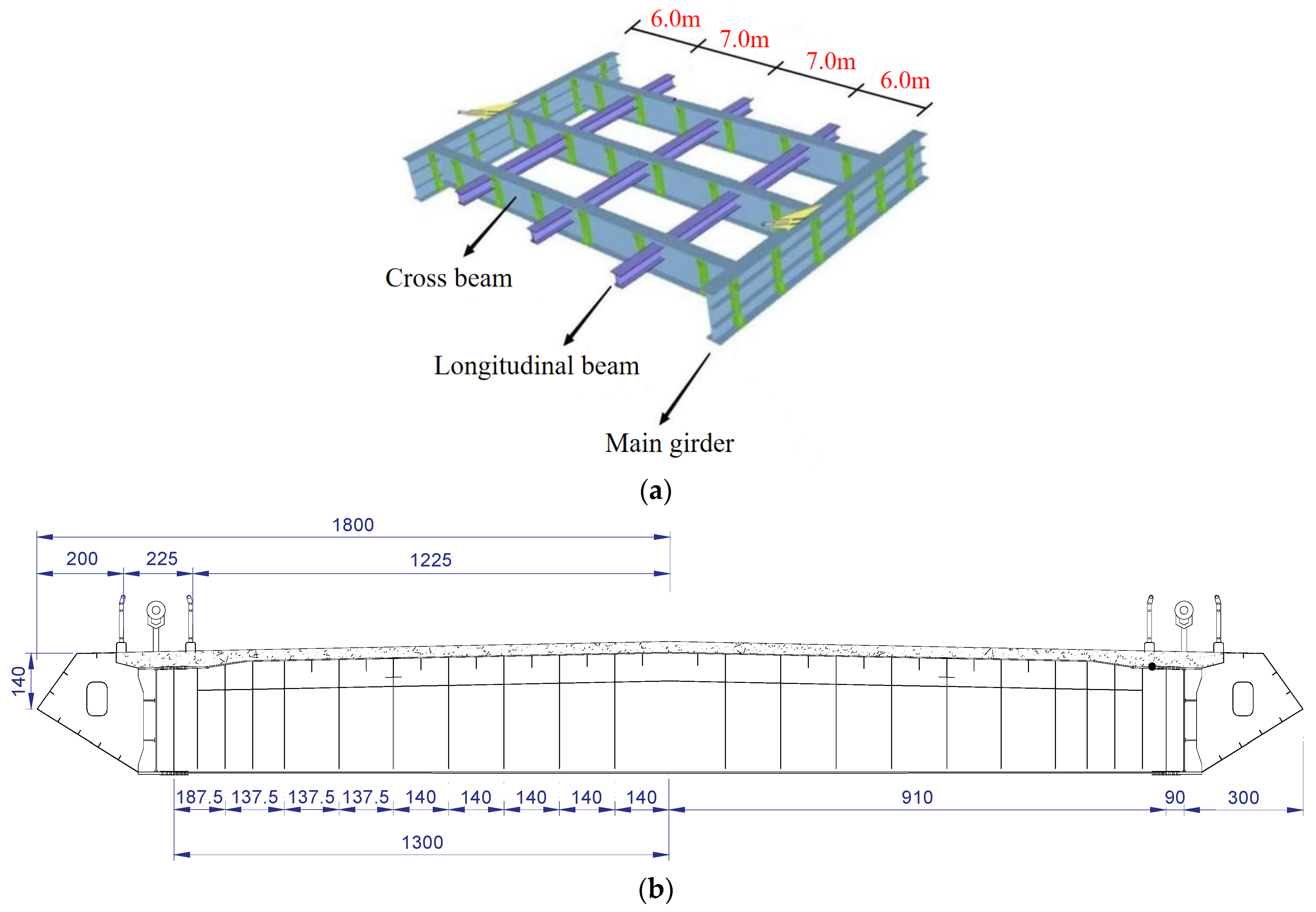
4.1. Geometric and Material Characteristics

On the basis of the design information, the geometric properties of the structural members and non-structural components of the bridge, including the dimensions of the girders, beams, towers and cables, are obtained, which can be utilized to construct the FE model. The material properties for each structural member of the cable-stayed bridge are initially estimated from the design, construction and maintenance data, as summarized in

Table 4. Material properties adopted for finite element numerical modelling.

Member Type	Elastic Modulus (GPa)	Poisson’s Ratio	Unit Weight (103 kN/m3)
Steel girder/beam	206	0.30	78.50
Concrete main tower	34.5	0.20	25.00
Concrete bridge pier	33.5	0.20	25.00
Concrete deck	35.5	0.20	25.00
Steel stay cable	195	0.30	78.50

. For example, the elastic modulus of concrete materials can be estimated from the concrete compressive strength by using the existing relation between the concrete elastic modulus and compressive strength, which should be verified by field tests.

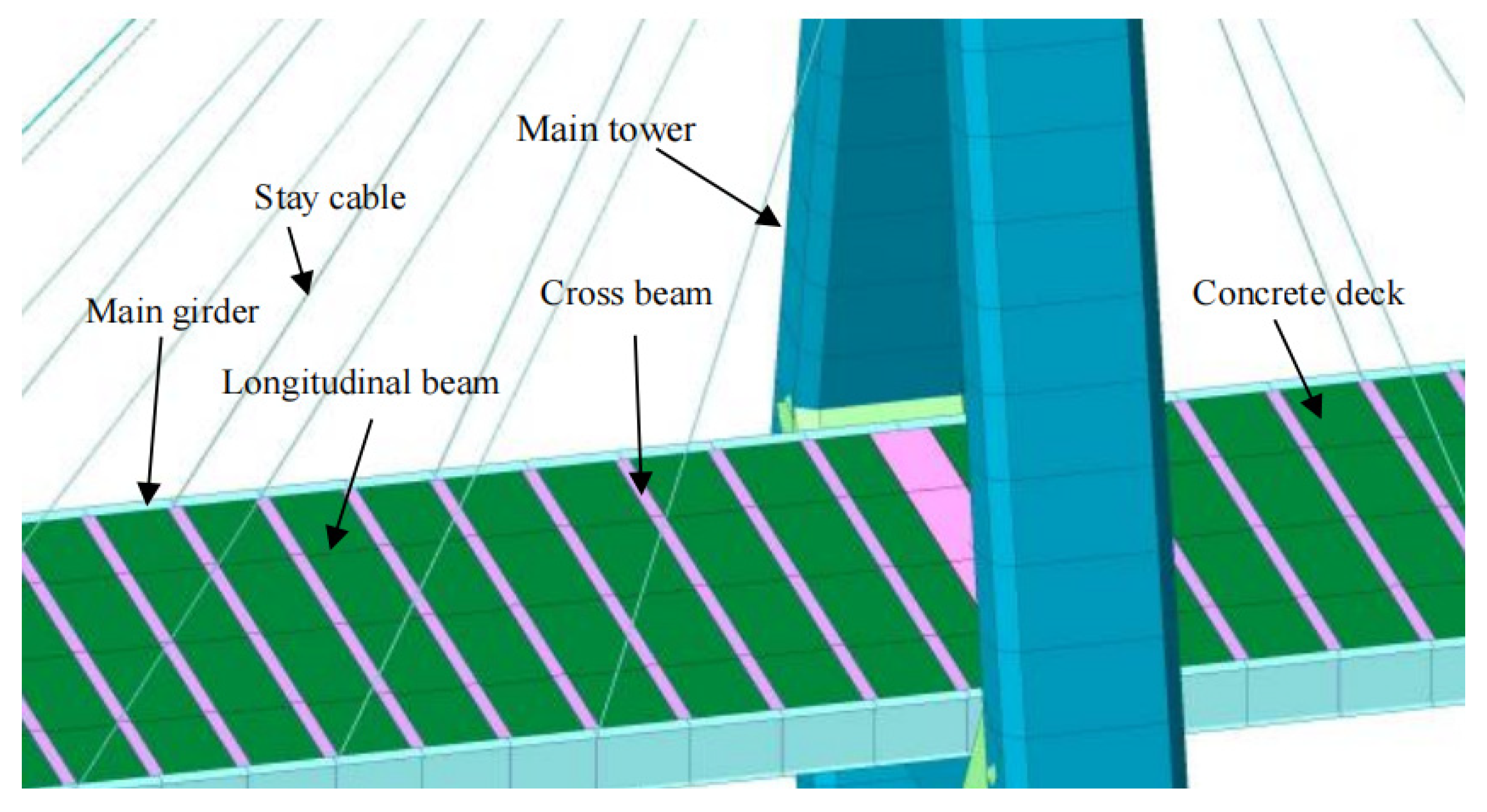
4.2. Finite Element Modelling

The FE model was constructed by the software ANSYS 18.1 [39]. In the FE model of the bridge deck structure, the steel frame consists of a central main beam aligned along the central axis of the bridge and two side main beams positioned within the cable planes, forming a framed structural component. These three main beams are then connected by cross beams that are linked by secondary longitudinal beams. Six-degree-of-freedom (6 DoF) beam elements are then utilized for the steel girders and beams and are also adopted for the concrete bridge main towers and side piers. For the concrete bridge deck, thin-wall shell elements are used to reflect the bridge deck behaviour. In the modelling of cables, tension-only truss elements are adopted, and the nonlinearity caused by the self-weight sag of the cables is also considered by updating the cable elastic modulus. To eliminate the nonlinear effect of the cable-stayed bridge self-weight, the Ernst formula is used to correct the elastic modulus of the cable, given as

$$E_{\mathrm{eq}}={\displaystyle \frac{E_{\mathrm{c}}}{1+\frac{E_{\mathrm{c}}\cdot {(r\cdot l)}^2}{12{\sigma }^3}}}$$

(1)

where $E_{\mathrm{eq}}$ is the updated elastic modulus; $E_{\mathrm{c}}$ is the elastic modulus of the cable; $l$ is the horizontal projection length; $r$ is the weight of the cable; and $\sigma$ is the stress of the cable.

Figure 9 shows the 3D FE model of the Poyang Lake Second Bridge. Here, a total number of 2172 beam elements, 880 shell elements and 144 tension-only truss elements are employed for constructing the numerical model. For the boundary and connection conditions of the cable-stayed bridge, the bridge main towers and side piers are assumed to be fixed on the basis of the actually constructed conditions, and all 6 DoF are constrained at the foundations. The connections between the main girders and the main towers or side piers are assumed to be constrained in vertical and lateral directions according to the actual situations, and the whole bridge is then free from longitudinal constraints.

4.3. Comparison of Experimental and Numerical Results

From the numerical model, the dynamic characteristics of the Poyang Lake Second Bridge are investigated. As depicted in Figure 10, the lower frequency modes of the bridge are presented. The analysis results show that the lowest frequency corresponding to the longitudinal floating mode is 0.1423 Hz, while the lowest frequency of the fundamental vertical bending mode is 0.3534 Hz.

To assess the accuracy of the modal characteristics obtained through FE modelling, the simulation results are then compared with the measured modal data identified from the monitored acceleration measurements.

Table 5. Comparison of numerical natural frequencies with measured data.

Mode Order	Numerical Result (Hz)	Measured Data (Hz)	Relative Error	Mode Description
1	0.1423	-	-	Longitudinal floating
2	0.3534	0.3605	−1.97%	1st symmetric vertical bending
3	0.4291	0.4437	−3.29%	1st lateral bending
4	0.4412	0.4649	−5.10%	1st anti-symmetric vertical bending
5	0.6992	0.6823	2.48%	2nd symmetric vertical bending
6	0.7686	0.7889	−2.57%	1st torsion
7	0.8277	0.8459	−2.15%	2nd anti-symmetric vertical bending
8	0.9412	0.9977	−5.66%	3rd symmetric vertical bending
9	1.0092	1.0426	−3.20%	3rd anti-symmetric vertical bending

summarizes the results obtained through numerical modelling as well as the identification results from the monitored acceleration test data. Due to the significant horizontal frictional effects of the supports in the bridge, the first-order longitudinal floating dynamic mode could not be identified from the measured acceleration data. Also, the lack of acceleration measurements in the direction of the bridge longitudinal floating affects the floating mode identification.

As indicated in Table 5, the relative errors between the numerical results and the corresponding measured natural frequencies range from −5.66% to 2.48%, with an average absolute relative error of 3.30%. The dynamic frequencies obtained from the numerical modelling show a high degree of consistency with the measured modal data. This indicates that the numerical model can accurately reflect the dynamic behaviour of the constructed Poyang Lake Second Bridge.

5. Model Updating

As indicated by the modal data obtained from the monitored data and numerical modelling for the bridge, as shown in Table 5, there is a notable discrepancy between the measured frequencies and those obtained from numerical simulations. This discrepancy indicates the presence of potential modelling errors in the numerical simulation for the bridge, as well as possible measurement uncertainties in the monitored vibration data. To address these discrepancies, a model updating process is needed. By utilizing the measured modal dada, such as natural frequencies, the FE numerical model can be adjusted to enhance the correlation between the actual bridge structure and its FE model.

5.1. Model Updating Theory

Due to the material and geometric complexities of the actual bridge, uncertainties are usually present in the modelling of the stiffness and mass properties of the actual structure. The uncertainties of the model are predominantly related to the difference in stiffness ($\Delta K$) and mass ($\Delta M$) between the actual bridge structure and its numerical model.

For the numerical model with the global stiffness matrix ($K$) and mass matrix ($M$), the corresponding global stiffness matrix ($\tilde{K}$) and mass matrix ($\tilde{M}$) of the actual structure, which has a total of Nm degrees of freedom, can be formulated as follows

$$\Delta K=\tilde{K}-K,\Delta M=\tilde{M}-M$$

(2)

In practice, the measured mode shapes of the long-span bridge structure are often incomplete due to the limited number of sensors installed. Consequently, the eigenvectors of the actual structure can be approximated by using the corresponding numerical eigenvectors. Here, only natural frequencies are considered in the process of model updating due to the difficulty of obtaining full mode shapes. By using mass normalization of the numerical eigenvectors, the dynamic characteristic equation is rewritten as [25]

$${\displaystyle \frac{{{\mathbf{\varphi }}_i}^T(\Delta K-{{\widehat{\omega }}_i}^2\Delta M){\mathbf{\varphi }}_i}{{{\widehat{\omega }}_i}^2-{{\omega }_i}^2}}=1$$

(3)

where ${\omega }_i$ and ${\widehat{\omega }}_i$ are the ith frequency of the numerical model and the related real structure, respectively; ${\mathbf{\varphi }}_i$ and ${\widehat{\mathbf{\varphi }}}_i$ are the ith eigenvector of the numerical model and the related real structure, respectively.

The difference in stiffness ($\Delta K$) and mass ($\Delta M$) between the FE numerical model and the associated actual structure can be expressed as

$$\Delta K={\displaystyle \sum _{j=1}^{N\alpha }{\alpha }_j{K}_j},\Delta M={\displaystyle \sum _{j=1}^{N\beta }{\beta }_j{M}_j}$$

(4)

where ${\alpha }_j$ and ${\beta }_j$ are parameters for structural stiffness and mass updating, respectively, characterized by a structural element or a structural member group; $N\alpha$ and $N\beta$ are the total number of structural updating parameters, respectively; and $K_j$ and $M_j$ represent the contributions made by the jth group or element to the system stiffness and mass, respectively.

By incorporating the structural updating parameters as defined in Equation (4), Equation (3) for the ith dynamic mode is now written as

$${\displaystyle \frac{{\displaystyle \sum _{j=1}^{N\alpha }{a}_{ij}{\alpha }_j-{{\widehat{\omega }}_i}^2{\displaystyle \sum _{j=1}^{N\beta }{b}_{ij}{\beta }_j}}}{{{\widehat{\omega }}_i}^2-{{\omega }_i}^2}}=1$$

(5)

where $a_{ij}={{\mathbf{\varphi }}_i}^T{K}_j{\mathbf{\varphi }}_i$ and $b_{ij}={{\mathbf{\varphi }}_i}^T{M}_j{\mathbf{\varphi }}_i$ are the sensitivity coefficients that are related to the ith eigenmode and the jth contribution, respectively.

When the total number Nm of measured dynamic modes for the actual bridge structure is available, e.g., Nm measured frequencies available, the governing equation in Equation (5) can be adopted to provide the total number of Nm equations, so as to find a solution for a total of ($N\alpha$+$N\beta$) of the stiffness and mass updating parameters. By using the measured Nm frequencies, Equation (5) is now expressed in a matrix form as

$$A\alpha -\Omega B\beta -f=0$$

(6)

where $A$ and $B$ are the coefficient matrices composed of the sensitivity coefficients $a_{ij}$ and $b_{ij}$, respectively; $\alpha$ and β represent the unknown vectors for the chosen structural stiffness and mass updating parameters, respectively; $\Omega$ represents the diagonal matrix containing the measured Nm frequencies; and the known coefficient vector $f$ comprises elements $f_i={{\widehat{\omega }}_i}^2-{{\omega }_i}^2$ for i = 1, …, Nm.

In this study, the Tikhonov regularization algorithm [20] is utilized to obtain a reliable solution for the updating parameters, by minimizing the effect of measurement uncertainties on the structural model updating process. Based on the governing equation presented in Equation (6), the Tikhonov regularization solution for these updating parameters can be represented with a constrained optimization problem.

The Tikhonov regularization parameter θ can be solved by using the L-curve criterion [25,40]. This method does not need a priori information of the noise level in the measured data. The L-curve is a log–log plot of the residual norm $\rho (\theta )$ and the solution norm $\eta (\theta )$, defined as

$$\rho (\theta )={‖W[A\alpha (\theta )-\Omega B\beta (\theta )-f]‖}^2={\displaystyle \sum _{j=1}{[\frac{{\theta }^2}{{{\sigma }_j}^2+{\theta }^2}{u_j}^T{f}_w]}^2}$$

(7a)

$$\eta (\theta )={‖\alpha (\theta )‖}^2+{‖\beta (\theta )‖}^2={\displaystyle \sum _{j=1}{[\frac{{\sigma }_j}{{{\sigma }_j}^2+{\theta }^2}{u_j}^T{f}_w]}^2}$$

(7b)

where ${\sigma }_j$ is the jth singular value (j = 1 ~ $N\alpha +N\beta$); $u_j$ and $v_j$ represent the jth left and right orthogonal column vectors, respectively, derived from the singular value decomposition of the known sensitivity coefficient matrix, which is presented here as

$${\displaystyle \sum _{j=1}{\sigma }_j{u}_j{v_j}^T}=\left[\begin{array}{cc}WA& 0\\ 0& -W\Omega B\end{array}\right]$$

(8)

Research has shown that the corner of the L-curve, where the L-curve has an approximate maximum curvature, offers an optimal regularization parameter that balances the residual norm error and the solution norm error [40]. Based on Equation (7), the curvature of the L-curve $\kappa (\theta )$ is expressed as

$$\kappa (\theta )={\displaystyle \frac{2\eta \rho }{{\eta }^{\prime }}}{\displaystyle \frac{({\theta }^2{\eta }^{\prime }\rho +2\theta \eta \rho +{\theta }^4\eta {\eta }^{\prime })}{{({\theta }^4{\eta }^2+{\rho }^2)}^{3/2}}}$$

(9)

where ${\eta }^{\prime }$ represents the first derivative of η with respect to θ. Consequently, the optimal regularization parameter θ can be obtained through an optimization algorithm by using Equation (9).

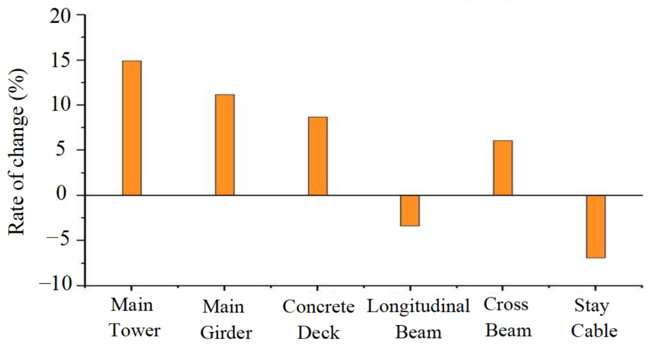
5.2. Structural Parameters for Updating

For a complex cable-stayed bridge, it is challenging to utilize a large number of model updating parameters for updating the FE numerical model, since the information available on the measured modal data is often limited. Therefore, the structural members with the same type and function could be grouped and updated by using a shared model updating parameter.

For the cable-stayed Poyang Lake Second Bridge, a total of six structural member groups are selected for dynamic model updating, e.g., steel main girders, steel cross beams, steel longitudinal beams, steel stay cables, concrete bridge decks, and concrete towers and piers, as shown in Figure 11. Here, a scalar multiplier is employed for the stiffness updating characterized at each structural member group, representing the change rate of stiffness for the structural member group, and the mass characteristics are not considered due to their relatively higher accuracy. Consequently, only stiffness updating parameters ${\alpha }_j$ are required to be updated and solved in the optimization problem.

5.3. Updated Numerical Model

In this paper, the regularized model updating method is applied to update the constructed FE model of the Poyang Lake Second Bridge. For the model updating, a total of eight measured natural frequencies are used.

Table 6. Comparative analysis of initial and updated natural frequencies of the cable-stayed bridge.

Mode	Numerical Frequency (Hz)	Measured Frequency (Hz)	Initial Error (%)	Updated Frequency (Hz)	Updated Error (%)
2	0.3534	0.3605	−1.97%	0.3560	−1.24%
3	0.4291	0.4437	−3.29%	0.4413	−0.54%
4	0.4412	0.4649	−5.10%	0.4686	0.79%
5	0.6992	0.6823	2.48%	0.6884	0.89%
6	0.7686	0.7889	−2.57%	0.8005	1.47%
7	0.8277	0.8459	−2.15%	0.8367	−1.09%
8	0.9412	0.9977	−5.66%	0.9875	−1.02%
9	1.0092	1.0426	−3.20%	1.0264	−1.55%

presents a summary of the updated frequencies by comparing with the initial calculated frequencies. In this study, the regularization algorithm is utilized to eliminate the influence of uncertainties associated with frequency measurements. In the optimization procedure for the model updating, the upper and lower bounds of the stiffness updating parameters are chosen as $20\%\ge {\alpha }_j\ge -20\%$. As a result, a robust and optimal solution for the stiffness updating parameters is obtained after only few iterations.

As indicated in Table 6, the updated numerical frequencies show significant improvement in relation to the measured frequencies obtained from the monitored vibration data. After the model updating process, the average absolute relative error has been substantially reduced from 3.30% to 1.08%.

The updated stiffness parameters of the FE model for the cable-stayed bridge are illustrated in Figure 12, by utilizing data from eight measured frequencies. The results show that the stiffness updating parameters, which reflect the change rate of stiffness for each structural member group, range from −7.14% and 14.88%, with an average absolute value of 8.59%.

In practice, the results seem reasonable since relatively minor adjustments to the stiffness in the initial numerical model are needed to minimize the difference between the numerically predicted frequencies and the measured frequencies.

6. Damage Identification

6.1. Damage Scenarios Assumed

To effectively identify damage in the cable-stayed bridge, since the measured modal data available are typically very limited in practice, the updated 3D full scale finite element numerical model is now reduced to a two-dimensional finite element model by the equivalent stiffness approach and model reduction method [41], as shown in Figure 13. In this study, the main span deck is discretized into 76 segments, comprising a total of 77 nodes. These nodes are critical reference points for conducting structural damage identification.

Since no notable structural damage has been observed in the Poyang Lake Second Bridge, two damage scenarios are simulated here to undertake the inverse identification of potential structural damage. In the damage scenario 1, the main span bridge deck is simulated to be damaged. This bridge deck damage is situated at the centre of the main span, specifically in segment 39 which lies between nodes 39 and 40. The damage scenario 2 simulates the multiple bridge deck damage in the south side span located at segment 14 between nodes 14 and 15, in addition to the damage for scenario 1. In this study, the damage to the structural elements of the main span bridge deck is simulated by assuming a reduction in the stiffness of structural members, while the mass remains unchanged. Modal data, including mode shapes for the damaged structure, are adopted for structural damage identification, which can be obtained through the dynamic analysis of the numerical model with the simulated damage.

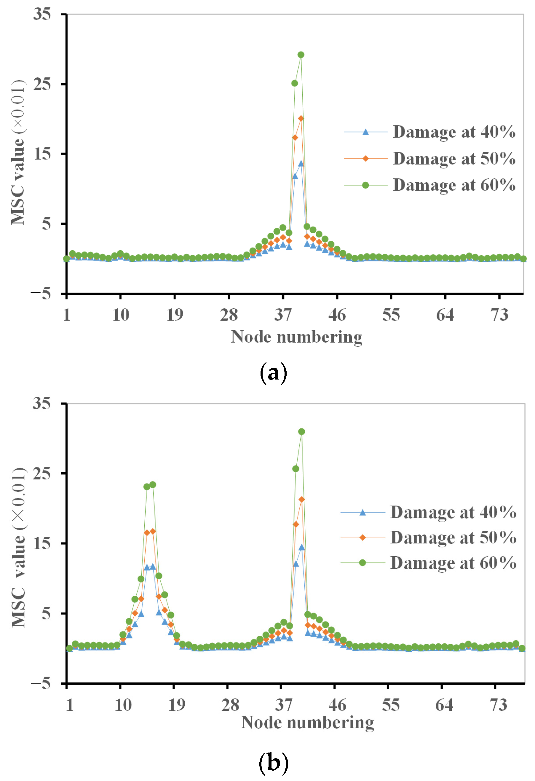
6.2. Mode Shape Curvature Method

The mode shape curvature (MSC) method for damage identification is based on the fact that changes in MSC are highly concentrated at the location where damage occurs. This curvature can be computed from the measured mode shapes using a central difference approximation [41]. Subsequently, the change in MSC is considered as a key indicator for detecting and locating structural damage. When a total of Nm mode shapes are accessible, the MSC damage index at position j can be defined as the average of the absolute values of the curvature change rates for all Nm modes, namely

$$\mathrm{MSC}(j)={\displaystyle \frac{1}{Nm}}{\displaystyle \sum _{i=1}^{Nm}\frac{\left|C_i^{\mathrm{d}}(j)-C_i^{\mathrm{u}}(j)\right|}{{\displaystyle \sum _j\left|C_i^{\mathrm{d}}(j)-C_i^{\mathrm{u}}(j)\right|}}}$$

(10)

where $C_i^{\mathrm{u}}(j)$ and $C_i^{\mathrm{d}}(j)$ represent the mode shape curvatures for the undamaged structure and damaged structure at location j for the ith mode, respectively, defined here as

$$C_i^u(j)={\displaystyle \frac{{{\mathbf{\varphi }}_i}^{\mathrm{u}}(j+1)}{\Delta l^2}}-\left[{\displaystyle \frac{2{{\mathbf{\varphi }}_i}^{\mathrm{u}}(j)-{{\mathbf{\varphi }}_i}^{\mathrm{u}}(j-1)}{\Delta l^2}}\right]$$

(11a)

$$C_i^{\mathrm{d}}(j)={\displaystyle \frac{{{\mathbf{\varphi }}_i}^{\mathrm{d}}(j+1)}{\Delta l^2}}-[{\displaystyle \frac{2{{\mathbf{\varphi }}_i}^{\mathrm{d}}(j)}{\Delta l^2}}-{\displaystyle \frac{{{\mathbf{\varphi }}_i}^{\mathrm{d}}(j-1)}{\Delta l^2}}]$$

(11b)

where ${\mathbf{\varphi }}_i(j-1)$, ${\mathbf{\varphi }}_i(j)$ and ${\mathbf{\varphi }}_i(j+1)$ represent the values of the ith mode shape at the (j − 1)th, jth, and (j + 1)th nodes, respectively, and Δl indicates the interval between two adjacent nodes.

The MSC damage index is utilized to identify the simulated damage scenarios within the structure. Figure 14 presents the correlation between the MSC damage index values and the segment numbers for these two simulated damage scenarios. A total number of 10 simulated damaged mode shapes are used for the inverse damage identification, and different levels of assumed damage amounts are considered, i.e., 40%, 50%, and 60%, respectively. In the case of damage scenario 1, where damage is simulated at segment 39 with nodes 39 and 40, as illustrated in Figure 14a, the results demonstrate that a significant MSC damage index value exists at nodes 39 and 40. This elevated value effectively identifies the damage location at segment 39 for the simulated damage scenario 1. Furthermore, the MSC damage index value increases as the damage amount increases, giving more obvious identification of the simulated damage.

Figure 14b illustrates the results of inverse identification for multiple aspects of damage using the MSC damage index. From the results, the MSC damage index gives significant values at nodes 39 and 40 as well as at nodes 14 and 15, correctly showing the damage locations at segments 39 and 14 for the simulated multiple damage aspects. Again, the MSC damage index becomes greater with the increase in damage amount, indicating that more severe structural damage could be identified more clearly.

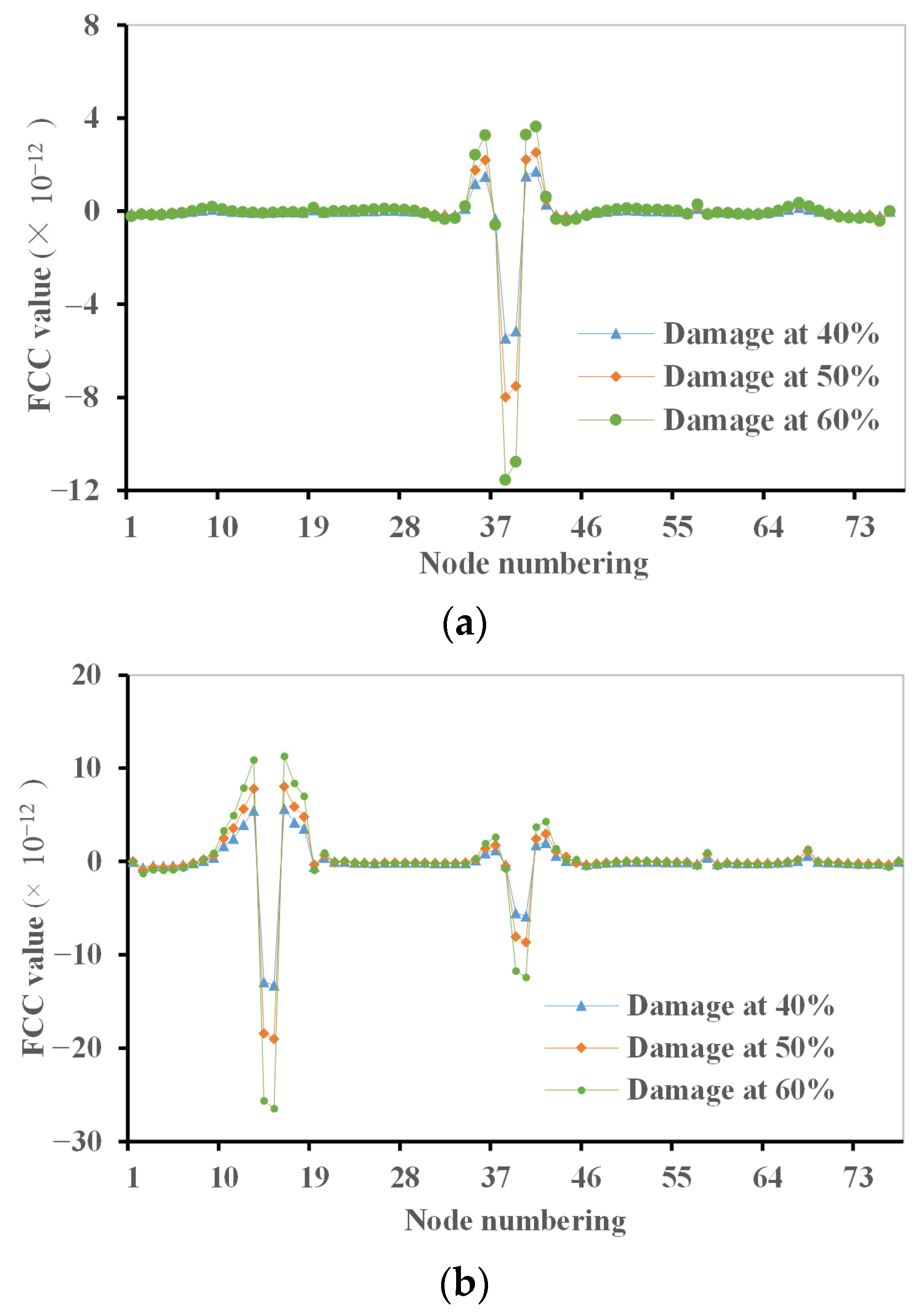
6.3. Flexibility Change Curvature Method

The flexibility change curvature (FCC) method assumes that the flexibility matrix of a dynamic structure can be directly computed from its frequencies and mode shapes. It suggests that an accurate approximation of the flexibility matrix can be derived from a limited number of lower-frequency modes. Consequently, structural damage that induces changes in flexibility can be directly identified using the measured modal data. Thus, structural damage related to the change in flexibility can be identified directly using the measured modal data [37]. The FCC damage index at the jth DoF can be defined as

$$\mathrm{FCC}(j)={\displaystyle \frac{\delta {\tilde{f}}_{j+1}+\delta {\tilde{f}}_{j-1}}{\Delta l_{j-1}\Delta l_{j+1}}}-{\displaystyle \frac{2\delta {\tilde{f}}_j}{\Delta l_{j-1}\Delta l_{j+1}}}$$

(12)

where $\Delta l_{j-1}$ and $\Delta l_{j+1}$ are the distance between the nodes with the (j − 1)th and jth DoF and the distance between the nodes with the jth and (j + 1)th DoF, respectively, while $\delta {\tilde{f}}_{j+1}$, $\delta {\tilde{f}}_j$ and $\delta {\tilde{f}}_{j-1}$ are the maximum absolute value of the elements in the (j − 1)th, jth and (j + 1)th columns of the matrix of flexibility change between the undamaged and damaged structure, respectively, characterized as

$$\delta {\tilde{f}}_j=\underset{i}{\max }\left|\delta f_{ij}\right|=\underset{i}{\max }\left|f_{ij}^{\mathrm{u}}-f_{ij}^{\mathrm{d}}\right|$$

(13)

in which $\delta f_{ij}$ are the entries of the change in the flexibility matrix $\Delta F$ between the structure in the undamaged and damaged state, obtained from

$$\Delta F=F^{\mathrm{u}}-F^{\mathrm{d}}$$

(14)

where $F^{\mathrm{u}}$ and $F^{\mathrm{d}}$ denote the flexibility matrices of the original and damaged structures, respectively. When the first Nm modes are available, the flexibility matrices for both the original and damaged structures can be, respectively, approximated from

$$F^{\mathrm{u}}={\displaystyle \sum _{i=1}^{Nm}\frac{1}{{\left({\omega }_i^{\mathrm{u}}\right)}^2}{\mathbf{\varphi }}_i^{\mathrm{u}}}{\left({\mathbf{\varphi }}_i^{\mathrm{u}}\right)}^T, F^{\mathrm{d}}={\displaystyle \sum _{i=1}^{Nm}\frac{1}{{\left[{\omega }_i^{\mathrm{d}}\right]}^2}{\mathbf{\varphi }}_i^{\mathrm{d}}}{\left({\mathbf{\varphi }}_i^{\mathrm{d}}\right)}^T$$

(15)

The quantity $\mathrm{FCC}(j)$ can be used as an index for quantifying the FCC at each measurement location. Similarly to the MSC method, the damage identification process of the FCC method does not require an analytical or numerical model.

Figure 15 presents the results of the inverse damage identification from the FCC method, where two simulated damage scenarios with various damage extents are considered. A total of the first three modes of the damaged structure are utilized for calculating the FCC damage index. For the case with a single aspect of damage in the centre of the main span at segment 39, the results in Figure 15a show significant FCC damage index changes at nodes 39 and 40 of segment 39, and these changes are more obvious for the cases with higher damage extents, indicating that the single aspect of damage is correctly identified by the FCC method.

For the case of simulated damage scenario 2, where the damage is located at multiple locations, i.e., in the centre of the main span at segment 39 with nodes 39 and 40 and on the south side span at segment 14 with nodes 14 and 15, the results in Figure 15b provide good indications for the multiple aspects of damage by using the FCC method. The two locations of the multiple aspects of damage are clearly identified at nodes 39 and 40 as well as at nodes 14 and 15, and the severity of the multiple aspects of damage is also indicated depending on the assumed damage extent.

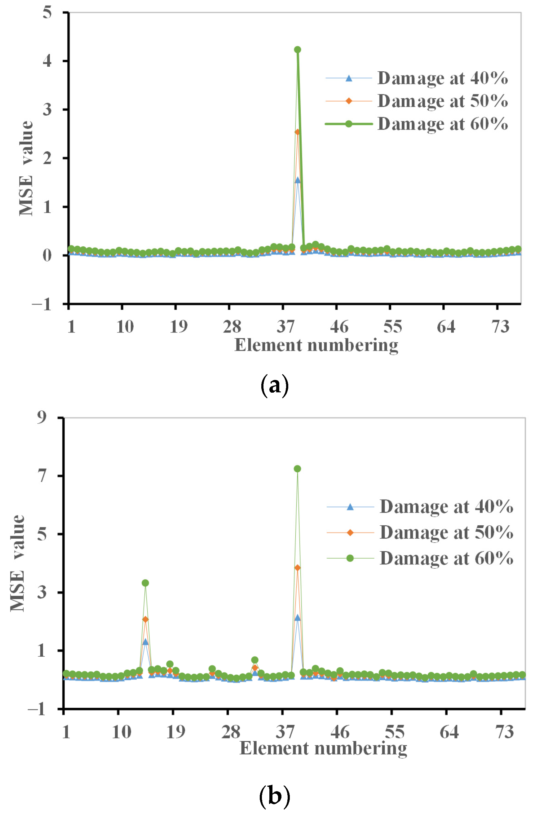
6.4. Modal Strain Energy Method

In the case of beam-type structures, the modal strain energy (MSE) can be adopted as a useful indicator for damage detection. The approach involves the assessment of the changes in MSE before and after the occurrence of damage, since structural damage can cause a decrease in the flexural rigidity at the site where the damage occurs [41]. When there is a total of Nm mode shapes available, the damage index for the jth element is considered as the mean value of the absolute change rates of the MSE for all Nm modes, i.e.,

$$\mathrm{MSE}(j)={\displaystyle \frac{1}{Nm}}{\displaystyle \sum _{i=1}^{Nm}\frac{\left|U_{ij}^{\mathrm{d}}-U_{ij}^{\mathrm{u}}\right|}{U_{ij}^{\mathrm{u}}}}$$

(16)

where $U_{ij}^{\mathrm{u}}$ and $U_{ij}^{\mathrm{d}}$ are the strain energy of the jth element for the ith mode for the original and damaged structures, respectively, defined as

$$U_{ij}^{\mathrm{u}}={\left({\mathbf{\varphi }}_i^{\mathrm{u}}\right)}^T{K}_j^{\mathrm{u}}{\mathbf{\varphi }}_i^{\mathrm{u}}, U_{ij}^{\mathrm{u}}={\left({\mathbf{\varphi }}_i^{\mathrm{d}}\right)}^T{K}_j^{\mathrm{d}}{\mathbf{\varphi }}_i^{\mathrm{d}}$$

(17)

in which $K_j^{\mathrm{u}}$ and $K_j^{\mathrm{d}}$ represent the element stiffness matrices for the jth element in the original and damaged structures, respectively, and are presented as

$$K_j^{\mathrm{u}}=E_j^{\mathrm{u}}{K}_{j0}, K_j^{\mathrm{d}}=E_j^{\mathrm{d}}{K}_{j0}$$

(18)

where $E_j^{\mathrm{u}}$ and $E_j^{\mathrm{d}}$ are the parameters signifying the material stiffness properties of the jth element in the original and damaged structures, respectively; the matrix $K_{j0}$ is only determined by geometric quantities. Thus, the MSE damage index at jth element in Equation (16) is expressed here as

$$\mathrm{MSE}(j)={\displaystyle \frac{1}{Nm}}{\displaystyle \sum _{i=1}^{Nm}\left|1-\frac{E_j^{\mathrm{d}}}{E_j^{\mathrm{u}}}•\frac{{\left({\mathbf{\varphi }}_i^{\mathrm{d}}\right)}^T{K}_{j0}{\mathbf{\varphi }}_i^{\mathrm{d}}}{{\left({\mathbf{\varphi }}_i^{\mathrm{u}}\right)}^T{K}_{j0}{\mathbf{\varphi }}_i^{\mathrm{u}}}\right|}$$

(19)

The MSE method is utilized to identify the locations of these two simulated damage scenarios, as illustrated in Figure 16. The first 10 modes of the damaged structure are employed in the inverse damage identification process. The extent of damage is simulated by reducing the stiffness of the structural members. Figure 16a provides the results for the MSE damage index values at each segment of the bridge deck, where the damage scenario 1 in the centre of the main span is considered. From the results, the damage location is correctly identified at segment 39, and the damage severity is also indicated by the MSE damage index values.

For the case with damage scenario 2 at multiple locations, i.e., in the centre of the main span at segment 39 and on the south side span at segment 14, Figure 16b shows the results for the MSE damage index value against the bridge deck segment number. From the results, both damage placements are correctly identified at the simulated positions at segments 39 and 14. Here again, the MSE damage index value increases obviously as the damage amount increases.

7. Conclusions

This paper investigates the SHM system adopted for the cable-stayed Poyang Lake Second Bridge and analyses the monitored data for structural behaviour assessment, finite element modelling, dynamic model updating and structural damage recognition. The structural monitoring system adopted for the bridge is studied, and the monitored data are investigated for environmental effects, structural performance and modal data extraction. From the measured modal data, the regularized model updating method is utilized to update the FE model. Finally, various vibration-based structural damage identification methods can accurately identify the simulated damage in the cable-stayed bridge from the calibrated numerical model. Based on the obtained results, the following conclusions are drawn:

(1)

The implemented SHM system provides useful information for dynamic performance evaluation, numerical model updating and structural condition assessment. The structural parameters, such as cable forces and bridge deck deflections of the cable-stayed bridge, vary over time and can be affected by environmental factors and traffic loads.

(2)

The initial FE model constructed by the design and construction details has potential to contain modelling inaccuracies. As a result, the modal characteristics obtained from this numerical model can show significant discrepancies, compared to the relevant measured modal data.

(3)

Through the appropriate selection of model updating parameters, the numerical model can be updated using the measured natural frequencies. This updating process improves the connection between the numerical model and the actual bridge, providing a reliable basis for structural damage identification and evaluation.

(4)

The damage occurring in the main structural aspects of the bridge can be identified using the proposed structural damage identification methods. This is achieved by analyzing changes in structural or modal parameters, such as mode shape curvature, flexibility change, and modal strain energy.

References

1. Sun, L.M.; Shang, Z.Q.; Xia, Y.; Bhowmick, S.; Nagarajaiah, S. Review of bridge structural health monitoring aided by big data and artificial intelligence: From condition assessment to damage detection. J. Struct. Eng. 2020, 146, 04020073. [Google Scholar] [CrossRef]
2. Orcesi, A.D.; Frangopol, D.M. Optimization of bridge maintenance strategies based on structural health monitoring information. Struct. Saf. 2011, 33, 26–41. [Google Scholar] [CrossRef]
3. Farrar, C.R.; Lieven, N.A.J. Damage prognosis: The future of structural health monitoring. Phil. Trans. R. Soc. A 2007, 365, 623–632. [Google Scholar] [CrossRef]
4. Qin, S.; Han, S.; Li, S. In-situ testing and finite element model updating of a long-span cable-stayed bridge with ballastless track. Structures 2022, 45, 1412–1423. [Google Scholar] [CrossRef]
5. Neves, A.C.; Leander, J.; Gonzalez, I.; Karoumi, R. An approach to decision-making analysis for implementation of structural health monitoring in bridge. Struct. Control. Health Monit. 2019, 26, e2352. [Google Scholar] [CrossRef]
6. Jayawickrema, U.M.N.; Herath, H.M.C.M.; Hettiarachchi, N.K.; Sooriyaarachchi, H.P.; Epaarachchi, J.A. Fibre-optic sensor and deep learning-based structural health monitoring systems for civil structures: A review. Measurement 2022, 199, 111543. [Google Scholar] [CrossRef]
7. Meo, M.; Zumpano, G. On the optimal sensor placement techniques for a bridge structure. Eng. Struct. 2005, 27, 1488–1497. [Google Scholar] [CrossRef]
8. Liu, Y.F. A review of structure modal identification methods through ambient excitation. Eng. Mech. 2014, 31, 46–53. [Google Scholar]
9. Kaloop, M.R.; Eldiasty, M.; Hu, J.W. Safety and reliability evaluations of bridge behaviors under ambient truck loads through structural health monitoring and identification model approaches. Measurement 2022, 187, 110234. [Google Scholar] [CrossRef]
10. Gómez-Martínez, R.; Sánchez-García, R.; Escobar-Sánchez, J.A.; Arenas-García, L.M.; Mendoza-Salas, M.A.; Rosales-González, O.N. Monitoring two cable-stayed bridges during load tests with fiber optics. Structures 2021, 33, 4344–4358. [Google Scholar] [CrossRef]
11. Kijewski, T.; Kareem, A. Wavelet transforms for system identification in civil engineering. Comput.-Aided Civ. Infrastruct. Eng. 2003, 18, 339–355. [Google Scholar] [CrossRef]
12. Le, T.P.; Paultre, P. Modal identification based on continuous wavelet transform and ambient excitation tests. J. Sound Vib. 2012, 331, 2023–2037. [Google Scholar] [CrossRef]
13. Peeters, B.; De Roeck, G. Reference based stochastic subspace identification in civil engineering. Inverse Probl. Sci. Eng. 2000, 8, 47–74. [Google Scholar] [CrossRef]
14. Peeters, B.; Ventura, C.E. Comparative study of modal analysis techniques for bridge dynamic characteristics. Mech. Syst. Signal Process. 2003, 17, 965–988. [Google Scholar] [CrossRef]
15. Boonyapinyo, V.; Janesupasaeree, T. Data-driven stochastic subspace identification of flutter derivatives of bridge decks. J. Wind Eng. Ind. Aerodyn. 2010, 98, 784–799. [Google Scholar] [CrossRef]
16. Huang, T.L.; Chen, H.-P. Mode identifiability of a cable-stayed bridge using modal contribution index. Smart Struct. Syst. 2017, 20, 115–126. [Google Scholar]
17. Ren, W.X. Baseline finite element modeling of a large span cable-stayed bridge through field ambient vibration test. Comput. Struct. 2005, 83, 536–550. [Google Scholar] [CrossRef]
18. Ribeiro, D.; Calçada, R.; Delgado, R.; Brehm, M.; Zabel, V. Finite element model updating of a bowstring-arch railway bridge based on experimental modal parameters. Eng. Struct. 2012, 40, 413–435. [Google Scholar] [CrossRef]
19. Meyer, S.; Link, M. Modelling and updating of local non-linearities using frequency response residuals. Mech. Syst. Signal Proc. 2003, 17, 219–226. [Google Scholar] [CrossRef]
20. Chen, H.-P.; Maung, T.S. Regularised finite element model updating using measured incomplete modal data. J. Sound Vib. 2014, 333, 5566–5582. [Google Scholar] [CrossRef]
21. Simoen, E.; Papadimitriou, C.; Lombaert, G. On prediction error correlation in Bayesian model updating. J. Sound Vib. 2013, 332, 4136–4152. [Google Scholar] [CrossRef]
22. Yuen, K.V. Updating large models for mechanical systems using incomplete modal measurement. Mech. Syst. Signal Process. 2012, 28, 297–308. [Google Scholar] [CrossRef]
23. Scozzese, F.; Ragni, L.; Tubaldi, E.; Gara, F. Modal properties variation and collapse assessment of masonry arch bridges under scour action. Eng. Struct. 2019, 199, 109665. [Google Scholar] [CrossRef]
24. Macdonald, J.H.G.; Daniell, W.E. Variation of modal parameters of a cable-stayed bridge identified from ambient vibration measurements and FE modelling. Eng. Struct. 2005, 27, 1916–1930. [Google Scholar] [CrossRef]
25. Chen, H.-P. Application of regularization method to damage detection in plane frame structures from incomplete noisy modal data. Eng. Struct. 2008, 30, 3219–3227. [Google Scholar]
26. Zhang, C.; Chen, H.-P.; Huang, T.L. Fatigue damage assessment of wind turbine composite blades using corrected blade element momentum theory. Measurement 2018, 129, 102–111. [Google Scholar] [CrossRef]
27. Niu, X.; Duan, W.; Chen, H.-P.; Marques, H.R. Excitation and propagation of torsional T(0,1) mode for guided wave testing of pipeline integrity. Measurement 2019, 131, 341–348. [Google Scholar] [CrossRef]
28. Nick, H.; Aziminejad, A.; Hosseini, M.H.; Laknejadi, K. Damage identification in steel girder bridges using modal strain energy-based damage index method and artificial neural network. Eng. Fail. Anal. 2021, 119, 105010. [Google Scholar] [CrossRef]
29. Zhu, H.P. A Three dimensional finite element model of cable-stayed bridges for dynamic analysis. J. Vib. Eng. Technol. 1998, 11, 121–126. [Google Scholar]
30. Park, H.S.; Kim, J.H.; Oh, B.K. Model updating method for damage detection of building structures under ambient excitation using modal participation ratio. Measurement 2019, 133, 251–261. [Google Scholar] [CrossRef]
31. Maia, N.M.M.; Silva, J.M.M.; Almas, E.A.M.; Sampaio, R.P.C. Damage detection in structures: From mode shape to frequency response function methods. Mech. Syst. Signal Proc. 2003, 17, 489–498. [Google Scholar] [CrossRef]
32. Mangalathu, S.; Hwang, S.H.; Choi, E.; Jeon, J.S. Rapid seismic damage evaluation of bridge portfolios using machine learning techniques. Eng. Struct. 2019, 201, 109785. [Google Scholar] [CrossRef]
33. Zhang, G.; Wan, C.; Xiong, X.; Xie, L.; Noori, M.; Xue, S. Output-only structural damage identification using hybrid Jaya and differential evolution algorithm with reference-free correlation functions. Measurement 2022, 199, 111591. [Google Scholar] [CrossRef]
34. Ni, Y.Q.; Wang, Y.W.; Zhang, C. A Bayesian approach for condition assessment and damage alarm of bridge expansion joints using long-term structural health monitoring data. Eng. Struct. 2020, 212, 110520. [Google Scholar] [CrossRef]
35. Cheng, X.X.; Wu, G.; Zhang, L.; Ma, F.B. A new damage detection method for special-shaped steel arch bridges based on fractal theory and the model updating technique. Int. J. Struct. Stab. Dyn. 2021, 21, 2150030. [Google Scholar] [CrossRef]
36. Comanducci, G.; Magalhães, F.; Ubertini, F.; Cunha, Á. On vibration-based damage detection by multivariate statistical techniques: Application to a long-span arch bridge. Struct. Health Monit. 2016, 15, 505–524. [Google Scholar] [CrossRef]
37. Azimi, M.; Eslamlou, A.D.; Pekcan, G. Data-driven structural health monitoring and damage detection through deep learning: State-of-the-art review. Sensors 2020, 20, 2778. [Google Scholar] [CrossRef] [PubMed]
38. Avci, O.; Abdeljaber, O.; Kiranyaz, S.; Hussein, M.; Gabbouj, M.; Inman, D.J. A review of vibration-based damage detection in civil structures: From traditional methods to Machine Learning and Deep Learning applications. Mech. Syst. Signal Proc. 2021, 147, 107077. [Google Scholar] [CrossRef]
39. Ansys® Academic Research Mechanical, Release 18.1; Help System; Coupled Field Analysis Guide; ANSYS, Inc.: Canonsburg, PA, USA, 2017.
40. Hansen, P.C.; O’Leary, D.P. The use of the L-curve in the regularisation of discrete ill-posed problems. SIAM J. Sci. Comput. 1993, 14, 1487–1503. [Google Scholar] [CrossRef]
41. Chen, H.P. Structural Health Monitoring of Large Civil Engineering Structures; John Wiley & Sons Limited: Oxford, UK, 2018. [Google Scholar]
Figure 1. The Poyang Lake Second Bridge: (a) bridge photograph; (b) main bridge layout plan (unit: cm).
Buildings 15 01268 g001
Figure 2. Structural components of the bridge deck: (a) prefabricated steel frame; (b) schematic diagram of bridge cross section (unit: cm).
Buildings 15 01268 g002
Figure 3. Sensory system of the cable-stayed Poyang Lake Second Bridge.
Buildings 15 01268 g003
Figure 4. Time histories of measured environmental factors and structural responses: (a) ambient air temperature at main span midpoint; (b) lateral wind speed at main span midpoint; (c) cable force at CS01-01; (d) main girder deflection at HS005-01; (e) correlation between WIM data and strain gauge data.
Buildings 15 01268 g004aBuildings 15 01268 g004b
Figure 5. Deployment of accelerometers on the cable-stayed bridge.
Buildings 15 01268 g005
Figure 6. Photo of accelerometer (Type 941B accelerometer).
Buildings 15 01268 g006
Figure 7. Time history of ambient accelerations monitored at bridge girders: (a) acceleration at midpoint of main span (7# node in Figure 5); (b) acceleration on south side span (2# node in Figure 5).
Buildings 15 01268 g007
Figure 8. Modal identification using stabilization diagrams from acceleration data.
Buildings 15 01268 g008
Figure 9. The 3D FE model of the Poyang Lake Second Bridge.
Buildings 15 01268 g009
Figure 10. Lower frequency modes of the FE numerical model of the bridge.
Buildings 15 01268 g010
Figure 11. Selected updating parameters characteristic at different structural member groups.
Buildings 15 01268 g011
Figure 12. Changes in the updated stiffness parameters for 6 structural member groups.
Buildings 15 01268 g012
Figure 13. Reduced two-dimensional numerical model of the Poyang Lake Second Bridge.
Buildings 15 01268 g013
Figure 14. Mode shape curvature damage index for two simulated damage scenarios: (a) damage scenario 1; (b) damage scenario 2.
Buildings 15 01268 g014
Figure 15. Flexibility change curvature damage index for two simulated damage scenarios: (a) damage scenario 1; (b) damage scenario 2.
Buildings 15 01268 g015
Figure 16. Modal strain energy damage index for two simulated scenarios: (a) damage scenario 1; (b) damage scenario 2.
Buildings 15 01268 g016