Author Contributions
Conceptualization, A.F. and J.M.; methodology, J.T. and A.C.; software, J.T.; validation, J.T.; formal analysis, A.C. and J.T.; investigation, J.T.; resources, A.F.; data curation, J.T. and G.M.; writing—original draft preparation, A.C.; writing—review and editing, A.F. and J.M.; visualization, G.M.; supervision, A.F.; project administration, A.F.; funding acquisition, A.F. All authors have read and agreed to the published version of the manuscript.
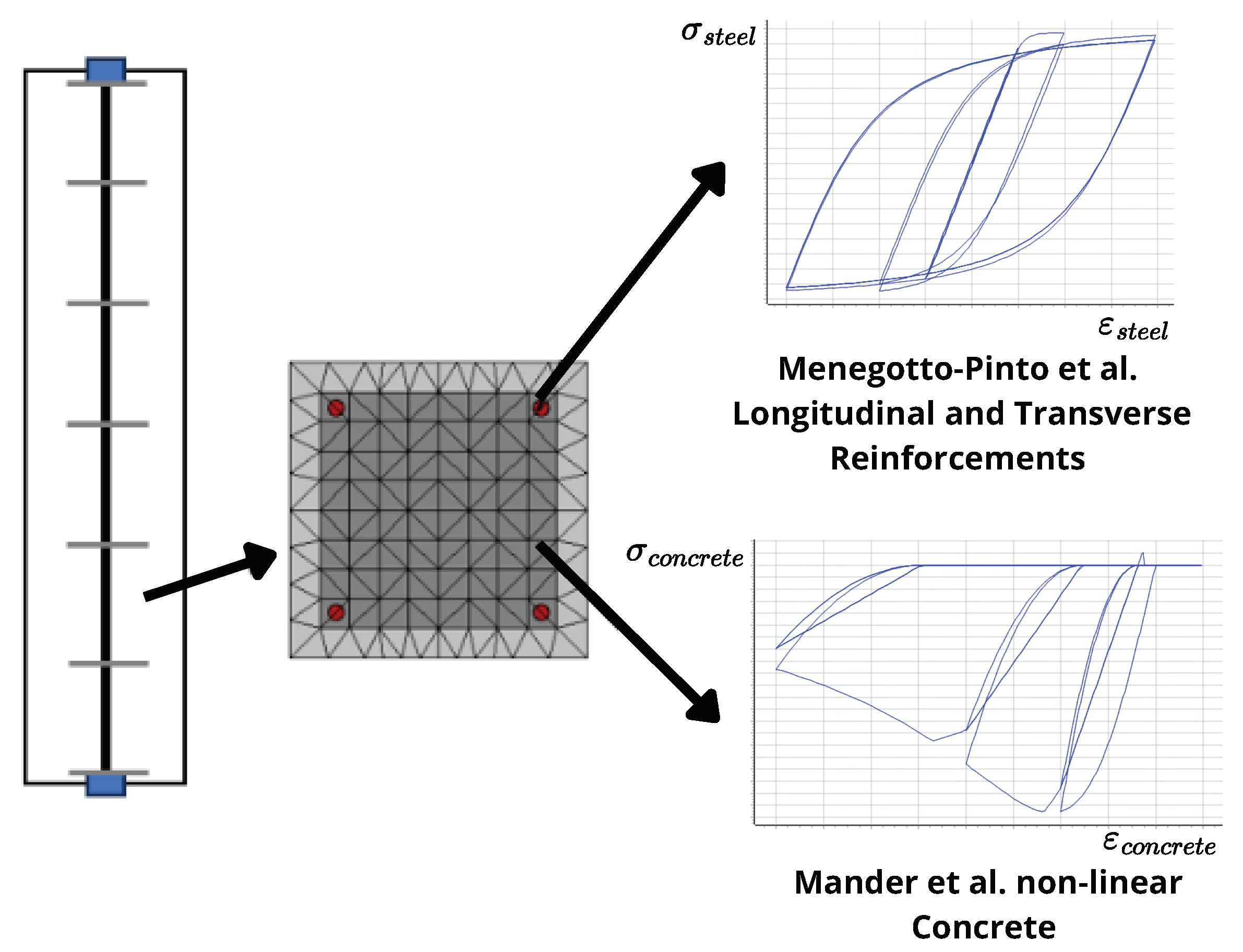
Figure 1.
Overview of the numerical simulation of RC elements [
17,
18].
Figure 1.
Overview of the numerical simulation of RC elements [
17,
18].
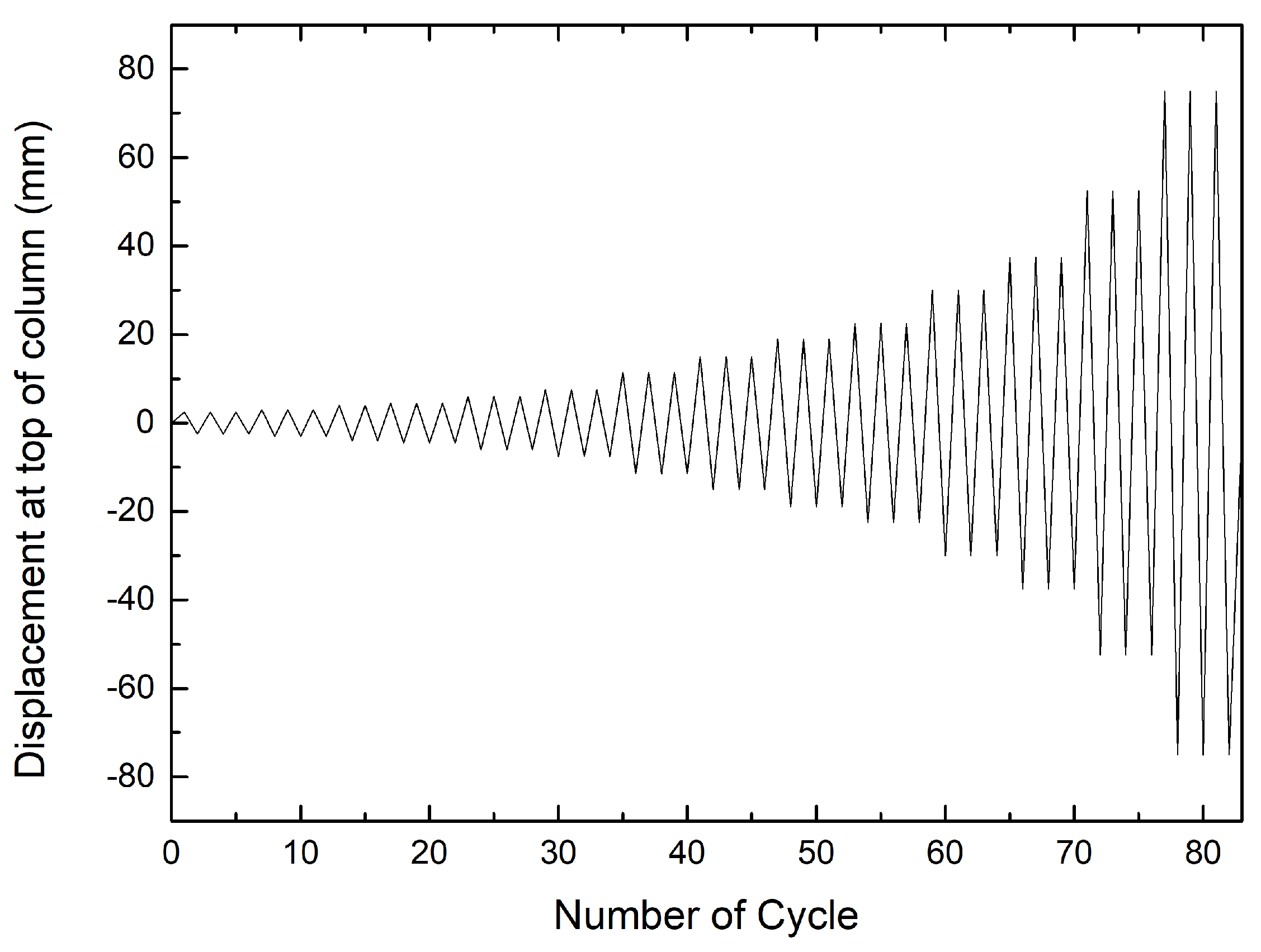
Figure 2.
Horizontal displacement history adopted in the tests performed by Meda et al. [
10].
Figure 2.
Horizontal displacement history adopted in the tests performed by Meda et al. [
10].
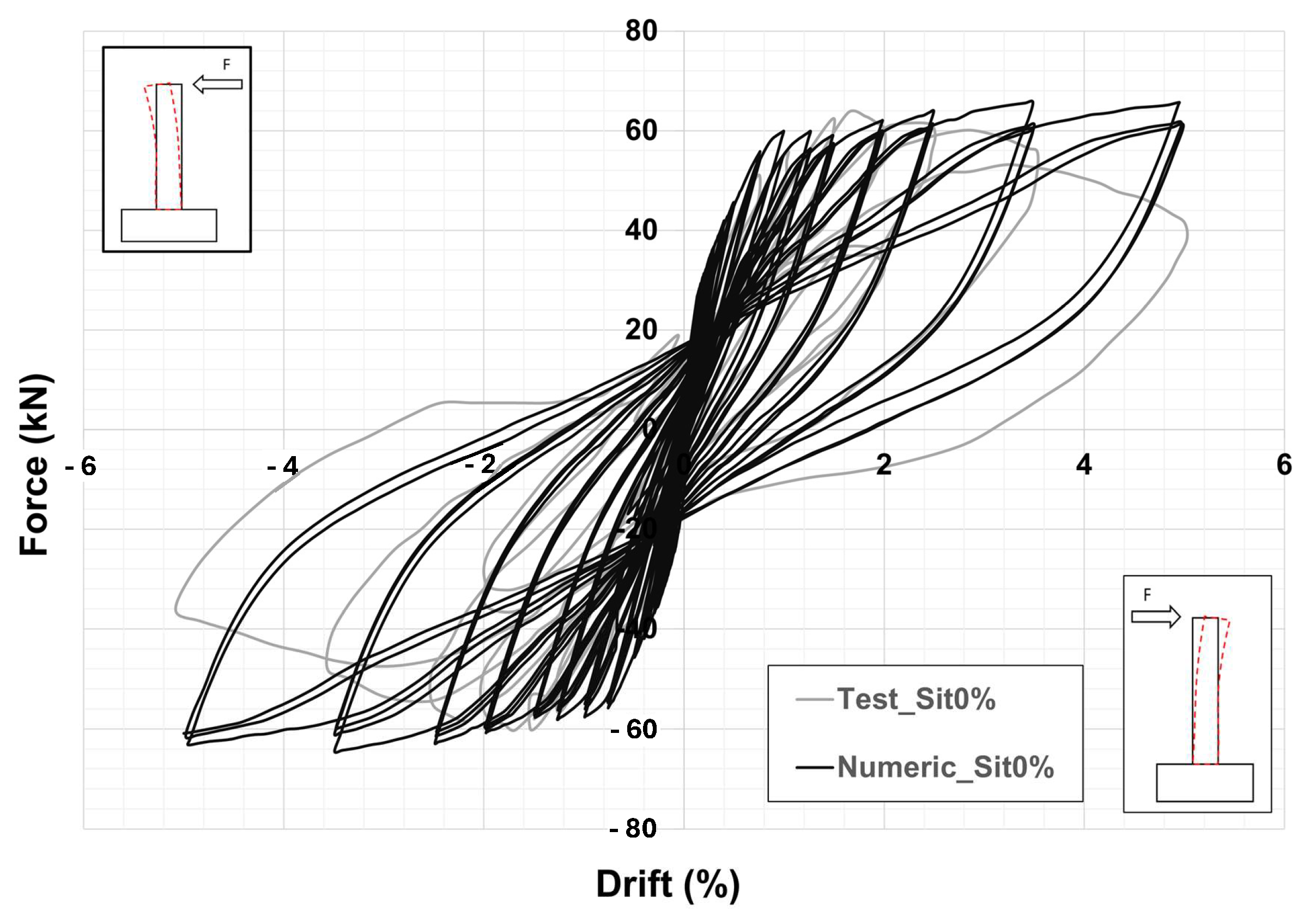
Figure 3.
Comparison of the force–drift response curves for the uncorroded column.
Figure 3.
Comparison of the force–drift response curves for the uncorroded column.
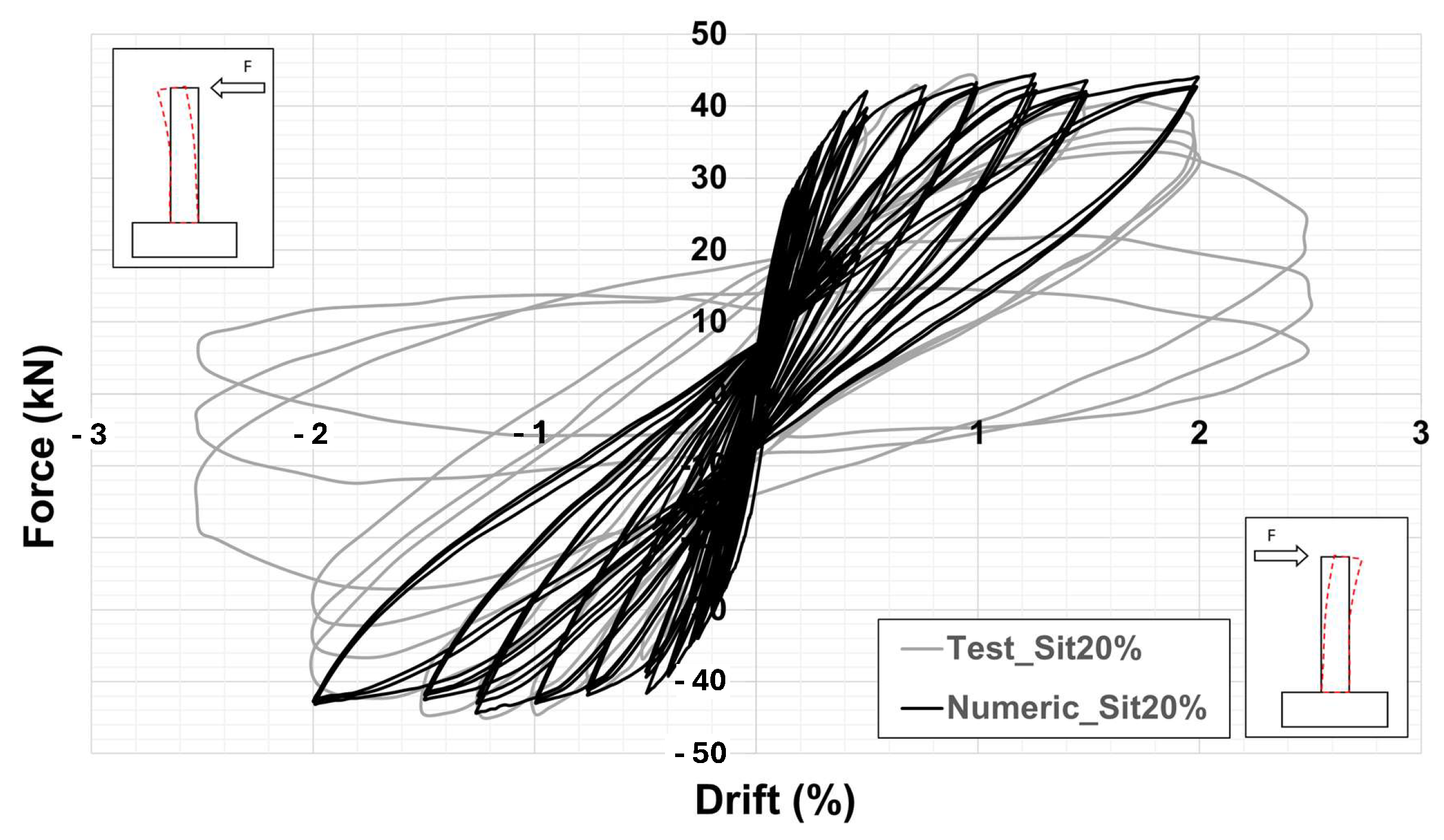
Figure 4.
Comparison of the force–drift response curves for the column with a corrosion rate of 20%.
Figure 4.
Comparison of the force–drift response curves for the column with a corrosion rate of 20%.
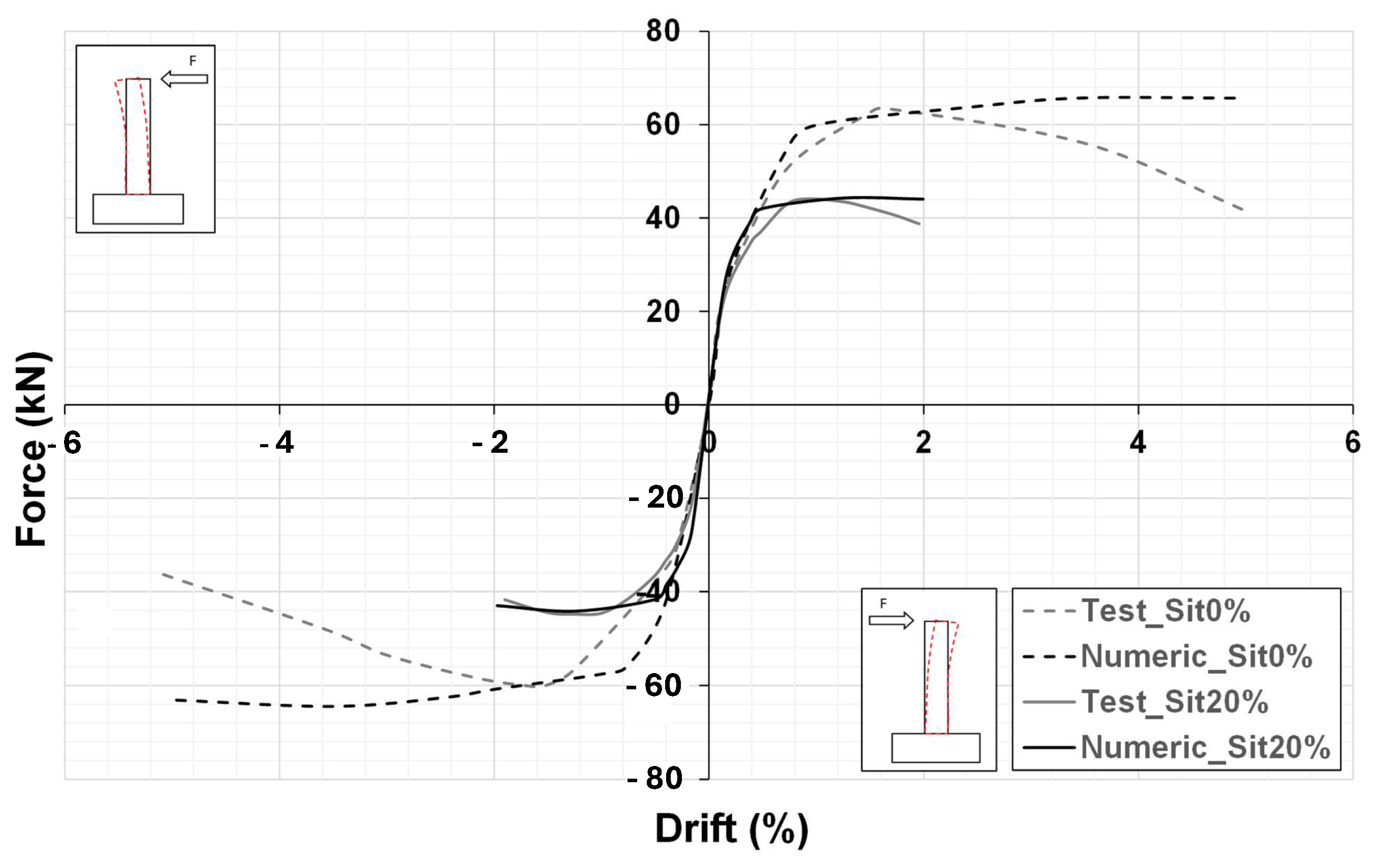
Figure 5.
Envelope curves of the experimental and numerical force–drift responses of the columns with and without corrosion.
Figure 5.
Envelope curves of the experimental and numerical force–drift responses of the columns with and without corrosion.
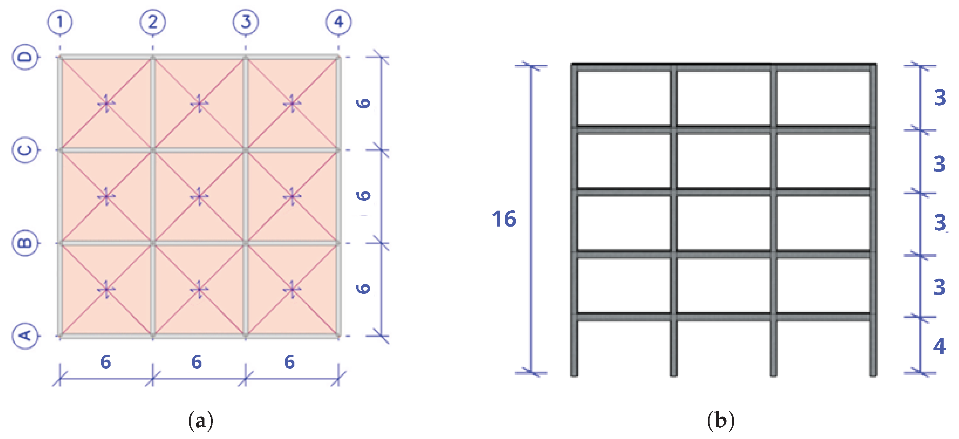
Figure 6.
Geometry: (
a) floor plan of the building (adapted from [
23]); (
b) front elevation (units in meters).
Figure 6.
Geometry: (
a) floor plan of the building (adapted from [
23]); (
b) front elevation (units in meters).
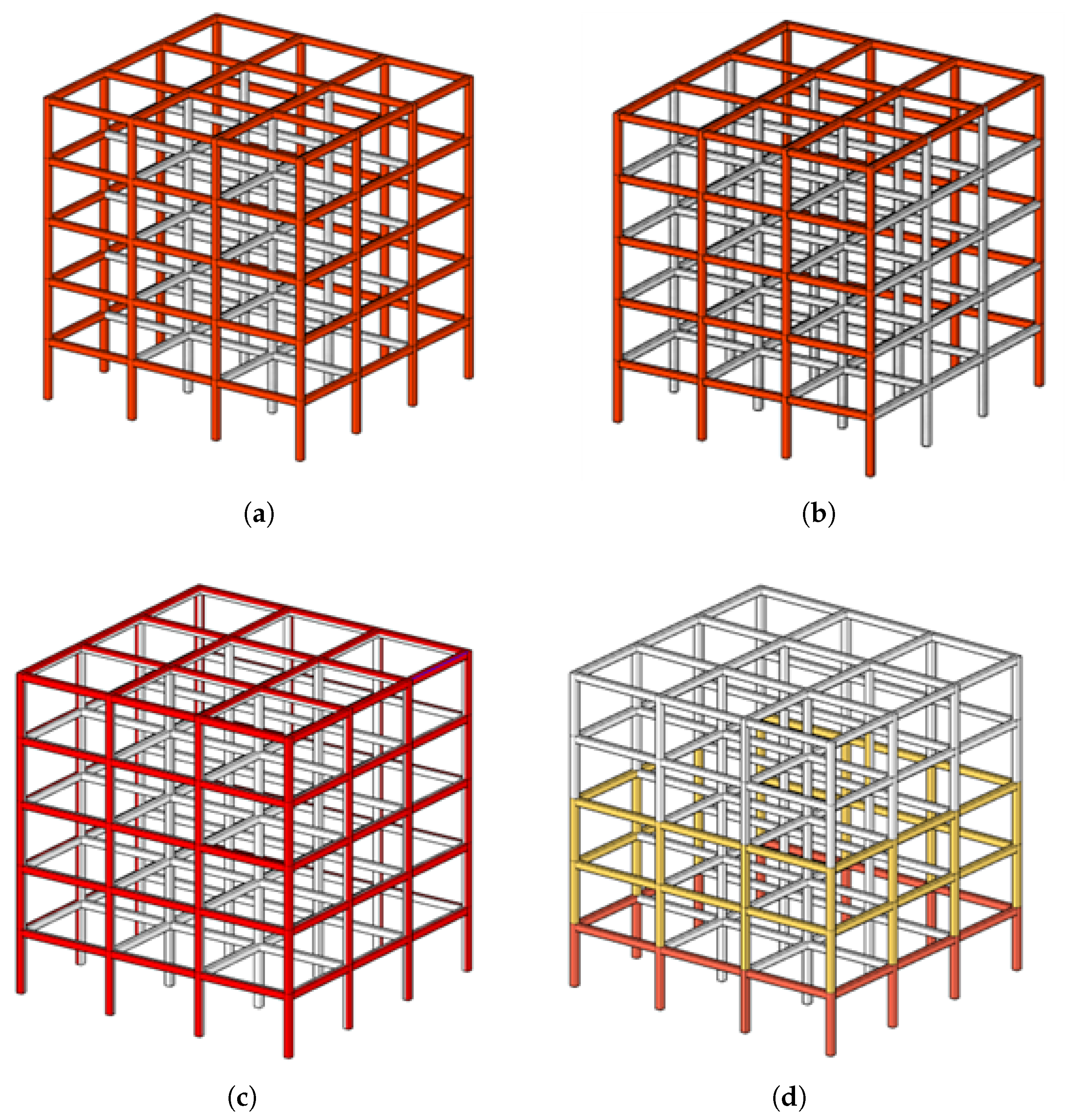
Figure 7.
Studied scenarios: (a) scenario 1; (b) scenario 2; (c) scenario 3; (d) scenario 4.
Figure 7.
Studied scenarios: (a) scenario 1; (b) scenario 2; (c) scenario 3; (d) scenario 4.
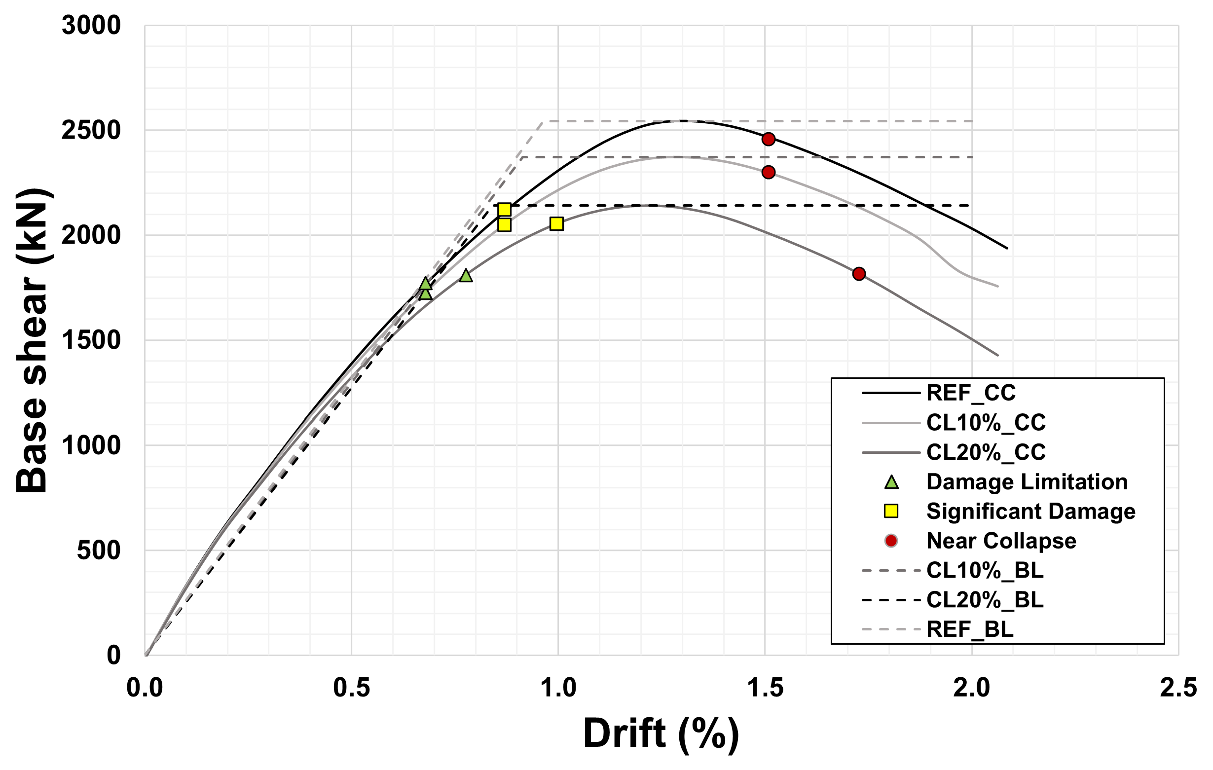
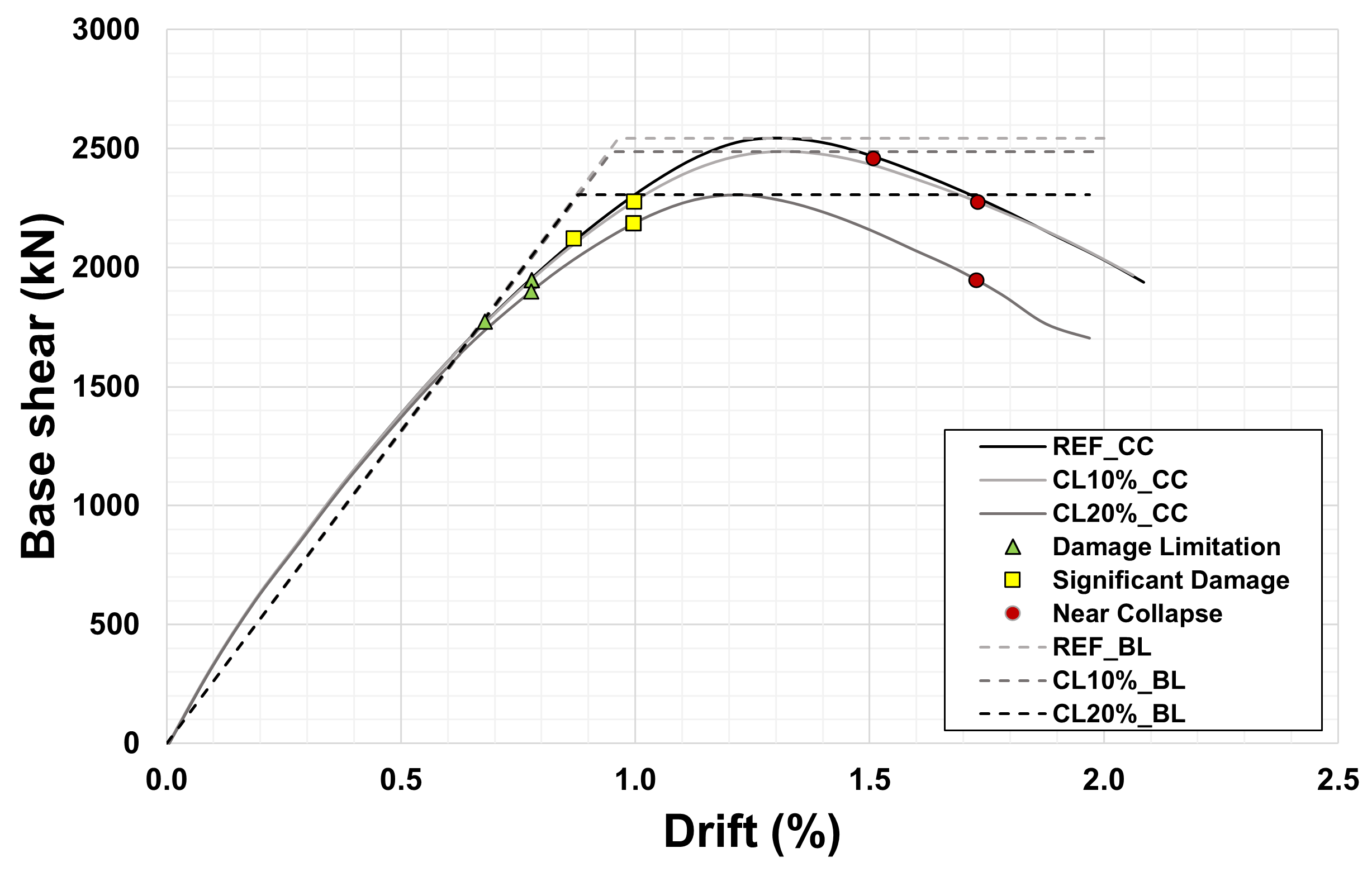
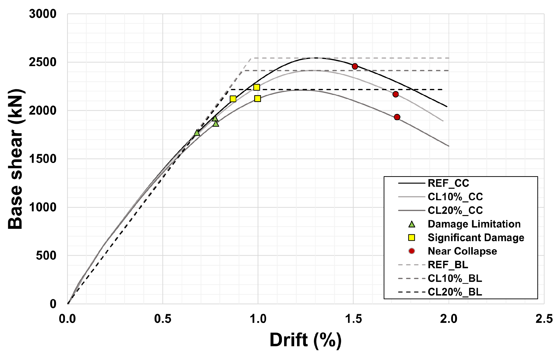
Figure 8.
Scenario 1: capacity curves (CC) and bilinear curves (BL) considering no corrosion and 10% and 20% corrosion levels (CLs).
Figure 8.
Scenario 1: capacity curves (CC) and bilinear curves (BL) considering no corrosion and 10% and 20% corrosion levels (CLs).
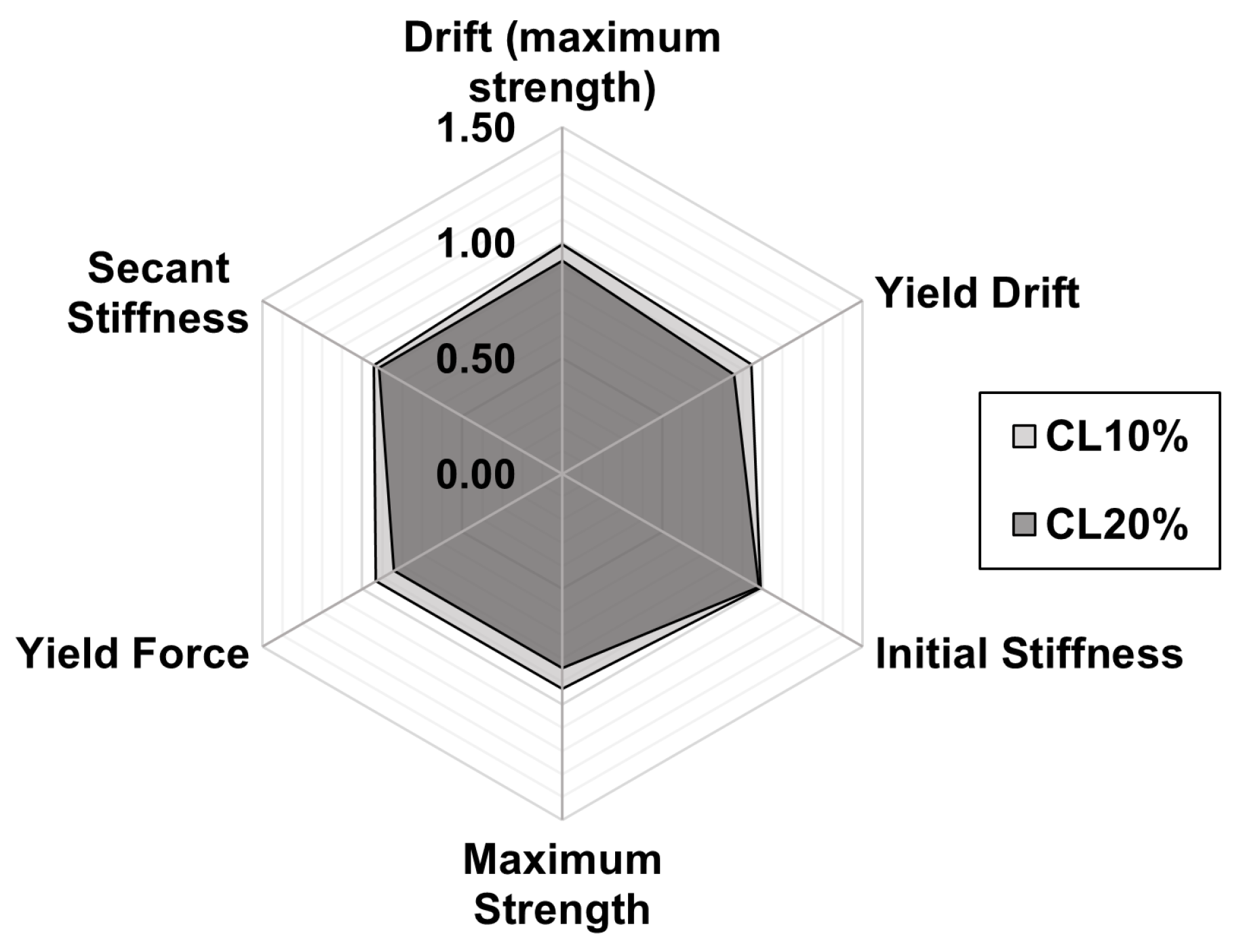
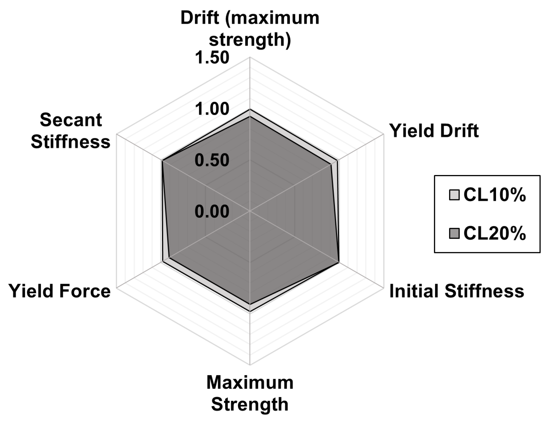
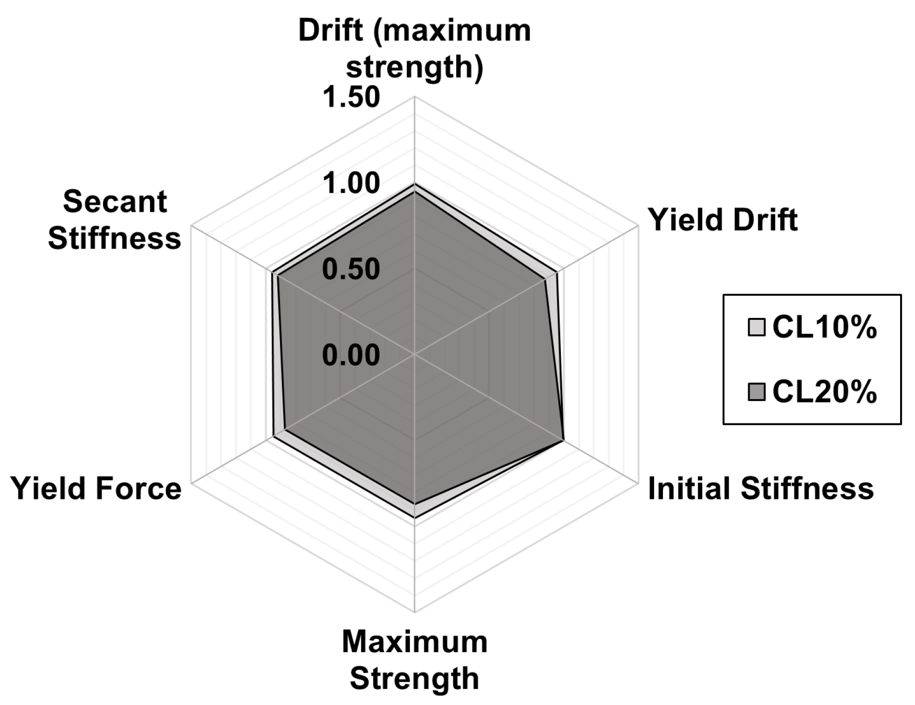
Figure 9.
Scenario 1: ratios of performance parameters with and without corrosion (for corrosion levels 10% and 20%).
Figure 9.
Scenario 1: ratios of performance parameters with and without corrosion (for corrosion levels 10% and 20%).
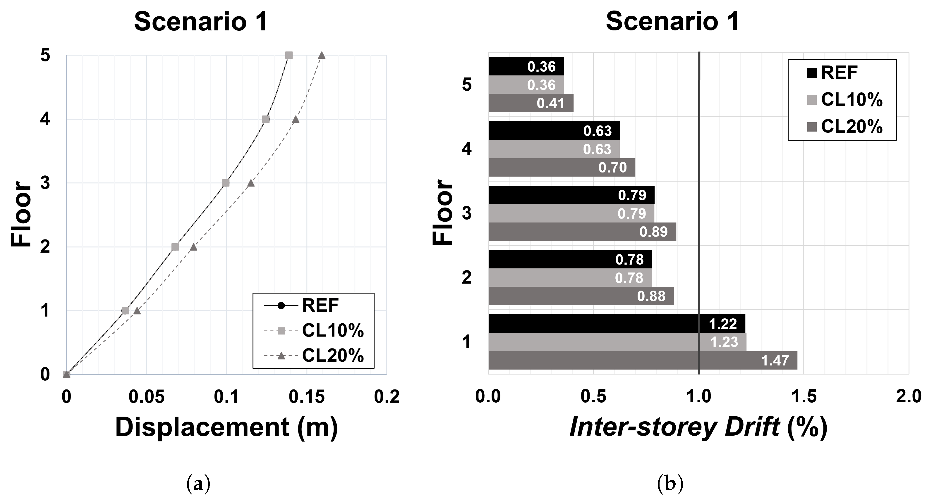
Figure 10.
Scenario 1: (a) displacement profile; and (b) inter-storey drift profile corresponding to the significant damage performance point.
Figure 10.
Scenario 1: (a) displacement profile; and (b) inter-storey drift profile corresponding to the significant damage performance point.
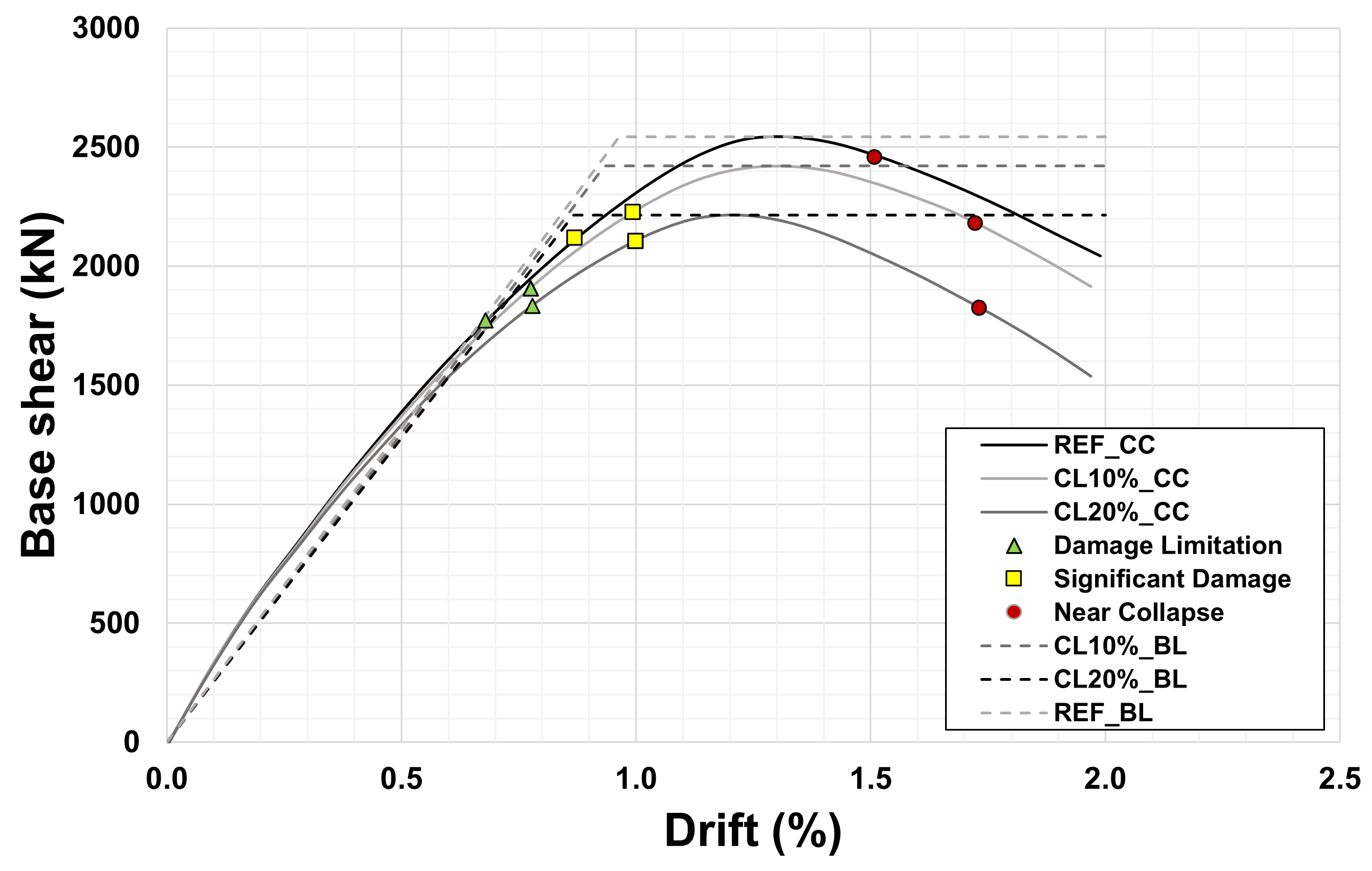
Figure 11.
Scenario 2.A: capacity curves (CCs) and bilinear curves (BLs) considering no corrosion and 10% and 20% corrosion levels (CLs).
Figure 11.
Scenario 2.A: capacity curves (CCs) and bilinear curves (BLs) considering no corrosion and 10% and 20% corrosion levels (CLs).
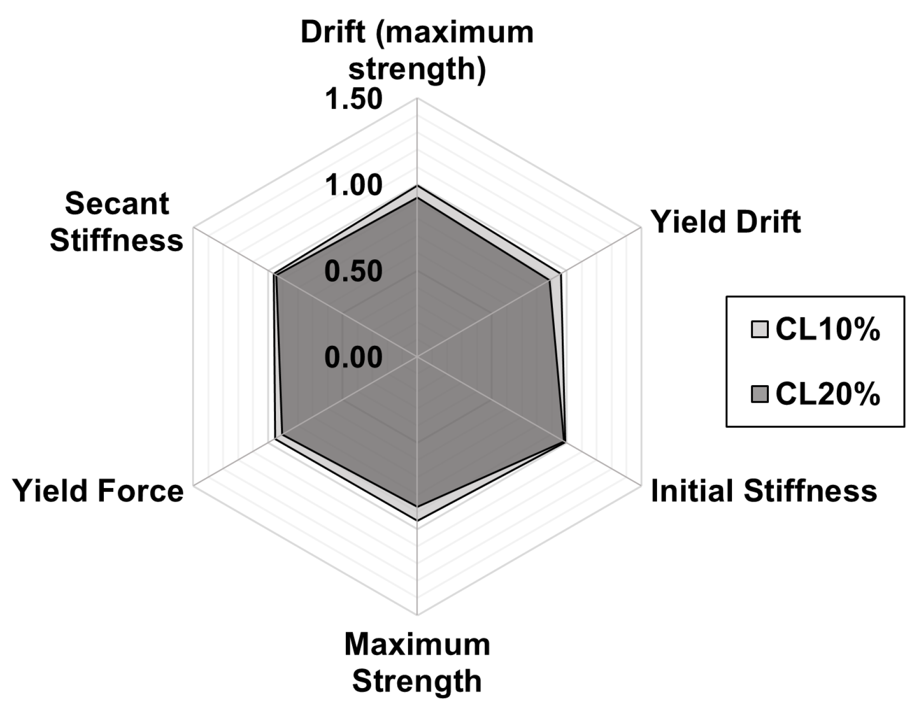
Figure 12.
Scenario 2.A: ratios of performance parameters with and without corrosion (for corrosion levels 10% and 20%).
Figure 12.
Scenario 2.A: ratios of performance parameters with and without corrosion (for corrosion levels 10% and 20%).
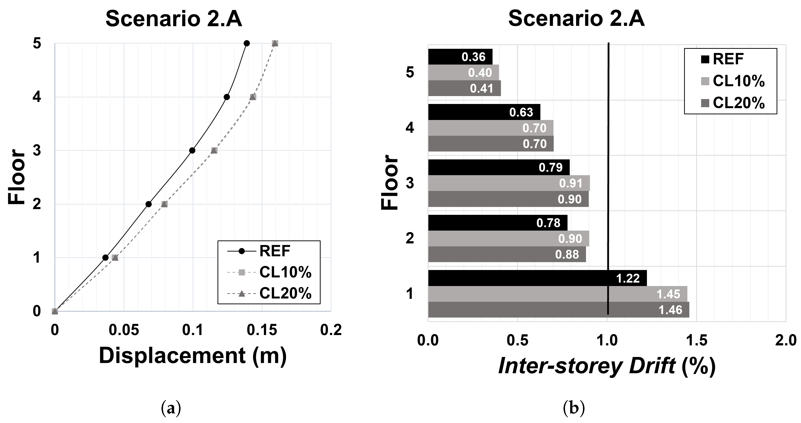
Figure 13.
Scenario 2.A: (a) displacement profile; and (b) inter-storey drift profile corresponding to the significant damage performance point.
Figure 13.
Scenario 2.A: (a) displacement profile; and (b) inter-storey drift profile corresponding to the significant damage performance point.
Figure 14.
Scenario 2.B: capacity curves (CCs) and bilinear curves (BLs) considering no corrosion and 10% and 20% corrosion levels (CLs).
Figure 14.
Scenario 2.B: capacity curves (CCs) and bilinear curves (BLs) considering no corrosion and 10% and 20% corrosion levels (CLs).
Figure 15.
Scenario 2.B: ratios of performance parameters with and without corrosion (for corrosion levels 10% and 20%).
Figure 15.
Scenario 2.B: ratios of performance parameters with and without corrosion (for corrosion levels 10% and 20%).
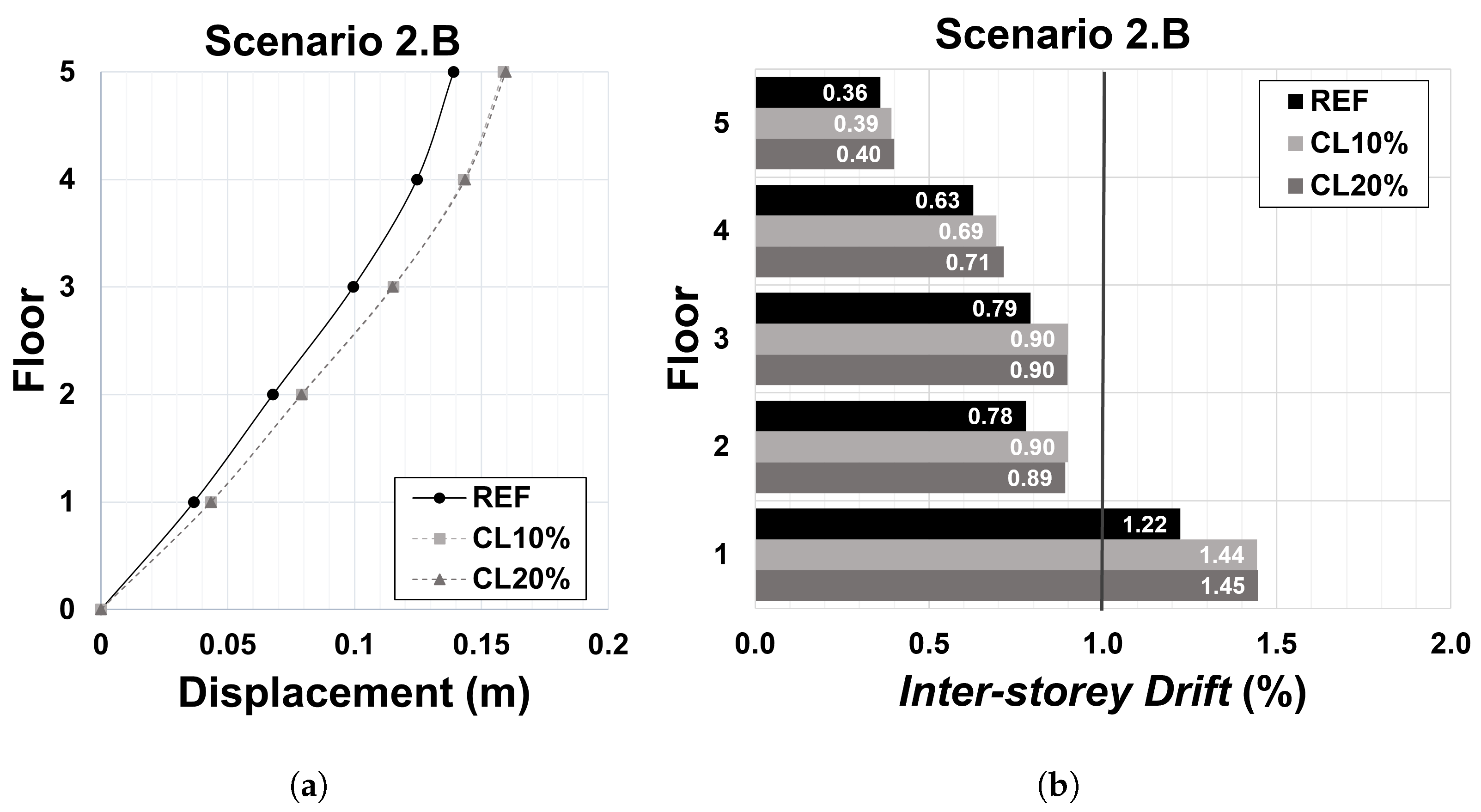
Figure 16.
Scenario 2.B: (a) displacement profile; and (b) inter-storey drift profile corresponding to the significant damage performance point.
Figure 16.
Scenario 2.B: (a) displacement profile; and (b) inter-storey drift profile corresponding to the significant damage performance point.
Figure 17.
Scenario 3: capacity curves (CCs) and bilinear curves (BLs) considering no corrosion and 10% and 20% corrosion levels (CLs).
Figure 17.
Scenario 3: capacity curves (CCs) and bilinear curves (BLs) considering no corrosion and 10% and 20% corrosion levels (CLs).
Figure 18.
Scenario 3: ratios of performance parameters with and without corrosion for corrosion levels 10% and 20%).
Figure 18.
Scenario 3: ratios of performance parameters with and without corrosion for corrosion levels 10% and 20%).
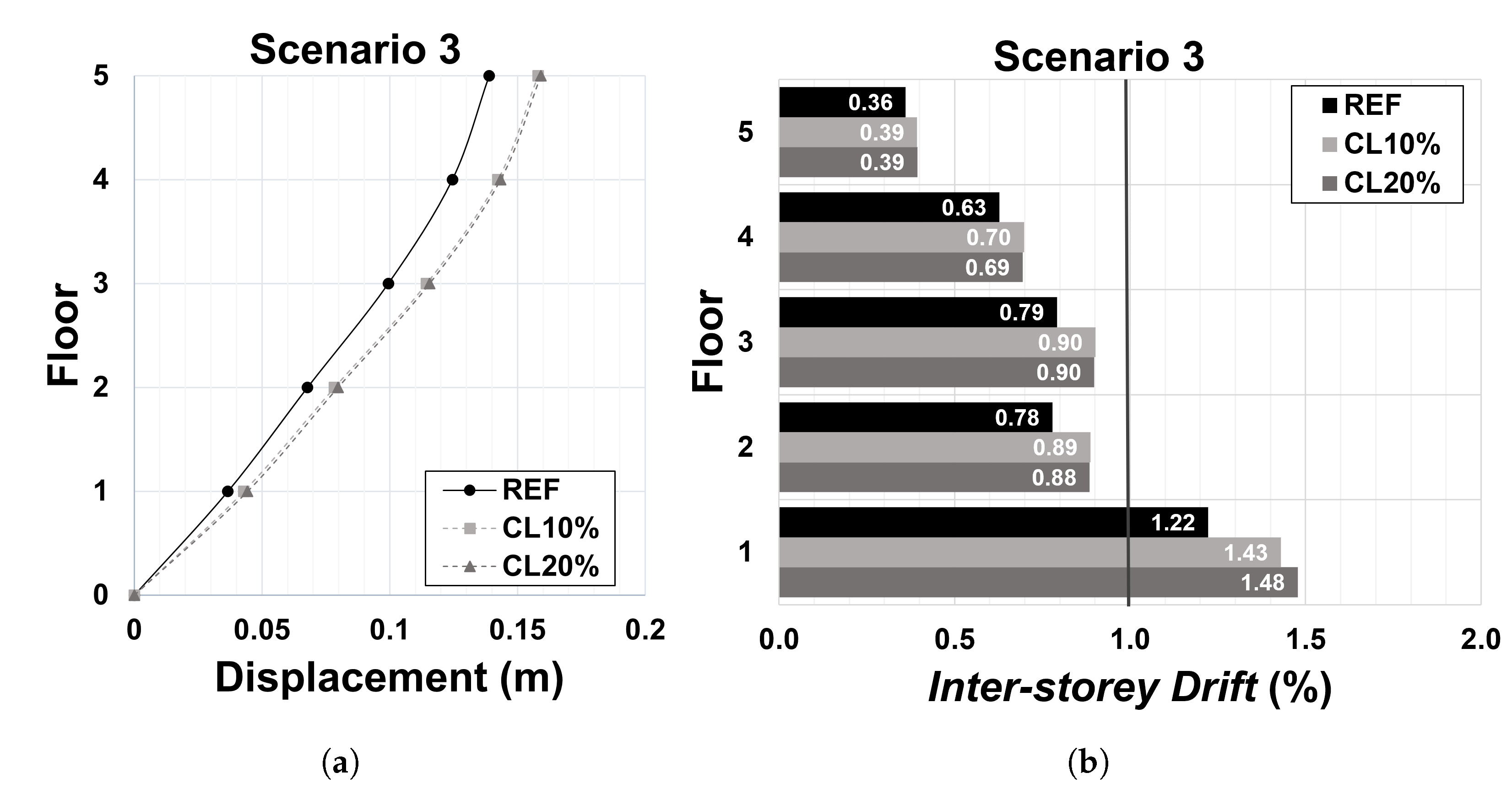
Figure 19.
Scenario 3: (a) displacement profile; and (b) inter-storey drift profile corresponding to the significant damage performance point.
Figure 19.
Scenario 3: (a) displacement profile; and (b) inter-storey drift profile corresponding to the significant damage performance point.
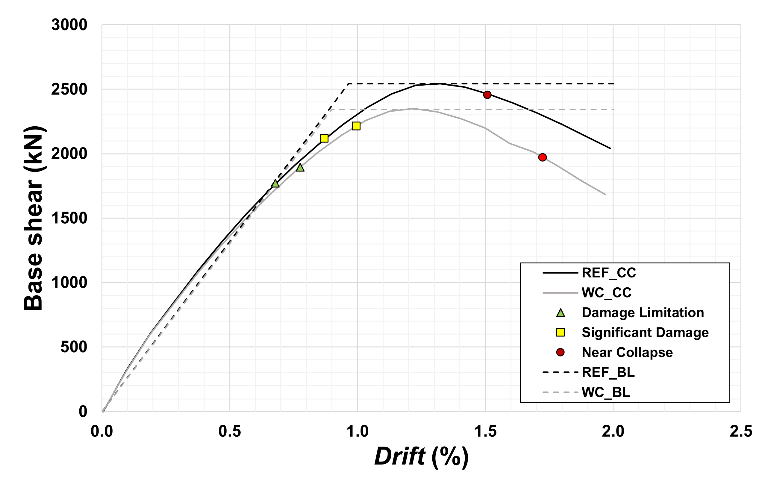
Figure 20.
Scenario 4: capacity curves (CCs) and bilinear curves (BLs) considering no corrosion and 10% and 20% corrosion levels (CLs).
Figure 20.
Scenario 4: capacity curves (CCs) and bilinear curves (BLs) considering no corrosion and 10% and 20% corrosion levels (CLs).
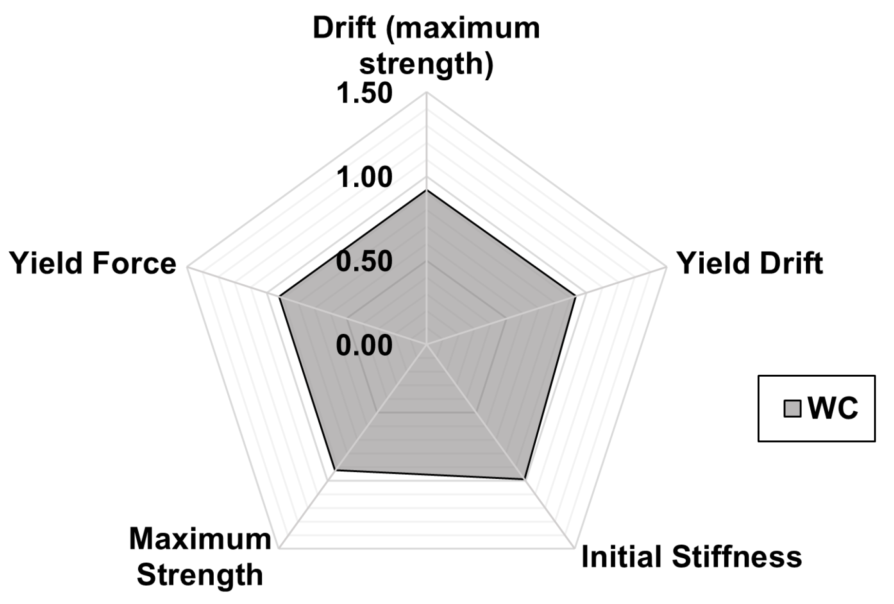
Figure 21.
Scenario 4: ratios of performance parameters with and without corrosion.
Figure 21.
Scenario 4: ratios of performance parameters with and without corrosion.
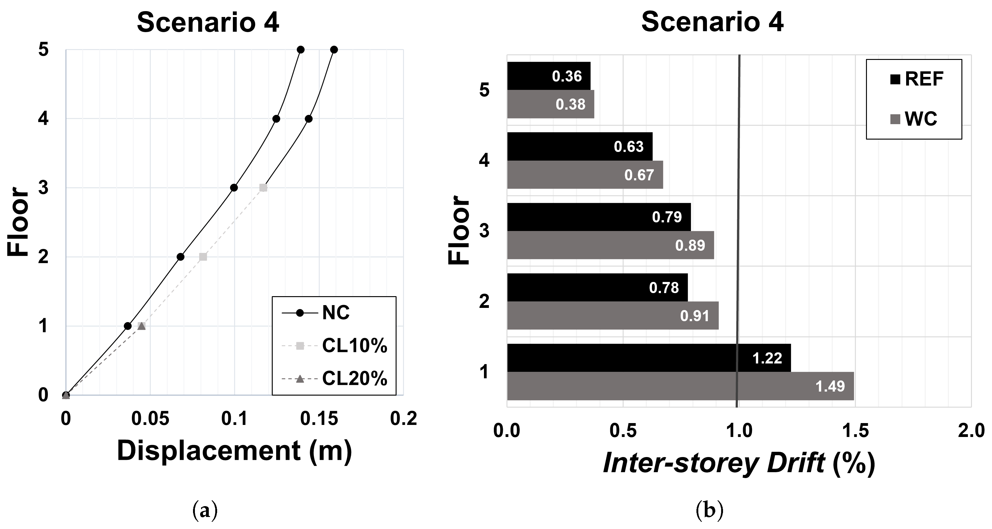
Figure 22.
Scenario 4: (a) displacement profile; and (b) inter-storey drift profile corresponding to the significant damage performance point.
Figure 22.
Scenario 4: (a) displacement profile; and (b) inter-storey drift profile corresponding to the significant damage performance point.
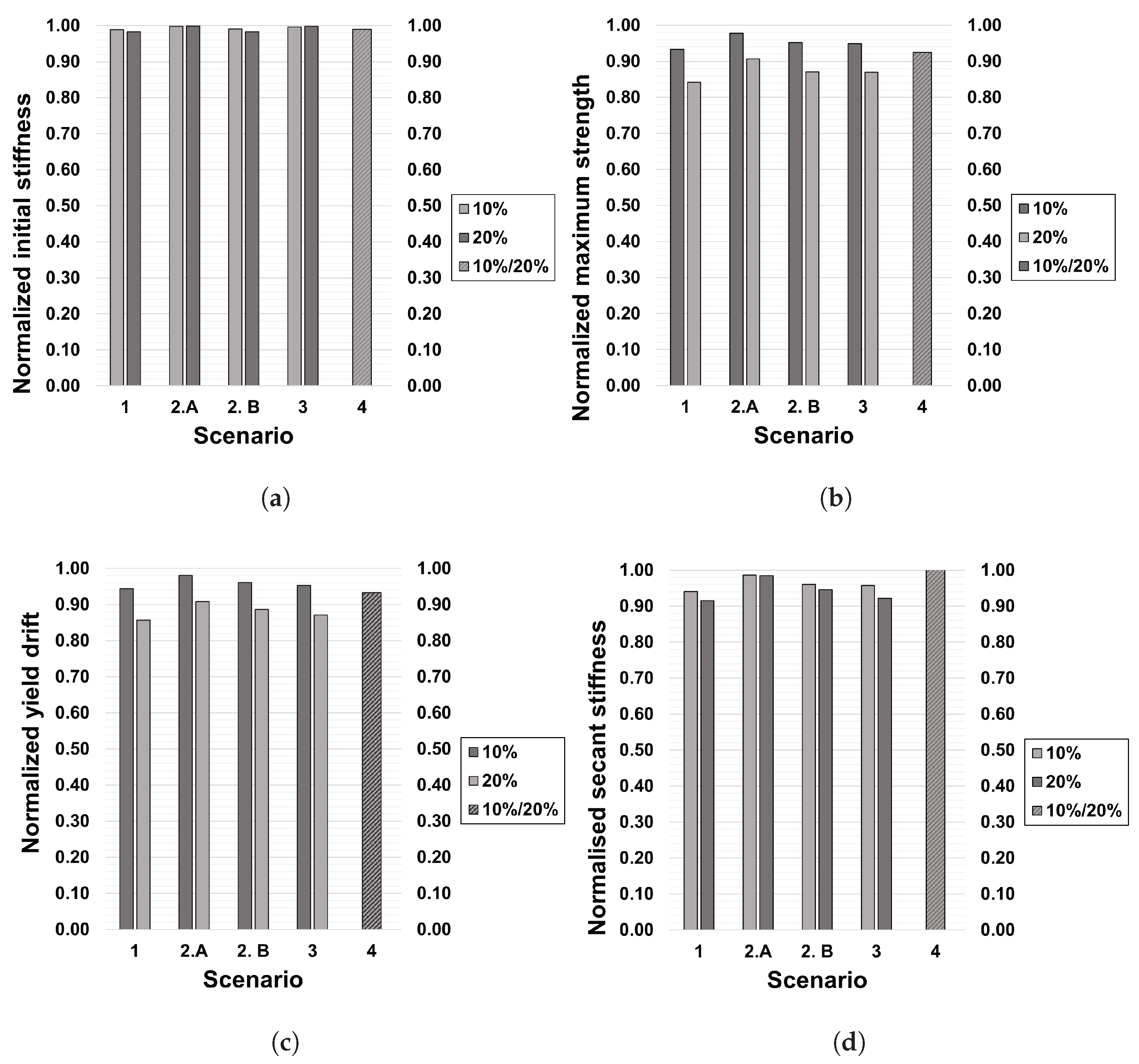
Figure 23.
Global comparison for each scenario: (a) normalized initial stiffness; (b) normalized maximum strength; (c) normalized yield drift; (d) normalized secant stiffness.
Figure 23.
Global comparison for each scenario: (a) normalized initial stiffness; (b) normalized maximum strength; (c) normalized yield drift; (d) normalized secant stiffness.
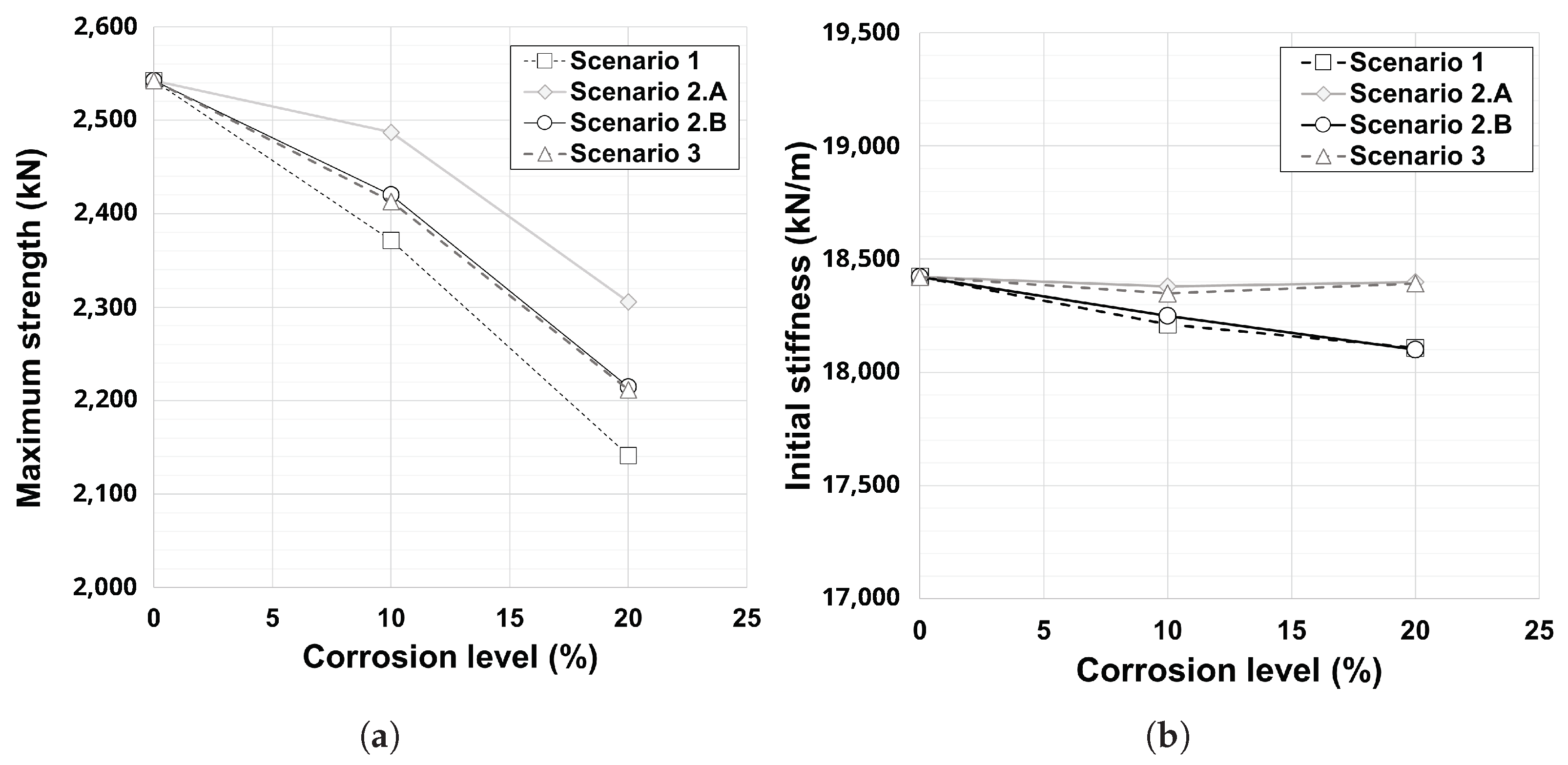
Figure 24.
(a) Variation of maximum strength with the increase in corrosion rate; (b) variation of initial stiffness with the increase in corrosion rate.
Figure 24.
(a) Variation of maximum strength with the increase in corrosion rate; (b) variation of initial stiffness with the increase in corrosion rate.
Table 1.
Mechanical properties (mean values) of steel and concrete according to Meda et al. [
10].
Table 1.
Mechanical properties (mean values) of steel and concrete according to Meda et al. [
10].
| Concrete | Steel |
|---|
| (MPa) | 20 | (MPa) | 520 |
| (MPa) | 2.2 | (%) | 13.72 |
| (GPa) | 30 | (GPa) | 210 |
Table 2.
Numerical parameters used to simulate the steel uniaxial material curve.
Table 2.
Numerical parameters used to simulate the steel uniaxial material curve.
| Corrosion Level | 0% | 20% | Ratio |
|---|
| (GPa) | 210 | 210 | 1.00 |
| (MPa) | 520 | 312 | 0.60 |
| 0.015 | 0.015 | 1.00 |
| 20 | 18.9 | 0.95 |
| 19.6 | 18.6 | 0.95 |
| 0.15 | 0.15 | 1.00 |
| P | 0.6 | 0.6 | 1.00 |
| r (%) | 2.5 | 5.00 | 2.00 |
| 0.1372 | 0.0410 | 0.30 |
| (kN/m3) | 78.00 | 78.00 | 1.00 |
Table 3.
Numerical parameters used to simulate the concrete uniaxial material curve.
Table 3.
Numerical parameters used to simulate the concrete uniaxial material curve.
| Concrete |
|---|
| (MPa) | (MPa) | (GPa) | | (kN/m3) |
| 20 | 2.2 | 30 | 0.02 | 24 |
Table 4.
Key parameters of experimental and numerical response.
Table 4.
Key parameters of experimental and numerical response.
| Corrosion Level | Cycles | Model | Initial Stiffness (kN/m) | Maximum Strength (kN) | Drift (Maximum Strength) (%) |
|---|
| 0% | Positive | Experimental | 9068 | 63.53 | 1.63 |
| Positive | Numerical | 10,215 | 65.74 | 3.49 |
| Negative | Experimental | 6900 | 60.11 | 1.53 |
| Negative | Numerical | 7004 | 64.48 | 3.49 |
| 20% | Positive | Experimental | 10,857 | 44.21 | 1.21 |
| Positive | Numerical | 11,891 | 44.48 | 1.26 |
| Negative | Experimental | 7022 | 44.81 | 1.24 |
| Negative | Numerical | 7426 | 44.36 | 1.27 |
Table 5.
Ratios of key parameters.
Table 5.
Ratios of key parameters.
| Corrosion Level | Cycles | Initial Stiffness (kN/m) | Maximum Strength (kN) | Drift (Maximum Strength) (%) |
|---|
| 0% | Positive | 1.13 | 1.03 | 2.13 |
| Negative | 1.02 | 1.07 | 2.28 |
| 20% | Positive | 1.10 | 1.01 | 1.04 |
| Negative | 1.06 | 0.99 | 1.02 |
Table 6.
Vertical loads considered for the case study.
Table 6.
Vertical loads considered for the case study.
| Load Type | Floor | Load | Value |
|---|
| Structure self-weight (Gk,1) | All floors | Primary seismic members (columns and beams)
Slabs: solid RC 15 cm thick | |
Other permanent
loads (Gk,2) | 1st to | External walls and partitions with (per unit of wall length) | |
| | Finishings | |
| (n)th (roof) | Finishings | |
Live
loads (Qk) | 1st to | Building for use as civil dwellings, falling into usage category A | |
| (n)th (roof) | Roof category H—Roofs not accessible except for normal maintenance and repair | |
Table 7.
Scenario 1: extracted response parameters for each corrosion level.
Table 7.
Scenario 1: extracted response parameters for each corrosion level.
| Response Parameters | Ref | CL 10% | CL 20% |
|---|
| Initial Stiffness (kN/m) | 18,422 | 18,211 | 18,108 |
| Maximum Strength (kN) | 2542 | 2371 | 2141 |
| Drift (Maximum Strength) (%) | 1.32 | 1.31 | 1.22 |
| Secant Stiffness (kN/m) | 12,003 | 11,293 | 10,981 |
| Yield Force (kN) | 1017 | 949 | 857 |
| Yield Drift (%) | 0.35 | 0.33 | 0.30 |
Table 8.
Scenario 1: Corresponding base shear and drift for each of the performance points.
Table 8.
Scenario 1: Corresponding base shear and drift for each of the performance points.
| Corrosion Level | 0% | 10% | 20% |
|---|
| Damage Limitation | Base shear (kN) | 1773 | 1725 | 1810 |
| Drift (%) | 0.68 | 0.68 | 0.78 |
| Significant Damage | Base shear (kN) | 2119 | 2048 | 2052 |
| Drift (%) | 0.87 | 0.87 | 1.00 |
| Near Collapse | Base shear (kN) | 2456 | 2297 | 1813 |
| Drift (%) | 1.51 | 1.51 | 1.73 |
Table 9.
Scenario 2.A: extracted response parameters for each corrosion level.
Table 9.
Scenario 2.A: extracted response parameters for each corrosion level.
| Response Parameters | Ref | CL 10% | CL 20% |
|---|
| Initial Stiffness (kN/m) | 18,422 | 18,380 | 18,399 |
| Maximum Strength (kN) | 2542 | 2487 | 2306 |
| Drift (Maximum Strength) (%) | 1.32 | 1.31 | 1.22 |
| Secant Stiffness (kN/m) | 12,003 | 11,843 | 11,824 |
| Yield Force (kN) | 1017 | 995 | 922 |
| Yield Drift (%) | 0.35 | 0.34 | 0.31 |
Table 10.
Scenario 2.A: corresponding base shear and drift of performance points.
Table 10.
Scenario 2.A: corresponding base shear and drift of performance points.
| Corrosion Level | 0% | 10% | 20% |
|---|
| Damage Limitation | Base shear (kN) | 1773 | 1946 | 1899 |
| Drift (%) | 0.68 | 0.78 | 0.78 |
| Significant Damage | Base shear (kN) | 2119 | 2276 | 2184 |
| Drift (%) | 0.87 | 1.00 | 1.00 |
| Near Collapse | Base shear (kN) | 2456 | 2273 | 1943 |
| Drift (%) | 1.51 | 1.73 | 1.73 |
Table 11.
Scenario 2.B: extracted response parameters for each corrosion level.
Table 11.
Scenario 2.B: extracted response parameters for each corrosion level.
| Response Parameters | Ref | CL 10% | CL 20% |
|---|
| Initial Stiffness (kN/m) | 18,422 | 18,249 | 18,108 |
| Maximum Strength (kN) | 2542 | 2420 | 2215 |
| Drift (Maximum Strength) (%) | 1.32 | 1.31 | 1.22 |
| Secant Stiffness (kN/m) | 12.003 | 11,524 | 11,357 |
| Yield Force (kN) | 1017 | 968 | 922 |
| Yield Drift (%) | 0.35 | 0.33 | 0.31 |
Table 12.
Scenario 2.B: corresponding base shear and drift of performance points.
Table 12.
Scenario 2.B: corresponding base shear and drift of performance points.
| Corrosion Level | 0% | 10% | 20% |
|---|
| Damage Limitation | Base shear (kN) | 1773 | 1907 | 1833 |
| Drift (%) | 0.68 | 0.78 | 0.78 |
| Significant Damage | Base shear (kN) | 2119 | 2226 | 2104 |
| Drift (%) | 0.87 | 0.99 | 1.00 |
| Near Collapse | Base shear (kN) | 2456 | 2180 | 1824 |
| Drift (%) | 1.51 | 1.72 | 1.73 |
Table 13.
Scenario 3: extracted response parameters for each corrosion level.
Table 13.
Scenario 3: extracted response parameters for each corrosion level.
| Response Parameters | Ref | CL 10% | CL 20% |
|---|
| Initial Stiffness (kN/m) | 18,422 | 18,348 | 18,392 |
| Maximum Strength (kN) | 2542 | 2413 | 2211 |
| Drift (Maximum Strength) (%) | 1.32 | 1.31 | 1.25 |
| Secant Stiffness (kN/m) | 12,003 | 11,491 | 11,057 |
| Yield Force (kN) | 1017 | 965 | 885 |
| Yield Drift (%) | 0.35 | 0.33 | 0.30 |
Table 14.
Scenario 3: corresponding base shear and drift of performance points.
Table 14.
Scenario 3: corresponding base shear and drift of performance points.
| Corrosion Level | 0% | 10% | 20% |
|---|
| Damage Limitation | Base shear (kN) | 1773 | 1922 | 1866 |
| Drift (%) | 0.68 | 0.77 | 0.78 |
| Significant Damage | Base shear (kN) | 2119 | 2239 | 2121 |
| Drift (%) | 0.87 | 0.99 | 1.00 |
| Near Collapse | Base shear (kN) | 2456 | 2167 | 1930 |
| Drift (%) | 1.51 | 1.72 | 1.73 |
Table 15.
Scenario 4: extracted response parameters for each corrosion level.
Table 15.
Scenario 4: extracted response parameters for each corrosion level.
| Response Parameters | Ref | WC |
|---|
| Initial Stiffness (kN/m) | 18,422 | 18,243 |
| Maximum Strength (kN) | 2542 | 2349 |
| Drift (Maximum Strength) (%) | 1.32 | 1.22 |
| Secant Stiffness (kN/m) | 12,003 | 12,048 |
| Yield Force (kN) | 1017 | 940 |
| Yield Drift (%) | 0.35 | 0.32 |
Table 16.
Scenario 4: corresponding base shear and drift of performance points.
Table 16.
Scenario 4: corresponding base shear and drift of performance points.
| Corrosion Level | Ref | WC |
|---|
| Damage Limitation | Base shear (kN) | 1773 | 1896 |
| Drift (%) | 0.68 | 0.78 |
| Significant Damage | Base shear (kN) | 2119 | 2213 |
| Drift (%) | 0.87 | 1.00 |
| Near Collapse | Base shear (kN) | 2456 | 1969 |
| Drift (%) | 1.51 | 1.73 |


